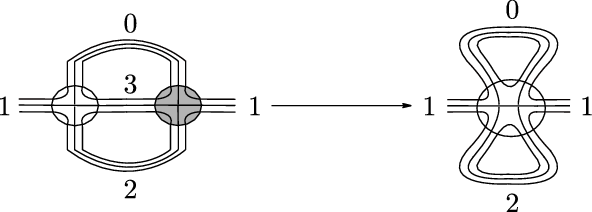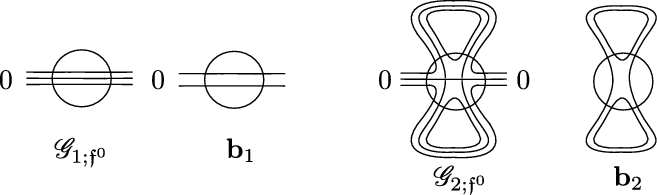



1. Background and main results
The Tutte polynomial is a universal polynomial invariant defined on abstract graphs. This invariant obeys a particular recursion relation for the contraction and deletion of the edges of a graph, see for instance [Reference Tutte29]. The Bollobás–Riordan (BR) polynomial, see [Reference Bollobás and Riordan9, Reference Bollobás and Riordan10], defines a genuine extension of the Tutte polynomial to ribbon graphs or neighbourhoods of graphs embedded in surfaces. Before, in the context of quantum groups, Reshetikhin and Turaev showed in [Reference Reshetikhin and Turaev26] the existence of a generalized Jones polynomial on graphs embedded in surfaces.
In this work, we investigate families of combinatorial objects generalizing abstract and ribbon graphs to which both the Tutte and BR polynomial invariants may be extended. These generalized graphs were identified as Feynman graphs of matrix [Reference Di Francesco, Ginsparg and Zinn-Justin15] and tensor models [Reference Ambjorn, Durhuus and Jonsson1]. Such models in physics aim at defining a quantum spacetime, and their graphs represent discrete geometries. The study of coloured tensor graphs, i.e. the Feynman graphs of coloured tensor models introduced in [Reference Gurau17] (see also [Reference Ben Geloun, Magnen and Rivasseau6, Reference Gurau20, Reference Gurau and Ryan21]), has acknowledged a growing interest after the recent discovery, by Gurau in [Reference Gurau19], of the main organizing tool of their partition function. The story of coloured tensor graphs has also been successful from the point of view of combinatorics and graph theory because of their tractable properties. For instance, well-known combinatorial notions defined on graphs such as polynomial invariants and Hopf-algebras have been extended to tensor graphs in [Reference Avohou, Rivasseau and Tanasa5, Reference Gurau20, Reference Raasakka and Tanasa27, Reference Tanasa28].
There are two main worksFootnote 1 addressing a generalization of the BR polynomial to a family of generalized graphs similar to that presented here: the works by Gurau in [Reference Gurau20] and by Tanasa in [Reference Tanasa28]. For tensor graphs, the vertex is stranded, and the usual way of contracting an edge immediately leads to a different vertex. As a consequence, the simplest prescriptions of contracting and deleting edges are not well defined without further considerations. Indeed, the two aforementioned works undertake the definition of the contraction and deletion of edges in an unusual manner.
There are several layers of difficulties while defining the type of graphs that ought to be considered. One should also distinguish the type of topological polynomial defined for the family of graphs, and the type of recursion relations that the invariant polynomial needs to satisfy. Our method is radically different from that of Tanasa, since we use the Gurau coloured prescription to keep under control the type of generated graphs. Moreover, and in contrast with the work by Gurau, we propose to enlarge the family of coloured tensor graphs to what is called weakly coloured (w-coloured) stranded graphs, for which contraction, and a similar notion of deletion make sense. These w-coloured stranded graphs are precisely the result of edge contractions of coloured tensor graphs. This class of graphs is closed under contraction. From this stability, we can define, for w-coloured graphs, a polynomial which is invariant under a linear recursion relation. We must mention that there might be room for improvement for the present definition of w-coloured stranded graphs. Although this is not needed in our analysis, there could be an equivalent description in terms of its basic constituents. Such a study is left for the future.
Our main result appears in Theorem 4.32 of Section 4. This statement determines the contraction and cut (an operation replacing the deletion) recursion relation with respect to an edge, fulfilled by a new polynomial given in Definition 4.27. The class of graphs on which the polynomial is defined has several components. Some of these components turn out to be well defined for abstract and ribbon graphs, and therefore, they are introduced step by step in the sequel.
A first component is captured by the notion of half-edge which can be introduced at the abstract graph level. Half-edges are of crucial importance in Physics, see [Reference Krajewski, Rivasseau and Vignes-Tourneret23, Reference Krajewski, Rivasseau, Tanasa and Wang24], for instance. The analysis of half-edged graphs (HEGs) is the purpose of Section 2. The Tutte polynomial for HEGs satisfies linear recursion identities similar to those of the Tutte polynomial for abstract graphs (see Definition 2.9), and so it turns out to be an evaluation of it.
A second key notion we need is that of open and closed faces of a ribbon graph with ribbon half-edges. The consequences that open and closed faces in a ribbon graph have on the related BR polynomial, are addressed in Section 3. Another important result of this work is set in Theorem 3.11, which establishes a new recursion relation obeyed by the BR polynomial for ribbon graphs with ribbon half-edges. Then follow the concluding remarks in Section 5.
Finally, a closing appendix provides explicit examples of the polynomial obtained for some w-coloured graphs.
2. HEGs and the Tutte polynomial
We start by setting up our graph theoretic notation.
2.1. Basic definitions and notation
We use
 $G(\mathcal{V},\mathcal{E})$
, or at times just G, to denote a graph (which allows loops and multiple edges) with vertex set
 $\mathcal{V}$
and edge set
 $\mathcal{E}$
.
We denote a spanning subgraph
 $A(\mathcal{V},\mathcal{E}_A)$
of a graph
 $G(\mathcal{V},\mathcal{E})$
by
 $A \subset G$
. Consider two disjoint graphs
 $G_1(\mathcal{V}_1,\mathcal{E}_1)$
and
 $G_2(\mathcal{V}_2,\mathcal{E}_2)$
. The disjoint union of the graphs
 $G_1$
and
 $G_2$
is denoted by
 $G_1 \sqcup G_2$
. The one-point join graph
 $G_1 \cdot _{v_1,v_2} G_2$
simply merges the two graphs at the vertices
 $v_1 \in \mathcal{V}_1$
and
 $v_2 \in \mathcal{V}_2$
, by removing
 $v_1$
and
 $v_2$
, and inserting a new vertex v which has all edges incident to
 $v_1$
and to
 $v_2$
.
Using the notation of [Reference Bollobás8], we have the following definition.
Definition 2.1 (Tutte polynomial). Let
 $G(\mathcal{V},\mathcal{E})$
be a graph, then the Tutte polynomial
 $T_{G}$
of G is defined as
 \begin{equation} T_{G}(x,y)=\sum_{A\subset G}(x-1)^{r(G)-r (A)}(y-1)^{n(A)},\end{equation}
where k(A) is the number of connected components of the spanning subgraph A,
 $r(A)=|\mathcal{V}|-k(A)$
its rank, and
 $n(A)=|\mathcal{E}_A|+k(A)-|\mathcal{V}|$
is its nullity or cyclomatic number.
There is an equivalent definition of this polynomial (in notation of [Reference Bollobás8]):
Definition 2.2 (Tutte polynomial 2). The Tutte polynomial
 $T_{G}$
of G is defined as:
a. If G has no edges, then
 $T_{G}(x,y)=1.$
Otherwise, for any edge
 $e\in \mathcal{E}$
,
b.
 $T_{G}(x,y)=T_{G-e}(x,y) + T_{G/e}(x,y)$
, if e is an ordinary edge (neither a bridge nor a loop).
c.
 $T_{G}(x,y)=xT_{G-e}(x,y) = x T_{G/e}$
, if e is a bridge.
d.
 $T_{G}(x,y)=yT_{G-e}(x,y)=y T_{G/e}(x,y)$
, if e is a loop.
For a terminal form composed with m bridges and p loops, the Tutte polynomial evaluates as
 $x^m y^p$
. Let
 $G_1$
and
 $G_2$
be two disjoint graphs, then we have
 \begin{eqnarray}T_{G_1 \sqcup G_2}= T_{G_1} T_{G_2} = T_{G_1 \cdot_{v_1,v_2} G_2}\,,\end{eqnarray}
for any vertices
 $v_{1}\in G_{1}$
and
 $v_2 \in G_2$
(for proofs, see [Reference Bollobás8]). These relations hold because of the additivity property of the rank and the nullity with respect to the disjoint union and one-point join operation for graphs. Note also that the same identities can be also easily derived from the contraction/deletion relations.
2.2. Half-edged graphs (HEGs)
We now introduce the family of graphs with half-edges, called henceforth HEGs (for half-edged graphs).
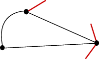
A half-edge is represented by a line incident to a unique vertex and without forming a loop. (See Figure 1.)
A half-edge incident to a unique vertex.

A HEG and its set
 $\mathfrak{f}^0$
of half-edges in red.

Definition 2.3 (Half-edged graph (HEG)). A HEG
 $G(\mathcal{V},\mathcal{E},\mathfrak{f}^0)$
or more briefly
 $G_{\mathfrak{f}^0}$
is a graph
 $G(\mathcal{V},\mathcal{E})$
with a set
 $\mathfrak{f}^0$
, whose elements are called half-edges together with a relation which associates with each half-edge a unique vertex. (See Figure 2.) The graph G is called the underlying graph of
 $G_{\mathfrak{f}^0}$
.
From the above definition, it is direct to observe that an abstract graph is a HEG with
 $\mathfrak{f}^0=\emptyset$
.
Definition 2.4 (Cut of an edge [Reference Krajewski, Rivasseau, Tanasa and Wang24]). Let
 $e \in \mathcal{E}$
be an edge of
 $G(\mathcal{V},\mathcal{E},\mathfrak{f}^0)$
. The cut HEG
 $G_{\mathfrak{f}^0}\vee e$
is obtained from
 $G_{\mathfrak{f}^0}$
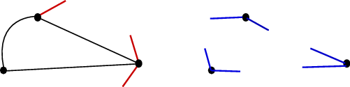
by cutting e, namely by deleting e and attaching a half-edge to each of the end vertices of e. Two half-edges are attached to the same vertex if e is a loop. (See Figure 3.) We denote by
 $\mathfrak{f}^1$
the set of half-edges that result from cutting all edges in
 $\mathcal{E}$
, and write
 $\mathfrak{f}$
for
 $\mathfrak{f}^0 \dot{\cup}\mathfrak{f}^1$
. (See an illustration in Figure 4.)
Cutting an edge.

A HEG (on the left), its set
 $\mathfrak{f}^0$
of half-edges in red, and set
 $\mathfrak{f}^1$
in blue obtained by cutting all its edges and removing
 $\mathfrak{f}^0$
.

Definition 2.5 (Spanning c-subgraphs of a HEG). A spanning c-subgraph A of
 $G(\mathcal{V},\mathcal{E},\mathfrak{f}^0)$
is the result of taking a spanning subgraph of
 $G(\mathcal{V},\mathcal{E})$
viewing it as embedded in
 $G(\mathcal{V},\mathcal{E},\mathfrak{f}^0)$
, then cutting all the edges of
 $\mathcal{E}{\setminus}\mathcal{E}_A$
. More precisely, a spanning c-subgraph A of
 $G(\mathcal{V},\mathcal{E},\mathfrak{f}^0)$
is defined as a HEG
 $A(\mathcal{V}_A,\mathcal{E}_A,\mathfrak{f}^0_A)$
, the edge set
 $\mathcal{E}_A$
of which is a subset of
 $\mathcal{E}$
with all vertices and all additional half-edges of
 $G_{\mathfrak{f}^0}$
. Hence
 $\mathcal{E}_A\subseteq \mathcal{E}$
,
 $\mathcal{V}_A = \mathcal{V}$
, and
 $\mathfrak{f}^0_A = \mathfrak{f}^{0} \cup \mathfrak{f}^{1}_A(\mathcal{E}_A)$
, where
 $\mathfrak{f}^{1}_A (\mathcal{E}_A)$
is the set of half-edges obtained by cutting all edges in
 $\mathcal{E}{\setminus}\mathcal{E}_A$
. We denote it
 $A \Subset G_{\mathfrak{f}^0}$
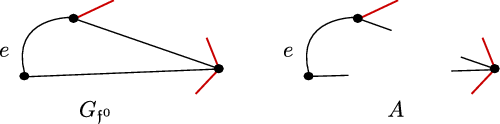
. (See A as an illustration in Figure 5.)
A HEG
 $G_{\mathfrak{f}^0}$
and the spanning c-subgraph A associated with e.

The isomorphism class of HEGs follows the same idea of that of abstract graphs. The sets of half-edges in the same class of HEGs must be of the same cardinality and satisfy the same incidence relation onto vertices.
Note that a spanning c-subgraph
 $A \Subset G_{\mathfrak{f}^0}$
, unless
 $A =G_{\mathfrak{f}^0}$
, has always a greater number of half-edges than
 $G_{\mathfrak{f}^0}$
. The rank and nullity of a HEG
 $G_{\mathfrak{f}^0}$
are defined to be the rank and nullity of the underlying graph G:
 $r(G_{\mathfrak{f}^0})= r(G)$
,
 $n(G_{\mathfrak{f}^0})=n(G)$
. Deleting an edge e in a HEG
 $G_{\mathfrak{f}^0}$
is deleting it from its underlying graph while keeping all half-edges and their incidence relation. We denote it in the standard way
 $G_{\mathfrak{f}^0}-e$
.
Definition 2.6 (Edge contraction of HEG). Let
 $G(\mathcal{V},\mathcal{E},\mathfrak{f}^0)$
be a HEG. We define the contraction of a non-loop edge e in
 $G_{\mathfrak{f}^0}$
, i.e.
 $G_{\mathfrak{f}^0}/e$
to be the HEG obtained from
 $G_{\mathfrak{f}^0}$
by removing e and identifying the two end vertices into a new vertex having all their additional half-edges and remaining incident lines. For a loop e, contraction
 $G_{\mathfrak{f}^0}/e$
and deletion
 $G_{\mathfrak{f}^0}-e$
coincide.
Noting that the edge contraction does not change the number of additional half-edges in a HEG, the following proposition is straightforward.
Proposition 2.7. Let
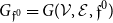 $G_{\mathfrak{f}^0}=G(\mathcal{V},\mathcal{E}, \mathfrak{f}^0)$
be a HEG and e one of its edge. Then
 $G_{\mathfrak{f}^0}/e=(G_{\mathfrak{f}^0}/e)(\mathcal{V}', $
 $\mathcal{E}{\setminus} \{e\}, \mathfrak{f}^0)$
, where
 $\mathcal{V}'$
is the set of vertices of the underlying abstract graph
 $G/e$
, and
 $G_{\mathfrak{f}^0}\vee e=(G_{\mathfrak{f}^0}\vee e)$
 $(\mathcal{V},\mathcal{E}{\setminus} \{e\}, \mathfrak{f}^0 \cup \{e_1,e_2\})$
, where
 $e_{1}$
and
 $e_2$
are the two half-edges obtained by cutting e.
The disjoint union and one-point join of HEGs are defined as for graphs carrying the half-edges along. Spanning c-subgraphs of
 ${G_1}_{\mathfrak{f}_1^0} \sqcup {G_2}_{\mathfrak{f}_2^0}$
and of
 ${G_1}_{\mathfrak{f}_1^0} \cdot_{v_1,v_2} {G_2}_{\mathfrak{f}_2^0}$
are of the form
 $A_{1} \sqcup A_{2}$
and
 $A_{1}\cdot_{v_1,v_2} A_{2}$
, respectively, with
 $A_i \Subset {G_i}_{\mathfrak{f}^0_i}$
,
 $i=1,2$
. The spanning c-subgraphs of
 ${G_1}_{\mathfrak{f}_1^0}\sqcup {G_2}_{\mathfrak{f}_2^0}$
and of
 ${G_1}_{\mathfrak{f}_1^0} \cdot_{v_1,v_2} {G_2}_{\mathfrak{f}_2^0}$
are thus in one-to-one correspondence.
2.3 A Tutte polynomial for HEGs
We extend the Tutte polynomial to HEGs and determine some properties of the new function.
Definition 2.8 Let
 $G_{\mathfrak{f}^0}$
be a HEG and G its underlying graph. Then
 \begin{equation} \mathcal{T}_{G_{\mathfrak{f}^0}}(x,y,t)=t^{|\mathfrak{f}^0|+2n\left(G_{\mathfrak{f}^0}\right)} \,T_{G}\left(X, \frac{Y}{t^2}\right) \,,\end{equation}
where
 $X=t^2(x-1) + 1$
and
 $Y=y +t^2-1$
.
The particular expressions for X and Y were determined to get a simplified form of the following properties.
Proposition 2.9. The function
 $\mathcal{T}$
has the following properties for a HEG
 $H= G_{\mathfrak{f}^0}$
, analogous to those of the Tutte polynomial for graphs.
a.
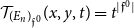 $\mathcal{T}_{(E_n)_{\mathfrak{f}^0}}(x,y,t) = t^{|\mathfrak{f}^0|}$
, where
 $(E_n)_{\mathfrak{f}^0}$
is the HEG with n vertices, no edges and
 $|\mathfrak{f}^0|$
half-edges.
b.
 \begin{eqnarray}\mathcal{T}_{H}= \left\{\begin{array} {lr} X\mathcal{T}_{H-e}(x,y,t) & \text{if e is a bridge,}\\
Y \mathcal{T}_{H/e} (x,y,t) & \text{if e is a loop,} \\ t^2 \mathcal{T}_{H-e} (x,y,t) + \mathcal{T}_{H/e}(x,y,t) & \text{if e is ordinary;}\end{array}\right.\end{eqnarray}
c.
 \begin{equation}\mathcal{T}_{H} =\mathcal{T}_{H \vee e} (x,y,t) + \mathcal{T}_{H/e}(x,y,t) \quad \text{if e is ordinary;}\end{equation}
d.
 \begin{equation}\mathcal{T}_{H} (x,y,t) =\sum_{A\Subset H}(x-1)^{r(H)-r(A)}(y-1)^{n(A)} \,t^{|\mathfrak{f}^0(A)|}\,.\end{equation}
Properties (a) and (b) follow immediately from Definition 2.2, using the usual additive properties of the rank for bridges, loops and ordinary edges, and noting that
 $|\mathfrak{f}^0(H)|=|\mathfrak{f}^0(H-e)|=|\mathfrak{f}^0(H/e)|$
.
For property (c), note that
 $H \vee e$
is just
 $H-e$
with the addition of two half-edges appended to the end points of e, so that
 $\mathcal{T}_{H\vee e}(x,y,t)= t^2 \mathcal{T}_{H-e}(x,y,t)$
.
To prove property (d), we use Definition 2.1, substituting the expressions for X and Y given in (3), and noting that there is a one-to-one correspondence between the spanning subgraphs of
 $H=G_{\mathfrak{f}^0}$
and G, and that
 $|\mathfrak{f}^0(A)|=|\mathfrak{f}^0|+2|\mathcal{E}|-2|\mathcal{E}_A|$
.

Note that property (c) can replace the third term of property (b) suggesting that cut may be a more natural operation on HEGs than deletion. The polynomial
 $\mathcal{T}_{G_{\mathfrak{f}^0}}$
has always a factor of
 $t^{|\mathfrak{f}^{0}|}$
which may be removed by a new normalization. The exponent of t in
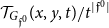 $\mathcal{T}_{G_{\mathfrak{f}^0}}(x,y,t)/t^{|\mathfrak{f}^0|}$
is always even since each c-spanning subgraph is defined via successive cut of edges yielding each two half-edges. The polynomial of the terminal form of a HEG with m bridges, n loops and q additional half-edges is
 \begin{equation} \left( 1+ (x-1)t^2\right)^m\, \left(y-1 + t^2\right)^n \,t^q=X^m Y^n t^q\,.\end{equation}
For
 $G_{1 \mathfrak{f}^0_1}$
and
 $G_{2 \mathfrak{f}^0_2}$
two HEGs, then it is immediate to get
 \begin{eqnarray}\mathcal{T}_{G_{1 \mathfrak{f}^0_1} \sqcup G_{2 \mathfrak{f}^0_2}}= \mathcal{T}_{G_{1 \mathfrak{f}^0_1}} \mathcal{T}_{G_{2 \mathfrak{f}^0_2}} = \mathcal{T}_{G_{1 \mathfrak{f}^0_1} \cdot_{v_1,v_2} G_{2 \mathfrak{f}^0_2}}\,,\end{eqnarray}
for any vertices
 $v_{i}$
in
 $G_{i \mathfrak{f}^0_i}$
,
 $i=1,2$
, from the properties (2) and (3), and because the number of half-edges and nullity are additive on disconnected graphs. Putting
 $t=1$
in
 $\mathcal{T}_{G_{\mathfrak{f}^0}}(x,y,t)$
yields the ordinary Tutte polynomial
 \begin{equation}\mathcal{T}_{G_{\mathfrak{f}^0}}(x,y,1)=T_{G}(x,y)\,.\end{equation}
3. Ribbon graphs and the BR polynomial
In this section, we first recall the generalization of the Tutte polynomial to ribbon graphs known as the BR polynomial for ribbon graphs, following the notation of [Reference Bollobás and Riordan9, Reference Bollobás and Riordan10]. Then, we investigate ribbon graphs with half-edges, or half-ribbons, analogous to the HEGs of Subsection 2.2.
3.1. Ribbon graphs
We recall basics of ribbon graphs and the BR polynomial according to conventions of [Reference Bollobás and Riordan10]. Note that the following axioms are equivalent to those of [Reference Reshetikhin and Turaev26].
Definition 3.1 (Ribbon graphs). A ribbon graph
 $\mathcal{G}$
is a (not necessarily orientable) surface with boundary represented as the union of two sets of closed topological discs called vertices
 $\mathcal{V}$
and edges
 $\mathcal{E}.$
These sets satisfy the following:
-
• vertices and edges intersect in disjoint line segments,
-
• each such line segment lies on the boundary of precisely one vertex and one edge,
-
• every edge contains exactly two such line segments.
Defining the class of ribbon graphs we are considering, we follow conventions of [Reference Bollobás and Riordan9, Reference Bollobás and Riordan10, Reference Ellis-Monaghan and Moffatt16]. The following description of ribbon graphs, known as rotation systems, is dated back to [Reference Heffter22]. A signed rotation system is a graph G together with a cyclic ordering of the edges at each vertex of G, and an assignment of a sign
 $+$
or minus; to each edge of G. The flip of a vertex v is an operation on the signed rotation system which reverses the cyclic order of the edges incident to v and switches all signs of edges incident to v, except the signs of its loops (edges incident to the same vertex). Two rotation systems are equivalent if they can be transformed by a sequence of vertex flips composed by graph isomorphisms.
There is an equivalence between signed rotation systems and ribbon graphs. To make this equivalence manifest, consider a ribbon graph
 $\mathcal{G}$
, choose an orientation on each vertex, and assign to each edge an orientation according to the fact that the orientation of its end vertices across the edge are consistent or not, respectively. The underlying graph G of
 $\mathcal{G}$
with the vertex and edge orientations is a signed rotation system (the initial choice of orientations for the vertex and edges of
 $\mathcal{G}$
does not matter in the construction of the signed rotation system because the latter is stable under vertex flips). Given now a rotation system G, we can construct a ribbon graph from G by replacing its vertices by discs, giving each disc an orientation, and attaching ribbon edges to these discs in the order given by the cyclic order of the vertices of G. A ribbon edge has an orientation: if this orientation is
 $+$
, the ribbon edge is attached with both the ends in a consistent way with the orientation of its end vertices, otherwise, if the orientation is minus;, then exactly one end is attached consistently with one end vertex. We call ribbon edges with a
 $+$
sign positive and negative, otherwise.
If the notions of ordinary ribbon edges and bridges need no comment, that of loops in ribbon graphs needs careful attention. A loop is a ribbon edge incident to the same vertex. A loop e at a vertex v is called trivial if there is no cycle in
 $\mathcal{G}$
which can be contracted to form a loop f at v such that the ends of e and f alternate in the cyclic order at v (see again [Reference Bollobás and Riordan10]).
We can address now the notion of contraction and deletion of ribbon edges. The following operations on ribbon graphs can be found detailed and illustrated in [Reference Bollobás and Riordan10]. Let
 $\mathcal{G}$
be a ribbon graph and e one of its edges. We call
 $\mathcal{G}-e$
the ribbon graph obtained from
 $\mathcal{G}$
by deleting e. If e is not a loop, consider its end vertices
 $v_1$
and
 $v_2$
. The graph
 $\mathcal{G}/e$
obtained by contracting e is defined from
 $\mathcal{G}$
by replacing e,
 $v_1$
and
 $v_2$
by a single vertex disc
 $e\cup v_1 \cup v_2$
. We now suppose that e is a loop and is incident to a unique vertex v. Two situations may occur: either
 $e\cup v$
forms a M
 ${\ddot{\textrm{o}}}$
bius band (trivial negative loop) with a single boundary cycle, or an annulus (trivial positive loop) with two boundary cycles. If
 $e\cup v$
forms a trivial negative loop, the graph
 $\mathcal{G}/e$
is obtained from
 $\mathcal{G}$
by deleting e and v and adding one new vertex whose boundary is the boundary of
 $e \cup v$
. If e is a trivial positive loop, the contraction of e is the deletion of e and v and the addition of two vertices, the union of whose boundaries is the boundary of
 $e \cup v$
. In this case, the operation at a vertex v splits the cyclic order at v into two cycles, which may represent two vertices into which v is split. We must emphasize that this operation of contraction should preserve the incidence and cyclic ordering of the remaining edges of the graph.
We use the following terminology:
Definition 3.2 (Faces). Consider
 $\mathcal{G}$
a ribbon graph as a surface with boundary. A face is a boundary component of
 $\mathcal{G}$
.
Ribbon graphs are known to be equivalent to graphs cellularly embedded in surfaces, see for instance [Reference Ellis-Monaghan and Moffatt16]. A face of a ribbon graph uniquely corresponds to a face of the embedding. In the next subsections, after introducing more combinatorial definitions, the notion of face might refer to a combinatorial object different from the usual connected component of the boundary of a ribbon graph.
Spanning subgraphs in this context are denoted again as
 $A \Subset \mathcal{G}$
. We are in position to define the BR polynomial.
Definition 3.3 (BR polynomial [Reference Bollobás and Riordan10]). Let
 $\mathcal{G}$
be a ribbon graph. The BR polynomial of
 $\mathcal{G}$
is an element of
 $\mathbb{Z}[x,y,z,w]$
quotiented by the ideal generated by
 $w^2-w$
, given by:
 \begin{equation}R_{\mathcal{G}}(x,y,z,w) =\sum_{A\Subset \mathcal{G}} (x-1)^{r(\mathcal{G})-r(A)}(y-1)^{n(A)}z^{k(A)-F(A)+n(A)} w^{o(A)},\end{equation}
where F(A) is the number of faces of A, and where
 $o(A)=0$
if A is orientable, and
 $o(A)=1$
if not.
In [Reference Bollobás and Riordan10], it is proved that the BR polynomial also obeys a contraction and deletion rule for ordinary edges as
 \begin{equation}R_{\mathcal{G}}=R_{\mathcal{G}/e}+ R_{\mathcal{G}-e}\,.\end{equation}
Also, for every bridge e of
 $\mathcal{G}$
, we have
 \begin{equation}R_{\mathcal{G}}=x \, R_{\mathcal{G}/e}\,,\end{equation}
for a trivial positive loop,
 \begin{equation}R_{\mathcal{G}}=y \,R_{\mathcal{G}-e}\,,\end{equation}
and for a trivial negative loop, the following relation holds
 \begin{equation}R_{\mathcal{G}}=(1+(y-1)zw) \,R_{\mathcal{G}-e}\,.\end{equation}
The relations (12)–(14) are assimilated to boundary conditions for the contraction deletion recursion relation. These boundary conditions were extended to a larger family of one-vertex ribbon graphs in [Reference Avohou, Ben Geloun and Livine3]. Nevertheless, in contrast with the Tutte polynomial, the relations (11)–(14) and the like are not sufficient for computing the BR polynomial for arbitrary ribbon graphs after a series of contractions and deletions.
Take any positive integer valued function
 $h: \mathbb{N}^3 \to \mathbb{N}$
and replace exponent of z in Definition 3.3 by
 \begin{equation}h(k(A),F(A),n(A))\,.\end{equation}
One can show that (11) still holds for an ordinary edge. The choice
 $k(A) - F(A) + n(A)$
for the exponent of z is interesting because
 \begin{equation}k(A) - F(A) + n(A)= 2k(A) - (|\mathcal{V}| - |\mathcal{E}_A| - F(A))\end{equation}
is nothing but the genus or twice the genus (for oriented surfaces) of the subgraph A. Furthermore, writing the exponent in this form also helps for the determination of the terminal forms because
 $k(A) - F(A)$
and n(A) turn out to be additive quantities with respect to the one-point join of disjoint graphs. These remarks will be exploited to find a generalization of the BR polynomial to stranded graphs.
3.2. Half-edged ribbon graphs (HERGs)
We generalize the BR polynomial to ribbon graphs with half-edges or half-ribbons. For convenience, we use an idea by Chmutov in [Reference Chmutov14] who considers a ribbon edge as a rectangle incident to the corresponding vertices along a pair of its opposite sides.
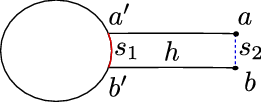
Definition 3.4 (Ribbon half-edges and external points). A ribbon half-edge (or simply half-ribbon, denoted henceforth HR) is a rectangle incident to a unique vertex of a ribbon graph by a unique line segment s on the boundary and without forming a loop. The segment parallel to s is called the external segment. The end points of any external segment are called external points of the HR. The two boundary segments of a ribbon edge or of a HR that are neither external nor incident to a vertex are called strands. A HR is always oriented consistently with the vertex it intersects.
A HR incident to a vertex is drawn in Figure 6. The next definition was introduced in [Reference Krajewski, Rivasseau and Vignes-Tourneret23]. We reformulate it according to our previous notation and definitions.
A HR h incident to a vertex disc. The two segments of h are
 $s_1$
intersecting the vertex and
 $s_2$
, the external segment with end points a and b. The strands of the HR are the segments [aa ′] and [bb ′].

Definition 3.5 (Cut of a ribbon edge). Let
 $\mathcal{G}$
be a ribbon graph and let e be a ribbon edge of
 $\mathcal{G}$
. The cut graph
 $\mathcal{G} \vee e$
is obtained from
 $\mathcal{G}$
by deleting e and attaching two HRs at the same line segments where e was incident to the end vertices, one at each of the end vertices of e. If e is a loop, the two HRs are on the same vertex.
Definition 3.6 A HERG
 $\mathcal{G}(\mathcal{V},\mathcal{E},\mathfrak{f}^0)$
(or simply
 $\mathcal{G}_{\mathfrak{f}^0}$
) is a ribbon graph
 $\mathcal{G}(\mathcal{V},\mathcal{E})$
(or shortly
 $\mathcal{G}$
) with a set
 $\mathfrak{f}^0$
of HRs such that each HR is attached to a unique vertex as in Definition 3.4, and the segments where the HRs are attached are disjoint from each other and from the segments where any ribbon edges are attached. The ribbon graph
 $\mathcal{G}$
is called the underlying ribbon graph of the HERG
 $\mathcal{G}_{\mathfrak{f}^0}$
.
The cut of a ribbon edge e in a HERG is the cut of e in its underlying ribbon graph. Using Definitions 2.5 and 3.6, spanning c-subgraphs of HERGs make sense. A spanning c-subgraph is then formed by cutting some subset of the ribbon edges. We denote again the spanning c-subgraph inclusion as
 $A \Subset \mathcal{G}_{\mathfrak{f}^0}$
. Note that a ribbon graph is a HERG with
 $\mathfrak{f}^0=\emptyset$
.
Considered as geometric surfaces, cutting an edge in a ribbon graph or in a HERG modifies the boundary of that surface. There are boundary components following the boundary of the HR. Combinatorially, we want to distinguish this type of face and those which uniquely follow the boundary of ribbon edges. This will be also useful in the following section when considering the case of stranded graphs. The combinatorial objects that are defined below were introduced in [Reference Gurau20]. We reformulate them using our conventions.
Definition 3.7 (Closed, open faces). Consider a HERG
 $\mathcal{G}_{\mathfrak{f}^0}$
.
-
• A closed face is a boundary component of
 $\mathcal{G}_{\mathfrak{f}^0}$
which never passes through any external segment of a HR. The set of closed faces is denoted
$\mathcal{F}_{{\textrm{int}}}$
. (See the closed face
$f_{1}$
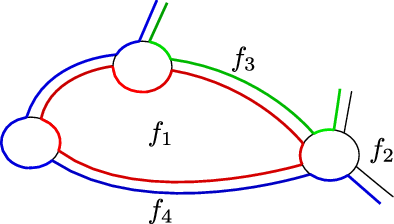
in Figure 7.)Figure 7.
A HERG with a closed face
$f_1$
(in red) and open faces
$f_{2}, f_{3},f_{4}$
(in black, green and blue, resp.). -
• An open face is a boundary arc leaving an external point of some HR rejoining another external point without passing through any external segment of a HR. The set of open faces is denoted
$\mathcal{F}_{{\textrm{ext}}}$
. (Examples of open faces are provided in Figure 7.) -
• The set of faces
$\mathcal{F}$
of a HERG is defined by
$\mathcal{F}_{{\textrm{int}}} \cup \mathcal{F}_{{\textrm{ext}}}$
.


Definition 3.8 (Boundary graph [Reference Gurau20]). The boundary graph
 $\partial{\mathcal{G}}_{\mathfrak{f}^0}$
of a HERG
 $\mathcal{G}_{\mathfrak{f}^0}$
is an abstract graph
 $\partial{\mathcal{G}}_{\mathfrak{f}^0}({\mathcal{V}}_{\partial},{\mathcal{E}}_{\partial})$
such that
 ${\mathcal{V}}_{\partial}$
is in one-to-one correspondence with
 $\mathfrak{f}^0$
, and
 ${\mathcal{E}}_{\partial}$
is in one-to-one correspondence with
 $\mathcal{F}_{{\textrm{ext}}}$
. Consider an edge e of
 ${\mathcal{E}}_{\partial}$
, its corresponding open face
 $f_e \in\mathcal{F}_{{\textrm{ext}}} $
, a vertex v, and its corresponding HR
 $h_v$
. The edge e is incident to v if and only if
 $f_e$
has one end point in
 $h_v$
, and, if both end points of
 $f_e$
are in
 $h_v$
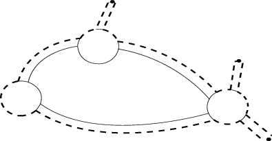
, then e is a loop. (The boundary of the graph given in Figure 7 is provided in Figure 8.)
The boundary graph
 $\partial{\mathcal{G}}_{\mathfrak{f}^0}$
of
 $\mathcal{G}_{\mathfrak{f}^0}$
of Figure 7 is the dashed cycle.

The boundary graph of a ribbon graph is empty. Note that
 $\partial{\mathcal{G}}_{\mathfrak{f}^0}$
is a disjoint union of cycles and also that the connected components of
 $\partial{\mathcal{G}}_{\mathfrak{f}^0}$
are in one-to-one correspondence with the faces of
 $\mathcal{G}$
that do not correspond to the closed faces of
 $\mathcal{G}_{\mathfrak{f}^0}$
.
The notion of edge contraction and deletion for HERGs can be simply understood as in the case of ribbon graphs. Let
 $\mathcal{G}_{\mathfrak{f}^0}$
be a HERG and
 $\mathcal{G}$
its underlying ribbon graph. In notation of Definition 3.3, we now define
 $r(\mathcal{G}_{\mathfrak{f}^0})=r(\mathcal{G}),\, n(\mathcal{G}_{\mathfrak{f} ^0})=n(\mathcal{G})$
,
 $o(\mathcal{G}_{\mathfrak{f}^0})=o(\mathcal{G})$
.
Definition 3.9 (BR polynomial for HERGs). Let
 $\mathcal{G}(\mathcal{V},\mathcal{E},\mathfrak{f}^0)$
be a HERG. We define the BR polynomial of
 $\mathcal{G}_{\mathfrak{f}^0}$
to be
 \begin{equation}\mathcal{R}_{\mathcal{G}_{\mathfrak{f}^0}}(x,y,z,s,w,t)=\sum_{A\Subset \mathcal{G}_{\mathfrak{f}^0}} (x-1)^{r(\mathcal{G}_{\mathfrak{f}^0})-r(A)}(y-1)^{n(A)}z^{k(A)-F_{{\textrm{int}}}(A)+n(A)} \, s^{C_\partial(A)} w^{o(A)}\, t^{\,f(A)},\end{equation}
where
 $F_{{\textrm{int}}}(A)= |\mathcal{F}_{{\textrm{int}}}(A)|$
,
 $C_\partial(A)= |{\mathcal{C}}_{\partial}(A)|$
is the number of connected components of
 $\partial A$
, the boundary graph of A,
 $o(A)=0$
if A is orientable, and 1 otherwise,
 $f(A)=|\mathfrak{f}^0(A)|$
is the number of HRs of A, and where
 $w^2=w$
holds.
The polynomial
 $\mathcal{R}$
(17) generalizes the BR polynomial R (10). R can be recovered from
 $\mathcal{R}$
using
 \begin{equation}\mathcal{R}_{\mathcal{G}_{\mathfrak{f}^0}}(x,y,z,z^{-1},w,t=1) =R_{\mathcal{G}}(x,y,z,w)\,.\end{equation}
The graph operations of disjoint union and one-point join extend to ribbon graphs and to HERGs. The one-point join
 $\mathcal{G}_{1\mathfrak{f}_1^{0}} \cdot_{v_1,v_2}\mathcal{G}_{2\mathfrak{f}_2^{0}}$
of disjoint HERGs
 $\mathcal{G}_{1\mathfrak{f}_1^{0}}$
and
 $\mathcal{G}_{2\mathfrak{f}_2^{0}}$
is obtained by choosing two vertices
 $v_1$
and
 $v_2$
of
 $\mathcal{G}_{1\mathfrak{f}_1^{0}}$
and
 $\mathcal{G}_{2\mathfrak{f}_2^{0}}$
, respectively, and merging
 $v_1$
and
 $v_2$
on an arc of each of these which does not contain any ribbon edges or HRs. Combinatorially, we must respect the cyclic order of all ribbon edges and HRs on the previous vertices
 $v_1$
and
 $v_2$
. It is well known that such a procedure might lead to non isomorphic ribbon graphs, see for instance [Reference Bollobás and Riordan10]. The fact that
 $R_{\mathcal{G}_1 \sqcup \mathcal{G}_2}= R_{\mathcal{G}_1} R_{\mathcal{G}_2} = R_{\mathcal{G}_1 \cdot_{v_1,v_2} \mathcal{G}_2}$
holds for ribbon graphs can be extended for HERGs under certain conditions.
We come to the properties of
 $\mathcal{R}_{\mathcal{G}_{\mathfrak{f}^0}}$
. The following proposition holds.
Proposition 3.10 (Union of HERGs). Let
 $\mathcal{G}_{1\mathfrak{f}^0_1} $
and
 $\mathcal{G}_{2\mathfrak{f}^0_2}$
be two disjoint HERGs, then
 \begin{equation}\mathcal{R}_{\mathcal{G}_{1\mathfrak{f}^0_1} \sqcup \mathcal{G}_{2\mathfrak{f}^0_2}} = \mathcal{R}_{\mathcal{G}_{1\mathfrak{f}^0_1} } \mathcal{R}_{\mathcal{G}_{2\mathfrak{f}^0_2}}\,.\end{equation}
Proof. It suffices to check the exponents for any
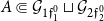 $A\Subset \mathcal{G}_{1\mathfrak{f}^0_1} \sqcup \mathcal{G}_{2\mathfrak{f}^0_2}$
. A spanning c-subgraph A of such a union of HERGs expresses as
 $A = A_1 \sqcup A_2 \Subset \mathcal{G}_{1\mathfrak{f}^0_1} \sqcup \mathcal{G}_{2\mathfrak{f}^0_2}$
with
 $A_{1} \Subset \mathcal{G}_{1\mathfrak{f}^0_1}$
and
 $A_{2} \Subset \mathcal{G}_{2\mathfrak{f}^0_2}$
. It is straightforward to see that k(A), r(A),
 $F_{{\textrm{int}}}(A)$
, n(A),
 $C_\partial(A)$
, and f(A) are all additive quantities. Furthermore,
 $o(A_1 \sqcup A_2)=\max\{o(A_1),o(A_2)\}$
, but
 $w^2=w$
. The result follows.
Theorem 3.11
(Contraction and cut for BR polynomial for HERGs) Let
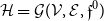 $\mathcal{H}= \mathcal{G}(\mathcal{V},\mathcal{E},\mathfrak{f}^0)$
be a HERG. Then, for an ordinary edge e,
 \begin{equation}\mathcal{R}_{\mathcal{H}}=\mathcal{R}_{ \mathcal{H}\vee e} +\mathcal{R}_{\mathcal{H}/e}\,,\end{equation}
for a bridge e, we have
 \begin{equation}\mathcal{R}_{\mathcal{H}} =(x-1)\mathcal{R}_{\mathcal{H} \vee e}+ \mathcal{R}_{\mathcal{H}/e}\,;\end{equation}
for a trivial negative loop e, the following holds
 \begin{equation}\mathcal{R}_{\mathcal{H}}=\mathcal{R}_{\mathcal{H} \vee e} + (y-1)zw \,\mathcal{R}_{\mathcal{H}/e}\,,\end{equation}
whereas for a trivial positive loop e, we have
 \begin{equation}\mathcal{R}_{\mathcal{H}}=\mathcal{R}_{\mathcal{H} \vee e} + (y-1) \mathcal{R}_{\mathcal{H}/e}\,.\end{equation}
Proof. In the following proof, spanning c-subgraphs are simply called subgraphs because no confusion can arise. Let us make two preliminary remarks. (A) The subgraphs A of
 $\mathcal{H}$
which do not contain e are precisely the subgraphs of
 $\mathcal{H}\vee e$
. (B) Also, if e is not a loop then the map
 $A\mapsto A/e$
provides a bijection from the subgraphs of
 $\mathcal{H}$
which contain e to the subgraphs of
 $\mathcal{H}/e$
that preserves closed faces as well as components of the boundary graph. Note importantly that, although A and
 $A/e$
do not have the same vertices and edges, they do have the same HRs and same faces.
Let us prove (20). For an ordinary edge e, let
 $A \Subset { \mathcal{H}}\vee e$
, and let A
′ be the corresponding subgraph in
 $\mathcal{H}$
such that
 $e \notin A'$
, by remark (A). The fact that the monomial of A in
 $\mathcal{R}_{{\mathcal{H}}\vee e}$
and the monomial corresponding to A
′ in
 $\mathcal{R}_{{ \mathcal{H}}}$
are identical is simple to check. Then
 $\sum_{A\Subset { \mathcal{H}}; e \notin A }$
 $(x-1)^{r({ \mathcal{H}})-r(A)}(y-1)^{n(A)}z^{k(A)-F_{{\textrm{int}}}(A)+n(A)} \, s^{C_\partial(A)} w^{o(A)}\, t^{\,f(A)} = \mathcal{R}_{{ \mathcal{H}}\vee e}$
.
We now concentrate on the remaining sum related to the contraction of e. In particular, we focus on the sets of faces during the contraction. Choose
 $A\Subset { \mathcal{H}}$
with
 $e \in A$
and, by remark (B), let
 $A' \Subset { \mathcal{H}}/e$
be its corresponding subgraph. One has
 \begin{eqnarray}F_{{\textrm{int}}}(A)=F_{{\textrm{int}}}\big(A'\big)\,,\; C_\partial(A)=C_\partial\big(A'\big) \,,\;o(A)= o\big(A'\big)\,,\,\mbox{ and } \,\, f(A) = f\big(A'\big) \,.\end{eqnarray}
The monomial of
 $\mathcal{R}_{{ \mathcal{H}}/e}$
related to A
′ is of the form
 \begin{align}&(x-1)^{r({ \mathcal{H}}/e) \,-\, r\big(A'\big)} (y-1)^{n\big(A'\big)}z^{k\big(A'\big)\,-\,F_{{\textrm{int}}}\big(A'\big)\,+\,n\big(A'\big)} \, s^{C_\partial\big(A'\big)} \, w^{o\big(A'\big)} t^{\,f\big(A'\big)}\nonumber\\[2pt]
&= (x-1)^{r({ \mathcal{H}})\,-\,1\, -\, (r(A)-1)} (y-1)^{n(A)} z^{k(A)\,-\,F_{{\textrm{int}}}(A)\,+\,n(A)} w^{o(A)}\, s^{C_\partial(A)} \, t^{\,f(A)}\end{align}
which achieves the proof that
 $\mathcal{R}_{{ \mathcal{H}}/e}=\sum_{A \Subset { \mathcal{H}}; e\in A} (x-1)^{r({ \mathcal{H}}/e) \,-\, r(A)} (y-1)^{n(A)}z^{k(A)\,-\,F_{{\textrm{int}}}(A)\,+\,n(A)} $
 $ s^{C_\partial(A)}w^{o(A)} t^{\,f(A)}$
, and then (20) holds.
We now focus on (21). Let e be a bridge in
 ${ \mathcal{H}}$
. Decompose
 $\mathcal{R}_{{ \mathcal{H}}}$
as
 \begin{equation}\sum_{A\Subset { \mathcal{H}}; e \notin A }(x-1)^{r({ \mathcal{H}})\,-\,r(A)}(y-1)^{n(A)}z^{k(A)-F_{{\textrm{int}}}(A)\,+\,n(A)} \, s^{C_\partial(A)} w^{o(A)}\, t^{\,f(A)}+ \mathcal{R}_{{ \mathcal{H}}/e}\,.\end{equation}
It remains to prove that the first sum corresponds to
 $(x-1)\mathcal{R}_{{ \mathcal{H}} \vee e}$
but this is straightforward from
 $r({ \mathcal{H}}) = r({ \mathcal{H}}\vee e)+1$
and since all other terms remain unchanged.
The proofs of relations (22) and (23) are now given. Consider a trivial (positive or negative) loop e in
 ${ \mathcal{H}}$
, then
 $\sum_{A\Subset { \mathcal{H}}; e \notin A }(x-1)^{r({ \mathcal{H}})\,-\,r(A)}(y-1)^{n(A)}z^{k(A)\,-\,F_{{\textrm{int}}}(A)\,+\,n(A)} \, s^{C_\partial(A)} w^{o(A)}\, t^{\,f(A)} =\mathcal{R}_{{ \mathcal{H}} \vee e}$
still holds in any case. The mapping from the subgraphs of
 ${ \mathcal{H}}$
containing e to those of
 ${ \mathcal{H}}-e$
, or conversely, is just obtained by deleting e or gluing e to the corresponding subgraph.
Consider a trivial negative loop e in
 $\mathcal{H}$
. To each
 $A\Subset \mathcal{H}$
such that
 $e \in A$
and its corresponding
 $A' \Subset \mathcal{H}/e$
, we find that
 $n(A)=n\big(A'\big)+1$
,
 $F_{{\textrm{int}}}(A) = F_{{\textrm{int}}}\big(A'\big)$
, and
 $C_\partial(A) = C_\partial\big(A'\big)$
. Therefore, we get the following relation between the terms:
 \begin{align}
&(x-1)^{r(\mathcal{H}) \,-\,r (A) } (y-1)^{n(A)} z^{k(A)\,-\,F_{{\textrm{int}}}(A)\,+\,n(A)} \, s^{C_\partial(A)} \,w^{o(A)}\, t^{\,f(A)}\nonumber\\
&\quad = (x-1)^{r(\mathcal{H}/ e) \,-\,r \big(A'\big) } (y-1)^{n\big(A'\big)\,+\,1} z^{k\big(A'\big)\,-\,F_{{\textrm{int}}}\big(A'\big)\,+\,n\big(A'\big)\,+\,1} \, s^{C_\partial\big(A'\big)}\,w^{o\big(A'\big)\,+\,1} \, t^{\,f\big(A'\big)}\,.\end{align}
Thus (22) is satisfied.
We now suppose that e is a trivial positive loop. With
 $A\Subset \mathcal{H}$
such that
 $e \in A$
, we associate a unique corresponding element A
′ in
 $ \mathcal{H} /e$
. We can infer that
 $k(A)=k\big(A'\big)-1$
,
 $n(A)=n\big(A'\big)+1$
,
 $F_{{\textrm{int}}}(A) = F_{{\textrm{int}}}\big(A'\big)$
, and
 $C_\partial(A) = C_\partial\big(A'\big)$
. Thus, the following relation between the terms corresponding to A and A
′ holds:
 \begin{eqnarray}&&(x-1)^{r(\mathcal{H}) -r (A) } (y-1)^{n(A)} z^{k(A)-F_{{\textrm{int}}}(A)+n(A)} \, s^{C_\partial(A)}\, w^{o(A)} \, t^{\,f(A)} \\ && (x-1)^{r(\mathcal{H}/e) -r \big(A'\big) } (y-1)^{n\big(A'\big)+1} z^{(k\big(A'\big)-1) - F_{{\textrm{int}}}\big(A'\big)+(n\big(A'\big)+1)} \, s^{C_\partial\big(A'\big)} \, w^{o\big(A'\big)}\, t^{\,f\big(A'\big)}\,,\end{eqnarray}
so that (23) is obtained.
Observe that, as in the case of the of the BR polynomial for ribbon graphs, Theorem 3.11 is not a complete reduction, since one-vertex HERGs with nontrivial loops must still be computed from (17). Given
 $\mathcal{G}_{\mathfrak{f}^0}$
a HERG and
 $\mathcal{G}$
its underlying ribbon graph, we also note the reduction
 \begin{equation}\mathcal{R}_{\mathcal{G}_{\mathfrak{f}^0}}(x,y,z,s=z^{-1},w,t) = t^{|\mathfrak{f}^0| + 2n(\mathcal{G})}R_{\mathcal{G}}(X,\frac{Y}{t^2},z,w)\end{equation}
where, once again,
 $X=t^2(x-1)+1$
and
 $Y=y+t^2-1$
.
4. Rank D half-edged stranded graphs and a generalized polynomial invariant
This section investigates the definition of a new polynomial for particular graphs which aims at generalizing the BR polynomial
 $\mathcal{R}$
for HERGs. The main notion of graphs discussed below is combinatorial and can be always pictured in a 3D space. Our main result appears in Theorem 4.32 after defining the generalized graphs we are dealing with.
The notion of rank D coloured tensor graphs considered here has been introduced by Gurau in [Reference Gurau17]. Using a duality, it is well known that ribbon graphs can be mapped onto triangulations of surfaces. In a similar way, coloured tensor graphs can be interpreted as simplicial complexes or dual of triangulations of topological spaces in any dimension. They are of particular interest in certain quantum field theories defined with tensor fields hence the name tensor graphs (ribbon graphs are, in this sense, rank 2 or matrix graphs). The importance of these graphs has been highlighted by Gurau in [Reference Gurau18] where that author proved that coloured tensor graphs have a cellular structure which associates each coloured tensor graph with a simplicial pseudo-manifold of D dimensions. It has been also proved that a coloured tensor graph which is bipartite induces naturally an orientation of the dual simplicial complex in [Reference Caravelli13].
Some previous studies have addressed the generalization of the BR polynomial for higher dimensional objects within the framework of such graphs. Mainly, two authors, Gurau in [Reference Gurau20] and Tanasa in [Reference Tanasa28], have defined two distinct notions of generalized BR polynomials. Let us give a brief review of their results and compare these to the one obtained in the present work.
Gurau defined a multivariate polynomial invariant for coloured tensor graphs associated with simplicial complexes with boundaries in any dimension D. The polynomial that we obtain in the present work can be put in a multivariate form which is related to Gurau’s polynomial restricted to 3D. Our polynomial extends Gurau’s polynomial to a class larger than coloured tensor graphs. We emphasize that the difficulties encountered by Gurau (as well as Tanasa, see below) for defining a contraction procedure for such type of graphs without destroying the entire graph structure is much improved in our scheme.
In a different perspective, the work by Tanasa in [Reference Tanasa28] deals with tensor graphs without colours that are equipped with another stranded vertex. The polynomial as worked out by this author is only valid for graphs triangulating topological objects without boundary. The polynomial that we define is radically different from that one in several features, since mainly, it relies on a graph colouring.
In another close related setting dealing with simplicial complexes, Krushkal and Renardy in [Reference Krushkal and Renardy25] identified a 4-variable polynomial invariant for triangulations and handle decompositions of orientable manifolds reducing to the BR polynomial. This polynomial might agree with the one that we will define for closed triangulations after specializing to 1 all variables related to the boundary of the complex. This deserves as well to be fully addressed elsewhere.
4.1. Stranded, tensor, coloured graphs with half-edges
Like ribbon graphs, coloured tensor graphs have both a topological meaning (realized in the dual triangulation) and a combinatorial formulation that is our main concern here. Before reaching the definition of coloured tensor graphs, we must introduce the combinatorial concept of stranded graphs, the true backbone of this theory.
Stranded and tensor graphs. We start by basic notions of stranded objects.
Definition 4.1 (Stranded vertex and edge). Let D be an integer,
 $D \ge 0$
.
-
• A stranded pre-vertex of rank
$D\ge 1$
consists of a set S of 2n elements called (vertex) points, together with two partitions of S: one into non-empty parts of size at most D, called pre-edges, and one into pairs, called chords. A rank
$D=0$
stranded vertex consists of a set S with a single or no element, and no partition of S (then there are no pre-edges or chords). The case
$n=0$
is allowed (then there are no pre-edges, or chords), and the resulting stranded pre-vertex is called a trivial circle which, by convention, we consider of any rank
$D \ge 0$
. The coordination number of v is the number of pre-edges in v. We say that a stranded pre-vertex v is disconnected if we can partition the set S into non-empty parts
$S_1$
and
$S_2$
such that no pre-edge or chord contains elements of both
$S_1$
and
$S_2$
, otherwise, v is connected. A rank D stranded vertex is a rank D stranded pre-vertex that is connected. -
• The vertex graph of a rank D stranded pre-vertex is the graph whose vertex set is the set of pre-edges and with one edge for each chord. The edge is incident to two vertices (or one in a loop case), corresponding to the two pre-edges (or one in a loop case) that contain the two paired points.
-
• A stranded edge of rank
$D\ge 1$
consists of a set S of 2D elements called (edge) points, together with two partitions, one into two sets of size D called ends, and one into D sets of size 2 called strands, each strand containing one point from each end.


Note that a stranded vertex is a stranded pre-vertex whose vertex graph is connected.
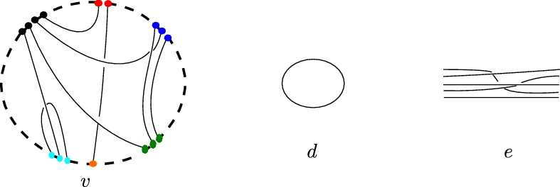
In the rest of this work, we use a particular realization for drawing stranded vertices and edges which does not play any important role. The chords of stranded vertices (resp. strands of stranded edges) are represented line segments that do not intersect and their crossings are irrelevant. The end points of chords are partitioned into sets representing the pre-edges with
 $1,2,\dots$
or D points. These points are drawn on a single arc of a fictitious circle, called the vertex frontier, with no other end points on this arc. Drawn in dash or dots, or as a solid circle when no confusion can arise, the vertex frontier is used to separate in drawings stranded vertices and edges in the (yet to be defined) stranded graphs. The cyclic order around the dotted circle does not matter, and this circle plays a different role from the vertex circles in ribbon graphs. Examples of stranded vertices and edges with rank
 $D=4$
and
 $D=5$
have been provided in Figure 9.
Graphical representation of stranded vertices and edges: a rank 4 stranded vertex v of coordination 6 (left), with pre-edges (highlighted with different colours) with non intersecting chords; a trivial circle vertex d; a rank 5 stranded edge e with non parallel strands (right).

Definition 4.2 (Stranded and tensor graphs).
-
• A rank D stranded graph
$ \mathscr{G} = \mathscr{G} (\mathcal{V},\mathcal{E})$
consists of a set
$\mathcal{V}$
of disjoint rank D stranded vertices (i.e., with all vertex points distinct), a set
$\mathcal{E}$
of disjoint stranded edges (i.e., with all edge points distinct) of rank at most D, and an incidence map
$\phi$
(not usually written in the notation) from the set of edge points to the set of vertex points satisfying the following conditions:
$\phi$
is injective, and on each end of each stranded edge,
$\phi$
acts as a bijection to some pre-edge of some stranded vertex in
$\mathcal{V}$
. In other words, each end of each stranded edge is attached to a distinct pre-edge of the correct size, with the D strands in each rank D edge attached bijectively to the D points in the pre-edge. -
• A rank D tensor graph
$ \mathscr{G} $
is a rank D stranded graph such that the stranded vertices of
$ \mathscr{G} $
have a fixed coordination
$D+1$
and their pre-edges have a fixed cardinality D. All vertex graphs are
$K_{D+1}$
. The stranded edges of
$ \mathscr{G} $
are of rank D.


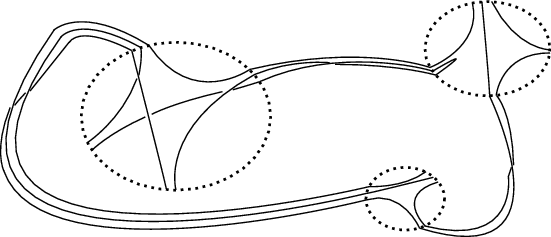
Some illustrations of a rank 3 stranded and tensor graphs are given in Figures 10 and 11, respectively.
A rank 3 stranded graph.

A rank 3 tensor graph with rank 3 stranded vertices as with fixed coordination 4, pre-edges with 3 points linked by chords according to the pattern of
 $K_4$
; stranded edges are rank 3.

It should be pointed out that, although the stranded vertices and edges of stranded and tensor graphs are drawn in a three dimensional space, we do not treat these as embedded graphs.
There are motivations for the introduction of tensor graphs. While stranded graphs can be treated as generalized graphs, tensor graphs, via a combinatorial duality, actually map to simplicial spaces. Consider
 $ \mathscr{G} $
a rank
 $D>0$
tensor graph. A stranded vertex of
 $ \mathscr{G} $
represents a D-simplex and the pre-edges are precisely their boundary
 $(D-1)$
-simplices. A stranded edge of
 $ \mathscr{G} $
represents the gluing of the D-simplex along one of their boundary
 $(D-1)$
-simplices. Hence, a tensor graph
 $ \mathscr{G} $
maps to a simplicial complex. As an illustration of the above combinatorial duality, a rank 3 tensor graph represents a simplicial complex in 3D composed by tetrahedra (3-simplex) which are glued along their boundary triangles (2-simplex). Such a duality has given a handle on the study of random simplicial manifolds in physics topics like quantum gravity [Reference Ambjorn, Durhuus and Jonsson1]. The interpretation of the circle vertices in the definition of tensor graphs can be done in the following convention: a trivial circle vertex in a rank
 $D \geq 2$
tensor graph represents a D dimensional ball.
Underlying graph and connectedness. Given a stranded graph
 $ \mathscr{G} $
and collapsing its stranded vertices to points and its stranded edges to simple lines, one obtains an abstract graph called underlying graph of
 $ \mathscr{G} $
. A stranded graph is connected if and only if its corresponding underlying graph is connected. For instance, both graphs of Figures 10 and 11 are connected since their underlying graphs coincide with the closed cycle graph
 $C_3$
.
Any rank D stranded graph is a rank D
′ stranded graph for any
 $D' \geq D$
. This is however not true for tensor graphs. In the following, the rank of a stranded graph refers to the minimal rank D for which this stranded graph is well defined.
Equivalence class of stranded graphs. Two stranded graphs are isomorphic if there are two bijections, one from the vertex points of the first to the vertex points of the second, and one from the edge points of the first to the edge points of the second, that preserve the structure, meaning the grouping into pre-edges, chords, edge ends and strands, as well as respecting the edge point to vertex point incidence maps. Furthermore these two graphs should have the same number of trivial circles.
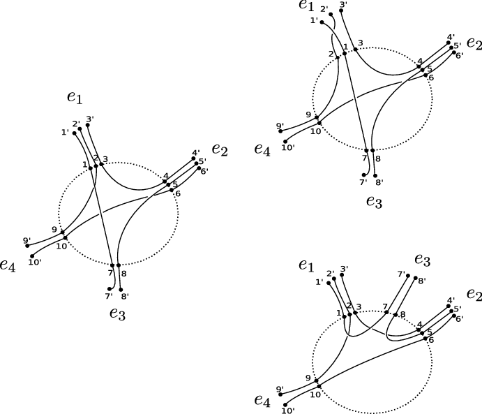
Figure 12 illustrates different ways of drawing part of the same stranded graph: the stranded vertex is defined by the pre-edges
 $\{1, 2, 3\}$
,
 $\{4, 5, 6\}$
,
 $\{7, 8\}$
,
 $\{9, 10\}$
and chords
 $\{1, 7\}$
,
 $\{2, 9\}$
,
 $\{3, 4\}$
,
 $\{5, 8\}$
,
 $\{6, 10\}$
and (in the edges) the strands are
 $\{i, i'\}$
;
 $i=1, \cdots, 10$
.
Different drawings of the same part of a stranded graph.

Low rank stranded graphs. As illustrations, we now discuss the lowest rank stranded graphs.
-
0. Rank 0 stranded or tensor graphs are abstract graphs made with only vertex points as rank 0 stranded vertices, no stranded edges, and possibly with trivial circles.
-
1. Rank 1 stranded/tensor graphs have both stranded vertices and edges like segments (possibly with additional trivial circles). Note that the connectivity condition implies that a rank 1 stranded vertex can only have
$n=0$
(hence is a trivial circle) or
$n=1$
(hence have two pre-edges of size 1). Such rank 1 stranded graphs cannot be directly identified with abstract graphs. Hence, neither rank 0 nor rank 1 stranded graphs define abstract graphs in general. Abstract graphs can be directly obtained from rank D stranded graph through the collapsing procedure described above, hence using the underlying graph. -
2. Ribbon graphs, in the sense of Definition 3.1, are in one-to-one correspondence with certain rank 2 stranded graphs. In the following, we show (a) how to construct the rank 2 stranded graph corresponding to a ribbon graph and (b) prove that two equivalent ribbon graphs lead to two equivalent rank 2 stranded graphs in the sense identified above.
-
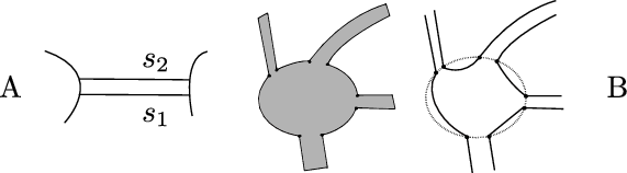
a. Let
$\mathcal{G}$
be a ribbon graph (Definition 3.1) and let e be an edge of
$\mathcal{G}$
. The ribbon edge e is incident to its end vertex (loop case) or vertices (ordinary case or bridge) in two segments s and s
′. Consider the two distinct segments on the boundary of e which are not s and s
′ (denoted by
$s_1$
and
$s_2$
in Figure 13A). These two segments define the two strands of a rank 2 stranded edge with s and s
′ as end segments. By convention, a circle is a stranded vertex in any rank, in particular
$D= 2$
, and so it is a stranded graph with no incident stranded edge. Consider now a vertex v of
$\mathcal{G}$
with incident edges
$e_1$
,
$e_2$
,
$\ldots,e_p$
,
$p \in \mathbb{N}$
. We can construct a stranded vertex v
′ of rank 2 from the data of v and of its incident ribbon edges in the following manner. Draw a fictitious circle as the frontier vertex of v
′. Insert on the frontier the end points of end segments of
$e_k$
,
$1\leq k \leq p$
, which define the pre-edges (with exactly 2 points) of v
′. From these pre-edges, one defines the chords of v
′ as the segments disposed cyclically between the end segments of
$e_k$
’s which lie in v. See Figure 13B. We stress again that the vertex frontier is totally virtual and is useful only for determining the separation between stranded edges and vertices. We can conclude that a rank 2 stranded graph obtained from a ribbon graph, in this way, is a combinatorial object defined on the boundary of the ribbon graph. -
b. Let us address now the issue of equivalent classes. It is obvious that equivalent ribbon graphs give rise to equivalent rank 2 stranded graphs. Now suppose that
$ \mathscr{G} _1$
and
$ \mathscr{G} _2$
are equivalent rank 2 stranded graphs arising from ribbon graphs
$\mathcal{G}_1$
and
$\mathcal{G}_2$
, respectively. We must show that the corresponding ribbon graphs are equivalent. The strands, chords, and points of
$ \mathscr{G} _1$
describe a 2-regular graph. Now add an edge between each pair of vertices that belong to the same pre-edge and obtain a 3-regular graph. Introduce a proper edge colouring of this cubic graph, according to the edge arises from a chord, a strand or a pre-edge. The resulting object is a description of
$\mathcal{G}_1$
as a graph encoded map (see, for instance [Reference Bonnington and Little11], p. 30, for background on graph encoded maps). Since equivalence of vertex stranded graphs does not change the arising graph encoded map,
$\mathcal{G}_1$
and
$\mathcal{G}_2$
must be equivalent ribbon graphs.
-


From the above analysis, ribbon graphs map to rank 2 stranded graphs. Nevertheless, it must be made clear that the converse is not true. To any rank 2 stranded graph, we cannot necessarily assign a ribbon graph (for several reasons, one of which is that, in rank 2 stranded graphs, pre-edges with a single point are allowed and this does not make sense in the context of ribbon graphs). Still from the previous analysis, we can immediately establish that ribbon graphs with vertices with fixed coordination equals to 3 are rank 2 tensor graphs. In that case, the converse is also true because, in any rank 2 tensor graph, we can always make cyclic a rank 2 vertex by a sequence of point permutations. The cyclic vertex and its incident 3 stranded edges (2 in presence of a loop) are one-to-one mapped with a disc with three incident ribbon edges (2 in presence of a loop). Studying in the following sections rank 2 stranded graphs, we will directly treat them as ribbon graphs.
Ribbon edge and vertex of a ribbon graph as a rank 2 stranded edge and vertex of a stranded graph (the frontier vertex appears in dash is fictitious).

Definition 4.3 (Half-edged stranded graphs (HESGs) and stranded half-edge (sHE)).
-
• A rank D half-edged stranded graph (HESG)
$ \mathscr{G} (\mathcal{V},\mathcal{E},\mathfrak{f}^0)$
(or more simply
$ \mathscr{G} _{\mathfrak{f}^0}$
) consists of a set
$\mathcal{V}$
of disjoint rank D stranded vertices, a set
$\mathcal{E}\cup\mathfrak{f}^0$
,
$\mathcal{E}\cap\mathfrak{f}^0 = \emptyset$
, of disjoint stranded edges of rank at most D, together with an incidence map
$\phi$
from the set of edge points to the set of vertex points satisfying the following conditions:
$\phi$
is defined on both ends of every edge in
$\mathcal{E}$
but only one end of each edge in
$\mathfrak{f}^0$
; on this set of edge points
$\phi$
is injective, and (as before) on each end of each stranded edge on which
$\phi$
is defined, it is a bijection to some pre-edge. Finally,
$\phi$
is a surjection onto all vertex points so that every pre-edge of every stranded vertex of has some end of some stranded edge of
$\mathcal{E}\cup\mathfrak{f}^0$
attached to it. -
• A rank d,
$ 0 \le d \le D$
, stranded edge in
$\mathfrak{f}^0$
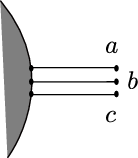
is called rank d stranded half-edge (sHE) since they are attached at one end. The edge points of the set of segment ends of a sHE which do not intersect the stranded vertex are called external points of the rank d sHE. (See Figure 14.)Figure 14.A rank 3 sHE with its external points a, b and c.
-
• Removing the set
$\mathfrak{f}^0$
of sHEs of a rank D HESG
$ \mathscr{G} _{\mathfrak{f}^0}$
, and using the proper restriction of
$\phi$
on the edge points from the ends of
$\mathcal{E}$
, we define a rank D stranded graph
$ \mathscr{G} $
called the underlying stranded graph of
$ \mathscr{G} _{\mathfrak{f}^0}$
.


We represent a rank D sHE by a set of D (parallel) line segments (see Figure 14). In a HESG
 $ \mathscr{G} _{\mathfrak{f}^0}$
with an empty set of sHEs,
 $\mathfrak{f}^0=\emptyset$
, every pre-edge is connected to a certain stranded edge.
It is obvious that a HESG
 $ \mathscr{G} _{\mathfrak{f}^0}$
may have trivial circles as stranded vertices if the stranded graph
 $ \mathscr{G} $
does have ones. An example of a HESG is given in Figure 15. A half-edged tensor graph is nothing but a HESG with stranded vertices and edges satisfying also the conditions of a tensor graph, see Definition 4.2.
A rank 3 HESG.

We can define the following edge operations on stranded graphs.
Definition 4.4 (Deletion and cut of a stranded edge). Let
 $ \mathscr{G} _{\mathfrak{f}^0}$
be a rank D HESG and e one of its rank d stranded edges,
 $1\leq d \leq D$
. The stranded graph
 $ \mathscr{G} _{\mathfrak{f}^0} - e$
is obtained from
 $ \mathscr{G} _{\mathfrak{f}^0}$
by deleting e.
The cut stranded graph
 $ \mathscr{G} _{\mathfrak{f}^0} \vee e$
is obtained from
 $ \mathscr{G} _{\mathfrak{f}^0}$
by cutting e that is by deleting e and attaching two rank d sHEs at the same pre-edge of the stranded vertices where e was incident, one at each of the end vertices of e. (See Figure 16.) If e is incident to a unique stranded vertex, the two sHEs are on the same vertex.
Cutting a rank 3 stranded edge.

The notion of spanning c-subgraph for HESGs follows naturally from Definition 2.5. The spanning c-subgraph inclusion is again denoted by
 $A \Subset \mathscr{G}_{ \mathfrak{f}^0} $
. In the formulation of [Reference Gurau20], the deletion of a stranded edge is in fact the cut of the stranded edge in the sense precisely described above. Thus, the cut operation should be the natural operation for HESGs.
Particular stranded edges as loops, bridges (defined through a cut of a stranded edge which brings an additional connected component in the stranded graph), ordinary stranded edges and terminal forms extend in the present context because a HESG has an underlying graph.
Most of the concepts introduced in Definition 3.7 are valid for stranded graphs. We give their precise definition in the present context. To proceed, we realize that the strands and chords in a HESG may be considered as the edges of an abstract graph in which the vertices, namely the vertex or edges points, have degree 1 (external points of sHEs) or 2. In this sense, a HESG is nothing but a collection of disjoint cycles and paths.
Definition 4.5 (Faces of a stranded graph). Consider
 $ \mathscr{G} _{\mathfrak{f}^0}$
a HESG.
-
• A face of
$ \mathscr{G} _{\mathfrak{f}^0}$
is a maximal alternating sequence of chords and strands, so that the end of one is incident with the end of the next at a pre-edge point. -
• A face is closed if it is cycle, otherwise it is called open (the sequence is then a path between two external points of some sHEs).
-
• By convention, a trivial circle, as a HESG, has a closed face.
-
• The set of closed faces is denoted by
$\mathcal{F}_{{\textrm{int}}}$
, the set open faces is denoted by
$\mathcal{F}_{{\textrm{ext}}}$
, and the set of faces by
$\mathcal{F}= \mathcal{F}_{{\textrm{int}}} \cup \mathcal{F}_{{\textrm{ext}}}$
.


Note that each open face must start at an external point of a sHE and rejoins another external point in the HESG. The convention that a trivial circle has a closed face will be useful to make contact with the rank 2 case, in particular with the contraction of simplest trivial loops in ribbon graphs. Furthermore, these will stabilize the number of closed faces during stranded edge operations as explained in the following. Several notions (such as open and closed face) which are totally combinatorial in the stranded situation bear a true topological content in the tensor graph case. For instance, a closed face in a rank 3 tensor graph is a 2D surface in the bulk (interior) of the dual triangulation. An open face is a surface intersecting the boundary of the simplicial complex dual to the graph.
Structure at the stranded edge/pre-edge connection. In order to introduce the contraction of a stranded edge, we must detail the connection between stranded edges and pre-edges at a stranded vertex. Consider a stranded edge e in
 $ \mathscr{G} _{\mathfrak{f}^0}$
, its set s of strands and the set c of chords that the strands meet. The set
 $s \cup c$
can be regarded as a subgraph of the larger graph made by (the connection of) all strands and chords of
 $ \mathscr{G} _{\mathfrak{f}^0}$
.
Definition 4.6 (Inner face, -inner edge, outer strand). Consider e, a rank d, stranded edge in a rank D HESG
 $ \mathscr{G} _{\mathfrak{f}^0}$
, and consider
 $s\cup c$
as a subgraph of the graph made of the strands of e and the chords that they meet. A face is called an inner face of e if it is a cycle of
 $s\cup c$
. The stranded edge e is called p–inner if
 $s\cup c$
contains exactly p inner faces,
 $p\le d$
. A strand which is not an edge of an inner face of e is called outer strand of e.
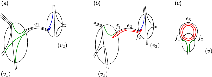
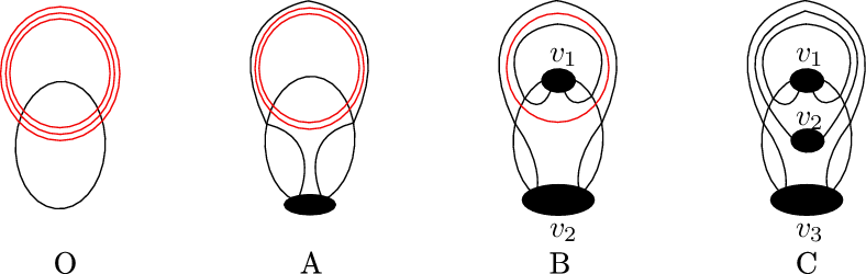
We use, for short, “inner face” or “outer strand” when there is no confusion about the edge they refer to. See Figure 17A, B and C for an illustration in the rank 3 situation. In that figure, A describes a 0–inner edge
 $e_1$
, B a 1–inner edge
 $e_2$
, and C a 2–inner edge
 $e_3$
. The inner faces are highlighted in red therein, and outer strands are the strands of
 $e_i$
,
 $i=1,2,3$
, forming paths with chords highlighted in green and blue.
Some rank 3 p–inner edges: 0–inner
 $e_1$
(A), 1–inner
 $e_2$
(B) and 2–inner
 $e_3$
(C) edges.

The notion of stranded edge contraction can be defined at this point. In contracting an edge e, we look at the subgraph
 $s \cup c$
of associated with e in the larger graph consisting of all strands meeting all chords;
 $s \cup c$
consists of paths and cycles. We replace each cycle by a trivial circle, and each path by a new chord joining its endpoints. This operation does not affect the face structure, except that some (inner) faces may be deleted in the former component containing e. However, the total number of closed and open faces remains constant: to each inner face of e, we associate a trivial circle which then introduces back another closed face in the HESG.
Definition 4.7 (Stranded edge contractions). Let
 $ \mathscr{G} _{\mathfrak{f}^0}$
be a rank D HESG and e be a rank d stranded edge with
 $s \cup c$
the subgraph associated with e in the larger graph consisting of all strands meeting all chords (in the previous notation). Let
 $p\le d$
be a positive integer.
If e is a p–inner edge,
 $ \mathscr{G} _{\mathfrak{f}^0}/e$
is the result of contracting e in
 $ \mathscr{G} _{\mathfrak{f}^0}$
, that is defined from
 $ \mathscr{G} _{\mathfrak{f}^0}$
by replacing e and its end vertices
 $v_{1}$
and
 $v_2$
(or its end vertex v, if e is a loop, respectively) by p trivial circles and a new stranded vertex v
′. The new vertex v
′ possesses all pre-edges except those connected to e and all sHEs as they appear on
 $v_{1}$
and
 $v_{2}$
(respectively, on v), keeping all chords of
 $v_{1}$
and
 $v_{2}$
(respectively, of v) except those involved in the cycles of
 $s \cup c$
, and replacing each open path of
 $s\cup c$
by a new chord joining its ends. If the vertex v
′ is disconnected, then we split it.
If there is no outer strands left after removing the p inner faces of e, then there is no vertex v ′.
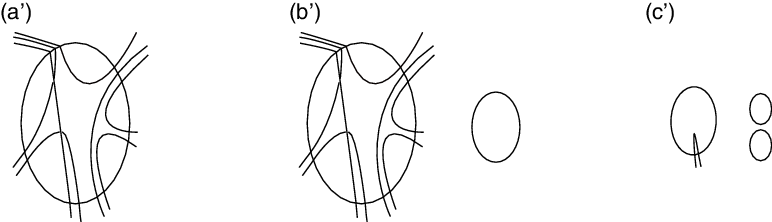
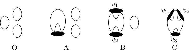
Some examples of rank 3 stranded edge contraction are given in Figure 18A and B, and an example of a rank 3 loop contraction is given in Figure 18C.
Graphs A, B and C obtained after stranded edge contraction of A, B and C of Figure 17, respectively.

A convenient way, though not necessary, to illustrate this type of contraction is to use a cyclic order for
 $v_1$
and
 $v_2$
contract the stranded edge e incident to these vertices and finally draw the final vertex respecting the cyclic order of the pre-edges on
 $v_{1}$
and
 $v_2$
. This choice leads to the representation given in Figure 18.
One may directly check that contracting a non loop in a ribbon graph can be seen as a rank 2 stranded edge contraction. One may also check that a trivial loop contraction for a ribbon graph coincides with the notion of contraction of a loop in the sense of Definition 4.7, when the ribbon graph is viewed as a rank 2 stranded graph. Indeed, in a ribbon graph, a trivial positive loop can be a 0–, 1– or 2–inner loop. A trivial negative loop can be a 1– or 0–inner loop. Contracting these trivial loops in a ribbon graph is equivalent of what is described in Definition 4.7. Discussing loops, we only focus on trivial ones in the following.
The following proposition is straightforward.
Proposition 4.8. Let
 $ \mathscr{G} _{\mathfrak{f}^0}$
be a rank D HESG and e be one of its stranded edge. Then
 $ \mathscr{G} _{\mathfrak{f}^0}/e$
obtained by contraction of e is a rank D′ HESG, with
 $D'\le D$
.
At this point, one may wonder if the additional circles obtained after stranded edge contraction are not inessential features of the HESGs. In fact, they are very useful for the preservation of number of faces during the edge contraction of the stranded graph, in analogy with the case of ribbon graphs. In another context related to the topology associated with the stranded graphs, another type of contraction (without trivial circles involved) can be defined on stranded graphs, see for instance, in [Reference Ben Geloun and Rivasseau7].
Coloured tensor graphs. Apart from the stranded structure, the second important feature that we need is the colouring.
Definition 4.9 (Coloured tensor graph [Reference Gurau17, Reference Gurau and Ryan21]). A rank
 $D\geq 1$
properly coloured tensor graph
 $ \mathscr{G} $
is a rank D tensor graph such that the underlying graph is bipartite and the stranded edges of
 $ \mathscr{G} $
are coloured with
 $D+1$
colours such that no two stranded edges that meet at a stranded vertex have the same colour. The colouring of stranded edges determines the colouring of pre-edges that they meet. The chord colouring is the following: in each stranded vertex, each vertex point has an ordered pair of colours (i, j): i is the colour of the pre-edge it is in, and j is the colour of the pre-edge containing the other end of its chord. (So for each i, j with
 $j \neq i$
there is one point with colour (i, j)). The unordered pair
 $\{i,j\}$
determined by the colouring of the end points of some chord yields the chord colouring. In a stranded edge of colour i, the end points of each strand have the same colour pair (i, j); the unordered pair
 $\{i,j\}$
yields the strand colouring.
The colour restriction introduced in Definition 4.9 allows us to control the type of graphs generated by gluings of stranded vertices and edges. Later, the colouring
 $\{i,j\}$
of strands or chords will be called bi-colouring and we will work with an unordered pair (ij), called colour pair, for strands or chords. Observe that strands and chords that meet have necessarily the same colour pair. For simplicity, we will consider that a coloured tensor graph does not have trivial circles from the beginning. The general case should not be hard to recover with a given assignment of bi-colouring (a prescription by default) of the closed faces of these trivial vertices.
We denote a rank D coloured tensor graph by
 $ \mathscr{G} (\mathcal{V},\mathcal{E})$
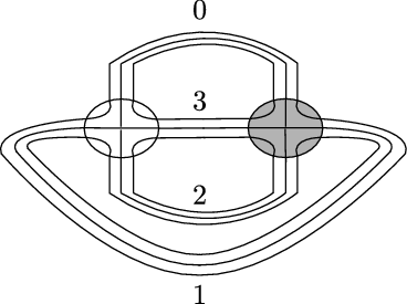
as usual. As an illustration, a rank 3 coloured tensor graph is pictured in Figure 19. Each vertex (with vertex graph
 $K_{4}$
) is the dual of a tetrahedron and an edge represents a triangle endowed with a colour
 $i \in \{0,1,2,3\}$
. The (underlying) graph is also bipartite (white and shaded vertices).
A rank 3 coloured tensor graph.

It turns out that, in any rank, the stranded structure of a coloured tensor graph
 $ \mathscr{G} $
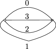
can be captured at the level of its underlying bipartite coloured graph. For instance, the graph of Figure 19 can be also drawn in the collapsed form of Figure 20.
Underlying graph of the graph of Figure 19.

It is worth highlighting that one representation of the graph unambiguously determines the other. This is not the case for a generic underlying graph of a stranded or tensor graph without colours. In order to render this expansion explicit in the coloured case, one must use the bi-colouring of chords and strands. This is the way to proceed: consider a
 $ D+1\geq 2$
edge properly coloured graph G, then replace each vertex by a rank D stranded vertex with coordination
 $D+1$
, with vertex graph
 $K_{{D+1}}$
, and pre-edges with fixed cardinality D. Now replace each coloured edge in G by a rank
 $ D+1$
coloured edge with the same colour and respecting the same incidence relation as in G and form
 $ \mathscr{G} $
a rank D tensor graph. Assign a colour to each pre-edge according to the colouring of the edges incident to these. A bi-colouring for chords and strands can be deduced from that point. This is the rank D coloured tensor graph.
There are certainly more data worthwhile to be discussed in such a coloured graph.
Definition 4.10 (bubbles [Reference Gurau17]). Let
 $ \mathscr{G} $
be a rank D coloured tensor graph.
-
• A 0-bubble is a vertex of
$ \mathscr{G} $
. -
• A 1-bubble is an edge of
$ \mathscr{G} $
. -
• For all
$p \geq 2$
, a p-bubble of
$ \mathscr{G} $
with colours
$i_1 < i_2 < \dots<i_p $
,
$p\leq D$
, and
$i_k\in \{0, \dots, D\}$
is a connected rank
$p-1$
coloured tensor graph the underlying graph of which is a maximal connected subgraph of the underlying graph of
$ \mathscr{G} $
made of edges of colours
$\{i_1, \dots, i_p\}$
.







For
 $p \geq 2$
, a p-bubble can be mapped to a rank
 $p-1$
coloured tensor graph because we can associate to each p coloured graph a rank
 $p-1$
coloured tensor graph according to the procedure explained above.
To obtain the set of p-bubbles is actually easy in a coloured tensor graph
 $ \mathscr{G} $
. Consider the underlying graph of
 $ \mathscr{G} $
. Take a subset C of cardinality p of the set of colours
 $\{0, 1, \dots, D\}$
, delete all edges of colours
 $\{0, 1, \dots, D\} {\setminus} C$
in the underlying graph. Each connnected component of the resulting graph is a p-regular edge coloured graph that determines uniquely a rank
 $p-1$
coloured tensor graph, a p-bubble. We can alternatively perform the deletion at the level of the stranded graph: delete all stranded edges of colour
 $\{0, 1, \dots, D\} {\setminus} C$
, all vertex points, and the chords incident to those, if their colour pair (i,j) involves i or j in
 $\{0, 1, \dots, D\} {\setminus} C$
. Each remaining connected component is a rank
 $p-1$
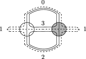
coloured tensor graph that defines a p-bubble.
Restricting to rank
 $D=3$
coloured tensor graphs, there are two types of p-bubbles that we shall study in the following: 2-bubbles coincide with the faces (Definition 4.5) of the coloured tensor graph. Thus, there are alternative ways to observe faces of a coloured tensor graph. Faces can be read from the underlying coloured graph as cycles with alternating (edge) colours. On the other hand, faces are cycles made with chords and strands with a given colour pair (see the face
 $f_{01}$
(in red) in Figure 21). The alternating colours are precisely the colour pair of the strands and chords (in the sense of Definition 4.9) forming the face. They are also rank 1 coloured tensor graphs. 3-bubbles (or simply bubbles in
 $D=3$
) are in one-to-one correspondence with maximal connected components of the underlying graph which have three colours (see Figure 21). These are rank 2 coloured tensor graphs and also coloured ribbon graphs with 3-valent vertices.
The face
 $f_{01}$
(in red) and bubbles of the graph of Figure 19.

As mentioned earlier in this section, a 3-bubble, which is a rank 2 tensor graph, can be seen as a ribbon graph. In
 $D=3$
, the vertices of a bubble are 3-valent vertices obtained by decomposing the vertex of the graph in the way of Figure 21. The edges of a 3-bubble are coloured ribbon edges generated by the decomposition of the coloured stranded edges of the rank D coloured graph. Like ordinary ribbon graphs, 3-bubbles have faces as well. These faces are endowed with a pair of colours like the faces of the initial graph. Thus, a bubble is simply a rank 2 coloured tensor graph lying inside the rank 3 coloured tensor graph. The set of 3-bubbles is denoted by
 $\mathcal{B}_3$
and
 $|\mathcal{B}_3| = B_3$
. The index 3 is omitted when discussing
 $D=3$
.
Rank
D
half-edged coloured tensor graphs. Rank D sHEs can be considered as well on rank D coloured tensor graphs, provided these sHEs possess a colour and their gluing respects the graph colouring at each vertex. For any rank D coloured tensor graph with sHEs, we demand that to each stranded edge and sHE, one assigns a colour
 $i \in \{0,1,\dots,D\}$
such that no two stranded edges or sHEs meeting at a vertex share the same colour.
The cut of a stranded edge can be understood in the same sense of Definition 4.4 for coloured tensor graphs. After cutting a coloured stranded edge, the resulting sHEs possess the same colour of that edge.
Definition 4.11 (Half-edged coloured tensor graph (HEcTG)). A rank D HEcTG is a rank D half-edged tensor graph such that its underlying graph is a bipartite HEG, its stranded edges and sHEs are coloured with
 $D+1$
colours such that no two stranded edges or half-edges meeting at a vertex have the same colour. The colouring of pre-edges, vertex points, and chords of stranded vertices, and the colouring of strands of stranded edges and sHEs are described by Definition 4.9.
An example of a rank
 $D=3$
HEcTG is given on the left in Figure 22 (most left, edges and sHEs are coloured). Spanning c-subgraphs of a HEcTG follow from the similar notion for HESG and from Definition 2.5. The only point to be added is the colouring.
A rank 3 HEcTG and its bubbles;
 $f_{01}$
(highlighted in red) is an open face;
 $\mathbf{b}_{012}$
,
 $\mathbf{b}_{013}$
and
 $\mathbf{b}_{123}$
are open bubbles and
 $\mathbf{b}_{023}$
is closed.

The following is straightforward:
Proposition 4.12. Spanning c-subgraphs of a rank D HEcTG are rank D HEcTG.
Let us investigate some properties of a HEcTG
 $ \mathscr{G} _{\mathfrak{f}^0}$
. The notion of bridge is standard. By definition of a proper edge colouring, HEcTGs cannot contain loops.
As in the case of HESGs, by introducing sHEs on coloured tensor graphs, we distinguish two types of faces. Using Definition 4.5, faces can be open or closed connected components if they pass through external points of sHEs or not (let us recall that these are also cycles and paths in the abstract graph formed by all strands and chords of the underlying HESG). An open face with colour pair (01) is highlighted in red in Figure 22. The sets of closed and open faces are denoted by
 $\mathcal{F}_{{\textrm{int}}}$
and
 $\mathcal{F}_{{\textrm{ext}}}$
, respectively. Hence, for a rank D HEcTG, the set
 $\mathcal{F}$
of faces is the disjoint union
 $\mathcal{F}_{{\textrm{int}}} \cup \mathcal{F}_{{\textrm{ext}}}$
.
To define p-bubbles for HEcTG, we simply replace “edge” by “edge or sHE”, and “underlying graph” by “underlying HEG” in Definition 4.10. We say that a p-bubble in some HEcTG
 $ \mathscr{G} _{\mathfrak{f}^0}$
is open if its underlying graph contains half-edges. Hence, a p-bubble is open if it contains open faces, otherwise it is closed. Open and closed bubbles for a rank 3 HEcTG have been illustrated in Figure 22. The sets of closed and open bubbles are denoted by
 $\mathcal{B}_{{\textrm{int}}}$
and
 $\mathcal{B}_{{\textrm{ext}}}$
, respectively.
The following notion will play a crucial role in our following construction upon HEcTG. That notion turns out to be defined at the generic level of HESG.
Definition 4.13 (Boundary of an HESG). The boundary graph
 $ {\partial \mathscr{G}_{ \mathfrak{f}^0 } } ({\mathcal{V}}_{\partial},{\mathcal{E}}_{\partial})$
of a rank D HESG
 $ \mathscr{G} (\mathcal{V},\mathcal{E},\mathfrak{f}^0)$
is a graph with vertex set
 ${\mathcal{V}}_{\partial}$
in one-to-one correspondence with
 $\mathfrak{f}^0$
, with edge set
 ${\mathcal{E}}_{\partial}$
in one-to-one correspondence with
 $ \mathcal{F}_{{\textrm{ext}}}$
. Consider an edge
 $e \in {\mathcal{E}}_{\partial}$
, its corresponding open face
 $f_e\in\mathcal{F}_{{\textrm{ext}}}$
, a vertex
 $v \in {\mathcal{V}}_{\partial}$
, and its corresponding sHE
 $h_v$
. Then, e is incident to v if and only if
 $f_e$
has one end point in
 $h_v$
. The boundary graph of a rank D HESG with
 $\mathfrak{f}^0=\emptyset$
is empty.
There is a procedure for drawing the boundary graph of a rank D HESG described by Gurau as pinching in [Reference Gurau20]. Insert a vertex at each sHE and make them incident to the strands of the sHE (they become incident to the open faces). In the case of a rank D half-edged tensor graph, the vertices of the boundary graph must be D-regular vertices. In doing so for the rank 3 HEcTG of Figure 22 (most left), we associate its boundary depicted in Figure 23. In fact, the colouring of a HEcTG entails a new colouring on its boundary graph. Both types of colourings will allow us to enumerate the different constituents (or to find bounds on their number) of these generalized graphs.
Boundary graph (in dashed lines) of the graph of Figure 22.

Definition 4.14 (Ve-coloured graphs). A
 $(D+1)$
ve-coloured graph is a graph with a vertex colouring with colours from
 $\{0,\dots,D\}$
and a proper edge colouring such that each edge is assigned an unordered pair (ab) of colours, a,b in
 $\{0,\dots,D\}$
,
 $a\neq b$
, and such that the end vertices of an edge with colour (ab) must have colour a or b. The two ends may or may not have distinct colours.
Some 4 ve-coloured graphs are drawn in Figure 24.
Examples of 4 ve-coloured graphs.

One notices that a
 $(D+1)$
ve-coloured graph is a
 $D(D+1)/2$
edge coloured graph, with edge colours chosen in pairs ab,
 $a<b$
, in
 $\{01,02, \dots, 0D, 12,\dots, (D-1)D\}$
. Because of the proper edge colouring, ve-coloured graphs have no loops.
Definition 4.15 (Ve-coloured tensor graph). A rank
 $D\geq 1$
ve-coloured tensor graph
 $ \mathscr{G} $
is a rank D tensor graph in which
-
1. every stranded vertex has a colour from
$\{0, 1, \cdots , D+1\}$
; within a stranded vertex of colour i, the
$D+1$
pre-edges have each a distinct colour pair ij, where
$0 \leq j \leq D+1$
,
$j \ne i$
(vertex colouring); -
2. every stranded edge has a colour pair i j, where
$0 \leq i, j \leq D+1$
are distinct, such that no two stranded edges that meet at a stranded vertex have the same colour pair (proper edge colouring). -
3. If a stranded vertex v is an end of a stranded edge e of colour pair i j, then v must have colour i or colour j. The colourings of the pre-edges and stranded edges are consistent in the natural sense: if a pre-edge and a stranded edge meet, they must have the same colour pair.
-
4. Every strand and every chord has a colour triple i j k, where
$0 \leq i, j, k \leq D$
are pairwise distinct, with the following properties:-
i. within a stranded vertex v of colour i, a chord that is incident to two vertex points of two pre-edges of distinct colour pair ij and ik has colour ijk,
$k \notin \{i, j\}$
; -
ii. within a stranded edge e with colour i j, there are exactly D strands, with D colour triples i j k,
$k \notin \{i, j\}$
; -
iii. if a strand and a chord meet at a vertex point they must have the same colour triple ijk.
-


Note that a ve-coloured tensor graph is not a coloured tensor graph. For instance, it may be not bipartite.
Proposition 4.16 (Underlying graph of a ve-coloured tensor graph). The underlying graph of a rank D ve-coloured tensor graph is
 $(D+2)$
ve-coloured and
 $D+1$
regular.
Proof. The proof is fairly straightforward. Let
 $ \mathscr{G} $
be a rank D ve-coloured tensor graph and G be its corresponding underlying graph. The graph G is
 $D+1$
regular just like
 $ \mathscr{G} $
is. G inherits from
 $ \mathscr{G} $
the vertex colouring with colours from
 $\{0, \cdots, D+1\}$
. Since each edge e of
 $\mathcal{G}$
is in one-to-one correspondence with a stranded edge e
′ of
 $ \mathscr{G} $
, we assign to e the colour pair i j of e
′ where
 $0 \leq i, j \leq D+1$
are distinct. This also implies that no two edges in G that meet at a vertex have the same colour pair. The last condition stating that the end vertices of an edge e of G with colour pair ij must have colour i or j is also fulfilled: the third point in Definition 4.15 holds for
 $ \mathscr{G} $
and this reflects on G.
Proposition 4.17. A
 $(D+2)$
ve-coloured graph which is
 $(D+1)$
regular uniquely determines a rank D ve-coloured tensor graph of which it is the underlying graph.
Proof. Consider G(V,E) a
 $(D+2)$
ve-coloured graph, with colours
 $\{0,1,\dots, D+1\}$
, that is
 $(D+1)$
regular. To each vertex v of V, we assign a rank D stranded vertex v
′ with coordination
 $D+1$
with vertex graph
 $K_{{D+1}}$
, and pre-edges with fixed cardinality D. The vertex colouring is carried along, from the vertices of V to the stranded vertices. In a given stranded vertex v
′ of colour i, all
 $D+1$
pre-edges can be given a distinct colour pair ij in a way compatible with the first point of Definition 4.15. This fills the point (1). The point 4(i) of this definition can be also implemented without ambiguity given the pre-edge bi-colouring. Now replace every edge e in G of colour pair ij by a rank D coloured edge e
′ with the same colour pair ij. We keep the incidence relation between all corresponding stranded edges and vertices. Hence the proper edge colouring is carried along. This fulfills condition (2). Note that we have not yet specified the chord-strand connection. Let us address (3). Since e of colour pair ij in G is incident to vertices of colour i or j, the same should apply to the corresponding stranded edge e
′: it is incident to stranded vertices of colour i or j. A stranded vertex v
′ of colour i has exactly
 $D+1$
pre-edges with distinct colour pair ij, on which must end a stranded edge of the same pair ij. There is no ambiguity and therefore (3) holds. It only remains to specify the connection between strands and chords at the level of a single stranded edge and vertex connection. Take a rank D stranded edge e
′ with colour pair ij incident to a stranded vertex v
′ of colour i. Construct the colouring of the D strands of e
′ so that 4(ii) is obeyed. We immediately see that there is a one-to-one correspondence between the colour triples ijk of the strands of e
′ and the colour triples ijk of the chords at the pre-edge of v
′ incident to e
′. There is a single choice for the connection strand-chords so that 4(iii) holds. Finally, it is obvious that the underlying graph of the constructed stranded graph is our initial graph G.
Proposition 4.18. (Ve-colouring of
 $ {\partial \mathscr{G}_{ \mathfrak{f}^0 } } $
). The boundary graph
 $ {\partial \mathscr{G}_{ \mathfrak{f}^0 } } ({\mathcal{V}}_{\partial},{\mathcal{E}}_{\partial})$
of a rank D HEcTG
 $ \mathscr{G} (\mathcal{V},\mathcal{E},\mathfrak{f}^0)$
is
 $(D+1)$
ve-coloured and determines in a unique way a rank
 $(D-1)$
ve-coloured tensor graph.
Proof. The vertex colouring of
 $ {\partial \mathscr{G}_{ \mathfrak{f}^0 } } $
is inherited from the colouring of the sHEs of
 $ \mathscr{G} _{\mathfrak{f}^0}$
, that is to each vertex of
 $ {\partial \mathscr{G}_{ \mathfrak{f}^0 } } $
, one assigns the same colour of its corresponding sHE. The edge bi-colouring in
 $ {\partial \mathscr{G}_{ \mathfrak{f}^0 } } $
coincides with the open face bi-colouring. At a sHE, the colour pairs of all open faces never coincide. This makes the graph
 $ {\partial \mathscr{G}_{ \mathfrak{f}^0 } } $
 $(D+1)$
ve-coloured. Furthermore the graph
 $ {\partial \mathscr{G}_{ \mathfrak{f}^0 } } $
is D-regular as
 $ \mathscr{G} _{\mathfrak{f}^0}$
is of rank D and so are its sHEs. The existence of a unique
 $(D-1)$
ve-coloured tensor graph associated with
 $ {\partial \mathscr{G}_{ \mathfrak{f}^0 } } $
follows from Proposition 4.17.
With Proposition 4.18, we can identify the boundary graph
 $ {\partial \mathscr{G}_{ \mathfrak{f}^0 } } $
with the rank
 $D-1$
ve-coloured stranded graph associated with it.
A boundary graph does not have sHEs hence all of its faces are closed. We take an example in rank
 $D=3$
, see Figure 25. Each vertex of
 $ {\partial \mathscr{G}_{ \mathfrak{f}^0 } } $
is coloured and is 3 valent. Each edge of
 $ {\partial \mathscr{G}_{ \mathfrak{f}^0 } } $
is mapped to a bi-coloured ribbon, and each face is closed.
Rank 2 ve-coloured stranded structure of the boundary graph of Figure 22.

Remark 4.19 Let us discuss a feature in rank
 $D=3$
that will be important for the next computations. Consider a HEcTG
 $ \mathscr{G} _{\mathfrak{f}^0}$
, its boundary graph
 $ {\partial \mathscr{G}_{ \mathfrak{f}^0 } } $
, its set of open bubbles, each of them viewed as a HERG (rank 2), and the set of their boundary graph. As a rank 1 graph, the boundary graph of any open bubble is only made of cycles that are still called faces. A face of
 $ {\partial \mathscr{G}_{ \mathfrak{f}^0 } } $
is a cycle made of strands and chords coming from open faces of
 $ \mathscr{G} _{\mathfrak{f}^0}$
. These strands and chords, respectively, necessarily belong to stranded edges and vertices, respectively, of open bubbles in
 $ \mathscr{G} _{\mathfrak{f}^0}$
(remember that we decompose
 $ \mathscr{G} _{\mathfrak{f}^0}$
in maximal connected 3 coloured graphs, the bubbles). By taking the boundary graph of such open bubbles, we produce cycles which are in one-to-one correspondence with the set of (closed) faces of
 $ {\partial \mathscr{G}_{ \mathfrak{f}^0 } } $
.
As an illustration of the above remark, consider the HEcTG
 $ \mathscr{G} _{\mathfrak{f}^0}$
given in Figure 22, with boundary
 $ {\partial \mathscr{G}_{ \mathfrak{f}^0 } } $
drawn in Figure 23. Let us pick the face
 $f_{102}$
of
 $ {\partial \mathscr{G}_{ \mathfrak{f}^0 } } $
that is a face (obviously closed) made of the strands with colour pairs (12) and (10), and chords of the vertex of colour 1. Consider the unique open bubble
 $\mathbf{b}_{012}$
of
 $ \mathscr{G} _{\mathfrak{f}^0}$
as a HERG. The open faces
 $f^{\prime}_{10}$
and
 $f^{\prime}_{12}$
of
 $\mathbf{b}_{012}$
will generate a cycle in its boundary graph
 $\partial \mathbf{b}_{012}$
that is corresponding to
 $f_{102}$
. Furthermore, such a closed face cannot belong to another bubble by colour exclusion and the fact that each strand of a given stranded edge is exactly used twice to make two stranded edges of two different bubbles of
 $ \mathscr{G} _{\mathfrak{f}^0}$
(for instance the strand of colour (01) making
 $f^{\prime}_{01}$
is used once in
 $\mathbf{b}_{012}$
and once in
 $\mathbf{b}_{013}$
). We illustrate this fact once again in a slightly more involved situation given by Figure 26.
A HEcTG, its boundary, and its expansion as a ribbon graph. The face
 $f_{012}$
is made from the open faces
 $f_{01}$
and
 $f_{12}$
.
 $f_{01}$
appears in 2 open bubbles,
 $\mathbf{b}_{012}$
and
 $\mathbf{b}_{013}$
.
 $f_{012}$
corresponds to a cycle in
 $\partial\mathbf{b}_{012}$
.

4.2. W-coloured stranded graphs
It has been discussed earlier that the contraction of a stranded edge in a coloured tensor graph yields another type of graph for which neither proper edge colouring, nor the tensor axioms (Definition 4.2) apply. In order to circumvent such an odd feature of tensor graphs and thereby find polynomial invariants on these structure, some proposals have been made to redefine the notion of contraction of an edge or redefine subgraphs for which the contraction applies [Reference Gurau20, Reference Tanasa28]. In the following, we use a different scheme.
Using Definition 4.7, we can now contract any rank D edge provided the fact that we are working in the extended framework of stranded graphs. This definition therefore applies to a HEcTG. From now on, edge contraction means always stranded edge contraction in the sense Definition 4.7.
Definition 4.20 (Rank w-coloured graph). A rank D weakly coloured or w-coloured graph is a rank D HESG obtained by zero or more, successive stranded edge contractions of some rank D HEcTG.
Few remarks must be made at this point. Any HEcTG is a w-coloured graph of the same rank when no stranded edge contractions have been performed. For any coloured graph, any edge contraction breaks the proper edge colouring (see an example, a rank
 $D=3$
edge contraction in a HEcTG in Figure 27). However, in rank D, there is a colour structure on
 $ \mathscr{G} _{\mathfrak{f}^0}/e$
defined in a weaker sense. Such a weak colouring, that we plan to investigate, is based on the property that any stranded edge contraction preserves faces, the colouring of vertex points, and the bi-colouring of faces.
Contraction of an edge in a rank 3 HEcTG.

Finally, several HEcTGs may generate the same w-coloured graph by edge contractions.
Lemma 4.21 (Stability of the boundary graph under stranded edged contraction).
-
• Contracting a stranded edge in a rank D HESG
$ \mathscr{G} _{\mathfrak{f}^0}$
does not change its boundary graph.
-
• The contraction in arbitrary order of all stranded edges of
$ \mathscr{G} _{\mathfrak{f}^0}$
yields a HESG
$ \mathscr{G} ^0_{\mathfrak{f}^0}$
determined by the boundary graph
$ {\partial \mathscr{G}_{ \mathfrak{f}^0 } } $
of
$ \mathscr{G} _{\mathfrak{f}^0}$
up to additional trivial circles.


Proof. Consider a HESG
 $ \mathscr{G} _{\mathfrak{f}^0}$
with boundary graph
 $ {\partial \mathscr{G}_{ \mathfrak{f}^0 } } $
. After contracting a stranded edge in
 $ \mathscr{G} _{\mathfrak{f}^0}$
, all sHEs remain untouched and all open faces might shrink by loosing strands and chords but the resulting set of open faces is in one-to-one correspondence with the former. No open face can be created by such operations (we remove all present inner faces and all remaining faces get shorter but are never cut). Hence, for the resulting stranded graph
 $ \mathscr{G} _{\mathfrak{f}^0}/e$
, one has
 $\partial ( \mathscr{G} _{\mathfrak{f}^0}/e)= {\partial \mathscr{G}_{ \mathfrak{f}^0 } } $
. By iteration, contracting all edges of
 $ \mathscr{G} _{\mathfrak{f}^0}$
in arbitrary order, the resulting graph
 $ \mathscr{G} _{\mathfrak{f}^0}^0$
should contain
 $ {\partial \mathscr{G}_{ \mathfrak{f}^0 } } $
as its boundary. Contracting all edges of
 $ \mathscr{G} _{\mathfrak{f}^0}$
, one obtains a single stranded vertex graph per connected component plus trivial circles. Then, necessarily,
 $ \mathscr{G} _{\mathfrak{f}^0}^0$
is nothing but a graph made only with stranded vertices (without edges) and sHEs attached to these. Then
 $ \mathscr{G} ^0_{\mathfrak{f}^0}$
is therefore defined by
 $\partial \mathscr{G} ^0_{\mathfrak{f}^0}= {\partial \mathscr{G}_{ \mathfrak{f}^0 } } $
up to trivial circles.
First, we observe that the previous lemma restricts to half-edged tensor graphs without colours. Second, consider
 $ \mathscr{G} _{\mathfrak{f}^0}$
a connected HEcTG with a nonempty set of sHEs,
 $\mathfrak{f}^0\neq \emptyset$
. After a full contraction of all edges of
 $ \mathscr{G} _{\mathfrak{f}^0}$
, Lemma 4.21 tells us that the end result
 $ \mathscr{G} _{\mathfrak{f}^0}^0$
is totally encoded in the boundary graph
 $ {\partial \mathscr{G}_{ \mathfrak{f}^0 } } $
up to some circles. If
 $\mathfrak{f}^0 = \emptyset$
, then there is no boundary in
 $ \mathscr{G} _{\emptyset}$
, and
 $ \mathscr{G} ^0_{\emptyset}$
consists of trivial circles, if non empty.
Our next goal is to investigate the properties that the contraction and cut operations have on w-coloured graphs.
Lemma 4.22. Let e be an ordinary stranded edge or a bridge of a rank 3 w-coloured graph. Contracting e yields a stranded vertex which is connected.
Proof. An argument on the parity of the number of pre-edge points of a given colour pair and the fact that two strands of a coloured stranded edge in a w-coloured graph cannot have the same colour pair achieve this proof. The detail of the proof follows.
Without loss of generality, let us assume that e is of a given colour, say 0. Each of its strands is of colour pair (0i),
 $i=1,2,3$
. Let us concentrate on a single stranded vertex v, of vertex graph v′, where e is incident at a pre-edge
 $f_e$
. If the contraction of e disconnects the resulting stranded pre-vertex, there are at least two non-empty and distinct sets of pre-edges in v, namely
 $v_1$
and
 $v_2$
, that form two disctinct subgraphs
 $s_1$
and
 $s_2$
of v
′, respectively, that are connected only via the vertex corresponding to
 $f_e$
in v
′. In other words, there are no edge connections between
 $s_1$
and
 $s_2$
. Note also that
 $f_e$
does not belong neither to
 $v_1$
nor to
 $v_2$
.
There are three strands in e. The three of them cannot join the same subset of pre-edges, otherwise it would mean that v was initially disconnected (if
 $v_1$
and
 $v_2$
are non empty) or v was made only with two pre-edges which also trivializes the proof. Thus, at most 2 strands of e could join one subset of pre-edges and the last should connect the other one.
Consider the strand of colour pair (01) in e. This strand is incident to a chord (at a pre-edge point) incident itself to another pre-edge called f. The pre-edge f is necessarily of colour 0 or 1. Without loss of generality, let us assume that f is the unique pre-edge connected to
 $f_e$
and that also belongs to the set of pre-edges
 $v_1$
. Because we can exchange the role played by the colours 0 and 1, we can fix the colour of f to be 1. Denote
 $N_i$
the number of pre-edges of colour i in
 $v_1$
.
-
− There are
$N_i$
pre-edge points of colour pair (i,j) in
$v_1$
, for fixed
$i=0,2,3$
, and
$j\in \{0,1,2,3\}$
but
$j\ne i$
. -
− There are
$N_1$
pre-edge points of colour pair (1,j) in
$v_1$
, for fixed
$j=2,3$
. -
− There are
$N_1-1$
pre-edge points of colour pair (1,0) in
$v_1$
.


The chords in
 $v_1$
should connect all these pre-edges points. Denoting
 $k^{ij}$
the number of chords of colour (ij) in
 $v_1$
, we have
 \begin{align}
N_0 + N_1 - 1 = 2k^{01}\nonumber\\[4pt]
N_0 + N_2 =2k^{02}\nonumber\\[4pt]
N_1 + N_2 = 2k^{12}\end{align}
which entails an inconsistent equation:
 $2N_0 + 2(k^{02} - k^{12}) -1 = 2k^{01}$
.
The above lemma should admit an extension to any rank D by partitioning D and analysing the connection of the strands of e and the chords of the vertices that it meets. We do not need however such a stronger result for the following.
In contrast, the contraction of a loop may disconnect the vertex. In any case, since loop graphs are terminal forms, a special treatment is required for them.
The whole above construction maintains the consistency of the definition of p-bubbles. In a w-coloured graph, stranded vertices are still 0-bubbles (connected objects with 0 colour), stranded edges are 1-bubbles (connected objects with 1 colour), (closed and open) faces are bi-coloured maximal connected objects, (closed and open) 3-bubbles are maximal connected objects with 3 colours. It should be however noticed that :
-
1. closed faces of the trivial circle vertices naturally inherit of the bi-colouring of the faces they are coming from;
-
2. 3-bubbles are no longer built uniquely with three valent vertices. They can be made with vertices with lower or greater valence as illustrated in Figure 28. In any case, Definition 4.10 is still valid and we shall focus on this.
Figure 28.Two bubbles graphs
$\mathbf{b}_1$
and
$\mathbf{b}_2$
of
$ \mathscr{G} _{1;\mathfrak{f}^0}$
and
$ \mathscr{G} _{2;\mathfrak{f}^0}$
, respectively:
$\mathbf{b}_1$
has a vertex with valence 2 and
$\mathbf{b}_2$
a vertex with valence 4.


From now on, general discussions are always valid at fixed rank D, thus we shall omit to mention it. Focusing on operations on w-coloured graphs, key notions pertain again to the cut/contraction rules.
Lemma 4.23. Let
 $ \mathscr{G}_{ \mathfrak{f}^0} $
be a rank D w-coloured graph and e one of its stranded edges.
 $ \mathscr{G}_{ \mathfrak{f}^0} \vee e$
the cut graph along e, is a rank D w-coloured graph.
 $ \mathscr{G}_{ \mathfrak{f}^0} /e$
, called the contraction of
 $ \mathscr{G}_{ \mathfrak{f}^0} $
along e, is a rank D w-coloured graph.
Proof. Let
 $ \mathscr{G}_{ \mathfrak{f}^0} $
be the result of a contraction of some HEcTG
 $ \mathscr{G}_{ \text{color}; \mathfrak{f}^0} $
. We want to show that both
 $ \mathscr{G}_{ \mathfrak{f}^0} \vee e$
and
 $ \mathscr{G}_{ \mathfrak{f}^0} /e$
come from edge contractions of some HEcTGs. The HEcTG
 $ \mathscr{G}_{ \text{color}; \mathfrak{f}^0} \vee e$
obviously contracts to give
 $ \mathscr{G}_{ \mathfrak{f}^0} \vee e$
. There exists a HEcTG
 $ \mathscr{G}_{ \text{color}; \mathfrak{f}^0} ^0$
contracting to
 $ \mathscr{G}_{ \mathfrak{f}^0} /e$
. This is nothing but
 $ \mathscr{G}_{ \text{color}; \mathfrak{f}^0} $
on which, before performing all contractions yielding
 $ \mathscr{G}_{ \mathfrak{f}^0} $
, one performs the contraction along e.
To define spanning c-subgraphs of a w-coloured graph, we follow the same procedure as the one dealing with HESGs.
Rank 3 w-coloured graph. We henceforth restrict the rank of stranded graphs to
 $D=3$
, and aim at studying an invariant polynomial satisfying a contraction/cut relation, and generalizing the Tutte and BR polynomials for these new graphs. The extension for any D should require more work on the subsequent analysis. From now rank 3 w-coloured graphs are called more simply w-coloured graphs.
Mostly, we have studied non-loop edges so far and their main properties under contraction and cut can be guessed in any rank. Loops are more subtle and their behaviour under contraction is much more involved. Restricting to rank 3 simplifies the analysis.
The contraction of a loop edge may disconnect a stranded vertex and the resulting HESG. Several cases may be discussed according to the number of connected components into which the vertex graph decomposes upon contraction and whether there are stranded edges linking these components.
The contraction of a loop edge e may remove some chords within the stranded vertex v on which e is incident. From this removal may result a disconnection the vertex graph of v. Let us study this in details.
Given a strand s of a stranded edge e incident to stranded vertex v. We call sector of s, the union of the set of chords and set pre-edge points in v that defines a connected component vertex graph on which is incident s, when e is contracted. If a strand contributes to an inner loop, then its sector is empty. Stranded edges and sHEs may be incident to some pre-edges of a given sector. A sector and its incident stranded edges and sHEs will be pictured as a black diagram. Looking at the set of strands of a fixed stranded edge e incident to v, the sectors associated with the strands are called sectors of v. For a rank
 $D=3$
HESG, for a given rank
 $D=3$
stranded edge e incident to v, we have at most three sectors in v.
We now restrict to the case of rank 3 w-coloured graphs. A loop can be at most a 3–inner edge. A 3–inner edge determines by itself a graph, see Figure 29O. If it is a 2–inner loop, then e should be of the form illustrated in Figure 29A. Otherwise, e may be a 1–inner loop (Figure 29B), or a 0–inner (Figure 29C).
p–inner loops: a 3–inner (O) and a 2–inner (A) loop with their unique possible configuration; a 1–inner loop with two potential sectors
 $v_1$
and
 $v_2$
(B), and a 0–inner loop with three potential sectors
 $v_1,v_2$
and
 $v_3$
(C).

For a 2–inner loop e, the outer strand of e should be incident to chords linked to pre-edges meeting sHEs or edges (otherwise e would be a 3–inner edge) : it has a unique sector and we represent the rest of the stranded vertex possibly with edges and sHEs attached, by a black diagram in Figure 29A.
A 1–inner loop e has two outer strands which should be incident to, potentially, two distinct sectors,
 $v_1$
and
 $v_2$
of the vertex, as illustrated in Figure 29B. Any sector,
 $v_1$
or
 $v_2$
, has at least two sHEs or edges because two chords with the same colour pair are incident on their pre-edges.
A 0–inner loop e has potentially three such sectors,
 $v_1,v_2$
and
 $v_3$
. Each sector should contain at least two sHEs or edges.
The notion of trivial loop in HEcTG can be addressed at this point. We call a loop e trivial if it is a 3–inner or a 2–inner loop, or if it is a 1–inner with exactly 2 sectors (upon contraction of e leads to 2 connected component vertex graphs) or 0–inner loop with exactly 3 sectors (upon contraction of e leads to 3 connected component vertex graphs) such that there are no stranded edges linking different sectors.
For a 3–inner loop, the contraction gives three trivial circles, see Figure 30O. The contraction of a trivial 2–inner loop is again straightforward and yields Figure 30A. For a 1–inner loop contraction (see Figure 30B), one gets one additional trivial circle, and has two possible configurations: either the stranded vertex remains connected or it gets disconnected with two (possibly non-trivial) stranded vertices in both situations. Concerning the contraction of a trivial 1–inner loop, it is immediate that the vertex gets disconnected in two non-trivial vertices. For a 0–inner loop contraction (see Figure 30C), we have no additional circles but three types of configurations with up to three disconnected (and possibly non-trivial) stranded vertices. The contraction of a trivial 0–inner loop yields three disconnected and non-trivial stranded vertices.
p–inner loop contractions corresponding to O, A, B and C of Figure 29, respectively.

Lemma 4.24 (Rank 3 trivial loop contraction). Let
 $ \mathscr{G}_{ \mathfrak{f}^0} $
be a w-coloured graph with boundary graph
 $ {\partial \mathscr{G}_{ \mathfrak{f}^0 } } $
, e be a trivial loop of
 $ \mathscr{G}_{ \mathfrak{f}^0} $
,
 $ \mathscr{G}^{\,\prime}_{ \mathfrak{f}^0} = \mathscr{G}_{ \mathfrak{f}^0} /e$
and its boundary graph denoted by
 $ {\partial \mathscr{G}^{\,\prime}_{ \mathfrak{f}^0 } } $
. Let k denote the number of connected components of
 $ \mathscr{G}_{ \mathfrak{f}^0} $
, V its number of stranded vertices, E its number of stranded edges,
 $F_{{\textrm{int}}}$
its number of closed faces,
 $B_{\textrm{int}}$
its number of closed bubbles, and
 $B_{\textrm{ext}}$
its number of open bubbles,
 $C_\partial$
the number of connected components of
 $ {\partial \mathscr{G}_{ \mathfrak{f}^0 } } $
,
 $f=V_\partial$
its number of sHEs,
 $E_\partial=F_{{\textrm{ext}}}$
the number of edges, and
 $F_\partial$
the number of (closed) faces of
 $ {\partial \mathscr{G}_{ \mathfrak{f}^0 } } $
, and let
 $k',V',E',F_{{\textrm{int}}},C^{\prime}_\partial, B^{\prime}_{{\textrm{int}}},B^{\prime}_{\textrm{ext}}, C^{\prime}_\partial,f', E^{\prime}_\partial$
, and
 $F^{\prime}_\partial$
denote the analog numbers for
 $ \mathscr{G}^{\,\prime}_{ \mathfrak{f}^0}$
and
 $ {\partial \mathscr{G}^{\,\prime}_{ \mathfrak{f}^0 } }$
.
If e is a 3–inner loop, then
 \begin{eqnarray}&&k' = k + 2\,, \quad V' = V+2 \,, \quad E' = E-1 \, , \quad F^{\prime}_{{\textrm{int}}} = F_{{\textrm{int}}} \,, \\ &&C^{\prime}_\partial= C_\partial \,, \quad f' = f\,, \quad E^{\prime}_\partial = E_\partial\, ,\quad F^{\prime}_{\partial } = F_{\partial }\,, \\ && B^{\prime}_{\textrm{int}} = B_{{\textrm{int}}} -3\,, \qquad B^{\prime}_{\textrm{ext}} = B_{\textrm{ext}}\,. \end{eqnarray}
If e is a 2–inner loop, then
 \begin{eqnarray}&&k' = k + 2 \,, \quad V' = V+2 \,, \quad E' = E-1 \, , \quad F^{\prime}_{{\textrm{int}}} = F_{{\textrm{int}}} \,, \\ &&C^{\prime}_\partial= C_\partial \,, \quad f' = f\,, \quad E^{\prime}_\partial = E_\partial \,, \quad F^{\prime}_\partial = F_\partial \,, \\ &&B^{\prime}_{\textrm{int}} = B_{{\textrm{int}}} -1\,, \qquad B^{\prime}_{\textrm{ext}} = B_{\textrm{ext}}\,. \end{eqnarray}
If e is a trivial p–inner loop such that
 $p=0,1$
, then
 \begin{eqnarray}&&k' = k + 2 \,, \quad V' = V+2 \,, \quad E' = E-1 \, , \quad F^{\prime}_{{\textrm{int}}} = F_{{\textrm{int}}} \,, \\ &&C^{\prime}_\partial= C_\partial \,, \quad f' = f\,, \quad E^{\prime}_\partial = E_\partial \,, \quad F^{\prime}_\partial = F_\partial \,, \\ &&B^{\prime}_{\textrm{int}} + B^{\prime}_{\textrm{ext}} = B_{{\textrm{int}}} + B_{\textrm{ext}} + \alpha_p \,, \end{eqnarray}
where
 $\alpha_{p} =3-2p$
.
The first situation of a 3–inner loop defines a particular graph without sHEs made of a single vertex with a unique loop. The contraction removes the vertex and the three closed bubbles, and generate three trivial circles. The result (31) follows.
For p–inner loops,
 $p\leq 2$
, there should be other sHEs or edges on the same end vertex. The first lines of (32)–(33) should not cause any difficulty using the definition of the contraction which preserve (open and closed) strands. Let us focus on the variations of the number of bubbles of the graph.
Consider that e is 2–inner. One first should notice that there is a closed bubble formed by the two inner faces of e and that contracting e destroys this bubble. In addition, the other (open or closed) bubbles, which are made of strands of e and containing one of the two inner faces, are simply deformed. They loose one face (the inner) but remain in the contracted graph. The second line of (32) follows.
Let us assume now that e is trivial and 1– or 0–inner, and of colour a. Consider in the initial vertex v, the two or three distinct sectors
 $v_1$
,
 $v_2$
and
 $v_3$
, respectively, determined by the strands of e. We recall that
 $v_1$
,
 $v_2$
, and
 $v_3$
should contain each at least two sHEs or edges. Consider as well the three bubbles labelled by colours
 $(aa_1a_2)$
,
 $(aa_1a_3)$
and
 $(aa_2a_3)$
containing strands of e.
We treat the case of e trivial 1–inner loop, and let us assume that the face
 $(aa_3)$
is the one which is inner, without loss of generality. The edge e decomposes in three ribbon edges each determined by a couple of pairs
 $(aa_i; aa_j)$
,
 $i<j$
, such that the strand
 $(aa_1)$
connects to the sector
 $v_1$
and the strand
 $(aa_2)$
connects to
 $v_2$
. If e is trivial and 1–inner, its contraction yields two connected vertices plus one circle. Consider the bubbles
 $\mathbf{b}_{aa_1a_3}$
and
 $\mathbf{b}_{aa_2a_3}$
(in the whole graph) which are the only ones containing the face
 $(aa_3)$
. Contracting e, the bubbles
 $\mathbf{b}_{aa_1a_3}$
and
 $\mathbf{b}_{aa_2a_3}$
just loose that face and get deformed. They are still present since, in
 $v_1$
and
 $v_2$
, there are still faces that are included in
 $\mathbf{b}_{aa_1a_3}$
and
 $\mathbf{b}_{aa_2a_3}$
. Meanwhile, the last bubble
 $\mathbf{b}_{aa_1a_2}$
splits in two parts: these parts are disjoint bubbles with the same triple of colours since there are no edges in the stranded graph that relate them. These bubbles can be open or closed depending on the nature of
 $\mathbf{b}_{aa_1a_3}$
in
 $v_1$
and
 $v_2$
. Hence,
 $B^{\prime}_{{\textrm{int}}} + B^{\prime}_{\textrm{ext}} = B_{{\textrm{int}}} + B_{\textrm{ext}}+1$
.
Finally, let us discuss the trivial 0–inner loop situation with its three distinct sectors
 $v_1$
,
 $v_2$
and
 $v_3$
. The discussion is somehow similar to the 1–inner case. The contraction of e yields three connected vertices. Using the similar routine explained above, one finds that each of the bubbles
 $\mathbf{b}_{aa_ia_j}$
,
 $i<j$
, gets split into two parts after the contraction. Each of these pairs of parts are not related at all by any stranded edge. Thus each bubble produces two bubbles. The resulting bubbles may be open or closed depending on the nature of
 $\mathbf{b}_{aa_ia_j}$
in each sector. We have
 $B^{\prime}_{{\textrm{int}}} + B^{\prime}_{\textrm{ext}} = B_{{\textrm{int}}} + B_{\textrm{ext}}+3$
.
It is clear that the contraction of a 2–inner loop also obeys (33) as well for
 $p=2$
. In fact (32) is a stronger result because it mainly distinguishes the variation of the numbers of closed and open bubbles. For a general 1–inner loop contraction, it turns out that the number
 $B_{\textrm{int}} + B_{\textrm{ext}}$
may vary of 1 or not. Similarly, for a non-necessarily trivial 0–inner loop contraction, the same number of bubbles vary from 0, 1, 2, up to 3.
Lemma 4.25 (Faces of a bridge). The faces passing through a bridge of any rank 3 w-coloured graph are necessarily open. These faces belong to the same connected component of the boundary graph of the w-coloured graph.
Proof. A bridge e with colour a has three strands of colour pairs
 $(aa_1)$
,
 $(aa_2)$
and
 $(aa_3)$
defining three different faces passing through e. Clearly, the strand colouring in any stranded edge prevents a face to pass twice through e, and so the three faces using strands of e are all open. The next statement follows from the fact that the boundary graph is 3-regular made with an even number of vertices and has a proper edge colouring.
Lemma 4.26 (Cut/contraction of special edges). Let
 $ \mathscr{G}_{ \mathfrak{f}^0} $
be a rank 3 w-coloured graph and e a stranded edge in
 $ \mathscr{G}_{ \mathfrak{f}^0} $
. Then, in the above notation,
if e is a bridge, we have
 \begin{align}
k( \mathscr{G}_{ \mathfrak{f}^0} \vee e) & = k( \mathscr{G}_{ \mathfrak{f}^0} /e)+1 ,\;V( \mathscr{G}_{ \mathfrak{f}^0} \vee e) = V( \mathscr{G}_{ \mathfrak{f}^0} /e) + 1 ,\nonumber\\[5pt]
E( \mathscr{G}_{ \mathfrak{f}^0} \vee e) & = E( \mathscr{G}_{ \mathfrak{f}^0} /e),\;f( \mathscr{G}_{ \mathfrak{f}^0} \vee e)= f( \mathscr{G}_{ \mathfrak{f}^0} /e) +2, \end{align}
 \begin{eqnarray}
F_{{\textrm{int}}}( \mathscr{G}_{ \mathfrak{f}^0} \vee e)= F_{{\textrm{int}}}( \mathscr{G}_{ \mathfrak{f}^0} /e) \,, \quad B_{{\textrm{int}}}( \mathscr{G}_{ \mathfrak{f}^0} \vee e)=B_{{\textrm{int}}}( \mathscr{G}_{ \mathfrak{f}^0} /e) \,, \end{eqnarray}
 \begin{align}
C_\partial( \mathscr{G}_{ \mathfrak{f}^0} \vee e) & = C_\partial( \mathscr{G}_{ \mathfrak{f}^0} /e) +1\,,\quad E_\partial( \mathscr{G}_{ \mathfrak{f}^0} \vee e) = E_\partial ( \mathscr{G}_{ \mathfrak{f}^0} /e) +3\,,\nonumber\\[5pt]
F_\partial( \mathscr{G}_{ \mathfrak{f}^0} \vee e) & = F_\partial( \mathscr{G}_{ \mathfrak{f}^0} /e) + 3 \,, \end{align}
 \begin{eqnarray} B_{{\textrm{ext}}}( \mathscr{G}_{ \mathfrak{f}^0} \vee e) = B_{{\textrm{ext}}}( \mathscr{G}_{ \mathfrak{f}^0} /e) + 3\,;\qquad\qquad\qquad\qquad\end{eqnarray}
if e is a trivial p–inner loop,
 $p=0,1,2$
, we have
 \begin{align}
&k( \mathscr{G}_{ \mathfrak{f}^0} \vee e) = k( \mathscr{G}_{ \mathfrak{f}^0} /e)-2 ,\;V( \mathscr{G}_{ \mathfrak{f}^0} \vee e) = V( \mathscr{G}_{ \mathfrak{f}^0} /e)- 2 ,\nonumber\\[4pt]
&E( \mathscr{G}_{ \mathfrak{f}^0} \vee e) = E( \mathscr{G}_{ \mathfrak{f}^0} /e),\;f( \mathscr{G}_{ \mathfrak{f}^0} \vee e)= f( \mathscr{G}_{ \mathfrak{f}^0} /e) +2, \end{align}
 \begin{align}
&F_{{\textrm{int}}}( \mathscr{G}_{ \mathfrak{f}^0} \vee e)+ C_\partial( \mathscr{G}_{ \mathfrak{f}^0} \vee e)= F_{{\textrm{int}}}( \mathscr{G}_{ \mathfrak{f}^0} /e) + C_\partial( \mathscr{G}_{ \mathfrak{f}^0} /e)-2\,,\nonumber\\[4pt]
& E_\partial( \mathscr{G}_{ \mathfrak{f}^0} \vee e) = E_\partial ( \mathscr{G}_{ \mathfrak{f}^0} /e) + 3\,, \end{align}
 \begin{eqnarray}&&B_{{\textrm{int}}}( \mathscr{G}_{ \mathfrak{f}^0} \vee e) + B_{{\textrm{ext}}}( \mathscr{G}_{ \mathfrak{f}^0} \vee e)=B_{{\textrm{int}}}( \mathscr{G}_{ \mathfrak{f}^0} /e) + B_{{\textrm{ext}}}( \mathscr{G}_{ \mathfrak{f}^0} /e) - (3-2p)\,.\end{eqnarray}
Moreover, given
 $ {\partial \mathscr{G}_{ \mathfrak{f}^0 } } $
the boundary of
 $ \mathscr{G}_{ \mathfrak{f}^0} $
and a bridge or a trivial p–inner loop e,
 $p=0,1,2,3$
,
 \begin{equation}2C_\partial( \mathscr{G}_{ \mathfrak{f}^0} \vee e) - \chi(\partial( \mathscr{G}_{ \mathfrak{f}^0} \vee e)) =2C_\partial( \mathscr{G}_{ \mathfrak{f}^0} ) - \chi( \mathscr{G}_{ \mathfrak{f}^0} ) = 2C_\partial( \mathscr{G}_{ \mathfrak{f}^0} /e) - \chi(\partial( \mathscr{G}_{ \mathfrak{f}^0} /e)) \,,\end{equation}
where
 $\chi( {\partial \mathscr{G}_{ \mathfrak{f}^0 } } )$
denote the Euler characteristics of the boundary of
 $ \mathscr{G}_{ \mathfrak{f}^0} $
.
Proof. We start by the bridge case. The equations in (34) are easily found. Let us focus on (35). By Lemma 4.25, we know that, necessarily, the faces passing through e are open. All closed faces on each side of the bridge are conserved after cutting e. The same are still conserved after edge contraction. Hence
 $F_{{\textrm{int}}}( \mathscr{G}_{ \mathfrak{f}^0} \vee e) = F_{{\textrm{int}}}( \mathscr{G}_{ \mathfrak{f}^0} /e)$
and
 $B_{{\textrm{int}}}( \mathscr{G}_{ \mathfrak{f}^0} \vee e)=B_{{\textrm{int}}}( \mathscr{G}_{ \mathfrak{f}^0} /e)$
. We now prove (36). By the second point of Lemma 4.25, the three open faces belong to the same boundary component. After cutting e, this unique component yields two boundary components. It is direct to get
 $C_\partial( \mathscr{G}_{ \mathfrak{f}^0} \vee e) = C_\partial( \mathscr{G}_{ \mathfrak{f}^0} /e) +1$
,
 $E_\partial( \mathscr{G}_{ \mathfrak{f}^0} \vee e)= E_\partial ( \mathscr{G}_{ \mathfrak{f}^0} /e)+3$
(the cut of e divides each open face into two different open faces) and
 $F_\partial( \mathscr{G}_{ \mathfrak{f}^0} \vee e)= F_\partial ( \mathscr{G}_{ \mathfrak{f}^0} /e)+3$
because
 $C_\partial( \mathscr{G}_{ \mathfrak{f}^0} /e)=C_\partial( \mathscr{G}_{ \mathfrak{f}^0} )$
,
 $E_\partial ( \mathscr{G}_{ \mathfrak{f}^0} /e)=E_\partial ( \mathscr{G}_{ \mathfrak{f}^0} )$
and
 $F_\partial( \mathscr{G}_{ \mathfrak{f}^0} /e)= F_\partial ( \mathscr{G}_{ \mathfrak{f}^0} )$
which are immediate from Lemma 4.21. Concerning the number of open bubbles, there are three bubbles in
 $ \mathscr{G}_{ \mathfrak{f}^0} $
, each with an edge made of strands of the bridge. Each of these is associated with two colour pairs
 $(aa_i;aa_j)$
,
 $i<j$
. These bubbles are clearly in
 $ \mathscr{G}_{ \mathfrak{f}^0} /e$
. Cutting the bridge, each of these bubbles splits in two. This yields (37).
We now deal with a trivial p–inner loop e. The relations (38) can be determined without difficulty and so we concentrate on the rest of the equations. Consider the faces
 $f_i$
made with outer strands of e. For
 $p=0,1,2$
, we have
 $f_{i}$
,
 $1\leq i\leq 3-p$
. These faces can be open or closed. We do a case by case study according to the number of open or closed faces among the
 $f_i$
’s.
-
• Assume that
$3-p$
of
$f_i$
’s are closed. Cutting e entails
(42)
\begin{align}
&F_{{\textrm{int}}}( \mathscr{G}_{ \mathfrak{f}^0} \vee e) = F_{{\textrm{int}}} ( \mathscr{G}_{ \mathfrak{f}^0} ) -3\,,\quad C_{\partial}( \mathscr{G}_{ \mathfrak{f}^0} \vee e) = C_\partial ( \mathscr{G}_{ \mathfrak{f}^0} ) +1\, , \quad E_\partial( \mathscr{G}_{ \mathfrak{f}^0} \vee e) = E_\partial( \mathscr{G}_{ \mathfrak{f}^0} ) +3 \,,\nonumber\\[4pt]
&B_{{\textrm{int}}}( \mathscr{G}_{ \mathfrak{f}^0} \vee e) + B_{{\textrm{ext}}}( \mathscr{G}_{ \mathfrak{f}^0} \vee e) = B_{{\textrm{int}}}( \mathscr{G}_{ \mathfrak{f}^0} ) + B_{{\textrm{ext}}}( \mathscr{G}_{ \mathfrak{f}^0} ) \,, \end{align}
(43)
\begin{eqnarray}&& \!\!\!\!F_\partial( \mathscr{G}_{ \mathfrak{f}^0} \vee e) = F_\partial( \mathscr{G}_{ \mathfrak{f}^0} ) + 3 \,.\qquad\qquad\qquad\qquad\qquad\qquad\qquad\qquad\qquad\qquad\quad\qquad\qquad\end{eqnarray}
Note that in this situation only the variation of the total number of bubbles can be known.
-
• Assume that
$3-p-1$
of the
$f_i$
’s are closed and one is open. Cutting e gives
(44)
\begin{align}
&F_{{\textrm{int}}}( \mathscr{G}_{ \mathfrak{f}^0} \vee e) = F_{{\textrm{int}}} ( \mathscr{G}_{ \mathfrak{f}^0} ) -2\,,\quad C_{\partial}( \mathscr{G}_{ \mathfrak{f}^0} \vee e) = C_\partial ( \mathscr{G}_{ \mathfrak{f}^0} )\, , \quad E_\partial( \mathscr{G}_{ \mathfrak{f}^0} \vee e) = E_\partial( \mathscr{G}_{ \mathfrak{f}^0} ) +3\,,\nonumber\\[4pt]
&B_{{\textrm{int}}}( \mathscr{G}_{ \mathfrak{f}^0} \vee e) = B_{{\textrm{int}}}( \mathscr{G}_{ \mathfrak{f}^0} ) -1\,,\quad B_{{\textrm{ext}}}( \mathscr{G}_{ \mathfrak{f}^0} \vee e) = B_{{\textrm{ext}}}( \mathscr{G}_{ \mathfrak{f}^0} ) + 1\,,\end{align}
(45)
\begin{eqnarray}& \!\!F_\partial( \mathscr{G}_{ \mathfrak{f}^0} \vee e) = F_\partial( \mathscr{G}_{ \mathfrak{f}^0} ) +1 \,.\qquad\qquad\qquad\qquad\qquad\qquad\qquad\qquad\qquad\qquad\quad\qquad\end{eqnarray}
-
• Assume that
$3-p-2$
of the
$f_i$
’s are closed and two are open. Cutting e gives
(46)
\begin{align}
&F_{{\textrm{int}}}( \mathscr{G}_{ \mathfrak{f}^0} \vee e) = F_{{\textrm{int}}} ( \mathscr{G}_{ \mathfrak{f}^0} ) -1\,,\quad C_{\partial}( \mathscr{G}_{ \mathfrak{f}^0} \vee e) = C_\partial ( \mathscr{G}_{ \mathfrak{f}^0} ) -1\, ,\quad E_\partial( \mathscr{G}_{ \mathfrak{f}^0} \vee e) = E_\partial( \mathscr{G}_{ \mathfrak{f}^0} ) +3\,,\nonumber\\[4pt]
&B_{{\textrm{int}}}( \mathscr{G}_{ \mathfrak{f}^0} \vee e) = B_{{\textrm{int}}}( \mathscr{G}_{ \mathfrak{f}^0} ) \,,\quad B_{{\textrm{ext}}}( \mathscr{G}_{ \mathfrak{f}^0} \vee e) = B_{{\textrm{ext}}}( \mathscr{G}_{ \mathfrak{f}^0} ) \,,\end{align}
(47)
\begin{eqnarray}& \!F_\partial( \mathscr{G}_{ \mathfrak{f}^0} \vee e) = F_\partial( \mathscr{G}_{ \mathfrak{f}^0} )- 1\,.\qquad\qquad\qquad\qquad\qquad\qquad\qquad\qquad\qquad\qquad\quad\qquad\qquad\end{eqnarray}
Note that this case does not apply for
$p=2$
. -
• For
$p=0$
an additional situation applies: assume that all three
$f_i$
’s are open. Cutting e gives
(48)
\begin{align}
&F_{{\textrm{int}}}( \mathscr{G}_{ \mathfrak{f}^0} \vee e) = F_{{\textrm{int}}} ( \mathscr{G}_{ \mathfrak{f}^0} )\,,\quad C_{\partial}( \mathscr{G}_{ \mathfrak{f}^0} \vee e) = C_\partial ( \mathscr{G}_{ \mathfrak{f}^0} ) -2\, ,\quad E_\partial( \mathscr{G}_{ \mathfrak{f}^0} \vee e) = E_\partial( \mathscr{G}_{ \mathfrak{f}^0} ) +3\,,\nonumber\\[5pt]
&B_{{\textrm{int}}}( \mathscr{G}_{ \mathfrak{f}^0} \vee e) = B_{{\textrm{int}}}( \mathscr{G}_{ \mathfrak{f}^0} ) \,,\quad B_{{\textrm{ext}}}( \mathscr{G}_{ \mathfrak{f}^0} \vee e) = B_{{\textrm{ext}}}( \mathscr{G}_{ \mathfrak{f}^0} ) \,,\end{align}
(49)
\begin{eqnarray}& \!F_\partial( \mathscr{G}_{ \mathfrak{f}^0} \vee e) = F_\partial( \mathscr{G}_{ \mathfrak{f}^0} )- 3\,.\qquad\qquad\qquad\qquad\qquad\qquad\qquad\qquad\qquad\qquad\quad\qquad\end{eqnarray}
Lemma 4.24 relates the same numbers for
$ \mathscr{G}_{ \mathfrak{f}^0} /e$
and
$ \mathscr{G}_{ \mathfrak{f}^0} $
, and from this, we can prove (39) and (40).


Last, we prove (41) on the Euler characteristics of the boundary graphs. We first note that, from (34), (36), (38) and (39), for any special (bridge or trivial p–inner,
 $p=0,1,2$
) edge,
 \begin{equation}f( \mathscr{G}_{ \mathfrak{f}^0} \vee e) = f( \mathscr{G}_{ \mathfrak{f}^0} )+ 2 = f( \mathscr{G}_{ \mathfrak{f}^0} /e) + 2\,, \qquad E_\partial ( \mathscr{G}_{ \mathfrak{f}^0} \vee e) =E_\partial( \mathscr{G}_{ \mathfrak{f}^0} ) +3 = E_\partial( \mathscr{G}_{ \mathfrak{f}^0} /e) +3 \,.\end{equation}
For the bridge case, (41) follows from the relations
 $F_\partial ( \mathscr{G}_{ \mathfrak{f}^0} \vee e) = F_\partial( \mathscr{G}_{ \mathfrak{f}^0} ) +3 = F_\partial( \mathscr{G}_{ \mathfrak{f}^0} /e) +3$
and
 $C_\partial ( \mathscr{G}_{ \mathfrak{f}^0} \vee e) = C_\partial( \mathscr{G}_{ \mathfrak{f}^0} ) +1= C_\partial( \mathscr{G}_{ \mathfrak{f}^0} /e) +1$
in (36). The result holds also for trivial 0,1,2–inner loops, after the case by case study giving (42)–(49). Last, for the 3–inner loop, in addition to (50) which still holds, the following relations are valid
 \begin{align}C_\partial( \mathscr{G}_{ \mathfrak{f}^0} \vee e) = C_\partial( \mathscr{G}_{ \mathfrak{f}^0} )+1 = C_\partial( \mathscr{G}_{ \mathfrak{f}^0} /e)+1\,,\quad F_\partial ( \mathscr{G}_{ \mathfrak{f}^0} \vee e) =F_\partial( \mathscr{G}_{ \mathfrak{f}^0} ) +3 = F_\partial( \mathscr{G}_{ \mathfrak{f}^0} /e) +3 \,,\nonumber\\
\end{align}
and allow us to conclude.
4.3. Polynomial invariant for 3D w-coloured graphs
We shall define first an invariant for rank 3 w-coloured graphs, check its consistency and then state our main result.
Definition 4.27 (Topological invariant for rank 3 w-coloured graph). Let
 $ \mathscr{G}_{ \mathfrak{f}^0} $
be a rank 3 w-coloured graph. The generalized topological invariant associated with
 $ \mathscr{G}_{ \mathfrak{f}^0} $
is given by the following function
 \begin{align}
\mathfrak{T}_{ \mathscr{G}_{ \mathfrak{f}^0} }(x,y,z,s,w,q,t)= &\sum_{A \Subset \mathscr{G}_{ \mathfrak{f}^0} } (x-1)^{r( \mathscr{G}_{ \mathfrak{f}^0} )-r(A)}(y-1)^{n(A)}z^{5k(A)-[3(V- E(A))+2(F_{{\textrm{int}}}(A)-B_{{\textrm{int}}}(A)-B_{{\textrm{ext}}}(A))]} \nonumber\\[5pt]
&\times s^{C_\partial(A)} \, w^{F_{\partial}(A)} q^{E_{\partial}(A)} t^{\,f(A)}\,. \end{align}
A crucial point is to show that the exponent of z in (52) is always a non-negative integer.
Proposition 4.28. Let
 $ \mathscr{G}_{ \mathfrak{f}^0} $
be a rank 3 w-coloured graph without trivial circles. Then
 \begin{equation}\zeta( \mathscr{G}_{ \mathfrak{f}^0} )= 3(E( \mathscr{G}_{ \mathfrak{f}^0} )- V( \mathscr{G}_{ \mathfrak{f}^0} )) + 2[ B_{{\textrm{int}}}( \mathscr{G}_{ \mathfrak{f}^0} ) + B_{{\textrm{ext}}}( \mathscr{G}_{ \mathfrak{f}^0} ) -F_{{\textrm{int}}}( \mathscr{G}_{ \mathfrak{f}^0} ) ] \geq 0\,.\end{equation}
Proof. Let us consider
 $\mathcal{B}_{{\textrm{int}}}$
and
 $\mathcal{B}_{{\textrm{ext}}}$
, the sets of closed and open bubbles of
 $ \mathscr{G}_{ \mathfrak{f}^0} $
, respectively. (In this proof, we drop the notation
 $ \mathscr{G}_{ \mathfrak{f}^0} $
in all quantities depending on the w-coloured graph.) Let
 $B_{{\textrm{int}}}$
and
 $B_{{\textrm{ext}}}$
be their respective cardinality. Each open or closed bubble
 $\mathbf{b}$
is an HERG with
 $V_{\mathbf{b}}$
number of vertices,
 $E_{\mathbf{b}}$
number of edges,
 $F_{{\textrm{int}}; \mathbf{b}}$
number of closed faces, and
 $C_{\partial}(\mathbf{b})$
number of cycles of the boundary of
 $\mathbf{b}$
. We write
 $\mathbf{b}_i$
for a closed bubble and
 $\mathbf{b}_x$
for an open bubble. The Euler characteristics of
 $\mathbf{b}_i$
and
 $\mathbf{b}_x$
refer to the same notion for their underlying ribbon graphs.
Any
 $\mathbf{b}_i \in \mathcal{B}_{{\textrm{int}}}$
being a ribbon graph, its Euler characteristics writes
 \begin{equation} 2- \kappa_{\mathbf{b}_i} = V_{\mathbf{b}_i} - E_{\mathbf{b}_i} + F_{{\textrm{int}}; \mathbf{b}_i}\,,\end{equation}
where
 $\kappa_{\mathbf{b}_i}$
refers to the genus of
 $\mathbf{b}_i$
or twice its genus if
 $\mathbf{b}_i$
is oriented. Summing over all closed bubbles, we get
 \begin{equation}2 B_{{\textrm{int}}} - \sum_{\mathbf{b}_i \in \mathcal{B}_{{\textrm{int}}}} \kappa_{\mathbf{b}_i} = \sum_{\mathbf{b}_i \in \mathcal{B}_{{\textrm{int}}}}\left[ V_{\mathbf{b}_i} - E_{\mathbf{b}_i} + F_{{\textrm{int}}; \mathbf{b}_i}\right] .\end{equation}
Using the colours, one observes that each edge of
 $ \mathscr{G}_{ \mathfrak{f}^0} $
splits into three ribbon edges belonging either to an open or a closed bubble, and each closed face of
 $ \mathscr{G}_{ \mathfrak{f}^0} $
belongs to two bubbles which might be open or closed. Thus we have
 \begin{equation}\sum_{\mathbf{b}_i \in \mathcal{B}_{{\textrm{int}}}} E_{\mathbf{b}_i} + \sum_{\mathbf{b}_x\in \mathcal{B}_{{\textrm{ext}}}} E_{\mathbf{b}_x} = 3E\, , \qquad \sum_{\mathbf{b}_i \in \mathcal{B}_{{\textrm{int}}}} F_{{\textrm{int}};\mathbf{b}_i} + \sum_{\mathbf{b}_x\in \mathcal{B}_{{\textrm{ext}}}} F_{{\textrm{int}};\mathbf{b}_x} =2F_{{\textrm{int}}} \,.\end{equation}
In addition, each vertex of the graph can be decomposed, at least, in three vertices (3 vertices is the minimum given by the simplest vertex of the form
 $ \mathscr{G} _{1;\mathfrak{f}^0}$
in Figure 28) which could belong to an open or a closed bubble giving then
 \begin{equation}\sum_{\mathbf{b}_i \in \mathcal{B}_{{\textrm{int}}}} V_{\mathbf{b}_i} + \sum_{\mathbf{b}_x\in \mathcal{B}_{{\textrm{ext}}}} V_{\mathbf{b}_x} \geq 3V \,.\end{equation}
Combining (56) and (57), we re-write (55) as
 \begin{equation}3V - 3E +2F_{{\textrm{int}}} - 2B_{{\textrm{int}}} -\sum_{\mathbf{b}_x \in \mathcal{B}_{{\textrm{ext}}}}\left[ V_{\mathbf{b}_x} - E_{\mathbf{b}_x} + F_{{\textrm{int}}; \mathbf{b}_x}\right] \leq - \sum_{\mathbf{b}_i \in \mathcal{B}_{{\textrm{int}}}} \kappa_{\mathbf{b}_i} \,.\end{equation}
We complete the last sum involving
 $\mathcal{B}_{{\textrm{ext}}}$
by adding
 $C_{\partial}(\mathbf{b}_x)$
in order to get
 \begin{eqnarray}\sum_{\mathbf{b}_x \in \mathcal{B}_{{\textrm{ext}}}}\left[ V_{\mathbf{b}_x} - E_{\mathbf{b}_x} + F_{{\textrm{int}}; \mathbf{b}_x} + C_{\partial}(\mathbf{b}_x)\right] =\sum_{\mathbf{b}_x \in \mathcal{B}_{{\textrm{ext}}}} (2 - \kappa_{\mathbf{b}_x})\,,\end{eqnarray}
which, substituted in (58), leads us to
 \begin{eqnarray}3V - 3E +2F_{{\textrm{int}}} - 2B_{{\textrm{int}}} - 2B_{{\textrm{ext}}} \leq - \sum_{\mathbf{b}_i \in \mathcal{B}_{{\textrm{int}}}} \kappa_{\mathbf{b}_i}- \sum_{\mathbf{b}_x \in \mathcal{B}_{{\textrm{ext}}}} \big( C_{\partial}(\mathbf{b}_x) + \kappa_{\mathbf{b}_x}\big)\end{eqnarray}
that proves the lemma.
In fact,
 $ \sum_{\mathbf{b}_x \in \mathcal{B}_{{\textrm{ext}}}} C_{\partial}(\mathbf{b}_x)= F_\partial( \mathscr{G}_{ \mathfrak{f}^0} )$
is the number of faces of the boundary graph of
 $ \mathscr{G}_{ \mathfrak{f}^0} $
(see Remark 4.19). The above bound can be refined since
 $F_\partial( \mathscr{G}_{ \mathfrak{f}^0} ) \geq B_{{\textrm{ext}}}( \mathscr{G}_{ \mathfrak{f}^0} )$
which merely follows from the fact that each
 $\mathbf{b}_x \in \mathcal{B}_{{\textrm{ext}}}$
has at least a boundary component contributing to
 $F_\partial( \mathscr{G}_{ \mathfrak{f}^0} )$
such that
 \begin{eqnarray}B_{{\textrm{ext}}}( \mathscr{G}_{ \mathfrak{f}^0} ) \leq \sum_{\mathbf{b}_x} C_{\partial}(\mathbf{b}_x) = F_{\partial}( \mathscr{G}_{ \mathfrak{f}^0} )\,.\end{eqnarray}
Thus we also have
 \begin{equation}3V - 3E +2F_{{\textrm{int}}} - 2B_{{\textrm{int}}} - B_{{\textrm{ext}}} \leq - \sum_{\mathbf{b}_i \in \mathcal{B}_{{\textrm{int}}}} \kappa_{\mathbf{b}_i}- \sum_{\mathbf{b}_x \in \mathcal{B}_{{\textrm{ext}}}} \kappa_{\mathbf{b}_x}\,.\end{equation}
This may lead as well to yet another well defined invariant. However, we do not use this relation in the following due to some rich relations that
 $-\zeta(A) \geq 0$
entails. We do have other positive combinations.
Proposition 4.29. Let
 $ \mathscr{G}_{ \mathfrak{f}^0} $
be a rank 3 w-coloured graph without trivial circles. Then
 \begin{align}
&\zeta'( \mathscr{G}_{ \mathfrak{f}^0} )= 3[E( \mathscr{G}_{ \mathfrak{f}^0} )- V( \mathscr{G}_{ \mathfrak{f}^0} )] + 2[ B_{{\textrm{int}}}( \mathscr{G}_{ \mathfrak{f}^0} ) + B_{{\textrm{ext}}}( \mathscr{G}_{ \mathfrak{f}^0} ) -F_{{\textrm{int}}}( \mathscr{G}_{ \mathfrak{f}^0} ) -C_\partial( \mathscr{G}_{ \mathfrak{f}^0} )] \geq 0\,,\nonumber\\[5pt]
&\zeta''( \mathscr{G}_{ \mathfrak{f}^0} )= 3[E( \mathscr{G}_{ \mathfrak{f}^0} )- V( \mathscr{G}_{ \mathfrak{f}^0} )-C_\partial( \mathscr{G}_{ \mathfrak{f}^0} )] + 2[ B_{{\textrm{int}}}( \mathscr{G}_{ \mathfrak{f}^0} ) + B_{{\textrm{ext}}}( \mathscr{G}_{ \mathfrak{f}^0} ) -F_{{\textrm{int}}}( \mathscr{G}_{ \mathfrak{f}^0} )] \geq 0\,.\end{align}
Proof. By the colour prescription, each connected component of the boundary of
 $ \mathscr{G}_{ \mathfrak{f}^0} $
has at least three faces. Therefore
 \begin{eqnarray}3 C_\partial \leq F_\partial \,.\end{eqnarray}
Then we also have
 $-F_\partial +2C_\partial \leq 0$
. The proposition follows from (60) and the fact that
 $F_\partial = \sum_{\mathbf{b}_x} C_{\partial}(\mathbf{b}_x) $
in the proof of Proposition 4.28.
Proposition 4.30. Let
 $ \mathscr{G}_{ \mathfrak{f}^0} $
be a rank 3 w-coloured graph with
 $D( \mathscr{G}_{ \mathfrak{f}^0} ) \ge 0$
trivial circles. Then
 \begin{equation}\tilde\zeta( \mathscr{G}_{ \mathfrak{f}^0} )= 3(E( \mathscr{G}_{ \mathfrak{f}^0} )- V( \mathscr{G}_{ \mathfrak{f}^0} )) + 2[ B_{{\textrm{int}}}( \mathscr{G}_{ \mathfrak{f}^0} ) + B_{{\textrm{ext}}}( \mathscr{G}_{ \mathfrak{f}^0} ) -F_{{\textrm{int}}}( \mathscr{G}_{ \mathfrak{f}^0} ) ] + 5D( \mathscr{G}_{ \mathfrak{f}^0} ) \geq 0\,.\end{equation}
Proof. Consider
 $ \mathscr{G}_{ \mathfrak{f}^0} $
a rank 3 w-coloured graph with
 $D ( \mathscr{G}_{ \mathfrak{f}^0} ) \ge 0$
trivial circles. Some steps in the proof of Proposition 4.28 should be modified as follows: in the relation (56), we replace
 $F_{{\textrm{int}}}( \mathscr{G}_{ \mathfrak{f}^0} ) $
by
 $F_{{\textrm{int}}}( \mathscr{G}_{ \mathfrak{f}^0} ) - D( \mathscr{G}_{ \mathfrak{f}^0} ) $
, and in (57),
 $V( \mathscr{G}_{ \mathfrak{f}^0} ) $
by
 $V ( \mathscr{G}_{ \mathfrak{f}^0} ) - D( \mathscr{G}_{ \mathfrak{f}^0} ) $
. Then, we obtain the desired inequation obeyed by
 $\tilde\zeta( \mathscr{G}_{ \mathfrak{f}^0} )$
.
Of course, there exist some modified
 $\zeta'( \mathscr{G}_{ \mathfrak{f}^0} )$
and
 $\zeta''( \mathscr{G}_{ \mathfrak{f}^0} )$
that handle the generic case of a rank 3 w-coloured graph with trivial circles by simply adding to them
 $5D( \mathscr{G}_{ \mathfrak{f}^0} )$
. A second remark is that, as
 $k( \mathscr{G}_{ \mathfrak{f}^0} ) \ge D( \mathscr{G}_{ \mathfrak{f}^0} )$
, then another choice of a positive quantity is still given by (65) but trading
 $D( \mathscr{G}_{ \mathfrak{f}^0} )$
for
 $k( \mathscr{G}_{ \mathfrak{f}^0} )$
, the total number of connected components of the w-coloured graph. From the combinatorial perspective, although the choice of
 $\tilde\zeta( \mathscr{G}_{ \mathfrak{f}^0} ) \ge 0$
would have been enough to conduct the analysis, we will use instead the number of connected components of the w-coloured graph which is a global topological quantity.
Proposition 4.30 ensures us that the following statement holds.
Proposition 4.31 (Polynomial invariant).
 $\mathfrak{T}_{ \mathscr{G}_{ \mathfrak{f}^0} }$
is a polynomial.
The quantity
 $V - E(A) + F_{{\textrm{int}}}(A) - B_{{\textrm{int}}}(A)$
is nothing but the Euler characteristics for a coloured tensor graph A without sHEs understood as a cellular complex [Reference Gurau17]. This quantity is bounded by
 $-\sum_{\mathbf{b}_i} \kappa_{\mathbf{b}_i}$
. In the case of a HEcTG, the same cellular complex has a boundary bearing itself a cellular decomposition. We interpret
 $\zeta(A)$
, in the present situation, as a weighted notion of a Euler characteristics of the cellular complex corresponding to A which also takes into account its boundary.
As a result of the excess
 $k( \mathscr{G}_{ \mathfrak{f}^0} )- D( \mathscr{G}_{ \mathfrak{f}^0} )$
,
 $\mathfrak{T}_{ \mathscr{G}_{ \mathfrak{f}^0} }$
factors by an overall monomial that we can keep track. The c-spanning subgraphs
 $A\Subset \mathscr{G}_{ \mathfrak{f}^0} $
have the same number of trivial circles as
 $ \mathscr{G}_{ \mathfrak{f}^0} $
. Using
 $k(A) \ge k( \mathscr{G}_{ \mathfrak{f}^0} )$
, we write
 $k(A) - D( \mathscr{G}_{ \mathfrak{f}^0} ) + D( \mathscr{G}_{ \mathfrak{f}^0} ) = (k( \mathscr{G}_{ \mathfrak{f}^0} ) - D( \mathscr{G}_{ \mathfrak{f}^0} )) + (k(A) - k( \mathscr{G}_{ \mathfrak{f}^0} ) ) + D( \mathscr{G}_{ \mathfrak{f}^0} )$
and learn that the monomial in z factors as
 $z^{5(k( \mathscr{G}_{ \mathfrak{f}^0} ) - D( \mathscr{G}_{ \mathfrak{f}^0} ))}z^{5(k(A) - k( \mathscr{G}_{ \mathfrak{f}^0} ) + D( \mathscr{G}_{ \mathfrak{f}^0} ))}$
. Therefore,
 $\mathfrak{T}_{ \mathscr{G}_{ \mathfrak{f}^0} }$
can be factored out by
 $z^{5(k( \mathscr{G}_{ \mathfrak{f}^0} ) - D( \mathscr{G}_{ \mathfrak{f}^0} ))}$
. This allows us to cover the case of an invariant based on
 $\tilde\zeta$
.
At an even more general level, we should emphasize that any combination
 $\xi_\alpha( \mathscr{G}_{ \mathfrak{f}^0} ) = 5D( \mathscr{G}_{ \mathfrak{f}^0} ) + \alpha(k( \mathscr{G}_{ \mathfrak{f}^0} )- D( \mathscr{G}_{ \mathfrak{f}^0} ))$
, for any
 $\alpha \ge 0$
, in the exponent
 $z^{\xi_\alpha( \mathscr{G}_{ \mathfrak{f}^0} ) + \tilde\zeta( \mathscr{G}_{ \mathfrak{f}^0} )- 5D( \mathscr{G}_{ \mathfrak{f}^0} ) }$
will determine a valid polynomial invariant. In this work, we restrict to the case
 $\alpha=1$
.
Let us call
 $ \mathscr{G}_{ \mathfrak{f}^0} ^0$
a w-coloured graph made only with a finite set of stranded vertices with sHEs and no stranded edges, and possibly with trivial circles. Then
 $E( \mathscr{G}_{ \mathfrak{f}^0} ^0)= B_{{\textrm{int}}}( \mathscr{G}_{ \mathfrak{f}^0} ^0)=0$
,
 $F_{{\textrm{int}}}( \mathscr{G}_{ \mathfrak{f}^0} ^0)=D$
, D being the number of trivial circles in
 $ \mathscr{G}_{ \mathfrak{f}^0} ^0$
,
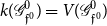 $k( \mathscr{G}_{ \mathfrak{f}^0} ^0)= V( \mathscr{G}_{ \mathfrak{f}^0} ^0)$
,
 $k( \mathscr{G}_{ \mathfrak{f}^0} ^0)-D=C_{\partial}( \mathscr{G}_{ \mathfrak{f}^0} ^0)\geq 0$
, we can check the consistency of (52) as the following makes still sense:
 \begin{equation}\mathfrak{T}_{ \mathscr{G}_{ \mathfrak{f}^0} ^0}(x,y,z,s,w,q,t)=z^{2[k( \mathscr{G}_{ \mathfrak{f}^0} ^0)-D+B_{{\textrm{ext}}}( \mathscr{G}_{ \mathfrak{f}^0} ^0)]}s^{k( \mathscr{G}_{ \mathfrak{f}^0} ^0) - D} w^{F_\partial( \mathscr{G}_{ \mathfrak{f}^0} ^0)} q^{E_\partial( \mathscr{G}_{ \mathfrak{f}^0} ^0)}\,t^{\,f( \mathscr{G}_{ \mathfrak{f}^0} ^0)}.\end{equation}
It may exist several possible reductions of the above polynomial. We will focus on the following:
 \begin{align}
&\mathfrak{T}_{ \mathscr{G}_{ \mathfrak{f}^0} } (x,y,z,z^{-2},w,q,t) = \mathfrak{T}^{\prime}_{ \mathscr{G}_{ \mathfrak{f}^0} } (x,y,z,w,q,t) \,,\nonumber\\[5pt]
& \mathfrak{T}_{ \mathscr{G}_{ \mathfrak{f}^0} } (x,y,z,z^{-2}s^{2},s^{-1},s,s^{-1}) = \mathfrak{T}^{\prime\prime}_{ \mathscr{G}_{ \mathfrak{f}^0} } (x,y,z,s)\,, \nonumber \\[5pt]
&\mathfrak{T}_{ \mathscr{G}_{ \mathfrak{f}^0} } (x,y,z,z^{2}z^{-2},z^{-1},z,z^{-1}) = \mathfrak{T}^{\prime\prime\prime}_{ \mathscr{G}_{ \mathfrak{f}^0} } (x,y,z) \,.\end{align}
Proposition 4.29 ensures that
 $\mathfrak{T}^{\prime}_{ \mathscr{G}_{ \mathfrak{f}^0} }$
is a polynomial. Meanwhile,
 $\mathfrak{T}^{\prime\prime}_{ \mathscr{G}_{ \mathfrak{f}^0} }$
is also a polynomial with exponent of s the Euler characteristics of the boundary
 $ {\partial \mathscr{G}_{ \mathfrak{f}^0 } } $
.
 $\mathfrak{T}^{\prime\prime\prime}_{ \mathscr{G}_{ \mathfrak{f}^0} } (x,y,z) $
combines both invariants in a single exponent. These polynomials will be relevant in the next analysis. Note that we could have introduced another polynomial expressed as
 $\mathfrak{T}_{ \mathscr{G}_{ \mathfrak{f}^0} } (x,y,z,s^{2},s^{-1},s,s^{-1}) = \mathfrak{T}^0_{ \mathscr{G}_{ \mathfrak{f}^0} } (x,y,z,s)$
. But this reduction turns out to satisfy the same properties as
 $\mathfrak{T}$
and thus does not provide anything new.
We are now in position to prove our main theorem.
Theorem 4.32 (Contraction/cut rule for w-coloured graphs) Let
 $ \mathscr{G}_{ \mathfrak{f}^0} $
be a rank 3 w-coloured graph. Then, for an ordinary edge e of
 $ \mathscr{G}_{ \mathfrak{f}^0} $
, we have
 \begin{equation}\mathfrak{T}_{ \mathscr{G}_{ \mathfrak{f}^0} }=\mathfrak{T}_{ \mathscr{G}_{ \mathfrak{f}^0} \vee e} +\mathfrak{T}_{ \mathscr{G}_{ \mathfrak{f}^0} /e}\,,\end{equation}
for a bridge e, we have
 $\mathfrak{T}_{ \mathscr{G}_{ \mathfrak{f}^0} \vee e}= z^8s(wq)^3t^2 \mathfrak{T}_{ \mathscr{G}_{ \mathfrak{f}^0} /e}$
and
 \begin{equation}\mathfrak{T}_{ \mathscr{G}_{ \mathfrak{f}^0} } =[(x-1)z^8s(wq)^3t^2+1] \mathfrak{T}_{ \mathscr{G}_{ \mathfrak{f}^0} /e}\,;\end{equation}
for a trivial p–inner loop e,
 $p=0,1,2$
, we have
 \begin{equation}\mathfrak{T}_{ \mathscr{G}_{ \mathfrak{f}^0} }=\mathfrak{T}_{ \mathscr{G}_{ \mathfrak{f}^0} \vee e} + (y-1)z^{4p-7}\,\mathfrak{T}_{ \mathscr{G}_{ \mathfrak{f}^0} /e}\,.\end{equation}
Proof. Let
 $ \mathscr{G}_{ \mathfrak{f}^0} $
be a rank 3 w-coloured graph. The same preliminary remarks of the proof of Theorem 3.11 hold also here for
 $ \mathscr{G}_{ \mathfrak{f}^0} $
, with adapted consideration, e.g. sHEs replace HRs. Our main concern is the change in the number of closed and open bubbles.
We concentrate first on (68). Consider an ordinary edge e of
 $ \mathscr{G}_{ \mathfrak{f}^0} $
of colour a, the set of spanning c-subgraphs which do not contain e being the same as the set of spanning c-subgraphs of
 $ \mathscr{G}_{ \mathfrak{f}^0} \vee e$
, the number of open and closed bubbles on each subgraph is the same, it is direct to get
 \begin{eqnarray}&& \sum_{A \Subset \mathscr{G}_{ \mathfrak{f}^0} ; e\notin A} (x-1)^{r( \mathscr{G}_{ \mathfrak{f}^0} )-r(A)}(y-1)^{n(A)}z^{5k(A)-[3(V- E(A))+2(F_{{\textrm{int}}}(A)-B_{{\textrm{int}}}(A)-B_{{\textrm{ext}}}(A))]} \\ && \qquad \qquad \times s^{C_\partial(A)} \, w^{F_{\partial}(A)} q^{E_{\partial}(A)} t^{\,f(A)}=\mathfrak{T}_{ \mathscr{G}_{ \mathfrak{f}^0} \vee e} .\end{eqnarray}
Let us focus on the second term of (68). Consider e, its end vertices
 $v_1$
and
 $v_2$
and its 3 strands with colour pairs
 $(aa_1)$
,
 $(aa_2)$
and
 $(aa_3)$
and consider the set of bubbles in
 $ \mathscr{G}_{ \mathfrak{f}^0} $
. Some bubbles do not use any strand of e and three bubbles can be formed using these strands (these bubbles are of colours
 $(aa_ia_j)$
,
 $i<j$
). Contracting e, the vertex obtained is connected by Lemma 4.22. The cycles and paths made of strands of e are clearly preserved after the contraction. The bubbles which use no strands of e are not affected at all by the procedure. The three bubbles using 2 strands of e are also preserved since the contraction does not delete faces. The faces passing through e getting only shortened, the result from the point of view of the bubbles passing through e is simply an ordinary ribbon edge contraction in the sense of HERGs. Using this, we write
 \begin{eqnarray}&&\sum_{A \Subset \mathscr{G}_{ \mathfrak{f}^0} ; e\in A}(x-1)^{r( \mathscr{G}_{ \mathfrak{f}^0} )-r(A)}(y-1)^{n(A)}z^{5k(A)-[3(V- E(A))+2(F_{{\textrm{int}}}(A)-B_{{\textrm{int}}}(A)-B_{{\textrm{ext}}}(A))]} \\ && \qquad \qquad \times s^{C_\partial(A)} \, w^{F_{\partial}(A)} q^{E_{\partial}(A)} t^{\,f(A)}=\mathfrak{T}_{ \mathscr{G}_{ \mathfrak{f}^0} /e} .\end{eqnarray}
Let us focus now on the bridge case and (69). Cutting a bridge yields, as in the ordinary case, from the sum
 $\sum_{A \Subset \mathscr{G}_{ \mathfrak{f}^0} ; e\notin A}$
the product
 $(x-1)\mathfrak{T}_{ \mathscr{G}_{ \mathfrak{f}^0} \vee e}$
. The second sum remains as it is using the mapping between
 $\{A \Subset \mathscr{G}_{ \mathfrak{f}^0} ;e\in A\}$
and
 $\{A\Subset \mathscr{G}_{ \mathfrak{f}^0} /e\}$
and provided the fact that the resulting vertex is still connected. That is, once again, ensured by Lemma 4.22. The last stage relates
 $\mathfrak{T}_{ \mathscr{G}_{ \mathfrak{f}^0} \vee e}$
and
 $\mathfrak{T}_{ \mathscr{G}_{ \mathfrak{f}^0} /e}$
. This can be achieved by using the bijection between
 $A\Subset \mathscr{G}_{ \mathfrak{f}^0} \vee e$
and
 $A' \Subset \mathscr{G}_{ \mathfrak{f}^0} /e$
where each A and A
′ are both uniquely related to some
 $A_0\Subset \mathscr{G}_{ \mathfrak{f}^0} $
as
 $A = A_0\vee e$
and
 $A'=A_0/e$
. Using Lemma 4.26, the relation (69) follows.
Next, we discuss the trivial p–inner loop case and prove (70). The property (71) should be direct. The second term in (70) is now studied.
The question is whether or not e being a trivial p–inner loop in
 $ \mathscr{G}_{ \mathfrak{f}^0} $
remains as such in A. The answer for that question is yes because A contains the end vertex of e. We may cut some edges in each sectors
 $v_i$
(see Figure 29) for defining A but the resulting sectors are distinct in A.
Contracting a trivial p–inner loop generates p circles and
 $3-p$
non-trivial vertices. Now, from Lemma 4.24, we know how all numbers of components in the graph evolve: the nullity is again
 $n(A) = n\big(A'\big) + 1$
, and the exponent of z becomes
 \begin{align}
&5k(A) - (3(V( \mathscr{G}_{ \mathfrak{f}^0} ) - E(A)) + 2(F_{\textrm{int}}(A) - B_{\textrm{int}}(A)-B_{{\textrm{ext}}}(A)) = \nonumber\\[5pt]
&5(k\big(A'\big)-2) - \Big[3[V( \mathscr{G}_{ \mathfrak{f}^0} /e)-2) - (E\big(A'\big)+1)] + 2(F_{\textrm{int}}\big(A'\big) - B_{\textrm{int}}\big(A'\big)-B_{{\textrm{ext}}}\big(A'\big)+\alpha_p)\Big]\nonumber\\[5pt]
& = 5k\big(A'\big) - (3(V( \mathscr{G}_{ \mathfrak{f}^0} /e) - E\big(A'\big)) + 2(F_{\textrm{int}}\big(A'\big) - B_{\textrm{int}}\big(A'\big)-B_{{\textrm{ext}}}\big(A'\big)) -7 +4p \,,\end{align}
where
 $\alpha_p=3-2p$
, A and A
′ refer to the subgraphs related by bijection the usual between spanning c-subgraphs of
 $\{A \Subset \mathscr{G}_{ \mathfrak{f}^0} ;e\in A\}$
and
 $\{A'\Subset \mathscr{G}_{ \mathfrak{f}^0} /e\}$
. At the end, one gets
 $(y-1)z^{4p-7}\mathfrak{T}_{ \mathscr{G}_{ \mathfrak{f}^0} /e}$
.
We realize again that the relations of Theorem 4.32 are not complete reduction rules. General boundary conditions as generalized bouquets must be explicitly computed using Definition 4.27.
Corollary 4.33 (Cut/contraction relations for
 $\mathfrak{T}'$
) Let
 $ \mathscr{G}_{ \mathfrak{f}^0} $
be a rank 3 w-coloured graph. Then, for a bridge e, we have
 $\mathfrak{T}^{\prime}_{ \mathscr{G}_{ \mathfrak{f}^0} \vee e}= z^{6}(wq)^3t^2 \mathfrak{T}^{\prime}_{ \mathscr{G}_{ \mathfrak{f}^0} /e}$
and
 \begin{equation}\mathfrak{T}^{\prime}_{ \mathscr{G}_{ \mathfrak{f}^0} }(x,y,z,w,q,t) =[(x-1)z^6(qw)^3t^2+1] \mathfrak{T}^{\prime}_{ \mathscr{G}_{ \mathfrak{f}^0} /e}(x,y,z,w,q,t)\,;\end{equation}
for a trivial p–inner loop e in
 $ \mathscr{G}_{ \mathfrak{f}^0} $
,
 $0\leq p \leq 2$
, we have
 \begin{equation}\mathfrak{T}^{\prime}_{ \mathscr{G}_{ \mathfrak{f}^0} }(x,y,z,1,q,t)=z^{4p-6} [q^3t^2+ (y-1)z^{-1}]\,\mathfrak{T}^{\prime}_{ \mathscr{G}_{ \mathfrak{f}^0} /e}(x,y,z,1,q,t)\,;\end{equation}
Proof. Theorem 4.32 implies naturally (74) after the setting
 $s=z^{-2}$
in
 $\mathfrak{T}_{ \mathscr{G}_{ \mathfrak{f}^0} }$
. We now work out the contraction/cut of the trivial loops.
Same arguments as in the proof of Theorem 4.32 should be invoked here. The difference now is that, by changing
 $s\to z^{-2}$
, using
-
1. the one-to-one mapping between
$\{A \Subset \mathscr{G}_{ \mathfrak{f}^0} \vee e\}$
and
$\{A' \Subset \mathscr{G}_{ \mathfrak{f}^0} /e \}$
such that with each
$A \Subset \mathscr{G}_{ \mathfrak{f}^0} \vee e$
one associates
$A' \Subset \mathscr{G}_{ \mathfrak{f}^0} /e$
defined by
$A'=\tilde A/e$
,
$\tilde A\Subset \mathscr{G}_{ \mathfrak{f}^0} $
, and
$\tilde A \vee e = A$
and


we can map, for a trivial 0, 1, 2–inner loop e,
 $\mathfrak{T}_{ \mathscr{G}_{ \mathfrak{f}^0} \vee e}$
on
 $\mathfrak{T}_{ \mathscr{G}_{ \mathfrak{f}^0} /e}$
. We compute the variation of the exponent of z between A and A
′ as
 \begin{align}
&5k(A) - (3(V( \mathscr{G}_{ \mathfrak{f}^0} ) - E(A)) + 2[F_{\textrm{int}}(A) +C_\partial(A)- B_{\textrm{int}}(A)- B_{{\textrm{ext}}}(A)]) =\nonumber\\[5pt]
&5(k\big(A'\big)- 2 )- (3(V( \mathscr{G}^{\,\prime}_{ \mathfrak{f}^0})-2-E\big(A'\big)) + 2[F_{\textrm{int}}\big(A'\big) +C_\partial\big(A'\big)-2-B_{\textrm{int}}\big(A'\big) - B_{\textrm{ext}}\big(A'\big) + \alpha_p ])\nonumber\\[5pt]
& = 5k\big(A'\big) - (3(V( \mathscr{G}_{ \mathfrak{f}^0} /e) - E\big(A'\big)) + 2[F_{\textrm{int}}\big(A'\big) - B_{\textrm{int}}\big(A'\big) - B_{\textrm{ext}}\big(A'\big)]) -2\alpha_p \,.\end{align}
The rest of the variations can be easily identified using the same lemma.
Corollary 4.34 (Cut/contraction rules for
 $\mathfrak{T}''$
(and
 $\mathfrak{T}'''$
)) Let
 $ \mathscr{G}_{ \mathfrak{f}^0} $
be a rank 3 w-coloured graph.
Then, for a bridge e, we have
 $\mathfrak{T}^{\prime\prime}_{ \mathscr{G}_{ \mathfrak{f}^0} \vee e} = z^{6}\mathfrak{T}^{\prime\prime}_{ \mathscr{G}_{ \mathfrak{f}^0} /e}$
and
 \begin{equation}\mathfrak{T}^{\prime\prime}_{ \mathscr{G}_{ \mathfrak{f}^0} } =[ (x-1)z^6 + 1]\,\mathfrak{T}^{\prime\prime}_{ \mathscr{G}_{ \mathfrak{f}^0} /e}\,;\end{equation}
for a trivial p–inner loop e in
 $ \mathscr{G}_{ \mathfrak{f}^0} $
,
 $0\leq p \leq 2$
, we have
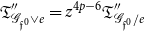 $\mathfrak{T}^{\prime\prime}_{ \mathscr{G}_{ \mathfrak{f}^0} \vee e} =z^{4p-6} \mathfrak{T}^{\prime\prime}_{ \mathscr{G}_{ \mathfrak{f}^0} /e}$
and
 \begin{equation}\mathfrak{T}^{\prime\prime}_{ \mathscr{G}_{ \mathfrak{f}^0} }= z^{4p-6}[1+ (y-1)z^{-1}]\,\mathfrak{T}^{\prime\prime}_{ \mathscr{G}_{ \mathfrak{f}^0} /e}\,.\end{equation}
The same contraction and cut rules applies for
 $\mathfrak{T}^{\prime\prime\prime}_{ \mathscr{G}_{ \mathfrak{f}^0} }$
.
Proof. The new ingredient to achieve the proof of this statement is (41) of Lemma 4.26.
The exponents of
 $z^{4p-7}$
or of
 $z^{4p-6}$
can be negative in some cases. This simply implies that, in the polynomial
 $\mathfrak{T}^{\prime}_{ \mathscr{G}_{ \mathfrak{f}^0} /e}$
or
 $\mathfrak{T}^{\prime\prime}_{ \mathscr{G}_{ \mathfrak{f}^0} /e}$
, all monomials should contain an enough large power of z to make the overall exponent of z positive.
The disjoint union operation on graph extends naturally in the present formulation.
Lemma 4.35 (Disjoint union). Let
 $ \mathscr{G}_{ \mathfrak{f}^0} $
and
 $ \mathscr{G}^{\,\prime}_{ \mathfrak{f}^0} $
two disjoint rank 3 w-coloured graphs, then
 \begin{equation}\mathfrak{T}_{ \mathscr{G}_{ \mathfrak{f}^0} \sqcup \mathscr{G}^{\,\prime}_{ \mathfrak{f}^0}} =\mathfrak{T}_{ \mathscr{G}_{ \mathfrak{f}^0} } \, \mathfrak{T}_{ \mathscr{G}^{\,\prime}_{ \mathfrak{f}^0}} \,.\end{equation}
Proof. This is totally standard as in the ordinary procedure using additive properties of exponents in
 $\mathfrak{T}_{ \mathscr{G}_{ \mathfrak{f}^0} }$
.
Corollary 4.36 (3–inner loop contraction) Given a rank 3 w-coloured graph
 $ \mathscr{G}_{ \mathfrak{f}^0} $
containing a 3–inner loop e then
 \begin{equation}\mathfrak{T}_{ \mathscr{G}_{ \mathfrak{f}^0} } = z^5\left(z^3s(wq)^3t^2 + y-1\right) \mathfrak{T}_{ \mathscr{G}_{ \mathfrak{f}^0} /e}\,.\end{equation}
Proof. We use the fact that e is a 3–inner and so it forms a separate subgraph g. In order to compute the polynomial of
 $ \mathscr{G}_{ \mathfrak{f}^0} $
, Lemma 4.35 can be applied and a direct evaluation of g yields the desired factor.
Definition 4.37 (Multivariate form). The multivariate form associated with (52) is defined by:
 \begin{align}
&\widetilde{\mathfrak{T}}_{ \mathscr{G}_{ \mathfrak{f}^0} }(x,\{\beta_e\},\{z_i\}_{i=1,2,3},s,w,q,t) =\nonumber\\[6pt]
& \sum_{A \Subset \mathscr{G}_{ \mathfrak{f}^0} } x^{r(A)}\left(\prod_{e\in A}\beta_e\right)z_1^{F_{{\textrm{int}}}(A)}z_2^{B_{{\textrm{int}}}(A)} z_3^{B_{{\textrm{ext}}}(A)}\,s^{C_\partial(A)} \, w^{F_{\partial}(A)} q^{E_{\partial}(A)} t^{\,f(A)}\,,\end{align}
for
 $\{\beta_e\}_{e\in \mathcal{E}}$
labelling the edges of the graph
 $ \mathscr{G}_{ \mathfrak{f}^0} $
.
It is direct to prove the following statement by ordinary techniques.
Proposition 4.38. For any ordinary edge e,
 \begin{eqnarray} \widetilde{\mathfrak{T}}_{ \mathscr{G}_{ \mathfrak{f}^0} }=\widetilde{\mathfrak{T}}_{ \mathscr{G}_{ \mathfrak{f}^0} \vee e} +x\beta_e\,\widetilde{\mathfrak{T}}_{ \mathscr{G}_{ \mathfrak{f}^0} /e}\,.\end{eqnarray}
Remark 4.39 We can compare
 $\widetilde{\mathfrak{T}}$
with the Gurau polynomial denoted in the following by G [Reference Gurau20]. Note that we will not use the full form of
 $G_{ \mathscr{G}_{ \mathfrak{f}^0} }$
, denoted
 $P_{ \mathscr{G}_{ \mathfrak{f}^0} }$
in [Reference Gurau20], but will instead introduce two improvements: (1) a normalization form
 $P_{ \mathscr{G}_{ \mathfrak{f}^0} }(\{\beta_e x_1\},\dots)$
of
 $P_{ \mathscr{G}_{ \mathfrak{f}^0} }$
, where
 $x_1$
is the variable associated with the number of edges which brings an inessential overall factor of
 $x_1^{E(A)}$
consistently absorbed by the
 $\beta_e$
, and (2) a rank formulation of
 $G_{ \mathscr{G}_{ \mathfrak{f}^0} }(\{\beta_e\},\dots) =P_{ \mathscr{G}_{ \mathfrak{f}^0} }(\{\beta_e x_1\},\dots)$
, i.e. rather then using two variables
 $x_0$
for the vertices and
 $x_4$
for the number of connected components of the rank 3 coloured tensor graph, we simply use
 $x^{r(A)}$
,
 $A \Subset \mathscr{G}_{ \mathfrak{f}^0} $
.
For a rank 3 coloured tensor graph
 $ \mathscr{G}_{ \mathfrak{f}^0} $
, the polynomials
 $\widetilde{\mathfrak{T}}$
and G are related by
 \begin{equation}\widetilde{\mathfrak{T}}_{ \mathscr{G}_{ \mathfrak{f}^0} }(x,\{\beta_e\}, z_1,z_2,z_3=1,s,w,q,t) = G_{ \mathscr{G}_{ \mathfrak{f}^0} }(x,\{\beta_e\},z_1,z_2,s,q,w,t)\,,\end{equation}
with, according to the convention in [Reference Gurau20], we have
 \begin{eqnarray}C_\partial = |\mathfrak{B}_{\partial}^3|, \quad F_\partial = |\mathfrak{B}_{\partial}^2|, \quad E_\partial = |\mathfrak{B}_{\partial}^1|, \quad f = |\mathfrak{B}_{\partial}^0|, \quad B_{{\textrm{int}}}= |\mathfrak{B}^3|, \quad F_{{\textrm{int}}} = |\mathfrak{B}^2|.\end{eqnarray}
As expected, for this set of graphs the polynomial
 $\widetilde{\mathfrak{T}}$
is more general because it contains one additional variable (
 $z_3$
fixed to 1) associated with the number of open bubbles. This variable can be introduced by hand in G making it a bit more general. This additional variable does not lead to any new features for the multivariate form however, as seen in our developments, it plays an important role in the non-multivariate form
 $\mathfrak{T}$
.
5. Conclusion
We have generalized the Tutte and BR polynomials to rank 3 w-coloured graphs. The rank D w-coloured graphs are new combinatorial objects obtained from the (stranded) edge contraction of rank D half-edged, coloured and stranded graphs. Coloured stranded and tensor graphs have appeared in several contexts in physics, in particular, as Feynman graphs of field theories describing quantum geometry and gravity. The new polynomial invariant
 $\mathfrak{T}$
presented in this work satisfies a contraction/cut recursion relation on rank 3 w-coloured graphs, with the cut operation which seems natural in this context. We have evaluated some boundary cases or terminal forms of the contraction/cut recursion relation for these graphs. The multivariate form of the invariant has been given, and its relation with the Gurau polynomial, see [Reference Gurau20], has been established.
Studying the limit cases, the invariant
 $\mathfrak{T}$
reduces to the Tutte polynomial on its underlying graph. The connection with the BR polynomial on half-edged ribbon graphs might be also achieved after reduction of the present analysis to rank 2.
The perspectives of this work are numerous. First, we must mention that it is not excluded that rank D w-coloured graphs and all other graph species studied in this work find other definitions. For instance, there is another interesting underlying graph of an HESG
 $ \mathscr{G} _{\mathfrak{f}^0}$
. The string graph
 $S( \mathscr{G} _{\mathfrak{f}^0})$
of
 $ \mathscr{G} _{\mathfrak{f}^0}$
is the graph whose vertex set is the set of vertex points and SHe external points of
 $ \mathscr{G} _{\mathfrak{f}^0}$
, and whose edge set is the set of strands and chords in
 $ \mathscr{G} _{\mathfrak{f}^0}$
, the incidence relation between the vertices and edges of
 $S( \mathscr{G} _{\mathfrak{f}^0})$
being obvious. Appearing as a watermark in Definition 4.6, such a graph that might reveal a new point of view and perhaps brings simplification of the present results. This is certainly worth investigating.
For instance, the universality property of
 $\mathfrak{T}$
must be addressed, once the notion of the one-vertex w-coloured graphs is well mastered. The introduction of colours might help in classifying the bouquets of w-coloured graphs needed in this proof. In fact, before addressing the universality issue on stranded structures, one first needs to understand to how the universality property can be extended for the extension of the BR polynomial to HERGs. This will amount to generalizing the notion of chord diagrams
 $\mathcal{D}$
, their equivalence relation under rotations about chords, and finally their associated basic canonical diagrams
 $\mathcal {D}_{ijk}$
(counting the nullity i, genus j of the diagram, k is associated with the orientation of the surface associated with diagram) [Reference Bollobás8, Reference Bollobás and Riordan10] to chord diagrams with half-edges. Such a preliminary task will certainly imply the existence of a new canonical diagram
 $\mathcal {D}_{ijkl}$
, where i, j, k keep their meaning, and l defines the number of connected components associated with the boundary of the HERG. It is also known that the Tutte and BR polynomials can be expressed in terms of spanning tree expansions and enumerate specific trees. We may ask: what type of tree expansion does
 $\mathfrak{T}$
satisfy, and which objects does it enumerate? These new lines of investigation will certain yield interesting results relating combinatorics and topology in higher dimension [Reference Avohou, Ben Geloun and Nuwagira4].
Finally, the study of tensor graphs have been motivated by their importance in quantum gravity. A natural follow up question might be what are the new information brought by the new class of w-coloured graphs or the new polynomial invariant
 $\mathfrak{T}$
in that context? An answer of this question is not obvious. However, in the search of new tools for classifying the Feynman graphs which are viewed as random manifolds, the following investigation tracks might be relevant to address. First, each colour in the field theoretic setting represents a different field, and the path integral in a field theory integrates over field configurations. Integrating over a colour makes the resulting Feynman graph independent of it. Practically, we use an edge contraction to represent the new Feynman graph. This procedure has been used by Bonzom et al. [Reference Bonzom, Gurau and Rivasseau12] to reveal a new class of objects called uncoloured graphs. Uncoloured Feynman graphs are coloured tensor graphs on which we perform edge contractions, for all edge colours except for one. It could be therefore timely to investigate in which sense w-coloured graphs are interpolating configurations between a fully coloured tensor theory by Gurau and an uncoloured one in the sense of Bonzom et al., and making perhaps the formalism developed therein a bit more general. Furthermore, to find a practical use of the new invariant
 $\zeta( \mathscr{G}_{ \mathfrak{f}^0} )$
found in the present work, one must first interpret, at the level of the dual simplicial complex, the meaning of the contraction, and the cut procedure performed at the level of the w-coloured graph. Thus, another possible investigation is to understand dualities at the level of graphs and simplicial complexes (with boundaries), and consequently dualities satisfied by the polynomial
 $\mathfrak{T}$
itself. This hopefully could lead to a better understanding of simplicial complexes generated by path integrals.
Acknowledgements
Discussions with Vincent Rivasseau at early stage of this work are gratefully acknowledged. RCA thanks the Perimeter Institute for its hospitality and support in the time that this work had been initiated. This work is supported by TWAS Research Grant RGA No. 17-542 RG/MATHS/AF/AC_G -FR3240300147.The ICMPA-UNESCO Chair is in partnership with Daniel Iagolnitzer Foundation (DIF), France, and the Association pour la Promotion Scientifique de l’Afrique (APSA), supporting the development of mathematical physics in Africa.
Appendix: Examples
We carry out explicitly two examples in order to illustrate our results in the present appendix.
Example 1:
A coloured graph. Consider the graph
 $ \mathscr{G} $
given by Figure A.1. Computing the multivariate form of the polynomial by the spanning c-subgraph summation in (81) with
 $\beta_i$
is associated with the edge of colour i, we obtain A.
 \begin{align}\mathfrak{T}_{ \mathscr{G} }(x,\{\beta_e\},z,s,q,t) =\, & \beta_0\beta_1\beta_2\beta_3\, xz_1^6z_2^4\nonumber \\[5pt]
&+( \beta_0\beta_1\beta_2 + \beta_0\beta_2\beta_3 + \beta_1\beta_2\beta_3 + \beta_0\beta_1\beta_3)\, x z_1^3 z_2z_3^3sw^{3}q^3t^2\nonumber \\[5pt]
&+ ( \beta_0\beta_1 + \beta_0\beta_2 + \beta_0\beta_3 + \beta_1\beta_2 + \beta_1\beta_3 + \beta_2\beta_3)\, xz_1z_3^{4} sw^{4}q^6t^4\nonumber \\[5pt]
&+ ( \beta_0 + \beta_1 + \beta_2 + \beta_3)\,xz_3^{5}s w^{5} q^9t^6 + z_3^{8}s^2w^8q^{12}t^8\,.\end{align}
Then this polynomial coincides exactly with the normalized Gurau polynomial
 $G_{ \mathscr{G} }$
after setting to 1 the variable
 $z_3$
associated with open bubbles. Note that reversely, introducing a new variable associated with the same component in
 $G_{ \mathscr{G} }$
, we infer that both polynomials match for the present example. Note also that the exponents of
 $z_3$
and w always coincide. It is, however, not always true that each open bubble would have a unique boundary component.
A rank 3 coloured tensor graph
 $ \mathscr{G} $
and its cut
 $ \mathscr{G} \vee e$
and contraction
 $ \mathscr{G} /e$
for an ordinary edge e of colour 2.

Cutting one edge, say the one of colour 0, yields
 $ \mathscr{G} \vee e$
, so that we evaluate
 \begin{align}
\mathfrak{T}_{ \mathscr{G} \vee e}(x,\{\beta_e\},z,s,q,t)=\, & \beta_1\beta_2\beta_3\, xz_1^3 z_2 z_3^{3} sw^3q^{3} t^2 \nonumber\\[5pt]
&+( \beta_1\beta_2 + \beta_1\beta_3 + \beta_2\beta_3)xz_1z_3^{4} sw^4q^{6}t^4 \nonumber\\[5pt]
&+ ( \beta_1 + \beta_2 + \beta_3)xz_3^{5}sw^5q^{9}t^6 + z_3^{8}s^2w^{8} q^{12}t^8\end{align}
and contracting the same edge gives
 \begin{align}
\mathfrak{T}_{ \mathscr{G} /e}(x,\{\beta_e\},z,s,q,t)=\, &\beta_1\beta_2\beta_3\, z_1^6 z_2^4 \nonumber\\[5pt]
&+ ( \beta_1\beta_2 + \beta_2\beta_3 + \beta_1\beta_3)z_1^3 z_2z_3^{3} sw^{3} q^3t^2 \nonumber\\[5pt]
&+ (\beta_1 + \beta_2 + \beta_3)z_1z_3^{4}sw^4q^{6}t^4 + z_3^{5}sw^5q^{9}t^6\,.\end{align}
Thus, we get
 \begin{eqnarray} \mathfrak{T}_{ \mathscr{G} }=\mathfrak{T}_{ \mathscr{G} \vee e} +x\beta_0\mathfrak{T}_{ \mathscr{G} /e}\,.\end{eqnarray}
It should be also emphasized that the contraction of an edge is performed in the sense of Definition 4.7. This definition allows us to improve the active/passive contraction scheme as used in [Reference Gurau20].
Example 2:
A “planar” w-coloured graph. We can compute
 $\mathfrak{T}$
for other types of graphs which are not coloured tensor graphs. In a specific instance, consider the graph
 $ \mathscr{G}_{ \mathfrak{f}^0} $
of Figure 32. It combines both one coloured vertex and another type vertex. For simplicity, we change the variables
 $(x-1) \to x$
and
 $(y-1) \to y$
.
By the spanning c-subgraph summation, we get
 \begin{eqnarray}\mathfrak{T}_{ \mathscr{G}_{ \mathfrak{f}^0} }(x,y,z,s,q,t) = [ x z^{10} s w^5q^{9} t^{6}+ xyz^{9} s w^{4}q^{6} t^{4} + 2z^2w^2q^{6} t^{4}+ 3yzw q^{3} t^{2} + y^2 ] z^{14}sw^5q^9t^{6} \,.\nonumber\\
\end{eqnarray}
We want to compare (A.5) with the result obtained by contraction and cut procedure using a much as possible results on terminal forms. Using the notation of Figure A.2, we must check that
 \begin{equation}\mathfrak{T}_{ \mathscr{G}_{ \mathfrak{f}^0} } = \mathfrak{T}_{ \mathscr{G}_{ \mathfrak{f}^0} \vee e_2} +\mathfrak{T}_{ \mathscr{G}_{ \mathfrak{f}^0} /e_2} \,.\end{equation}
Evaluating
 $ \mathfrak{T}_{ \mathscr{G}_{ \mathfrak{f}^0} \vee e_2}$
and
 $\mathfrak{T}_{ \mathscr{G}_{ \mathfrak{f}^0} /e_2}$
, one finds
 \begin{eqnarray}&&\mathfrak{T}_{ \mathscr{G}_{ \mathfrak{f}^0} \vee e_2}= [x z^8s(wq)^3t^2 + 1 ]\mathfrak{T}_{( \mathscr{G}_{ \mathfrak{f}^0} \vee e_2)/e_0}\,,\quad \mathfrak{T}_{( \mathscr{G}_{ \mathfrak{f}^0} \vee e_2)/e_0} = \mathfrak{T}_{(( \mathscr{G}_{ \mathfrak{f}^0} \vee e_2)/e_0)\vee e_1}+ y z \, \mathfrak{T}_{(( \mathscr{G}_{ \mathfrak{f}^0} \vee e_2)/e_0)/e_1}\,, \end{eqnarray}
 \begin{eqnarray}&&\mathfrak{T}_{ \mathscr{G}_{ \mathfrak{f}^0} /e_2} = \mathfrak{T}_{( \mathscr{G}_{ \mathfrak{f}^0} /e_2) \vee e_1} + yz\,\mathfrak{T}_{( \mathscr{G}_{ \mathfrak{f}^0} /e_2)/e_1}\,.\end{eqnarray}
We used in (A.7) the fact that
 $e_0$
is a bridge in
 $ \mathscr{G}_{ \mathfrak{f}^0} \vee e_2$
and that
 $e_1$
is a 2–inner loop in
 $( \mathscr{G}_{ \mathfrak{f}^0} \vee e_2)/e_0$
. Meanwhile, in (A.8), we used the fact that
 $e_1$
is a 2–inner loop in
 $ \mathscr{G}_{ \mathfrak{f}^0} /e_2$
.
A straightforward calculation yields
 \begin{eqnarray}&& \mathfrak{T}_{(( \mathscr{G}_{ \mathfrak{f}^0} \vee e_2)/e_0)\vee e_1}= z^{16}sw^7q^{15} t^{10}\,,\qquad \mathfrak{T}_{(( \mathscr{G}_{ \mathfrak{f}^0} \vee e_2)/e_0)/e_1}= z^{14}sw^{6}q^{12} t^{8}\,, \\
&& \mathfrak{T}_{( \mathscr{G}_{ \mathfrak{f}^0} /e_2) \vee e_1} = z^{16}sw^{7}q^{15} t^{10} + yz^{15}sw^6q^{12} t^{8}\,,\qquad \mathfrak{T}_{( \mathscr{G}_{ \mathfrak{f}^0} /e_2)/e_1} = z^{14}sw^{6}q^{12} t^{8} + yz^{13}sw^{5}q^{9} t^{6}\,.\end{eqnarray}
Plugging these results on (A.7) and (A.8), and summing their contributions in (A.6), allow us to recover (A.5).
A w-coloured graph
 $ \mathscr{G}_{ \mathfrak{f}^0} $
, the cut graph
 $ \mathscr{G}_{ \mathfrak{f}^0} \vee e_2$
and the contracted graph
 $ \mathscr{G}_{ \mathfrak{f}^0} /e_2$
with respect to
 $e_2$
.