II. CNT-DIPOLES

CNT grown by means of common technology are located normally to the substrate. We are analyzing the method of computing diffraction characteristics of N CNT-dipoles located normally at the substrate in random order. In this work, we are analyzing CNTs arranged in dielectric with dielectric permeability $\varepsilon _1 $ normal to a dielectric substrate $\varepsilon _2 $, $\mu _1=\mu _2=1$. We introduce a rectangular coordinate system with X, Y axes parallel to the substrate and normal to CNT and Z-axis directed along the dipole and normal to the substrate. The origin of coordinates is lying on the substrate. The length of the CNT is L and radius is a.

We consider that the following boundary condition is correct on the surface of the dipole:

(1)$$E_z=\rho _S \;j\comma \; $$

where E _z, j are the longitudinal components of electric field intensity and surface current density, ρ _S is the surface resistance of CNT [Reference Hanson3, Reference Slepyan, Shuba, Maksimenko and Lakhtakia4],$\, \rho _s=i\lpar \pi ^2 a\hbar \lpar \omega - i\nu \rpar /2e^2 \upsilon _{\rm F} \rpar $, $\upsilon _{\rm F} $ is the Fermi velocity (for CNT $\upsilon _F=9.71 \times 10^5 \; {\rm m}/{\rm s}$), $\omega $ is the cyclic frequency, $\nu $ is the relaxation frequency (for CNT $\nu=3.33 \times 10^{11} $Hz), e is the electron charge, c is the velocity of light in free space, and $\hbar $ is the Planck constant.

At first, we analyze a single CNT-dipole. We consider that only a longitudinal component of the current exists on the dipole and depends only on z. We use boundary condition (1). As a result, we derive the following expression:

(2)$$\eqalign{& \displaystyle{1 \over {i\omega \varepsilon _1 \varepsilon _0 }}\left({\displaystyle{{d^2 } \over {dz^2 }}+k_1 ^2 } \right)\int_0^L {j\lpar z^{\prime}\rpar } g_e \lpar z\comma \; z^{\prime}\rpar dz^{\prime}+E_z^e \left(z \right)\comma\cr & \quad =\rho _s j\left(z \right)\comma \; \, z \in \left[{0\comma \; \, L} \right]} \; $$

where k ₁ is the wave number in upper dielectric, the core of the IDE $g_e \lpar z\comma \; z^{\prime}\rpar $ is defined below.

We consider external field $E_z^e \lpar z\rpar $ as the sum of two planе waves – incident wave and wave reflected from the substrate without dipole. The reflection coefficient is defined by the Fresnel formula. The vector of $\vec E^e \lpar z\rpar $ is in the plane of incidence.

The kernel of the IDE

(3)$$g_e \lpar z\comma \; z^{\prime}\rpar =\displaystyle{a \over {2\pi }}\int_0^{2\pi } {{\rm d}\phi \int_0^{2\pi } {g\lpar x\comma \; x^{\prime}\comma \; y\comma \; y^{\prime}\comma \; z\comma \; z^{\prime}\rpar } {\rm d}\phi ^{\prime}} .$$

In expression (3), we consider that the observation point and the source point are lying on the surface of the dipole:

(4)$$x=a\cos \phi\comma \; \, y=a\sin \phi\comma \; \, x^{\prime}=a\cos \phi ^{\prime}\comma \; \, y^{\prime}=a\sin \phi ^{\prime}.$$

In expression (3), the function$g\lpar x\comma \; x^{\prime}\comma \; y\comma \; y^{\prime}\comma \; z\comma \; z^{\prime}\rpar $ is the GF for the vector potential in case the current direction is normal to the surface:

(5)$$\eqalign{& \left({\displaystyle{{\partial ^2 } \over {\partial \, x^2 }}+\displaystyle{{\partial ^2 } \over {\partial \, y^2 }}+\displaystyle{{\partial ^2 } \over {\partial \, z^2 }}+k^2 \varepsilon } \right)g\lpar x\comma \; x^{\prime}\comma \; y\comma \; y^{\prime}\comma \; z\comma \; z^{\prime}\rpar \cr & \quad =- \delta \left({x - x^{\prime}} \right)\delta \left({y - y^{\prime}} \right)\delta \left({z - z^{\prime}} \right).}$$

Let$\, z^{\prime} \geq 0$. For $z \geq 0$ we will retrieve the solution of (5) in the following form:

(6)$$\eqalign{ g\lpar x\comma \; x^{\prime}\comma \; y\comma \; y^{\prime}\comma \; z\comma \; z^{\prime}\rpar &\!=\!\displaystyle{1 \over {8\pi ^2 }}\int_{ - \infty }^\infty \int_{ - \infty }^\infty \left[e^{ - \gamma _1 \left\vert {z - z^{\prime}} \right\vert} \right. \left.+\;Q\left(\rho \right)\, e^{ - \gamma _1 \lpar z+z^{\prime}\rpar } \right]\cr & \quad\times\displaystyle{1 \over {\gamma _1 }}e^{i\alpha \, \bar x+i\beta \, \bar y} d\alpha d\beta.} $$

Following notations are used here and further $\bar x=x - x^{\prime}\comma \; \; \bar y=y - y^{\prime}$, 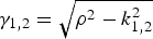$\gamma _{1\comma 2}=\sqrt {\rho ^2 - k_{1\comma 2}^2 } $, 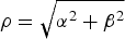$\rho=\sqrt {\alpha ^2+\beta ^2 } $, _k2 is the wave number in the substrate, $Q=\gamma _1 - \gamma _2 \, t/\gamma _1+\gamma _2 \, t$, $t=\varepsilon _1 /\varepsilon _2 .$

The first term in (6) is a partial solution of an inhomogeneous equation (5) or in other words it is free-space GF:

$$g_0 \lpar x\comma \; x^{\prime}\comma \; y\comma \; y^{\prime}\comma \; z\comma \; z^{\prime}\rpar =\displaystyle{{e^{ - ik_1 R} } \over {4\pi R}}.$$

The following integral representation is valid for it:

(7)$$\displaystyle{{e^{ - ik_1 R} } \over {4\pi R}}=\displaystyle{1 \over {4\pi ^2 }}\int_{ - \infty }^\infty {K_0 \left({R_1 \sqrt {\rho ^2 - k_1 ^2 } } \right)e^{ - i\rho \left({z - z^{\prime}} \right)} d\rho\comma \; } $$

where K ₀ is the Macdonald function.

The second term includes the substrate influence. For $\varepsilon _1=\varepsilon _2 $, $g_1=0$:

(8)$$\eqalign{& g_2 \lpar x\comma \; x^{\prime}\comma \; y\comma \; y^{\prime}\comma \; z\comma \; z^{\prime}\rpar \cr & \quad =\displaystyle{1 \over {8\pi ^2 }}\int_{ - \infty }^\infty {\int_{ - \infty }^\infty} Q\left(\rho \right)\, e^{- \gamma_1 \lpar z+z^{\prime}\rpar } \displaystyle{1 \over {\gamma _1 }}e^{i\alpha \, \bar x+i\beta \, \bar y} d\alpha d\beta} $$

We substitute expressions (7) and (8) in (3), taking into account (4) and making the change of variables $\alpha=\rho \cos \vartheta\comma \; \, \beta=\rho \sin \vartheta $. As a result we obtain the following equation:

(9)$$g_e \lpar z\comma \; z^{\prime}\rpar =g_{e\comma 1} \lpar z\comma \; z^{\prime}\rpar +g_{e\comma 2} \lpar z\comma \; z^{\prime}\rpar \comma \; $$

(10)$$g_{e\comma \, 1} \lpar z\comma \; z^{\prime}\rpar =\displaystyle{a \over {2\pi }}\int_{ - \infty }^\infty {I_0 \left({a\gamma _1 } \right)K_0 \left({a\gamma _1 } \right)e^{ - i\rho \left({z - z^{\prime}} \right)} d\rho\comma \; } $$

(11)$$g_{e\comma \, 2} \lpar z\comma \; z^{\prime}\rpar =\displaystyle{a \over {2\pi }}\int_0^\infty {\rho \, Q\left(\rho \right)\, \displaystyle{{e^{ - \gamma _1 \lpar z+z^{\prime}\rpar } } \over {\gamma _1 }}J_0^2 \left({\rho \, a} \right)} \, d\rho\comma \; $$

J ₀ is the Bessel function, I ₀ is the modified Bessel function.

We retrieve the solution of (2) using the Galerkin method

(12)$$j\left(z \right)=\sum\limits_{n=0}^\infty {X{}_n\, V_n \left(z \right)}\comma \; $$

X _n is the unknown coefficient, V _n(z) is the basis function, in whose capacity we use weighted Chebyshev polynomials of the second order:

(13)$$\eqalign{ V_n \left(z \right)&=\displaystyle{{i^n } \over {\pi \left({n+1} \right)}}\sqrt {1 - {{z^2 } / {l^2 \, }}} U_n \left({\displaystyle{z \over l}} \right)\comma \; \, \quad \cr & \quad n=0\comma \; 1\comma \; 2 \ldots.}$$

Fourier transformation of V _n(z)is expressed in terms of Bessel functions $\tilde V_n \lpar \gamma \rpar ={{J_{n+1} \lpar \gamma \, l\rpar } / \gamma }$. Substituting the current from (12) into (2) and then projecting equation (2) onto $V_{_p }^\ast \lpar z\rpar $ we obtain the system of linear algebraic equations (SLAE):

$$\sum\limits_{n=0}^\infty {X{}_n\, A_{pn}=}\; B_p\comma \; \, p=0\comma \; 1 \ldots\comma \;$$

with matrix elements $A_{pn} $ in left and $B_p $ in right parts:

(14)$$\eqalign{& A_{pn} \left(\rho \right)\cr & \quad=\int_0^L {dzV_{p}^{\ast} \left(z \right)} \left({\displaystyle{{d^2} \over {dz^2}}+k_1 ^2 } \right)\int_0^L {V_n \lpar z^{\prime}\rpar } g_e \lpar \rho\comma \; z\comma \; z^{\prime}\rpar dz^{\prime}\comma \; } $$

$$B_p=\displaystyle{{ik\varepsilon _1 } \over {Z_c }}\int_{ - l}^l {E^e \left(z \right)V_{_p }^{\ast} \left(z \right)dz}.$$

Matrix elements (14) of the retrieved SLAE are double integrals with kernels $g_e \lpar \rho\comma \; z\comma \; z^{\prime}\rpar $ that have singularity if $z=z^{\prime}$. Using integral representation of the core (9), (10) we obtain the following expression after substitution expressions (9)–(11) in (4):

$$A_{pn}=A_{pn}^{\left(1 \right)}+A_{pn}^{\left(2 \right)}+A_{pn}^{\left(3 \right)}\comma \;$$

where

(15)$$\eqalign{& A_{pn}^{\left(1 \right)}\cr & \quad =\displaystyle{{\zeta _{pn} a} \over \pi }\int_0^\infty \gamma _{_1 }^2 \, I_0 \left({a\gamma _1 } \right)K_0 \left({a\gamma _1 } \right){{J_{p+1} \left({\rho \, l} \right)J_{n+1} \left({\rho \, l} \right)} / {\rho ^2 }}d\rho \comma \; } $$

$$\eqalign{A_{pn}^{\left(3 \right)}& =\eta \, \int_{ - l}^l {V_{_p }^{\ast} \left(z \right)\, } V_n \lpar z\rpar dz \cr& =i\zeta _{nj} \displaystyle{l \over {\pi ^2 \left({p+1} \right)\left({n+1} \right)}}\cr & \quad\times\cos \displaystyle{{q\pi } \over 2} \left({\displaystyle{1 \over {\left({p+n+2} \right)^2 - 1}} - \displaystyle{1 \over {\left({p - n} \right)^2 - 1}}} \right)\comma \; }$$

$\zeta _{pn}=1\, $ if p, n of the same parity, otherwise $\zeta _{pn}=0\, $.

(16)$$\eqalign{ A_{pn}^{\left(2 \right)}&=\displaystyle{a \over {2\pi }}\int_0^\infty \rho Q\left(\rho \right)\, J_0^2 \left({\rho \, a} \right)\cr & \quad\times I_{p+1} \left({\gamma _1 \, l} \right)I_{n+1} \left({\gamma _1 \, l} \right)e^{ - 2\gamma _1 l} / {\gamma _1 } \, d\rho.} $$

The singularity of the core of the IDE is expressed in slow convergence of integral for $\rho $ in expression (15).

The integral (15) has been solved numerically. The integral has been divided into four integrals with the following intervals of integrations $\left[{0\comma \; \, k_1 } \right]\comma \; \, \, \left[{\, k_1\comma \; C} \right]\comma \; \, \left[{C\comma \; \, E} \right]\comma \; \, \left[{E\comma \; \infty } \right)$. Constants $C\comma \; \; E$ are chosen under the assumption that $Cl \gg \max \lpar p\comma \; n\rpar \comma \; \; Ea \gg 1$. Performing the change of variables: for the first integral – $\rho=k_1 \cos \psi $, for the second one – $\rho=k_1 {\rm ch}\theta $. Both integrals are solved using a rectangular formula. Bessel functions are replaced with its asymptote $J_{p+1} \lpar \gamma \, l\rpar J_{n+1} \lpar \gamma \, l\rpar \approx \lpar 1/\pi \, \gamma \, l\rpar cos\left({\lpar p - n/2\rpar \pi } \right)$ in the third integral. The modified integral is solved using a rectangular formula. Bessel functions are also replaced with their asymptote in the fourth integral. However, the modified integral is solved analytically. Thus, slow decreasing (as $\gamma ^{ - 2} $ if $\gamma \to \infty $) of integration element (15) is accounted. Integrals (16) are solved in the same way.

Let us analyze diffraction on the system of several CNT-dipoles. In this case, it is also not difficult to define the system of IDEs and to solve it using the Galerkin method. Matrix elements of the SLAE that defines interaction between dipoles are of the same form as (14). The difference is that the source point and the observation point are located on different CNT. In this case, GF does not have a singularity. That is why it is natural to use singular part of GF in the following form:

(17)$$\eqalign{& g_0 \lpar x\comma \; x^{\prime}\comma \; y\comma \; y^{\prime}\comma \; z\comma \; z^{\prime}\rpar =\displaystyle{{e^{ - i\, k_1 R} } \over {4\, \pi \, R}}\comma \; \quad \cr & \quad R=\sqrt {\left({x - x^{\prime}} \right)^2\;+\;\left({y - y^{\prime}} \right)^2\;+\;\left({z - z^{\prime}} \right)^2\comma \; }} $$

and to take integrals in (14) numerically over quadratures of a pinpoint accuracy. This has been done, for example, in [Reference Lerer, Kleshchenkov, Lerer and Labun'ko19, Reference Kravchenko, Labunko, Lerer and Sinyavsky20]. However, the distance between CNTs can be much smaller than its length. In this case, the order of the quadratures and calculating time grow dramatically. Therefore, we will detach the static part in (17) and use the following integral representation:

$$\displaystyle{1 \over R} =\displaystyle{1 \over \pi }\int_{ - \infty }^\infty {K_0 \left({\gamma \, r} \right)e^{i\gamma \lpar z - z^{\prime}\rpar } d\gamma }\comma \;$$

$$\eqalign{& g_0 \lpar x\comma \; x^{\prime}\comma \; y\comma \; y^{\prime}\comma \; z\comma \; z^{\prime}\rpar \cr & \quad =g_{01} \lpar x\comma \; x^{\prime}\comma \; y\comma \; y^{\prime}\comma \; z\comma \; z^{\prime}\rpar +g_{02} \lpar x\comma \; x^{\prime}\comma \; y\comma \; y^{\prime}\comma \; z\comma \; z^{\prime}\rpar \cr & \quad =\displaystyle{1 \over {4\, \pi }}\left[{\displaystyle{{e^{ - i\, k_1 R} - 1} \over {\, R}}+\displaystyle{1 \over \pi }\int_{ - \infty }^\infty {K_0 \left({\gamma \, r} \right)e^{i\gamma \lpar z - z^{\prime}\rpar } d\gamma } } \right].}$$

Now integrals with GF $g_{01} $ can be easily solved numerically for all values of R and matrix elements with GF $g_{02} $ are expressed using the Fourier integral. Conversions of these matrix elements including convergence acceleration of integrals are similar to the ones described above. Since it does not depend on frequency, it is enough to solve it once. This calculation method repeatedly decreases the calculation time.

IDE for nanodipoles lying on the substrate [Reference Lerer5] (that is more complicated) is solved in the same way.

III. OPTICAL METALLIC ANTENNAS

We are using well-known three-dimensional IDE for the dielectric object [Reference Hiznyak21] for modeling OA (Fig. 1):

Fig. 1.

Nanovibrators – OAs. (a) nanovibrator and (b) nanovibrator on the substrate ɛ ₂, coated with the metal layer.

(18)$$\eqalign{ {\bf E}\lpar x\comma \; y\comma \; z\rpar &=\left[{graddiv+k^2 } \right]\int_V \tau {\bf E}\lpar x^{\prime}\comma \; y^{\prime}\comma \; z^{\prime}\rpar g\lpar R\rpar dv^{\prime}\cr & \quad +{\bf E}^{ext} \lpar x\comma \; y\comma \; z\rpar \semicolon \; } $$

where $g\lpar R\rpar $ is the GF, $\tau=\varepsilon _s - \varepsilon $, $\varepsilon _s $ is dielectric permittivity of the object, $\varepsilon $ is the dielectric permittivity of the dielectric, surrounding the object, and k is the wave number inside it.

Values for complex dielectric constants of metals and refractive index of ZnO in optical range are presented in website [22]. These experimental results are well approximated by a formula for dielectric conductivity for plasma:

$$\eqalign{& \varepsilon _s^{\prime}=1 - \left({\lambda /\lambda _p } \right)^2\comma \; \quad \cr & \varepsilon _s^{\prime\prime}= - \lambda^{3} G/ \left({2\pi c\lambda _p^2 } \right)\comma \; \quad \varepsilon _s=\varepsilon _s^{\prime} - i\varepsilon _s^{\prime\prime\comma }}$$

where λ _p is the plasma wavelength, G is the collision frequency of electrons. For copper, λ _p = 151.9 nm, G = −0.25 × 10¹⁵ Hz, for silver λ _p = 147 nm and G = −0.135 × 10¹⁵ Hz [Reference Makhno23].

Let us analyze the dielectric cylinder with radius а and length 2l lying along z-axis with the center placed in the origin of coordinates (picture 1). If a ≪ l, we can consider that the electric field intensity has only one component parallel to Z-axis and depends only on coordinates r, Z. In this case, equation (18) can be modified to two-dimensional IDE:

(19)$$\eqalign{\displaystyle{{j\lpar r\comma \; z\rpar } \over {\tau \lpar r\rpar }}& =E^{ext} \lpar r\comma \; z\rpar +\left[{\displaystyle{{d^2 } \over {dz^2 }}+k^2 } \right]\cr & \quad \times\int_{ - l}^l {\, \int_0^a {j\lpar r^{\prime}\comma \; z^{\prime}\rpar g\lpar r\comma \; r^{\prime}\comma \; z\comma \; z^{\prime}\rpar rdr^{\prime}dz^{\prime}} }\comma \; } $$

where j(r, z) = τ(r)E(r, z) and GF for OA perpendicular to the substrate is of the form (6) and for OA without a substrate is of the form (7).

First, let us analyze OA without the substrate. The kernel of IDE (19) $G\lpar r\comma \; r^{\prime}\comma \; z\comma \; z^{\prime}\rpar $ has a logarithmic singularity. Presenting it in the form of Fourier integral in the same way as that for CNT:

$$\eqalign{& g\lpar R\rpar =\displaystyle{1 \over {4\pi ^2 }}\int_{ - \infty }^\infty {K_0 \lpar \delta \, \kappa \rpar \, e^{ - i\rho \lpar z - z^{\prime}\rpar } d\rho }\comma \; \quad \cr & \quad {\rm where}\; \kappa=\sqrt {r^2+r^{\prime 2} - 2rr^{\prime}cos\phi }\comma \; \, \delta=\sqrt {\rho ^2 - k^2 }.}$$

Then

(20)$$g\lpar r\comma \; r^{\prime}\comma \; z\comma \; z^{\prime}\rpar =\displaystyle{1 \over {4\pi }}\int_{ - \infty }^\infty {\tilde g\lpar r\comma \; r^{\prime}\comma \; \gamma \rpar \, e^{ - i\gamma \lpar z - z^{\prime}\rpar } d\gamma }\comma \; $$

where

(21)$$\tilde g\lpar r\comma \; r^{\prime}\comma \; \gamma \rpar =\left\{\matrix{I_0 \lpar r\delta \rpar K_0 \lpar r^{\prime}\delta \rpar \comma \; r \leq r^{\prime}\comma \; \hfill \cr I_0 \lpar r^{\prime}\delta \rpar K_0 \lpar r\delta \rpar \comma \; r \geq r^{\prime}. \hfill} \right.$$

IDE (19) is solved using the Galerkin method. Resolving an unknown function $j\lpar r\comma \; z\rpar $ into weighted Chebyshev polynomials of the second order we obtain

(22)$$\eqalign{& j\lpar r\comma \; z\rpar =\sum\limits_{m=0}^\infty {Z_m \lpar r\rpar \, } \bar U_m \left({\displaystyle{z \over l}} \right)\comma \cr & \bar U_m \left({\displaystyle{z \over l}} \right)=i^m \displaystyle{1 \over {\pi \, l}}\displaystyle{1 \over {m+1}}\lpar l^2 - z^2 \rpar ^{1/2} U_m \left({\displaystyle{z \over l}} \right).} $$

In (22), $Z_m \lpar r\rpar $ are unknown functions, in contrast with (12), where X _n are unknown coefficients.

Let us substitute (22) into (19) and project on $\bar U_n \lpar z/l\rpar $. As a result we will obtain the following system of IEs

(23)$$\eqalign{& \sum\limits_{m=0}^\infty {\displaystyle{{Z_m \lpar r\rpar D_{nm} } \over {\tau \lpar r\rpar }}}=\cr & \quad B_n \lpar r\rpar +\displaystyle{1 \over {2\pi }}\sum\limits_{m=0}^\infty \int_{- \infty }^\infty \lpar \gamma ^2 - k^2 \rpar \displaystyle{{J_{m+1} \lpar \gamma l\rpar } \over \gamma }\displaystyle{{J_{n+1} \lpar \gamma l\rpar } \over \gamma }d\gamma \cr &\quad\times\int_0^\infty {r^{\prime}\, } Z_m \lpar r^{\prime}\rpar \tilde g\lpar r\comma \; r^{\prime}\comma \; \gamma \rpar dr^{\prime}\comma \; \, m=0\comma \; 1\comma \; 2 \ldots} $$

where

$$\eqalign{ D_{nm}&=\int_{ - l}^l \bar U_n \left({\displaystyle{z \over l}} \right)\bar U_m \left({\displaystyle{z \over l}} \right) dz\cr & =\left\{\matrix{0\comma \; \; m\; {\rm and}\; n{\rm \;of \;the \;different \;parity} \hfill \cr \displaystyle{{\rm l} \over {\pi ^ 2 }}cos\left({q\displaystyle{\pi \over 2}} \right)\displaystyle{1 \over m}\displaystyle{1 \over n}\left[{\displaystyle{1 \over {p^2 - 1}} - \displaystyle{1 \over {q^2 - 1}}} \right]\; \comma \; \; \, \hfill \cr \, m\; {\rm and}\; n{\rm \;of \;the \;same \;parity}\comma \; \hfill \cr q=m - n\comma \; \; p=m+n \hfill} \right.}$$

$$\eqalign{ B_n \lpar r\rpar &=\displaystyle{1 \over {2\pi }}\int_0^{2\pi } {d\phi \int_{ - l}^l {\bar U_m \left({\displaystyle{z \over l}} \right)E^{ext} \lpar r\comma \; z\rpar dz} } \cr & =E_0 \;sin\;\theta {\kern 1pt} J_0 \lpar k_{\_\vert \_} r_q \rpar \displaystyle{{J_{n+1} \lpar k_z l\rpar } \over {k_z }}\comma \; \; k^2 _{\_\vert \_}=k_x^2+k_y^2\comma \; }$$

IE (23) are solved by the collocation method. We use quadrature $\int_0^a {r^{\prime}f\lpar r^{\prime}\rpar } dr^{\prime}=\sum\nolimits_{p=1}^P {\bar A_p f\lpar r_p \rpar } $ and require the fulfillment of (23) in quadrature nodes. We use the notations $\bar A_p Z_m \lpar r_p^{} \rpar =X_{mp} $ – unknown coefficients, $B_{nq}=B_n \lpar r_q \rpar $. In (23), we are taking into consideration only first M equations. As a result, we obtain the SLAE:

(24)$$\eqalign{& \sum\limits_{m=0}^M {X_{mp} \displaystyle{{D_{nm} } \over {\bar A_q \tau \lpar r_q \rpar }}}=B_{nq}+\sum\limits_{m=0}^M {\sum\limits_{p=1}^P {X_{mp} } } A_{nm}^{qp}\comma \; \quad \cr & \quad n=0\comma \; 1\comma \; \ldots M\comma \; \; q=1\comma \; \ldots\comma \; P\comma \; } $$

where

(25)$$\eqalign{& A_{nm}^{qp}=\left\{\matrix{ \matrix{ \displaystyle{1 \over \pi }\int_0^\infty \left(\gamma ^2 - k^2 \right)\displaystyle{{J_m \lpar \gamma \, l\rpar } \over \gamma }\cr \times\displaystyle{{J_n \lpar \gamma \, l\rpar } \over \gamma }\tilde g\left({r_p\comma \; r_q\comma \; \gamma } \right)d\gamma\comma \; } \hfill & \matrix{m\; {\rm and}\; n {\rm \;of \;the} \cr \hbox{same parity}\comma \; } \hfill \cr {0\comma \; } \hfill & \matrix{m\; {\rm and}\; n{\rm \;of \;the} \cr \hbox{different parity} .} \hfill } \right.}$$

Using integral representation of singular core (20) helps us to overcome difficulties associated with solving integrals of bisingular functions in the same way as that in the previous case. In this case, the singularity of the core of IDE is expressed in slow convergence of integrals in spectral space (25). It is easier to improve convergence of integrals using the method described above than to perform regularization.

After solving the final SLAE (24), we derive an unknown function $j\lpar r\comma \; z\rpar $.

It is not difficult to derive an expression for the far field:

$$E_\vartheta=H_\phi Z_0 \approx \displaystyle{{e^{ - ikr} } \over {4\pi \lpar r/l\rpar }}F\lpar \vartheta \rpar \comma \;$$

where

$$\eqalign{ F\lpar \vartheta \rpar &=\displaystyle{{2\pi k^2 } \over l}\int_0^a r^{\prime}\tau \lpar r^{\prime}\rpar J_0 \lpar r^{\prime}sin\vartheta \rpar dr^{\prime} \cr &\quad\times \int_{ - l}^l {j\lpar r^{\prime}\comma \; z^{\prime}\rpar } e^{ik\;cos\;\vartheta {\kern 1pt} z^{\prime}} dz^{\prime}\comma \; }$$

where $\vartheta $ is the observation angle, counted from dipole, $F\lpar \vartheta \rpar $ is the non-dimensional scattering diagram.

Solution of IDE (19) is similar for OA on the substrate. The singular part of GF is located in the first term that is GF for the task resolved above.

The derived solution can be easily generalized on the diffraction on several dielectric cylinders.

IV. PLANAR METAL OAS

Here, we investigate the OA system consisting of a system of N rectangular dipoles deposited on the dielectric substrate.

We use the Cartesian coordinate system where plane $y=0$ corresponds to the top of the substrate. Dipoles are parallel to the z-axis and perpendicular to the x-axis. Permittivity of substrate is denoted by $\varepsilon _2 $, and permittivity of dielectric is $\varepsilon _1=1$. Let us consider scattering of the plane wave. At first, we consider one dipole with length 2l 2a, $a \ll l$. It is supposed that the surface current on dipoles has a longitudinal component $j_z $ only.

Avoiding calculation of the field within metal film is possible by using the method of ABC for the dielectric layer [Reference Vainstein24]. We suppose that ABC is valid on metal surface:

(26)$$E_z=- i\tau \; j_z\comma \; $$

where $\tau=Z_0 /k\delta\comma \; $$\delta=\left({\varepsilon _s - \varepsilon _1 } \right)\, t$, $Z_0\comma \; \, k$ are wave resistance and wave number in free space, $\varepsilon _s $, t are permittivity and width of dipoles.

Let us introduce the term “external electromagnetic field” $\vec E^{ext} $. This term means the sum of field of incident wave and transmitted and reflected from substrate without strips.

Applying two-dimensional Fourier transform, we can obtain expressions for components of the electromagnetic field:

(27)$$\eqalign{ E_x \left({x\comma \; y\comma \; z} \right)&=\displaystyle{{iZ_0 } \over {4\pi ^2\, k}}\int_{ - \infty }^\infty \int_{ - \infty }^\infty \alpha \gamma U_e \left(\rho \right)\, \tilde j_z \left({\alpha\comma \; \gamma } \right)\, \cr & \quad\times \exp \left[{i\left({\alpha x+\gamma z} \right)} \right]\, V_1 \left({\rho\comma \; y} \right)d\alpha d\gamma\comma \; \cr & \quad E_y \left({x\comma \; y\comma \; z} \right)=\displaystyle{{Z_0 } \over {4\pi ^2\, k}}\int_{ - \infty }^\infty \int_{ - \infty }^\infty \gamma U_e \left(\rho \right)\, \tilde j_z \left({\alpha\comma \; \gamma} \right) \cr &\quad \times\exp \left[{i\left({\alpha x+\gamma z} \right)} \right]\, V_2 \left({\rho\comma \; y} \right)d\alpha d\gamma \comma \; \cr & \quad E_z \left({x\comma \; y\comma \; z} \right)=\displaystyle{{iZ_0 } \over {4\pi ^2\, k}}\int_{ - \infty }^\infty \int_{ - \infty }^\infty \left[{\gamma ^2 U_e - k^2 U_m } \right]\, \tilde j_z \left({\alpha\comma \; \gamma } \right)\, \cr & \quad \times\exp \left[{i\left({\alpha x+\gamma z} \right)} \right]\, V_1 \left({\rho\comma \; y} \right)d\alpha d\gamma\comma \; } $$

where

$$\eqalign{& U_e \left(\rho \right)=\displaystyle{1 \over {\varepsilon _1 \beta _2+\varepsilon _2 \beta _1 }}\comma \; \, U_m \left(\rho \right)=\displaystyle{1 \over {\beta _1+\beta _2 }}\comma \; \cr & \quad \, \beta _{1\comma 2}=\sqrt {\rho ^2 - k^2 \varepsilon _{1\comma 2} }\comma \; \, \rho=\sqrt {\alpha ^2+\beta ^2 }\comma \; }$$

$\tilde j_z \lpar \alpha\comma \; \gamma \rpar $ is the two-dimensional Fourier transform of $j_z \left({x\comma \; z} \right)$,

$$\eqalign{& V_1 \left({\rho\comma \; y} \right)=\left\{\matrix{\exp \left({ - \beta _1 y} \right)\comma \; \, y \geq 0\comma \; \hfill \cr \exp \left({\beta _2 y} \right)\comma \; \, y \leq 0\comma \; \hfill} \right.\quad \cr & V_2 \left({\rho\comma \; y} \right)=\left\{\matrix{ - \beta _2 \exp \left({ - \beta _1 y} \right)\comma \; \, y \geq 0\comma \; \hfill \cr \beta _1 \exp \left({\beta _2 y} \right)\comma \; \, y \leq 0. \hfill} \right.}$$

After substitution of (27) in ABC (26) we have

(28)$$\eqalign{& - \displaystyle{{iZ_0 } \over k}\left[\displaystyle{{d^2 } \over {dz^2 }}\int_{ - l}^l {\int_{ - a}^a {j\lpar x^{\prime}\comma \; z^{\prime}\rpar } } g_e \lpar x\comma \; x^{\prime}\comma \; z\comma \; z^{\prime}\rpar dx^{\prime}dz^{\prime}\right. \cr & +k^2 \left. \int_{ - l}^l {\int_{ - a}^a {j\lpar x^{\prime}\comma \; z^{\prime}\rpar } } g_m \lpar x\comma \; x^{\prime}\comma \; z\comma \; z^{\prime}\rpar dx^{\prime \prime}dz^{\prime} \right]\cr & + E_z^{ext} \left({x\comma \; z} \right)=- i\tau \; j_z \left({x\comma \; z} \right)\comma \; \, \, \left\vert x \right\vert \leq a\comma \; \, \, \left\vert z \right\vert \leq l\comma \; } $$

where

$g_{e\comma \, m} \lpar x\comma \; x^{\prime}\comma \; z\comma \; z^{\prime}\rpar =\displaystyle{1 \over {4\pi ^2 }}\int_{ - \infty }^\infty {\int_{ - \infty }^\infty {\, U_{e\comma \, m} \left(\rho \right)\, \!\!\exp \left[{i\left({\alpha \bar x+\gamma \bar z} \right)} \right]d\alpha d\gamma } }\comma \; \, \bar x=x - x^{\prime}\comma \; \, \bar z=z - z^{\prime}.$ Let us present an unknown function $j_z \lpar x\comma \; z\rpar $ in the following form:

(29)$$j_z \left({x\comma \; z} \right)={{I\left(z \right)} / {\left({\pi \, \sqrt {a^2 - x^2 } } \right)}}\comma \; $$

where $I\lpar z\rpar $ is the current on strip. The singularity at the edge of the strips of the form ${1 / {\sqrt {a^2 - x^2 } }}$ is typical for ideal conducting metal. For the impedance strip, the current rises at the edges. Numerical results [Reference Lerer, Makhno, Makhno and Yachmenov16] show that the singularity in the form of ${1 / {\sqrt {a^2 - x^2 } }}$ has good internal convergence of solution for impedance strips as well. This singularity makes it possible to simplify analytical transformation of the Fourier integrals.

Let us substitute (29) into IDE (28), which requires the fulfillment of IDE at $x=0$. As a result, we have

(30)$$\eqalign{& - \displaystyle{{iZ_0 } \over k}\left[\displaystyle{{d^2 } \over {dz^2 }}\int_{- l}^l {I\lpar z^{\prime}\rpar } \hat g_e \lpar z\comma \; z^{\prime}\rpar dz^{\prime}+k^2 \right. \left. \int_{ - l}^l {I\lpar z^{\prime}\rpar } g_m \lpar z\comma \; z^{\prime}\rpar dz^{\prime} \right]\cr & \quad +E_z^{ext} \left({0\comma \; z} \right)=- i\tau \, {{I_z \left(z \right)} / {\left({\pi \, a} \right)}}\comma \; \, \, \, \left\vert z \right\vert \leq l\comma \; } $$

where

$$\eqalign{ \hat g_{e\comma \, m} \lpar z\comma \; z^{\prime}\rpar &=\displaystyle{1 \over {4\pi ^2 }}\int_{- \infty }^\infty \int_{ - \infty }^\infty \, U_{e\comma \, m} \left(\rho \right)J_0 \left({\alpha \, a} \right)\, \cr & \quad \times\exp \left({i\gamma \bar z} \right)d\alpha d\gamma.}$$

To solve IDE (30), we use Galerkin's method with basis functions in the form of (13). As a result, we have SLAE. The calculation of matrix elements of the obtained system is similar to the previous case. It is possible to obtain a system of paired IEs for a system of dipoles. To solve this system, the method of Galerkin is also used.

To calculate the scattering diagram, the asymptotic [Reference Lerer and Sinyavsky6] was applied to field components and expressed in the form of Fourier integral (27):

$$\eqalign{&{1 \over 4\pi ^2 }\int_{ - \infty }^{\infty} \int_{ - \infty }^{\infty} f\left(\alpha\comma \; \gamma \right){\exp \left( - \beta _1 \, y \right) \over \beta _1 }\exp \left[i\left(\alpha \, x+\gamma \, z \right) \right]d\alpha d \gamma \cr & \approx f\left(\alpha _a\comma \; \gamma _a \right){\exp \left( - ik\sqrt {\varepsilon _1 } r \right) \over 2\pi \, r}\comma}$$

where $\alpha _a=- k\sqrt {\varepsilon _1 } \sin \theta \, \cos \phi\comma \; \, \gamma _a=- k\sqrt {\varepsilon _1 } \cos \theta\comma \; \, \, \, \, r\comma \; \, \theta\comma \; \, \phi $ are spherical coordinates, angle $\theta $ counts from dipole, and angle$\, \phi $ counts from substrate. Components of the field in spherical coordinate system:

$$E_{\theta\comma \phi } \left({r\comma \; \theta\comma \; \phi } \right)=F_{\theta\comma \phi } \left({\theta\comma \; \phi } \right)\, \displaystyle{{\exp \left({ - ik\sqrt {\varepsilon _1 } r} \right)} \over {4\pi \, {r / l}}}.$$

V. NUMERICAL RESULTS

The algorithms presented here were implemented in C ++ program. As shown, kernels of integrals are the same for all the matrix elements. That is why these kernels can be evaluated only once along with values for $\tilde V_n \lpar \gamma \rpar $. Such an approach reduces the calculation time by an order of magnitude. For example, the time of calculation of one point of frequency characteristic is 0.4 s for CNT under substrate and 0.015 s for CNT in free space on PC with CPU 2.33 GHz. The time of calculation using the obtained method is 10 times less than in the case of using the modified collocation method [Reference Lerer, Makhno and Makhno25, Reference Lerer, Makhno, Makhno and Shurov26].

The analysis of internal convergence shows that the required number of basis functions (order of SLAE) increases, while the electrical length of nanodipoles and $\varepsilon _1\comma \; \; \varepsilon _2 $ increases. For calculating the impedance $Z_{in} $ with error <1% at frequency f = 250 GHz (half of plasma wavelength fits along the dipole) it will be sufficient to take M = 10, at frequency f = 1000 GHz (eight half-wavelength fits along the dipole) – M = 50. Internal convergence of solution for the far-field is 3–5 times faster than for calculation of $Z_{in} $ for any method of excitation.

For planar OA to achieve the same accuracy, it is sufficient to take 3–7 basis functions, and 3–7 basis functions for the cylindrical OA for each coordinate. Such precision, of course, is purely of theoretical interest, since it is much higher than the accuracy of the mathematical model.

Investigation of impedance $Z_{in} $ of single-layer CNT-dipoles is carried out. In the figures the complex input resistance, normalized to the value $R_0=\lpar h/2e^2 \rpar \approx 12.9\; {\rm k}\Omega $, is presented. For all figures, where the dimensions are not specified, it is supposed that 2l = 20 µm, a = 2.712 nm.

The investigation of input impedance $Z_{in} $ of isolated single-layer CNT-dipoles of various lengths is also presented (Fig. 2). Solid lines designate the real part of $Z_{in} $, dashed lines designate the imaginary part of $Z_{in} $.

Fig. 2.

Impedance of CNT-dipoles with different lengths. Curves 1 − l = 10 μm; 2 − l = 50 μm; 3 − l = 100 μm.

In millimeter and submillimeter wavelength ranges, there are resonances at the frequency response at lengths of dipoles much smaller than the wavelength in free space. In the frequency range up to 1 THz, the nanotube, whose half-length l = 10 µm, has three distinct resonances. In a perfectly conducting dipole of the same length, the first resonance (first root of $Z_{in} \lpar f\rpar =0$) is observed at a frequency of about 7.5 GHz. This effect is explained by the possibility of propagation of surface waves (plasmons) along the nanotube [Reference Diachkov1]. In the case of nanotube of length 50 µm, the number of resonances is much larger, and their amplitudes are less than the CNT's length (10 µm). It should be pointed out that the imaginary part of the input impedance of CNT with a length of 50 µm for frequency up to 300 GHz is negative. Thus, there are no resonances of radiation for the CNT with a length of 50 µm for frequencies up to 300 GHz. The average value of the real and imaginary parts of the input resistance of CNT with a length of 100 µm is of the same order with the case of nanotubes with 50 nm length, but without resonances. The nature of the input impedance of CNT with length of 100 µm is similar to the input resistance of the traditional dipole antenna, made of classical metal. Thus, with the increase of the length of the nanodipole the number of resonances increases, but the efficiency of the radiation decreases. Antenna parameters of CNT-dipole converge to the parameters of conventional electric dipole, perhaps surpassing them on Q-factor. As has been noted, the electrical length of the nanodipole is greater than the length of conventional electric dipole. Therefore, the current distribution on it is much more complex and there are several extremes (Fig. 3).

Fig. 3.

Current distribution on nanodipole. Solid curves – ɛ = 1, dash curves – ɛ = 10. Curves: 1, f = 100 GHz; 2, f = 1000 GHz; 3, f = 1000 GHz, ideal metal.

In Fig. 4 results of the frequency dependence of the radiation pattern for a system of 1, 3, and 5 nanodipoles are presented for observation angle $\theta=90^{\circ}$ (normal to the dipole). In this case, the radiating nanotube is situated in the center of the system and the other nanotubes are receivers. The distance between the nanotubes is d = 10 nm.

Fig. 4.

Frequency response of far-field for problem of excitation of system of parallel nanodipoles. Curve 1 single nanotube; curve 2–3 nanotubes; curve 3–5 nanotubes.

The curves have extremes at the points where the imaginary part of the input impedance becomes zero (Fig. 2). In this case, the maximums (minimums) of function F correspond to the minimums (maximums) of the real part of input impedance. Maximum amplitude of far-field of system of three dipoles is two times higher than far-field magnitude of single dipole. Further increasing of the number of dipoles gives a significant increase of far-field amplitude also.

In Fig. 5 results of calculation of scattering pattern for the problem of plane wave diffraction are presented. The frequency dependencies of scattering pattern are shown at two values of observation angle. Maximums of radiation and scattering diagram are the same. Maximum level of scattering pattern decreases with increase of the frequency.

Fig. 5.

Frequency response of far-field for diffraction problem. Incidence angle is equal to observation angle –90° (upper curve), 70° (bottom curve).

The form of scattering pattern and radiation pattern of dipole with $l \ll \lambda $ is weakly dependent on frequency.

Even for the second resonant frequency, there is only one lobe of scattering pattern. This is because the resonances of the amplitude–frequency characteristics of the scattered field and the current distribution $j\lpar z\rpar $ on a dipole are determined by the ratio of the dipole's length and length of a plasma wave in the CNT.

The form of scattering pattern and number of scattering lobes are determined mainly by the ratio of the dipole's length and the wavelength in free space λ:

$$F=const\, \cos \theta \, \int_{ - l}^l {j\left(z \right)\exp \left({ikz} \right)dz} .$$

For CNT-dipole at f = 1500 GHz, we have $l/\lambda=0.05$.

To make the linear system of dipoles to have directivity in the H-plane, such as for traditional vibrators, the distance between the dipoles should be about one-quarter of the wavelength in free space. Thus, it is impossible to create a directional antenna array of CNTs which have nanoscale sizes.

Results of calculation of near field of CNT without the substrate are presented in Fig. 6. The origin of the coordinate is at the center of CNT. Owing to the symmetry of the problem, the field is shown for z > 0 case only. The amplitude of the field near the CNT is 2–3 orders of magnitude higher than the external field. The intensity of the field rapidly decreases with the increase of distance from CNT.

Fig. 6.

Normalized intensity of electric field near dipole. Caption near the curves denotes normalized to l = L/2 distance to nanodipole.

Now let us consider the frequency response of OA. The dependence of the scattered field on the wavelength has a resonant character (Figs 7 and 8). There are two resonances at the defined size and type of excitation. At the first resonance, one half-wavelength fits along the dipole, at the second, three half-wavelengths. The amplitude of the first resonance is much higher than the amplitude of the second resonance. The resonant wavelength of the CNT-dipole is greater than the resonant wavelengths of the perfectly conducting dipole of the same size. Of course, the resonant wavelength increases when the length of the dipole increases. For a given length of CNT-dipole $\lambda _r $ can be changed in a wide range by changing the type of metal and its thickness. The intensity of the scattered field of CNT-dipole increases with the increase of the radius, but it is smaller than that of a perfectly conducting dipole. It should be noted that there is a dependence of $\lambda _r $ on the radius and thickness of the metal coating. For dielectric and an ideal metal dipole $\lambda _r $ increases with the radius a, and for the metal dipole, the dependence is inverse (Fig. 7).

Fig. 7.

Characteristics of copper nanodipoles with different radius; L = 0.7 µm. Curves 1–3 denote different radii a (μm): 0.02, 0.015, and 0.01.

Fig. 8.

Characteristics of nanodipole from ZnO (radius 0.01 µm, L = 0.7 µm) with different thickness of copper layer. Curves 1–4 correspond to thickness of coating: 5, 10, 15, and 20 nm. Curves 5 and 6, copper nanodipole with radii of 15 and 30 nm.

In the case of diffraction on a metal film coated with nanocrystal ZnO (Fig. 8), the resonance is observed even when the film thickness t is of a few nanometers. The resonant wavelength is strongly dependent on the thickness of the coating. For comparison, the figure also shows the characteristics of fully metal dipoles. It is shown that at t = 20 nm (curve 4), the characteristics of the nanocrystal and copper dipole (curve 6) are close. For smaller t, the field penetrates into the nanocrystal, thus increasing its influence on the scattering diagram.

The above-mentioned dependence of $\lambda _r $ on the radius and thickness of the metal coating can be explained by a simple formula for estimating the resonance wavelength mth resonance:

$$\lambda _r^{\left(m \right)}=\displaystyle{c \over v}\displaystyle{{2L_e } \over m}\comma \;$$

where c is the speed of light in free space, $\nu $ is the propagation speed of wave along dipole, and $L_e $ is the electric (effective) length of dipole, $L_e\gt L$, $L_e $ depends on $L/a$ and the frequency.

For the ideal dipole, it is valid that $\nu=c$ and the dependence $\lambda _r^{\lpar m\rpar } \lpar a\rpar $ is explained by the dependence $L_e \lpar a\rpar $. For a dielectric or non-ideal conducting metal dipole, the dependence $\lambda _r^{\lpar m\rpar } \lpar a\rpar $ is explained by the dependence of moderating ratio $n=c/\nu $ on radius. If the wave propagates along the dielectric cylinder, then the field is concentrated within the dielectric and exponentially decreases outside the dielectric. If the radius increases the moderating ratio increases, as a result of this $\lambda _r^{\lpar m\rpar } $ increases too.

At the interface between the dielectric (in our case the free space) and the plasma (electron plasma of metal), the field of the surface wave (plasmon) exponentially decays with increase of the distance from the border in both directions (dielectric and metal). When reducing the thickness of the metal, the interaction of plasmons, propagating on the opposite sides of the metal, increases. In this case, the moderating ratio n and, therefore, $\lambda _r^{\lpar m\rpar } $, increase with the decrease of the radius. This relationship $n\lpar a\rpar $ is easily obtained from the analysis of dispersion equation for the E-wave propagating in the plasma layer [Reference Golovacheva, Lerer and Parkhomenko17].

The field distribution near the OA is similar to the field near the CNT (Fig. 6). Near the OA, the field is 2–3 orders of magnitude higher than the external field. The field strength decays rapidly with the distance from the OA.

The scattering diagram of metal nanodipoles (Fig. 9) is close to the scattering diagram of perfectly conducting dipoles with greater length.

Fig. 9.

Scattering diagram of copper nanodipole with normal incidence, L = 0.7 µm, a = 0.01 µm. Curves 1–4 denote λ (μm): 0.5, 1.0, 1.5, and 2.0.

Resonant wavelengths of nanodipoles on the substrate are almost independent of its dielectric constant, the main difference is the change in emission intensity (Fig. 10). The results are presented for angle of incidence $\theta=45^{\circ}$. The presence of the substrate leads to a fundamental change in the form of the scattering diagram (Fig. 11).

Fig. 10.

Frequency response of copper nanodipole on substrate with ɛ = 4.11 (curves 1–3) and without substrate (curves 4–6), L = 0.7 µm, curves 1, 4 – a = 0.02 µm, curves 2, 5 –a = 0.015 µm, curves 3, 6 – a = 0.01 µm.

Fig. 11.

Normalized scattering diagram of copper nanodipole on the substrate, λ = 1 µm, L = 0.7 µm, а =  0.02 µm, permittivity of substrate defined by curves: 1, ɛ = 1; 2, ɛ = 4; 3, ɛ = 10.

Characteristics of planar metal OA (Fig. 12) are qualitatively similar to that of the cylindrical OA.

Fig. 12.

Comparison of characteristics of planar metal nanodipole; l = 0.35 µm, solid curves denote a = 0.025 µm, dash curves a = 0.035 µm. Curves: 1, ideal conducting dipole; 2, copper nanodipole, t = 0.01 µm; 3, gold nanodipole, t = 0.01 µm; 4, copper nanodipole, t = 0.02 µm.

Figure 13 shows the characteristics of antennas, consisting of several parallel nanodipoles. For comparison, the curve for a single dipole is also shown. The distance between the nanodipole d = 0.1 µm is close to 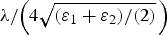${\lambda / {\left({4\sqrt {{{(\varepsilon _1+\varepsilon _2) } / (2)}} } \,\right)}}$ at $\lambda=0.8\, {\rm \mu m}$. Therefore, at the increase of number of nanodipoles, the amplitude of the scattered field at the short-wavelength resonance becomes comparable and further exceeds the amplitude of the long-wavelength resonance.

Fig. 13.

Characteristics of system of metal nanodipoles. Captions near the curves designate the number of nanodipoles in the system N, a = 0.03 µm, t = 0.01 µm, l = 0.25 µm, d = 0.1 µm.

Maximum of scattering diagram (Fig. 14) comes nearer to the direction of specular scattering.

Fig. 14.

Scattering pattern of system of metal nanodipoles; l = 0.25 µm, a = 0.03 µm, t = 0.01 µm, d = 0.1 µm. Wave is polarized along nanodipole, incidence angle –45°. Solid curves: $\lambda _r=$0.85 µm; dash curves: $\lambda _r=$ 2.5 µm. Curves: 1, single nanodipole; 2–5, nanodipoles; 3–10, nanodipoles.