

Total support to agriculture in the Organization for Economic Cooperation and Development (OECD) has remained steady at some $300 billion per year. Two-thirds of this amount is generated by instruments that support domestic prices, especially border protection, and one-third by direct fiscal subsidies. Domestic consumers mostly account for the former, while taxpayers incur the latter costs. Tariffs in agriculture are many times those applied to manufactures. The use of nontariff measures is as prolific in agriculture as it has become in manufacturing.
Understanding the political economy of agricultural support policies in OECD countries is important for those who pay the bill. Adoption of more efficient policy instruments to achieve agricultural objectives requires a good understanding of who is gaining from the status quo. It is also important in order to effectively negotiate in a multilateral forum, so that opposing sets of countries can identify policy packages that can mobilize domestic political support for reforms. De Gorter and Swinnen motivate the study of the political economy of agricultural policy as: “Understanding why governments do as they do allows one to analyze the policy formation process and alter incentive constraints through institutional reform in order to achieve desired policy outcomes.”1
de Gorter and Swinnen 2002, 1903.
The approach is based on the notion that governments trade off their governmental interests with the costs that their policies impose on society. Thus lobbying by special interests is intrinsic to the theory. While previous empirical studies find associations between special interests and agricultural protection, they lack the discipline imposed by theory on their empirical models. A primary objective of this article is to undertake a theoretically motivated empirical analysis of agricultural protection. We employ the Grossman-Helpman political economy model to investigate whether agricultural protection is a consequence of political campaign contributions.2
Grossman and Helpman 1994.
See Eicher and Osang 2002; Gawande and Bandyopadhyay 2000; Goldberg and Maggi 1999; Mitra, Thomakos, and Ulubasoglu 2002; and McCalman 2004. See also the survey by Gawande and Krishna 2003.
We go beyond previous empirical studies of the Grossman-Helpman model as well. We would expect a government that is influenced by contributions to trade off consumer welfare loss for contribution dollars on an about equal basis. However, previous studies indicate that the U.S. government is actually a welfare maximizer and places almost negligible weight on contributions. This article suggests a novel resolution for that puzzle. We show that it is the consequence of taking a feature of the theory all too literally. Doing away with the “unitary” government assumption and introducing policy uncertainty, that is, making the model more real worldlike, rids the paradox.
The article proceeds as follows. The first section briefly surveys the literature. It emphasizes the difference between the reduced form methods traditionally used in the agriculture protection literature and the structural method implemented in this article. In the second section the Grossman-Helpman model is introduced and its main predictions stated and described. The data are described in the third section. The data are new and theoretically appropriate for testing the model. In the fourth section the model's prediction is tested and the results analyzed. A puzzle posed by this and previous empirical work in this area is resolved. The final section concludes.
The First-Generation Literature
A number of authors have advanced extensions of the pressure group model building on a combination of the Olson-Stigler-Downs model to explain agricultural policies around the world.4
See Olson 1965; Stigler 1971; see also de Gorter and Tsur 1991. De Gorter and Swinnen 2002 provide the most up-to-date survey of this literature.
Olper 1998.
See Honma 1993; and Anderson and Hayami 1986. These findings also support the hypothesis in Anderson 1992 that contraction of the agricultural sector reduces consumers' resistance to agricultural protection and, by causing greater concentration, encourages political lobbying by farmers.
While this “first generation” of empirical studies conveys the message about the endogeneity of protection in agriculture, the empirical specifications they employ are ad hoc, with tenuous links to underlying theory. While this research finds strong associations of agricultural price distortions with some variables, the reduced form models cannot distinguish between competing theories. What theory are the results informing? Which theory should serve as the lens for best viewing the world of agricultural protection? This article is motivated by the need in the literature to begin second-generation work that is more theory-based and less ad hoc than these pioneering studies. The Grossman-Helpman model has the potential to become the dominant theoretical paradigm in the international economics literature as it offers a consistent and rigorous framework that integrates a number of the economic and political variables that motivated the first generation political economy models (and rejects others). Because this model is inspired by the political system prevalent in the United States, it is particularly well suited to be applied to U.S. agricultural protection.
This article thus departs in two important ways from previous empirical work. First, we employ a structural approach, where the empirical model is tightly linked with the theory. Second, rather than employing approximate measures of protection, we use ad valorem equivalents of protective instruments, just as the theory demands it.7
Traditionally, protection is measured by the nominal protection coefficient (NPC), which measures the difference between world and domestic prices as a result of the protection support, or the effective protection coefficient (EPC), which measures the amount by which protection raises value added, or the producer subsidy equivalent (PSE)/consumer subsidy equivalent (CSE), which measures the monetary benefit to producers/consumers as a percentage of production value in the absence of protection. We use ad valorem equivalents of tariffs and NTMs, which are more appropriate for the theory.
The Grossman-Helpman Model
The Grossman-Helpman general equilibrium theory of how trade policy responds to lobbying contributions delivers a precise prediction about the cross-sectional structure of tariffs and subsidies.8
Grossman and Helpman 1994.
Authors' observations from perusing a number of congressional profiles between 1980 and 2000 comprehensively summarized by Congressional Quarterly in their Politics in America volumes.
A unitary government is assumed to maximize a weighted sum of welfare (W) and lobbying contributions (C):

where a is the weight the government puts on a dollar of welfare relative to a dollar of contributions.10
While the political science literature has debated and gone beyond unitary government theories, formally complete models with more sophisticated forms of government are rare. The unitary government construct may be at the heart of why quantitative implications of empirical studies of the Grossman-Helpman model make the government out to be welfare maximizers even though this is inconsistent with the data. We return to this issue in the discussion of the empirical results, and offer a resolution that features congressional decision making.
First, consider producers of good i that compete with imports. An ad valorem import tariff ti on good i raises its price pi above the world market price piW. Revenues from the tariff are redistributed on a lump-sum basis to individuals in the economy. These individuals differ only in their ownership of sector-specific factors. Each individual owns capital that is specific to the production of one good. The supply of any sector-specific capital is limited, hence the rewards to specific capital used to produce good i increase with pi. This provides owners of sector-specific capital in any import-competing sector an incentive to politically organize and lobby the government for a tariff.11
Cross-commodity linkages are absent from the model, so that organized producers lobby only for protection to their good, not against protection on other goods. Consumers are the only group hurt by the tariffs. The relatively small input-output coefficients among the set of agricultural goods indicates that this assumption is well worth making for agricultural goods, and simplifies the model considerably. Cross-commodity linkages can be theoretically accommodated but introducing competition among lobbies makes the predictions less simple. Lopez 2001 studies cross-commodity linkages using a reduced form approach.
Now consider producers of good i that export to the rest of the world. An ad valorem export subsidy si on good i raises its price pi above the world market price piW. The costs of the subsidy are collected on a lump-sum basis from individuals in the economy. Symmetric to the import-competing case, owners of sector-specific capital in exporting sectors have an incentive to politically organize and lobby the government for a subsidy.
Suppose that sector i is an import-competing sector (the analysis for an exporting sector is symmetric). The lobby representing import-competing producers of good i presents government a menu that indicates the monetary contribution the lobby promises to make for each and every possible tariff ti.12
Formally, the menu is the set of contributions {Ci(tij),j = 1,…,∞} that maps each and every possible tariff for good i into a dollar contribution.
In this example, the single lobby gets to keep any and all surplus (the aggregate change in the welfare of each member net of contributions). When there is more than one lobby, due to the competition from other lobbies, they may be forced to collectively contribute beyond the welfare loss to the government. In that case, the government extracts part of that surplus. See Grossman and Helpman 1994, sec. 4.
We proceed by making the simplifying assumption that the politically organized population is a negligible fraction of the country's total population. The assumption is approximately satisfied for the U.S. agriculture sector that we empirically consider in this article. The corresponding predictions without this assumption are provided in accompanying footnotes. The assumption simplifies the main testable implication of the model in a manner that has both intuitive and empirical appeal. With the contribution schedules of the organized sectors in hand, the government sets equilibrium tariffs and subsidies that satisfy the following equations:14
In order to formally derive equation (2) it is easiest to use the Goldberg-Maggi bargaining game approach. Consider an import-competing sector i. The equilibrium tariff in sector i results from the maximization of the joint government-lobby (net) welfare function G + Wi − Ci where Wi − Ci is the welfare of lobby i net of its contributions. When the proportion of organized specific factor owners (in all sectors) is negligible in the population, the welfare of lobby i is simply the profits in sector i, or πi. Profit in sector i is a function of the sector i tariff ti. The joint government-lobby (in sector i) welfare is aW + Wi, where W the country's welfare (W is the sum of economy-wide wage income, profits, tariff revenue, and consumer surplus—the latter three being functions of tariffs). Applying the first order condition for a maximum to the joint net welfare, and noting that the lobbies in other sectors are too small to influence tariffs outside their own sectors, determines the optimal political-economic tariff in sector i as the first equation in (2). A symmetric derivation for exporting sectors determines the optimal export subsidy according to the second equation in (2).

In equation (2) ti is the ad valorem tariff on imports of good i and si is the ad valorem subsidy on good i in political equilibrium. Ii is an indicator variable that equals one if producers in sector i are politically organized into a (import-competing or exporting) lobby; a > 0 is the government preference parameter; ziM = yi /mi is the equilibrium ratio of domestic output to imports; and eiM is the absolute elasticity of import demand.15
Thus the logic of Ramsey pricing applies. If the demand for a good is uniformly less elastic than that for another good, the optimal tax rate is higher for the first good because of the lower deadweight loss from taxing it rather than the second good. If the first good is totally inelastic, there is no deadweight loss from taxing it, and the first best can be reached by taxing just this good.
The right-hand side of equation (2) indicates that protection to organized sectors is given according to their z/e ratios. Because the deadweight loss from protection (such as subsidies) increases with the absolute import demand (export supply) elasticities, the tariff (subsidy) varies inversely with elasticities, all else equal. The numerator of z, that is, output, formalizes the notion of the stakes from protection and subsidies. Thus contributions, and consequently protection/subsidies, vary directly with output. Finally, the lower the denominator of z (imports or exports), the lower the social cost that a tariff or subsidy imposes on the population, making the government more amenable to distorting prices in those sectors.16
The corresponding expressions without making the assumption that the number of lobby members are a negligible fraction of the population are:

The new parameter α is the fraction of the population organized into lobbies, and it measures the extent of opposition to protection. The first component on the right-hand side of equation (2) indicates that negative protection to unorganized industries is given according to their z/e ratios. This is because domestic consumers of that good (other than producers of the good) oppose protecting or subsidizing it because that raises the domestic price of the good. To the extent such consumers are politically organized they will lobby against protecting or subsidizing it. This component is less relevant for agricultural goods for the reason that if only a negligible fraction of consumers of agricultural goods were organized into lobbies (α = 0), there would be no organized opposition to protecting any sector, only organized support for protecting a lobby's own sector. Since the proportion of income spent on food is small in advanced countries, there is little if any counterlobbying by end consumers. Firms in food processing that use agricultural goods as intermediate inputs, who would normally oppose protection to agriculture, have chosen instead to lobby the government for protection to their sector. Mitra, Thomakos, and Ulubasoglu 2002 pay careful attention to issues relating to the estimation of the parameters a and α, and discuss how one interacts with the other.
Equation (2) presents a precise and testable implication about the cross-sector pattern of protection and subsidies, and it forms the basis for testing the Grossman-Helpman model. The tightness of the theoretical prediction makes it possible to measure the key political economy parameter a. The qualitative test of the model is that the coefficient on (Ii × zi /ei) is positive. Inverting the coefficient yields an estimate of a. The quantitative test of the model is whether these estimates of a are reasonable.
Empirical testing of the Grossman-Helpman model using nontariff barrier (NTB) data from the 1980s in U.S. manufacturing has been undertaken in two studies, by Gawande and Bandyopadhyay, and Goldberg and Maggi.17
Because U.S tariff reductions were the subject of multilateral reductions in the Kennedy and Tokyo Rounds, while the Grossman-Helpman model is one of unilateral protection, NTBs are more appropriate for testing the model. NTBs are measured as coverage ratios, that is, the percentage of imports covered by such barriers. Both studies qualitatively affirm the Grossman-Helpman model prediction. They find that protection increases with the inverse import-to-output ratio in politically organized industries (as measured by existence of political action committees or PACs).18Gardner 1987 is prescient about the Grossman-Helpman model's key features. In Gardner's model government maximizes the weighted sum of buyer's surplus (B) and producer's rents (R), B + θR. In turn, B and R are functions of farm output quantities. Efficient redistribution using production controls in this framework requires choosing quantities of farm products to maximize W. Unlike Grossman and Helpman, who adopt a formal model of the lobbying process and, as a result, are able to provide micro-foundations for their objective function, Gardner does not provide micro-foundations for W. He employs the “majority generating function” in Peltzman 1976 as the argument for using this type of objective function. He attributes the same forces that determine lobbying effectiveness as determining the value of the parameter θ. Gardner measures these forces for seventeen farm commodity by the number of producers, their geographical dispersion, the stakes from redistribution (output per farm), and the stability of the industry (variability of production patterns). He also estimates (long-run) demand and supply elasticities for those commodities. Pooling data across the seventeen commodities over the period 1912–80 yields a sample of 1,124 observations for Gardner's empirical analysis. The dependent variables are variants of the nominal protection coefficient. Gardner finds that the lower (greater) the (inverse) demand elasticity, the greater the level of intervention, that is, the higher the price relative to its nondistorted price. This is a confirmation of the Grossman-Helpman intuition that it is most efficient to tax commodities with the lowest price elasticities of demand and is the basis for Gardner's conclusion that interventions in U.S. agriculture have been efficient.
The empirical work of Mitra, Thomakos, and Ulubasoglu, and McCalman are notable for taking the theory to data outside the United States. While they affirm the model's prediction, they too find an implausibly high implied value of the government preference parameter a. The governments in Turkey and Australia19
attach more than fifty times as much weight on aggregate welfare as on contributions. This is grossly inconsistent with large deadweight losses that protection imposes on consumers as a number of U.S. case studies of protection demonstrate.20See, for example, Hufbauer, Berliner, and Elliott 1986; and de Melo and Tarr 1990. Gawande and Krishna's 2003 survey draws attention to this puzzle.
Agricultural data allow us to add new features to the empirical testing of the Grossman-Helpman model and thus significantly differentiate this study from the studies cited above and other forthcoming works. We are able to incorporate the use of subsidies into the model because they are pervasive in agriculture but rare in U.S. manufacturing. The pooling of both equations in (2) into one model is a unique feature of this article. We also consider the two equations separately. We estimate three cross-sectional econometric models based on stochastic versions of equation (2). The first model is given by the two-equation set:

In equation (3) εi is an identically independently distributed normal homoskedastic error term, which specifies the data generating process for the dependent variables. This model is estimated for the full sample of imported and exported goods. The model may be written with both equations stacked into a single equation with the terms redefined as:

where gi = ti and zi /ei = ziM/eiM if i is an imported good, and gi = si and zi /ei = ziX/eiX if i is an exported good. Data on protection and subsidies from 1998 are used to estimate this model across a cross-section of agricultural goods. The parameter of interest a is recovered as the inverse of the estimate of the coefficient β1.
Concern about the endogeneity of the regressor compels using the appropriate methodology. Quite clearly, import penetration (inverse of zM) is influenced by protection and the export-to-output ratio (inverse of zX) is influenced by subsidies. Further, which sectors are capable of organizing politically is also influenced in part by their expectation of the degree to which they will benefit from tariffs and subsidies. Thus the regressor Ii. zi /ei is a nonlinear transformation (here product) of two endogenous variables and is therefore itself endogenous. In order to estimate the coefficient β1 consistently we construct exogenous variables capable of instrumenting the component endogenous variables, and then use the method of Kelejian to instrument the composite regressor.21
Kelejian 1971.
Constructing instruments for the agricultural data is a nontrivial task due to paucity of data on variables that are truly exogenous. Testing the exogeneity of instruments is thus necessary. Even if instruments pass the test of exogeneity, it is prudent to investigate whether the instruments are “weakly” related to the endogenous regressor. If so, then it seriously affects inferences that may be made from small samples. An important literature has grown around this subject in recent years in response to strong concerns about the endogeneity problem in natural experiments.22
These studies and others indicate that the first-stage F-statistic may be used to assess whether a weak instrument problem exists. If a weak instrument problem exists, the popularly used two-stage least squares (2SLS) estimator can suffer a possibly intolerable level of bias. On the other hand, the limited information likelihood estimator (LIML) is a better-quality estimator and is more robust to the weak instrument problem. We report both the 2SLS and LIML results.23In addition to equation (4) we also estimate two models for separate samples of imported goods and exported goods. Protection is modeled in the imported goods sample as

and subsidies are modeled in the exported goods sample as

Whereas in equation (4) it is assumed that government's policy preferences are constant regardless of whether their decision is about protection or about subsidies, equations (5) and (6) allow flexibility in this regard.
Data
Protection
The data on protection and subsidies we use are not only comprehensive in the range of instruments they cover but are measured in a manner that fit the theoretical requirement of the model.24
We are grateful to Marcelo Olarreaga for access to this and other data that were constructed as part of the World Bank's project on trade restrictiveness.
Kee, Nicita, and Olarreaga 2004b.
Core NTMs include quantitative restrictions, price control measures, monopolistic measures and technical regulations corresponding to codes 6000, 8000, 7000, and 8100 in the UNCTAD TRAINS database, which is the source of the NTB indicators.
The method in Leamer 1990 is as follows. First, imports are predicted using factor endowments. Then the impact of NTBs on imports is measured as deviations of imports, in the presence of NTMs, from these predicted values. Finally, this quantity impact of NTMs on imports is converted into a price equivalent (or AVE) by using the import demand elasticities estimated in Kee, Nicita, and Olarreaga 2004a.
The second is an all-encompassing measure of protection, overall protection, which is the sum of all three possible sources of protection: tariffs, NTMs and domestic subsidies in agriculture.28
The source of the dollar value of agriculture domestic subsidies is Hoekman, Ng, and Olarreaga 2004, obtained from WTO members' notifications during 1999. The method of computing the AVE of domestic support is to treat them as NTMs and apply the same method as for core NTMs. Production subsidies vary widely in their uses and aims. They include direct payments to producers (such as deficiency payments), input subsidies (on irrigation water, for example), policies that distort market prices (market price supports), and interest subsidies on commodity loan programs. Also included in these measures are the “boxed” policies demarcated in the Uruguay Round. These include direct payments and price support benefits that directly influence production (“amber box”), payments tied to limits on production (“blue box” policies), research, domestic food aid, environmental programs, and certain crop insurance and income safety net programs (“green box” policies).
The third is a complete tariff measure, all tariff, which combines ad valorem tariffs with (ad valorem equivalents of) specific tariffs.29
The main source of the ad valorem tariff data is the WTO Integrated Data Base (IDB).
Specific (dollar/unit) tariffs can be converted to their ad valorem equivalents by dividing the specific tariff by the unit value of the imported product. The International Trade Commission (ITC) provides the data to accomplish this at the tariff line level.
The subsidy measures are taken from Hoekman, Ng, and Olarreaga.30
Hoekman, Ng, and Olarreaga 2004.
The range of included production subsidy measures can influence imports as well as exports—production subsidies can curtail imports (by increasing domestic production) or promote exports (by lowering production costs). For goods with one-way trade (goods that are purely exported or imported), it is clear what the subsidies achieve. For goods with two-way trade, we solve the problem by replicating them in the sample—once for imports, and once for exports. Protection data are used only with the imports sub-sample, while subsidy data are used only with the exports subsample.
Descriptive statistics for three samples: (1) imported goods, (2) exported goods, (3) M and X goods

Trade and Output
The U.S. Department of Agriculture's online Production, Supply, and Distribution (PSD) database (USDA 2002)32
Available at 〈http://www.fas.usda.gov/psd/complete_files/default.asp〉. Accessed 15 March 2006.
We use the following criteria to categorize commodities as pure import or pure export goods: if for any commodity zM > 30 (imports small relative to output) and zX < 30 then it is categorized as a pure export good; if for a commodity zX > 30 (exports small relative to output) and zM < 30 then it is categorized as a pure import good. In the data, in sectors where one ratio is greater than the cutoff of thirty, the other is considerably less than thirty, so that the cutoff clearly separates the exported commodities from import-competing ones.33
This applies to commodities with zero imports (so that zM is infinite), and zero exports (zX = ∞).
If both zX < 30 and zM < 30 then the sector is categorized as a two-way trade sector. In the sample, they are replicated, once as an import good for which zM is the relevant variable, and once as an export good for which zX is relevant. Thus, in the sample used to estimate equation (4), there are ninety-four observations, forty-one for imports and fifty-three for exports. Table 1 breaks down descriptive statistics for the three samples.
Another study by Kee, Nicita, and Olarreaga estimates U.S. import demand elasticities at the tariff line level using the gross domestic product (GDP) function approach.34
Kee, Nicita, and Olarreaga 2004a. See, for example, Kohli 1991 for the GDP function method. In this method imports are treated as inputs into domestic production, given exogenous world prices, productivity and endowments.
Fuller 1986. The idea behind this correction is to limit the influence of estimates that are large and also have large standard errors. Without the correction, these large estimates would grossly overstate the true elasticity. The correction mutes their effect.
Lobbying
Agricultural PAC spending data for the three congressional election cycles between 1993–98 were downloaded from the Federal Election Commission (FEC) Web site.36
See www.fec.gov.
Mapping PACs into SIC-based agriculture-related sectors was done via a concordance constructed by Beaulieu and Magee 2004. In most cases many PACs mapped into one SIC code, so SIC level contributions are simply the aggregate of the mapped PACs. For one-to-many maps, political contributions from each PAC were fractionally assigned equally to each SIC code into which the PAC mapped. To check for consistency we compared our data with the data on the opensecrets.com Web site. For the few sectors in which opensecrets.com reports such information our data closely matched theirs. Accessed 15 March 2006.
It is instructive to examine some features of PAC spending data and assess whether they are in line with the Grossman-Helpman idea of money buying policy (as distinct from money buying mere access to policymakers).38
Gawande 2006 details the structure of lobbying in agriculture over the 1990–2000 period in the United States.
Food manufacturing PACs, forestry and nursery PACs, agriculture service PACs, and agriculture distribution PACs contributed more than did farm PACs.
Based on Herfindahl indices computed by Gawande 2006.
PAC money is clearly influential in agriculture. A study of the 1985 and 1990 voting during sugar legislations by Brooks, Cameron, and Carter finds that in the House and Senate both votes were responsive to sugar PAC contributions.41
Brooks, Cameron, and Carter 1998. Lopez 2001 also finds that PAC contributions influenced agricultural policies in other sectors.
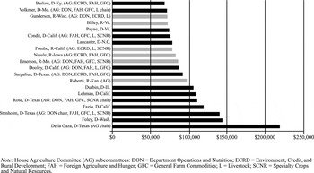
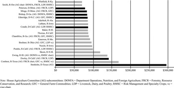
Two-thirds of agricultural PAC money went to House candidates and one-third to Senate candidates. Figure 1 indicates the top twenty recipients in the House of agriculture PAC contributions during the 1993–94 election cycle.42
The PAC data are in three relational data files: candidate information files (CN), PAC committee information files (CM), and files containing transactions between PACs and candidates (PAS). For each election cycle, aggregate contributions by each PAC to every candidate were computed from the PAS files, and then merged with the relevant cycle's CN files. Agriculture committee and subcommittee assignments for each Congress were obtained from Congressional Quarterly 1996–99. See Gawande 2006.
House members who made the top twenty who were not on the Agricultural Committee represented districts with influential agricultural constituents (California, Oklahoma, Virginia, Michigan). For example, Fazio's district (California District 3) was among the thirty leading districts by market value of agricultural products (1997 Census of Agriculture).

Top 20 House recipients of AG PAC money: 1993–94 election cycle

Top 20 House recipients of AG PAC money: 1997–98 election cycle
Instrumental Variables
Because the regressor is composed of the endogenous variables I and z we construct two exogenous variables from the agriculture census of 1997 that identify each of the endogenous variables. The first instrument, termed paymentconcentration, is a measure of geographic concentration and pressure. It is constructed using data on total government payments available for each state. Total government payment to a state is then distributed across the top four commodities produced in that state.44
These include payments for acreage reductions, commodity credit loans, payments for meeting environmental targets satchel wetlands, and so on.
Empirical Analysis
Results
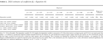
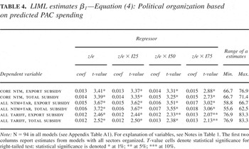
The first set of results we discuss are estimates of equation (4) using the sample of ninety-four observations in which both import-competing and exported goods are stacked. Each row in Table 2 contains estimates of β1 from seven specifications of equation (4). Each specification uses a different definition of political organization, Ii. Their purpose is two fold. First, contributions do not necessarily imply that a particular commodity is politically represented in the trade arena, the relevant policy domain for the Grossman-Helpman model. Agricultural producers have historically benefited from a basket of instruments such as acreage controls in addition to trade protection and subsidies.45
Goldstein 1989 provides an illuminating account of the evolution of agricultural institutions.
2SLS estimates of coefficient β1—Equation (4)

Each of the six rows in Table 2 defines the dependent variable differently. The first two rows use the (core ntm, subsidy) combination for the dependent variable, that is, for import-competing goods protection is measured as core ntms, while for exported goods subsidies are measured as export subsidies (row 1) or total subsidies (row 2). The next two rows use the (overall protection, subsidy) combination, and the final two rows use the (tariff, subsidy) combination. A diverse range of instruments is thus represented in Table 2, allowing for a more inclusive test of the Grossman-Helpman model than previous tests that have used data only on imports.
The forty-two models in Table 2 are estimated using Kelejian's two-stage least squares (2SLS) method (see above), using as instruments the variables paymentconcentration, Farmland, their squares and cross-products. In the first model in Table 2, 90 percent of the sample is organized. The variable Ii equals 1 if total PAC spending over the 1993–98 period for sector i is ranked above the bottom tenth percentile of the sample. T-values are reported next to the estimates of β1. Starred t-values denote statistical significance for 1-tailed test. The signs and statistical significance on the estimates affirm the Grossman-Helpman prediction across all models, even those with few (though influential) politically organized sectors. The positive and statistically significant estimates of β1 demonstrate that political organization increases agricultural protection to import competing sectors and subsidies to exporting sectors according to their z/e ratio. For commodities whose producers are politically organized, the greater the stakes from protection (high output) and the lower the deadweight loss from protection (low imports, low e), the greater is the difference between domestic and world prices.
A change in z/e in an organized industry changes the level of protection/subsidy by β1 > 0. For example, the middle two rows of Table 2 indicate that an increase in the output-to-import or output-to-export ratio by 100 would increase the dependent variable in equation (4) by anywhere between 18 and 24 percent.46
In the cross section, due to wide disparities in the z/e ratios, differences of that magnitude are not uncommon.
A 1 percent change in the dependent variable in equation (4), g/(1 + g), translates into a (1 + g) percent raise in the ad valorem tariff or subsidy, g. At the sample mean of g = 0.082 (see Table 1), we obtain these estimates.
Quantitatively, the results echo a puzzling finding from previous examinations of the Grossman-Helpman model that used manufacturing data. Inverting the coefficient estimate yields estimates of the government preference parameter a. These implied estimates are skewed toward welfare. The last two columns of Table 2 indicate that, across the models, the implied estimates of a lies between 47.6 and 62.5 when the dependent variable is the (core ntm, export subsidy/total subsidy) combination, between 41.7 and 55.6 with the (overall protection, export subsidy/total subsidy) combination, and between 83.3 and 100 with the (tariff, export subsidy/total subsidy) combination. They show that government places far greater weight on a dollar of welfare, at least forty times as much, as on a dollar contributed politically.
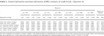
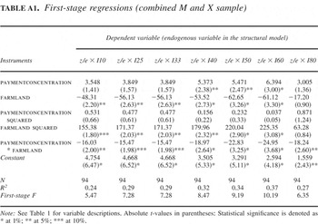
The first robustness test we undertake is with respect to the validity of the five instruments used in the first stage. The set of instruments pass the Sargan test of overidentification, that is, the instruments prove to be exogenous and uncorrelated with the errors in the structural equation. But that in itself is not sufficient to guarantee reliable inferences in small samples if instruments are “weak.” Intuitively, when instruments are only weakly related to the endogenous regressor, then t-tests based on conventional asymptotic approximations can be quite inaccurate. Stock and Yogo show that, with five instruments, the first-stage F-statistic must be greater than 6.40 in order for the bias of the 2SLS estimator relative to the (large sample) bias of the OLS estimator to be lower than 20 percent.48
Stock and Yogo 2005.
Limited information maximum information (LIML) estimates of coefficient β1—Equation (4)

A second set of robustness tests is based upon new political organization variables constructed by predicting PAC spending from a linear regression with the output-to-import or output-to-export ratio z as the regressor. This method yields better measures of trade-related lobbying than using the raw lobbying data. Table 4 presents results using these measures. The variable I is now based on percentile cutoffs using the predicted value of PAC spending. The results prove robust to these new variables. The last two columns of Table 4 indicate somewhat larger implied estimates of a when the dependent variable is the (core ntm, export subsidy/total subsidy) or (overall protection, export subsidy/total subsidy) and a somewhat smaller estimate with the (tariff, export subsidy/total subsidy) combination. They show that government places at least 55.6 times (and as much as 83.3) as much weight on a dollar of welfare as on a dollar of contributions.
LIML estimates β1—Equation (4): Political organization based on predicted PAC spending

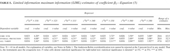
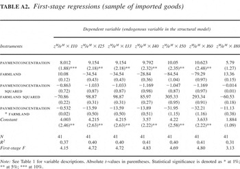
Does splitting the sample separately into import-competing and exporting goods alter the magnitudes of the a estimates? This question is addressed in the third set of robustness tests we undertake. Table 5 presents LIML estimates from the imports samples, where the dependent variables are measures of protection. The first-stage F-statistics (see Table A2 in the Appendix) lie between 4 and 5 for the imports sample, so that LIML proves to be the more robust estimator for this sample. The last two columns indicate that the preference parameter a lies between 20.8 (Overall protection model) and 62.5 (all-tariff model) across the three measures and the variety of I measures—a relatively smaller range of estimates than with the full sample, but not significantly so.
Limited information maximum information (LIML) estimates of coefficient β2—Equation (5)

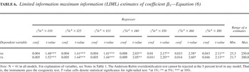
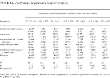
Table 6 presents LIML estimates from the exports sample, where the dependent variables are the two subsidy measures. The first-stage F-statistics (see Table A3 in the Appendix) range from a low of 0.54 (model with I80) to a high of 5.27 (model with I60). The LIML estimator is therefore robust to the weak instrument problem for only models with intermediate measures of political organization. Therefore the lower limit of the a estimates (which come from the model with I80) are quite unreliable. It would be safest to infer that a exceeds 100 (and is less than 250) from the subsidy data. The results are therefore quite robust to differential rates of tradeoff between lobbying contributions and welfare that may characterize U.S. government preferences across policy instruments.
Limited information maximum information (LIML) estimates of coefficient β3—Equation (6)

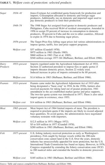
The main implication from the estimates of the preference parameter a in Tables 2, 3, 4, 5, and 6 is that the observed values of z/e and their interactions with I can only lead to the observed levels of NTB protection and subsidies if government puts great weight on welfare. That is, the U.S. government is approximately a welfare maximizer. But welfare maximization would lead to free trade, and trade in agriculture is by no means free! The deadweight losses from protection are considerable. Table 7 compiled from Hufbauer, Elliott, and Schott, indicates the extent of those losses from protection in U.S. agricultural products.49
Hufbauer, Berliner, and Elliott 1986.
Friedman 2003 estimates are based on the following calculation: in 1995 total receipts for the grain crops were in the $40 to $50 billion range. Approximately 41.9 percent of these receipts come from direct or indirect government support, implying total transfers in the $17 to $21 billion range. The deadweight losses various studies have cited for different commodity programs are in the range of 10 to 30 percent of transfer payments, which is $1.7 to $6.1 billion for the grains.
Welfare costs of protection: selected products

First-stage regressions (combined M and X sample)

First-stage regressions (sample of imported goods)

First-stage regressions (export sample)

How is one to resolve this paradoxical finding about a? We start by exploring the idea that the large estimates of a are a consequence of the model's assumption that contributions are far larger in magnitude than they actually are. As described previously, in order to induce government to implement a policy, the change in contributions from any lobby due to a small change in policy must, at the margin, compensate the government an amount equal to a times the loss in consumer welfare plus (in the case of a single lobby, and more if there is lobbying competition).51
Mathematically this is immediate from differentiating equation (1) with respect to the vector of prices p. See note 13.
Reconciling the Results: Lobbying Under Policy Uncertainty
In order to resolve the puzzle, we amend the theory to make it capable of generating the real-world lobbying and protection data. A contribution of this article is to bring the model closer to legislative reality. The Grossman-Helpman model presumes government to be a singular entity with the power to supply protection with certainty. In reality the legislative process leading to protection is uncertain. First, contributions are made ex ante to the award of protection or subsidy. They are not, as in the Grossman-Helpman model, made on delivery of protection or subsidy. Second, lobbies make contributions to a number of political agents who, neither individually nor collectively, can guarantee a specific outcome, as the unitary government of Grossman-Helpman can. The legislative studies literature has rejected the “straw man” unitary government hypothesis. A voluminous literature in this area seeks to understand the complexities of the legislative process. Not only can a potential policy be stillborn as it fails in committee, in the chambers, or is vetoed by the executive, but even if it makes it through, its shape may be indelibly and unpredictably altered as it encounters gatekeepers, opportunists (“log-rollers”), and legislators with the power and influence to form deal-breaking coalitions at various stages of its journey. Legislative uncertainty is in fact the norm for trade policy owing to its essentially redistributive nature that creates gainers and losers. For example, the 1989 Trade Omnibus bill was characterized by logrolls, mark-ups, and an executive veto before a much milder and less protectionist form of legislation was passed by Congress.
Thus protection is for sale, but uncertainly, because lobbying contributions are made in advance of knowing the outcome.52
Specifically, unlike the GH model in which the government is promised a contribution Ctij by lobby i for every possible tariff tij, j = 1,…,∞, and collects from lobby i its promised contribution Cti* after delivering a particular policy ti*, in reality each lobby must make a contribution knowing only that a policy tij can be delivered only uncertainly. A specific policy here is a vector of tariffs and subsidies across all goods, where, under the assumption that a negligible proportion of the population is organized, each lobby is concerned about only that element of the vector pertaining to its own sector, that is, its own tariff/subsidy.
In order to understand this more formally, compare the maximization of the joint government-lobby i net welfare function under certainty about policy versus uncertainty. The former is given in n. 14 as G + Wi − Ci, where Wi − Ci is the welfare of lobby i net of its contributions. Under uncertainty, where the government can deliver a tariff ti with probability γ, the joint net welfare function becomes G + γWi − Ci, since ex ante to the policy lobby i can only maximize expected welfare. Applying the first order condition for a maximum to the joint net welfare under uncertainty now determines the optimal political-economic tariff in sector i as the first equation in equation (3), and the optimal export subsidy as to the second part in equation (3).

The parameter γ sharply differentiates the equilibrium in equation (7) from that in equation (2). Under uncertainty, the political economy parameter a is retrieved as γ/β1 from the econometric model (3). Thus if γ = 0.10, the estimate of parameter a drops to between 4 and 6, or one-tenth of the estimate under certainty (using LIML estimates in the first two rows of Table 2). Bringing uncertainty about government's ability to deliver policy into the Grossman-Helpman model thus brings many results into line with reasonable prior beliefs based on facts about (low) contributions and (large) deadweight losses.
An intuitive approach to understand the mechanism that is altered by introducing policy uncertainty is to consider what happens to lobbying contributions. Consider the instructive case of a single lobby which exists, say, in sector 1. As described in the second section of this article, under certainty the lobby presents the government with a menu of contributions in which it promises to pay the government a times the deadweight loss (DWL) for every possible tariff. This clearly overstates actual contributions in the real world. Under uncertainty, the lobby pays the government (ex ante to the policy) an amount equal to a times γ times the deadweight loss (DWL) from the expected tariff. For example, if contributors viewed the probability of protection to be 10 percent, then contributions in the same model would equal a time expected deadweight loss, or a × 0.1 × DWL. The government receives far less in contributions than the deadweight losses its policies impose, because the contributions come ex ante to the policy. The “case of the missing lobbying” thus stands resolved.54
We can approach PAC spending formally. Consider the expression that approximates DWL in a sector. See, for example, Vousden, 1990:

where y is output. Substituting for t/(1 + t) from (2) yields

In the single-lobby case described above, the numerator on the left hand side equals PAC spending in the Grossman-Helpman model, or

Thus PAC spending by the industry's lobby as a fraction of industry output is predicted by the Grossman-Helpman model to be proportional to z/e, the factor of proportionality being (approximately) 0.5/a. With legislative uncertainty, the mapping from DWL into z/e is modified as protection (an therefore) DWL becomes probabilistic in the eyes of the lobby. Thus, if E(DWL) = γ × DWL, then

Under uncertainty the model predicts that PAC spending as a fraction of output is proportional to (z/e) the factor of proportionality being (approximately) 0.5 × γ/a.
Furthermore, the actual level of protection to sector 1 is lower because contributions are lower. If contributions are thought of as being determined within the unitary government framework of Grossman and Helpman, when in reality they are determined ex ante to a policy that a divided government can only deliver with uncertainty, then the level of protection will be (erroneously) predicted to be greater than it is in reality. The result is that the unitary government model leads to the conclusion that the low tariffs are due to a welfare-supporting government, when in reality it is a self-interested government that delivers tariffs in response to (lower) contributions under uncertainty.
On the supply side, why should a mulitlayered government agree to provide redistributive policies to a handful of winners at a low price? To this question, we provide an intuitive answer but await more formal explanations from future research. In the real world, to maximize the impact of their limited budgets (determined by the lobby on their assessment of the policy uncertainty parameter γ) agricultural lobbies strategically target a handful of politicians, such as ranking members of the House and Senate agriculture committees. Members of Congress on the agricultural committee are more than willing to bear their share of the deadweight loss from distortionary agricultural policy. It is clear from Figures 1 and 2 that representatives of agricultural constituencies vie for membership on agricultural committees so that not only are they able to influence policy to suit their constituencies but they are also lobbied in the process. Formal extensions of the Grossman-Helpman theory in this direction should recognize the paramount importance of committees in legislative decisions.55
See, for example, Fenno 1973; Grier and Munger 1991; Weingast and Marshall 1988; and Grossman and Helpman 2002.
Once the issue leaves the committee for the floor, why should other members of Congress that bear the deadweight loss, but are not compensated by lobbies, care to vote for the distortionary policy? Distributional models of legislative organization recognize that legislators are a heterogeneous group and care differentially about different issues.56
Mutual gains make it almost necessary to trade votes across issues. In this view, agriculture committee members are supported in exchange for their reciprocal support on issues on which the agriculture committee members bear their portion of deadweight loss without being compensated. Proof of vote trading in the U.S. Congress and its quantitative importance is demonstrated by Stratmann, who finds that vote trading among farm interests is widespread, and that such logrolling coalitions exhibited a strong degree of stability.57 His analysis of logrolling during voting on the 1985 farm bill shows strong evidence that legislators traded votes.58Stratmann 1992.
It is appropriate at this stage to consider whether competing views about lobbying might not be more relevant than the Grossman-Helpman view of lobbying as exchange. An alternate view is one where lobbying spending provides access to politicians. This opens the door for lobbies to provide politicians with information that benefits them and simultaneously implies policies that benefit the lobbyist.59
Hansen discusses milestones in agricultural policymaking during the twentieth century that he posits were due to informational lobbying.60Hansen 1991 finds that in the 1950s and 1960s farm policymakers dropped the American Farm Bureau Federation (AFBF) from its dominant position in agricultural politics. AFBF had been agriculture's leviathan for a generation. In the 1960s and the 1970s, commodity organizations replaced the position previously occupied by the AFBF. Also, in the 1960s and the 1970s, farm policymakers paid less and less attention to the advice of farm lobbies. In the 1970s and 1980s, this was reversed, and they scarcely paid attention to the advice of consumer lobby. In sum, during those forty years, Congress reallocated access within the farm lobby, and Congress restricted access for the farm lobby but it denied access to the consumer lobby. Hansen's theory of these changes in access is developed around (1) competitive advantage in a lobby's ability to deliver better information to politicians than their rival groups, and (2) recurrence of issues around which a lobby makes its case to the politicians. Hence, politicians grant access to lobbies on the basis of their informational advantage over other lobbies, and also the permanence of the issues and positions conveyed by the lobbies.
Evidence on the effectiveness of informational lobbying in agriculture is, at best, feeble. Wright finds only weak evidence of informational lobbying of the House Agriculture Committee, the most influential policymaking committee in agriculture.61
Wright 1990.
Parker and Parker 1998.
Therefore, we do not see a role for informational lobbying in agriculture, at least over the short duration of a decade. Our experiment is different from Hansen's, who considers a longer period in history during which there were points in time when Congress sought new information from lobbies. At those threshold points, informational lobbying may have led to marked shifts in how Congress began to view agricultural policy. On a continuing basis over the 1991–2000 period we see little role for new information. Our view is thus that agricultural PACs contributions are more in the spirit of exchange or payments in political markets for protection, as Grossman and Helpman posit. With the “paradox of the high a” resolved, the amended and extended Grossman-Helpman model presents an emerging new paradigm in the literature on the political economy of trade policy.
Conclusion
The theoretical lens of the Grossman-Helpman model is used in this article to investigate the political economy of U.S. agricultural protection and subsidies. Because the theory delivers clear empirical predictions about the structure of protection, empirical estimation of the determinants of protection and subsidies may be tightly linked to theory. The model thus encourages structural econometric estimation of the political economic determinants of protection and subsidies. This is in contrast to the ad hoc specifications in previous empirical, but, not any less important, exploratory work in this area. This is the first attempt at applying this model to study agricultural protection. Estimates from the model strongly affirm the qualitative implications of the Grossman-Helpman model. They clearly establish that interest-group money bends agricultural policy in the United States.
Quantitatively, accepting the theory literally leads to the inferences that the U.S. government is a welfare maximizer. This is inconsistent with the large estimates of deadweight losses from distortionary policy in agriculture, and the small amount of money contributions that are able to “buy” that policy. We show that the puzzle is resolved by extending the model to allow uncertainty about the ability of politicians to deliver policy combined with the fact that contributions are made ex ante to the policy. It makes common sense that lobbies, who must determine how much to contribute under uncertainty about the “product” they wish to purchase, contribute much less than in a world where there is no uncertainty.63
Perhaps it is this uncertainty that forces them to try to gain access to policymakers to use forms of persuasion that are less costly than quid pro quo money payments.
The results of the empirical estimation clearly reveal the government-business political nexus that underlies the equilibrium with agricultural protection. Making agricultural liberalizations the focus of the Doha Round has caused the negotiations to stumble. If this is a “crisis of multilateralism,”64
Martin 1992.
Comparatively, the persistence and near-universality of agricultural protection among the rich countries suggests that alternative political institutions may produce similar outcomes. Though the model is framed in terms of government trading off the welfare of its polity for lobbying contributions, it applies generally to governments who trade off welfare for considerations that improve their chances of being reelected. Thus the European Union (EU) governments are able to provide price supports to their farm lobbies and distribute those costs over a broad polity. Thus countries such as Argentina, once at the forefront of agricultural technology and productivity, now distort prices in a manner that erodes the sector's competitiveness. This article suggests that behind the institutional variation across high- and middle-income countries lie some basic similarities in the way governments are willing to make trade-offs. The main obstacle to multilateral liberalization perhaps has its source in the political economic mechanism described here, which makes governments resist even small changes to the status quo.
Our resolution of the missing lobbying paradox also raises questions. We close on the note that these may also be answered in future research. What are realistic values of the uncertainty parameter γ? Should this parameter be modeled as being different for different sectors?
Agricultural cases that have been awarded antidumping or countervailing duties, instances of barriers at the border under the guise of quality controls, and exclusions of agriculture from a free trade agreement may be used to investigate whether actual barriers to agricultural trade fluctuate enough to support a sizeable policy uncertainty parameter. This may also shed light on whether the committee and the legislature treats some subsectors more specially than others, and the reasons for such treatment. Finally, can structural models of policy uncertainty because of, for example, the existence of veto players66
be incorporated to generate realistic hypotheses of not only the structure of protection and subsidies but also about how such uncertainty conditions lobbying behavior?