1 Introduction
This paper describes measurements and analysis of the transversely forced shear layer dynamics of a swirling, premixed flame. Both reacting and non-reacting swirling jet flows exhibit a variety of unsteady features associated with underlying hydrodynamic instabilities. In particular, high swirl flows exhibit vortex breakdown above a critical swirl number, leading to a pocket of central recirculating flow (Faler & Leibovich Reference Faler and Leibovich1977; Wang & Rusak Reference Wang and Rusak1996; Rusak et al. Reference Rusak, Wang, Xu and Taylor2012). In these flows, the instantaneous centre of rotation of the swirling flow can precess around the geometric or time-average centre of rotation, a phenomenon known as the precessing vortex core (PVC).
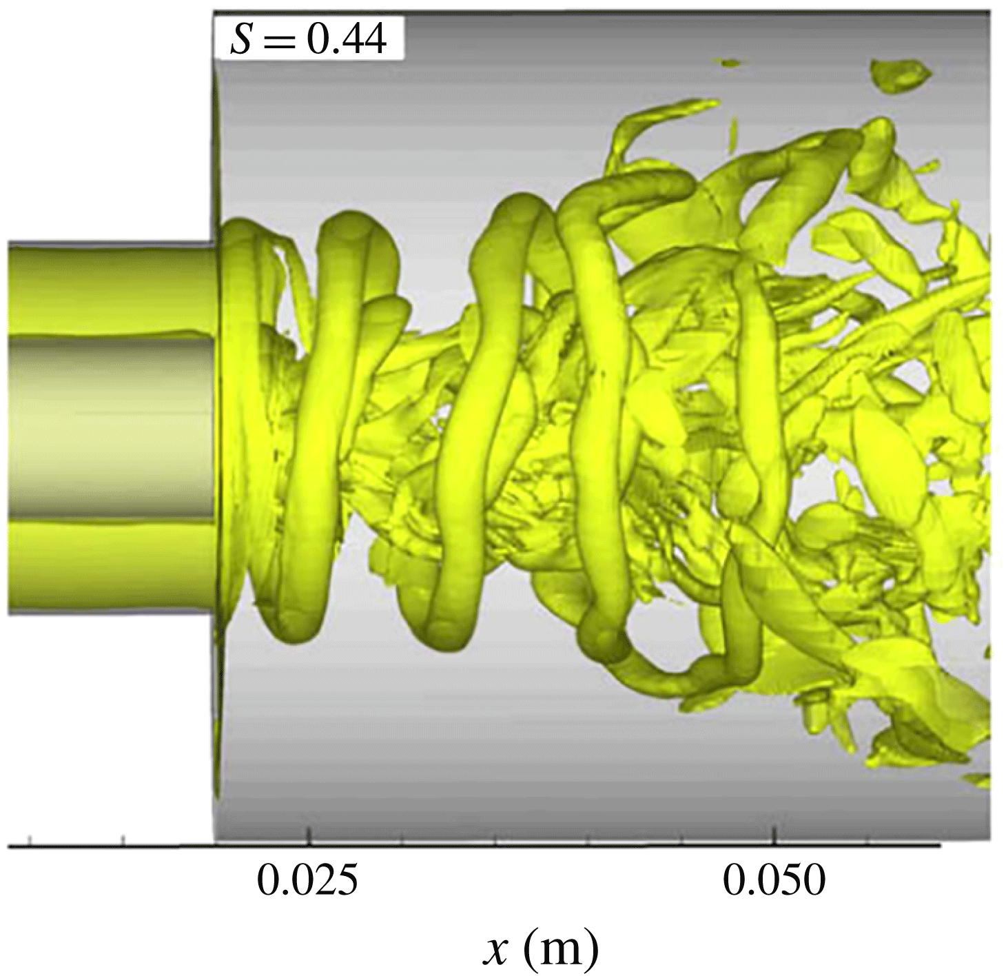
In addition to the substantial influence of vortex breakdown on both time-averaged and unsteady flow features, swirling flows generally contain free shear layers in both the radial and azimuthal direction. For example, flows with a centre body are quite common and have two separating shear layers which are subject to the Kelvin–Helmholtz instability, leading to the concentration of vorticity originating from the separating boundary layers into helical structures as illustrated in figure 1. The mechanism responsible for the occurrence of these helical structures is quite distinct from that of vortex breakdown and the PVC, although they are strongly coupled. There is an enormous literature on vortex precession and/or helical flow disturbances in swirl flows, for both non-reacting and combustion flows (Syred Reference Syred2006; Arndt et al.
Reference Arndt, Steinberg, Boxx, Meier, Aigner and Carter2010; Fanaca et al.
Reference Fanaca, Alemela, Hirsch and Sattelmayer2010; Day et al.
Reference Day, Tachibana, Bell, Lijewski, Beckner and Cheng2012; Steinberg et al.
Reference Steinberg, Boxx, Stöhr, Meier and Carter2012; Qadri, Mistry & Juniper Reference Qadri, Mistry and Juniper2013). Comprehensive reviews and reference lists are given by Syred (Reference Syred2006) and Huang & Yang (Reference Huang and Yang2009). The helical disturbance found in the flow field, described by the azimuthal mode number,
 $m$
, depends strongly on the swirl number and flow profile; e.g. whether the flow features are ‘wake-like’ or ‘jet-like’ (Liang & Maxworthy Reference Liang and Maxworthy2005). For example, the experiment of Liang & Maxworthy (Reference Liang and Maxworthy2005) showed that a swirling jet without a centre body after vortex breakdown had a dominant counter-winding
 $|m|=1$
helical disturbance with a simultaneous but weaker counter-winding
 $|m|=2$
mode.
Iso-vorticity surface demonstrating the shear layer roll up into a helical mode in a swirling flow (Huang, Wang & Yang Reference Huang, Wang and Yang2006, reproduced with permission from the authors).

In order to fix some notation, we use the same conventions as Oberleithner, Paschereit & Wygnanski (Reference Oberleithner, Paschereit and Wygnanski2014) and denote a complex helical disturbance,
 $\hat{A}$
, indexed by the azimuthal mode number
 $m$
as a function of frequency,
 $\unicode[STIX]{x1D714}$
(defined to be positive), in a polar coordinate system
 $(r,\unicode[STIX]{x1D703},z)$
, as
 $$\begin{eqnarray}\hat{A}_{m}={\hat{C}}_{m}(r,z)\exp [\text{i}(\unicode[STIX]{x1D714}t-m\unicode[STIX]{x1D703}-kz)],\end{eqnarray}$$
where
 ${\hat{C}}_{m}$
is the complex coefficient, the hat denotes a complex number and
 $k$
is the axial wavenumber. The
 $m=0$
mode is axisymmetric while the
 $m>0$
and the
 $m<0$
modes denote counter-clockwise and clockwise rotations of iso-phase surfaces within an
 $r$
–
 $\unicode[STIX]{x1D703}$
plane. The mean swirl is counter-clockwise and positive
 $\unicode[STIX]{x1D703}$
is in the counter-clockwise direction, so that the
 $m>0$
and
 $m<0$
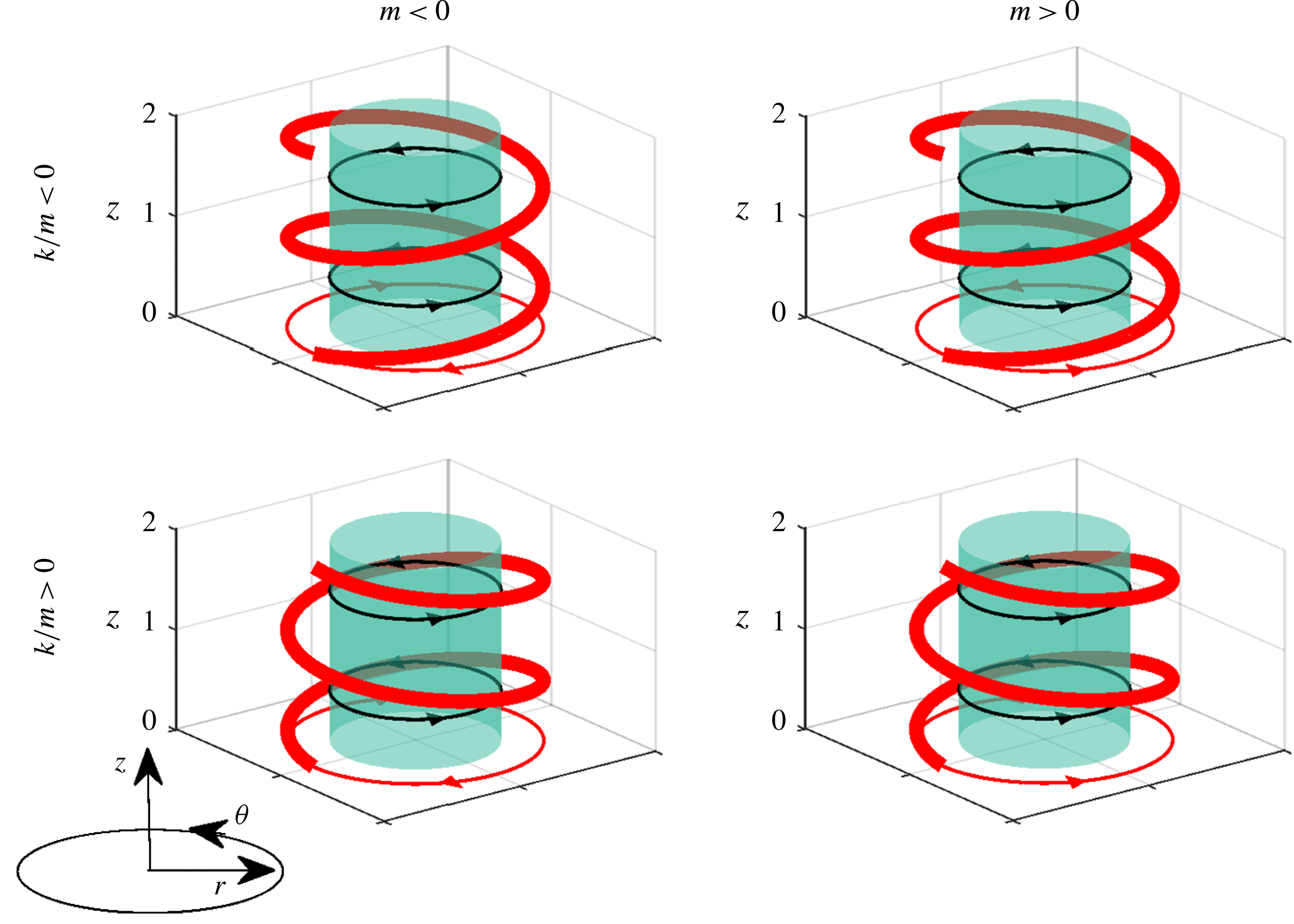
modes refer to co- and counter-rotating modes respectively. The co- and counter-winding terms refer to the direction the helix winds with respect to the mean swirl, as shown in figure 2. A co-winding direction is expressed as
 $k/m<0$
while a counter-winding disturbance is
 $k/m>0$
. The velocity measurements presented here denote the temporal Fourier transform of the fluctuating velocity vector,
 $\boldsymbol{u}^{\prime }(r,\unicode[STIX]{x1D703},z,t)$
(using the
 $\exp (\text{i}\unicode[STIX]{x1D714}t)$
convention) by
 $\hat{\boldsymbol{u}}^{\prime }(r,\unicode[STIX]{x1D703},z,\unicode[STIX]{x1D714})$
and decompose the complex velocity into azimuthal modes, indexed by
 $m$
:
 $$\begin{eqnarray}\hat{\boldsymbol{u}}^{\prime }(r,\unicode[STIX]{x1D703},z,\unicode[STIX]{x1D714})=\mathop{\sum }_{m=-\infty }^{\infty }\hat{\boldsymbol{B}}_{m}(r,z,\unicode[STIX]{x1D714})\text{e}^{-\text{i}m\unicode[STIX]{x1D703}},\end{eqnarray}$$
where
 $\hat{\boldsymbol{B}}_{m}$
is the complex coefficient of the helical mode
 $m$
containing the spatial amplitude of the mode and the spatial phase information including the
 $\exp (-\text{i}kz)$
term in (1.1).
Diagram demonstrating winding and rotation direction of helical
 $|m|=1$
iso-phase surface shown in red. Black arrows denote mean swirl direction, and red arrows denote rotation direction of iso-phase surface in
 $r$
–
 $\unicode[STIX]{x1D703}$
plane.

The particular focus of this study is on flows with external transverse forcing. The presence of transverse forcing on this naturally unstable flow both influences the natural instabilities, as well as amplifies disturbances that may not necessarily manifest themselves during natural oscillations. This occurs because swirling jet flows have a variety of different underlying modes with different spatio-temporal growth rates. For example, the axisymmetric
 $m=0$
shear layer mode is strongly excited in the presence of axial forcing, even in situations where the natural instability of the flow manifests itself as a strong helical disturbance (Lacarelle et al.
Reference Lacarelle, Faustmann, Greenblatt, Paschereit, Lehmann, Luchtenburg and Noack2009). Numerous observations of combustors undergoing axial thermoacoustic oscillations note the suppression of the strong helical structures in the flow in this case, as the forcing of the underlying axisymmetric mode is so strong (Lacarelle et al.
Reference Lacarelle, Faustmann, Greenblatt, Paschereit, Lehmann, Luchtenburg and Noack2009; Roy et al.
Reference Roy, Yi, Jiang, Gunaratne, Chterev, Emerson, Lieuwen, Caswell and Gord2017).
The motivation for the forced problem arises from the problem of combustion instabilities, which pose significant operability challenges in premixed combustors (Lieuwen Reference Lieuwen2012). These thermoacoustic instabilities act as a source of strong, narrowband acoustic forcing to the flow, with a spatial structure that is controlled by which natural acoustic mode is coupled to the oscillations (Steinberg, Arndt & Meier Reference Steinberg, Arndt and Meier2013; Rosa et al. Reference Rosa, Samarasinghe, Peluso, Quay and Santavicca2016). O’Connor, Acharya & Lieuwen (Reference O’Connor, Acharya and Lieuwen2015) recently reviewed transverse instabilities, and summarized key influences of the injector/nozzle location within a transverse acoustic field, the excitation of hydrodynamic instabilities by acoustic waves, and how the heat release responds to these disturbances.
A key feature of the transverse excitation problem relative to the axial one is the fact that it excites more spatial degrees of freedom of the underlying hydrodynamic modes. For example, axial instabilities often can be approximated by a nominally one-dimensional acoustic field, and excite dominantly axisymmetric vortical structures that distort the flame in an axisymmetric manner. In contrast, transverse instabilities are associated with multi-dimensional acoustic fields and excite three-dimensional, helical flow disturbances that subsequently disturb the flame. In addition, different nozzles/flames are located at different points in the travelling or standing wave structure in a transverse instability, and different hydrodynamic stability modes are preferentially excited at each location (Worth & Dawson Reference Worth and Dawson2013a ,Reference Worth and Dawson b ). These different modes can even effect whether the transverse acoustic wave spins or remains stationary (Ghirardo & Juniper Reference Ghirardo and Juniper2013).
O’Connor et al. (Reference O’Connor, Acharya and Lieuwen2015) presented a method that decomposed the acoustic wave into nozzle-centred helical modes to show the relative excitation amplitude that the acoustic forcing provides to hydrodynamic modes. It shows that axial forcing or transverse forcing that situates an acoustic pressure anti-node at the nozzle excites the
 $m=0$
mode (manifested as an axisymmetric vortex), as well as weaker higher-order even modes (
 $m=\pm 2$
, etc.). In contrast, transverse acoustic forcing with a velocity anti-node at the nozzle centreline excites
 $m=\pm 1$
, as well as weaker, higher-order odd modes. The results of this model are consistent with experiments; e.g. Hauser, Lorenz & Sattelmayer (Reference Hauser, Lorenz and Sattelmayer2011), O’Connor & Lieuwen (Reference O’Connor and Lieuwen2012b
), Worth & Dawson (Reference Worth and Dawson2013a
) and Aguilar et al. (Reference Aguilar, Malanoski, Adhitya, Emerson, Acharya, Noble and Lieuwen2015). For example, Aguilar et al. (Reference Aguilar, Malanoski, Adhitya, Emerson, Acharya, Noble and Lieuwen2015) showed strong excitation of the
 $m=0$
mode in both single and triple nozzle cases when the nozzle was located at the pressure anti-node, and the
 $m=\pm 1$
mode when the nozzle was located at a pressure node. Aguilar et al. (Reference Aguilar, Malanoski, Adhitya, Emerson, Acharya, Noble and Lieuwen2015) also showed that the dominant helical mode changed from a self-excited, counter-rotating mode, to a co-rotating mode when the flow was externally forced. In contrast, O’Connor & Lieuwen (Reference O’Connor and Lieuwen2012b
), saw that the dominant mode, the
 $m=+1$
co-rotating mode, remained the same for both self-excitation and external forcing. This observation is a point that will be returned to later in this paper – namely, that the dominant hydrodynamic modes observed in the forced flow may or may not be the same as those that dominate during natural oscillations.
While decomposing the acoustic wave into a superposition of helical modes enables insight into the initial amplitude of the excited hydrodynamic modes, it does not show how these modes subsequently evolve. Rather, the axial evolution of these hydrodynamic disturbances is controlled, first, by their linear spatial growth/decay rates as they propagate axially and, secondly, by how these different disturbances nonlinearly interact once they reach finite amplitude. Linear hydrodynamic stability analysis is a powerful approach to quantify linear growth rates and is useful in weakly non-parallel flows for both convectively and absolutely unstable instabilities (Juniper Reference Juniper2012) as well as in more complicated domains requiring global analysis due to boundary conditions, confinement effects or non-parallelism (Juniper, Tammisola & Lundell Reference Juniper, Tammisola and Lundell2011; Wang et al. Reference Wang, Rusak, Gong and Liu2016). Previous studies have applied linear stability analyses to swirling flows for multiple purposes (Terhaar et al. Reference Terhaar, Cosic, Oliver Paschereit and Oberleithner2014; Manoharanet al. Reference Manoharan, Hansford, O’Connor and Hemchandra2015; Oberleithner, Schimek & Paschereit Reference Oberleithner, Schimek and Paschereit2015; Tammisola & Juniper Reference Tammisola and Juniper2016). For example, Oberleithner et al. (Reference Oberleithner, Schimek and Paschereit2015) used a linear stability analysis to predict the flame describing function for an axially forced swirling flow. In another study, Terhaar et al. (Reference Terhaar, Cosic, Oliver Paschereit and Oberleithner2014) similarly used linear stability analysis to calculate the spatial response of the flow field to axial forcing, comparing the results against experiments and finding good agreement. Lastly, Tammisola & Juniper (Reference Tammisola and Juniper2016) performed a linear global stability analysis over nonlinear direct numeric simulation (DNS) for a non-reacting swirl injector to understand the initiation and growth of self-excited hydrodynamic modes. Their hydrodynamic global modes matched well with coherent modes identified by proper orthogonal decomposition of DNS results, and showed a strong sensitivity to the inner shear layer.
Characterizing the axial evolution of the forced hydrodynamic modes is a key focus of this present work. While significant attention has been given in the literature to natural oscillations of swirling jets (Billant, Chomaz & Huerre Reference Billant, Chomaz and Huerre1998; Liang & Maxworthy Reference Liang and Maxworthy2005), there are far fewer systematic analyses of forced, swirling jets, particularly those that have sufficient fidelity to characterize their full, three-dimensional evolution. This is done here using kHz-rate stereo particle image velocimetry (PIV) and OH planar laser induced fluorescence (PLIF). The flow is forced transversely using two different forcing configurations, as the relative strengths of different hydrodynamic modes can be selected by tuning the speaker phasing, as described in the next section; in contrast, axial excitation only excites the
 $m=0$
mode. This work has some analogies to prior studies on non-swirling jets which also excited multiple helical modes in the flow, such as the
 $m=+1$
and
 $m=-1$
modes, and characterized their nonlinear development (Cohen & Wygnanski Reference Cohen and Wygnanski1987; Long & Petersen Reference Long and Petersen1992). In those cases, helical modes were excited by small, appropriately phased air jets generated by an azimuthally distributed, eight speaker array. In either case, the shear flow has its own preferentially excited disturbances, and so once hydrodynamic modes are excited, some will be preferentially amplified relative to others. This means that the self-excited mode will not necessarily be the largest amplitude disturbance mode in a forced flow field.
In addition to characterizing the axial evolution of these disturbances, this paper focuses significant attention on the complete spatial character of the disturbances. It presents a method for spatially interpolating the phase locked
 $r{-}z$
and
 $r{-}\unicode[STIX]{x1D703}$
planar velocity and flame position data, so that the full three-dimensional structure of the disturbances can be extracted. This enables decomposition of the flow into helical modes, each helical mode into symmetric and anti-symmetric disturbances about the jet core, and the subsequent axial evolution (both in magnitude and phase) of each of these underlying disturbances. These decompositions provide substantially more insight into the flow structure than simply focusing on the overall velocity field, which is a superposition of these underlying disturbance modes. Moreover, given that flames can stabilize in the inner shear layer alone, the outer shear layer alone, or in both, the nature of these radial distributions will strongly influence the flame response (figure 1). In addition, it is well known that the unsteady heat release response is a sensitive function of the phase speed of the vortical disturbances that are exciting the flame (Kashinath, Hemchandra & Juniper Reference Kashinath, Hemchandra and Juniper2013).
This paper is organized as follows. Section 2 describes the experimental facility and diagnostics techniques. Section 3 describes a novel interpolation approach to reconstruct the full three-dimensional disturbance field. A discussion of the results of the analysis of the transversely forced swirl flame based on this interpolation approach are presented in § 4, beginning with a qualitative discussion and transitioning to an analysis based on decomposing the interpolated helical modes into symmetric and anti-symmetric modes. Finally, we conclude with a summary of results and concluding remarks in § 5, including a discussion of future work.
2 Experiment overview
2.1 Facility and flow conditions
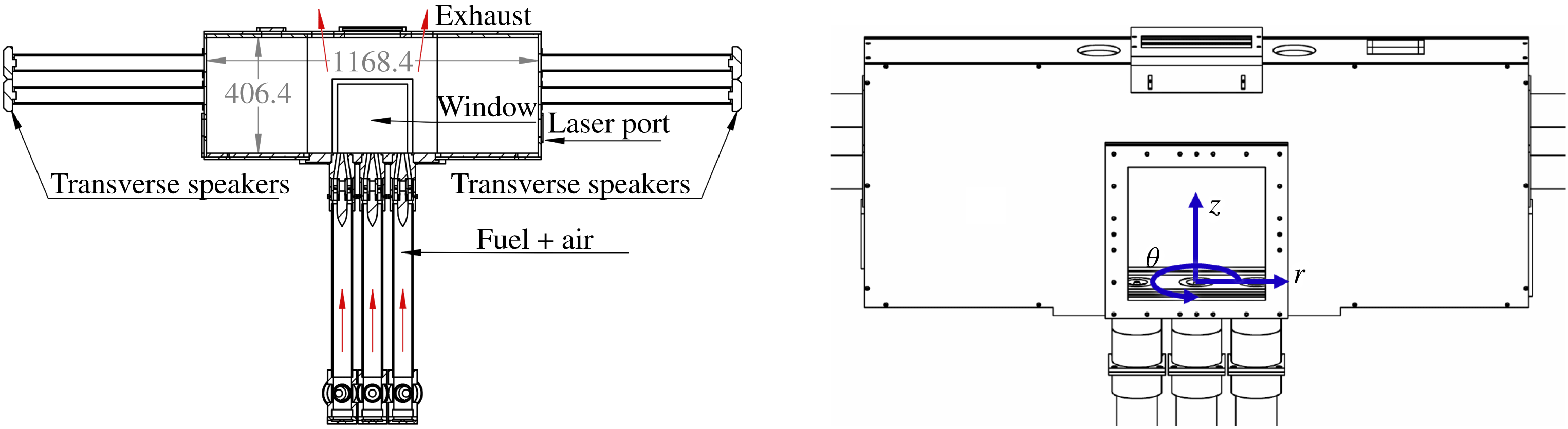
Figure 3 displays a cut section of the multi-nozzle combustor facility, a facility similar to Aguilar et al. (Reference Aguilar, Malanoski, Adhitya, Emerson, Acharya, Noble and Lieuwen2015). The combustor is designed to excite nominally one-dimensional transverse modes. Additionally, the nozzle conditions can be independently controlled, allowing for multiple flame configurations within the same combustor. Windows on the front and the back of the combustor make the centre nozzle and nozzle interaction regions visible. A third window located between the exhaust ports gives a top–down view of the centre nozzle. Additionally, there is a laser port on the side of the combustor allowing a laser sheet to bisect all three nozzles. Three nozzles were used to better simulate realistic boundary conditions on the centre nozzle.
Diagram of combustor with units in mm, flow path in red. Coordinate system shown on right in blue.

Figure 3 also shows transverse acoustic forcing tubes with speakers. The signal amplitude is held constant for each speaker, while the phase difference between the left and right speakers is either
 $0^{\circ }$
and in-phase (IP) or
 $180^{\circ }$
and out-of-phase (OP). These conditions create either a pressure anti-node or a velocity anti-node at the centre nozzle respectively, as verified previously (Malanoski et al.
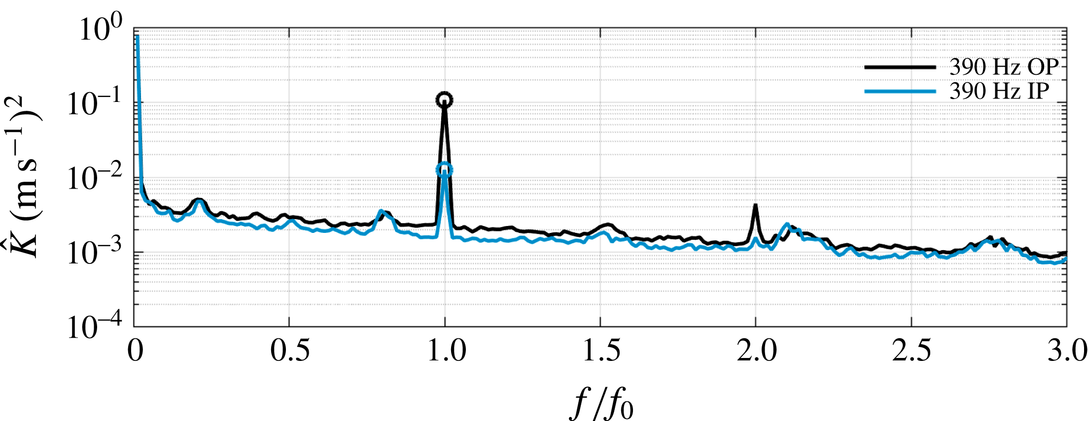
Reference Malanoski, Aguilar, Shin and Lieuwen2014). Four acoustic pressure transducers are located on the transverse acoustic tubes a distance 25.4 mm from the combustor, and six transducers are split evenly between the 3 mixing pipes and located 203 mm upstream of the dump plane 25.4 mm apart axially, for a total of ten acoustic transducers. Acoustic forcing is applied at 390 Hz in both the IP and OP configurations, where strong acoustic excitation is possible. The acoustic disturbance amplitude in the IP case in the axial direction is 2 % of the mean axial nozzle exit flow, while the OP case results in a transverse acoustic disturbance amplitude of 6 % of the mean axial nozzle exit flow. Figure 4 shows the spatially integrated power spectra from the measured PIV velocity field (sum of the magnitude of each velocity component squared) over the region
 $-0.75<r/D<0.75$
and
 $0.1<z/D<1.2$
, taken in the
 $r{-}z$
plane. The calculation approach of local spectra is further detailed in § 2.3. The spectra represent the spatial integration of the kinetic energy,
 $\hat{K}$
, of every point within the designated region. The figure shows that the response at the forcing frequency is clearly discernible and that the velocity anti-node (OP) case is an order of magnitude larger than the IP case, as predicted by an acoustic model of the combustor. Additionally, this figure shows that, outside of the peak at the forcing frequency and the first harmonic, there are no other prominent narrowband spectral features, suggesting that there are no globally unstable modes present.
Spectra of the fluctuating kinetic energy for the acoustically forced cases calculated from the stereo particle image velocimetry velocity fields.

Diagram of the nozzle with units in mm, flow path in blue.

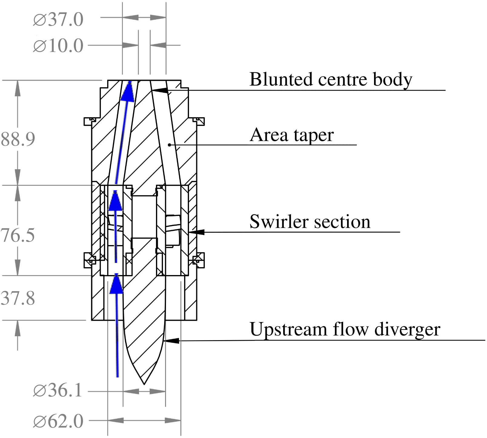
Figure 5 shows a cut section of the nozzle design. Premixed natural gas and air flow through a pipe to a flow diverger with an axisymmetric hyperbolic tangent profile to ensure a smooth entry into the annular passage with inner and outer radii of
 $r_{i,annulus}=18~\text{mm}$
and
 $r_{o,annulus}=31~\text{mm}$
, respectively. Next, the flow passes through an axial swirler with a geometric swirl of 0.6. The annular passage then converges over an axial distance of 88.9 mm, to
 $r_{o,nozzle}=18.5~\text{mm}$
and
 $r_{i,nozzle}=5~\text{mm}$
, so that the annular area is reduced by 50 %. The swirl number of the flow exiting the nozzle,
 $S_{n}$
, calculated from a stereoscopic particle image velocimetry (sPIV) measurement is approximately 0.5, calculated as the ratio of the tangential to axial momentum (Gupta, Lilley & Syred Reference Gupta, Lilley and Syred1984)
 $$\begin{eqnarray}S_{n}=\frac{\displaystyle \int _{0}^{D/2}\bar{u}_{\unicode[STIX]{x1D703}}\bar{u}_{Z}r^{2}\,\text{d}r}{{\displaystyle \frac{D}{2}}\displaystyle \int _{0}^{D/2}\bar{u}_{Z}^{2}r\,\text{d}r}.\end{eqnarray}$$
Three nozzles are placed linearly with a spacing of 2.9 nozzle diameters from centre to centre. Each nozzle has a nominal exit velocity of
 $25~\text{m}~\text{s}^{-1}$
, and a preheat temperature of 505 K at the nozzle. Room temperature natural gas enters the preheated air stream 10 pipe diameters upstream to ensure thorough fuel–air mixing. The centre nozzle is operated at an equivalence ratio of
 $\unicode[STIX]{x1D719}=0.95$
, and the outer nozzles at
 $\unicode[STIX]{x1D719}=0.6$
. The centre nozzle Reynolds number was approximately 23 000 based on the nozzle diameter and reactant viscosity. With this configuration, the centre flame was stabilized in the inner shear layer on the centre body (it does not also attach in the outer shear layer, but exists as a v-flame), and acts as a ‘pilot’ for the outer flames which ignite away from the nozzle.
2.2 Diagnostic techniques
This paper utilizes two measurement planes: a horizontal plane parallel to the dump plane centred about the middle nozzle and a vertical plane bisecting the three nozzles. These measurement planes are referred to as the
 $r$
–
 $\unicode[STIX]{x1D703}$
and
 $r{-}z$
planes respectively. The plane nomenclature is in reference to a cylindrical coordinate system centred on the middle nozzle with the axial direction in line with the axis of the nozzle, as shown by figure 3.
Simultaneous OH planar laser induced fluorescence (OH PLIF) and stereoscopic particle image velocimetry (sPIV) were taken at 5 kHz; related measurements have used similar diagnostics for velocity and flame position/heat release characterization (Steinberg et al.
Reference Steinberg, Boxx, Stöhr, Meier and Carter2012; Umeh, Rusak & Gutmark Reference Umeh, Rusak and Gutmark2012; Oberleithner et al.
Reference Oberleithner, Schimek and Paschereit2015). Here a double-pulsed laser with a wavelength of 527 nm, supplying 12 W per laser head, was used to place a laser sheet through the test section for sPIV. Two CMOS cameras with an interframe time of 400 ns were placed at equal angles to the plane containing the laser sheet and filtered to capture the scatter from the
 $0.5{-}1~\unicode[STIX]{x03BC}\text{m}\;\text{TiO}_{2}$
particles. For the
 $r$
–
 $z$
plane measurement, the PIV laser pulses were tested at 5, 10 and
 $14~\unicode[STIX]{x03BC}\text{s}$
apart, with
 $14~\unicode[STIX]{x03BC}\text{s}$
being chosen. This time spacing best balanced loss of particles due to out of plane motion and sufficient in-plane particle motion throughout the entire flow field, allowing the fastest particles to move approximately 6 pixels between laser pulses. However, this time spacing does introduce bias error due to loss of pairs near the nozzle exit where the azimuthal velocity is highest. Similarly the
 $r\unicode[STIX]{x1D703}$
measurement plane tested 3, 5 and
 $8~\unicode[STIX]{x03BC}\text{s}$
between laser pulses with
 $8~\unicode[STIX]{x03BC}\text{s}$
being chosen; this did not introduce significant bias error into the measurements. The OH PLIF technique was performed using a dye laser system tuned to 283.4502 nm pumped by an Nd:YAG laser at 532 nm. The OH fluorescence was captured using an additional high speed CMOS camera coupled to a gated high speed intensifier using a 45 mm UV CIRCA lens. Three cylindrical lenses (collimating:
 $f=50~\text{mm}$
diverging and
 $f=200~\text{mm}$
converging, thickness:
 $f=750~\text{mm}$
converging) were used on each of the lasers to create and condition the laser sheets before they were combined and passed into the combustor. The PIV and OH PLIF laser sheets were approximately 2 mm and 0.5 mm thick, respectively
The laser sheets for the
 $r{-}z$
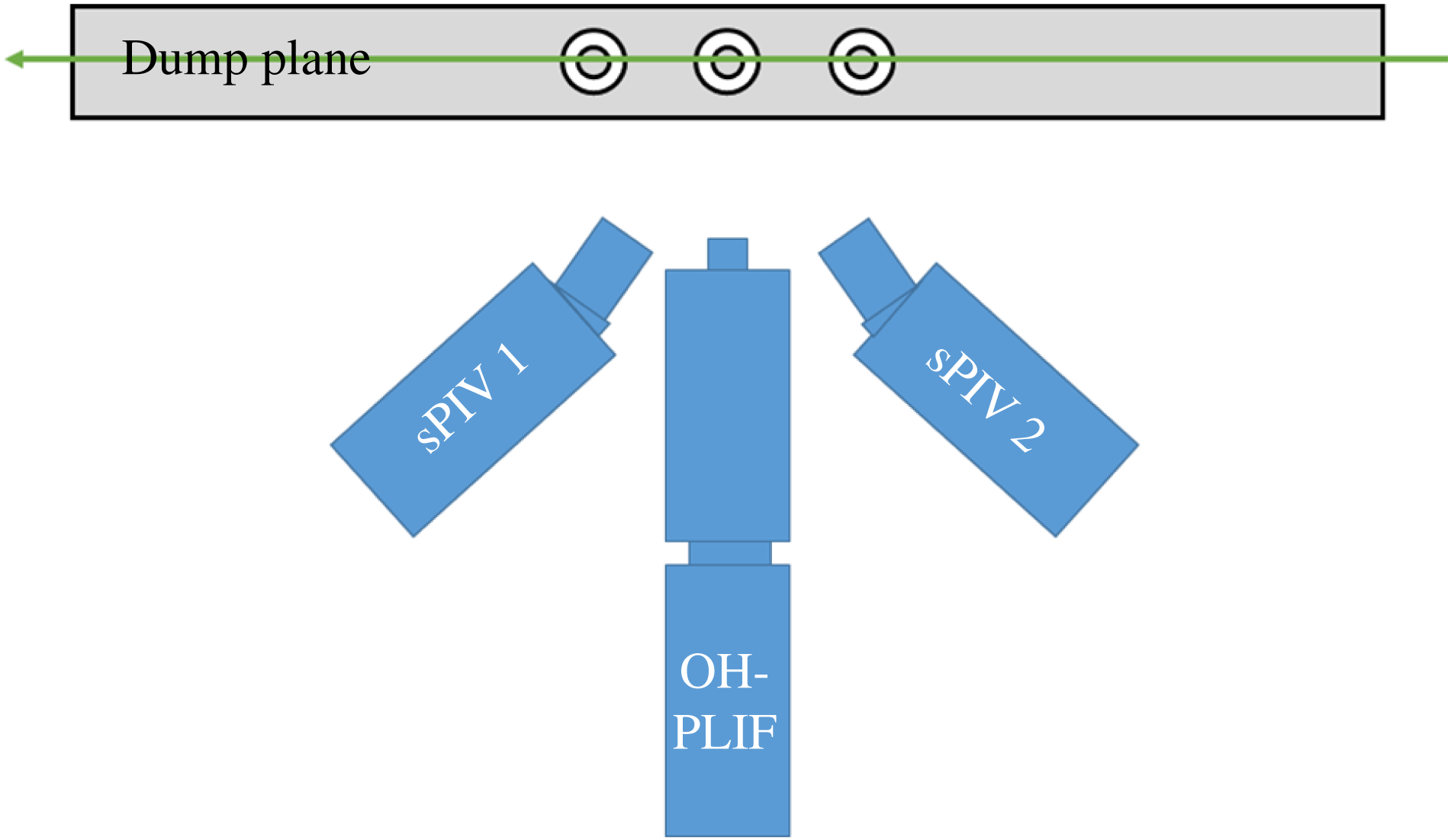
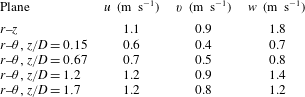
plane passed through the laser port on the side of the combustor and were imaged through the front window. The sPIV cameras were set at an angle of 35 degrees to the normal of the laser sheet and captured both forward and backscatter. The intensified PLIF camera was perpendicular to the laser sheet. Figure 6 shows a schematic of the camera set-up. Median uncertainties of the instantaneous velocities as calculated by DaVis are summarized in table 1. The higher amplitude uncertainties are located near the nozzle exit and at reflections. The uncertainty is tied to the particle seeding density and the spatial resolution of the camera. Because the
 $r$
–
 $z$
plane focused on a larger region than the
 $r$
–
 $\unicode[STIX]{x1D703}$
planes, it captured more area per pixel, and the uncertainty was higher.
Schematic of camera set-up in
 $r$
–
 $z$
plane with the vertical laser sheet in green.

Median random uncertainties of instantaneous velocities for each measurement plane and for the horizontal (
 $u$
), vertical (
 $v$
) and out-of-plane (
 $w$
) velocity components.

For the
 $r$
–
 $\unicode[STIX]{x1D703}$
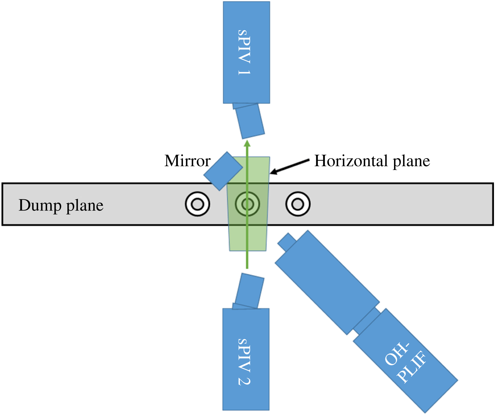
plane, the laser sheet passed through the front window of the combustor and out the back window. The two coplanar PIV cameras were set at
 $55^{\circ }$
from the normal of the laser sheet, looking down, and capturing both forward and back scatter from the particles in the flow. The laser pulses were set
 $8~\unicode[STIX]{x03BC}\text{s}$
apart. The intensified PLIF camera used a UV coated mirror to look down through the top window located between the exhaust ports. Measurements in the
 $r$
–
 $\unicode[STIX]{x1D703}$
planes were obtained at axial heights of
 $z/D=0.15$
, 0.67, 1.2 and 1.7. The jet merging occurs around
 $z/D=2$
, so most of these measurement domains are upstream of the flow field and shear layer merging. Figure 7 shows a schematic of the camera set-up for this plane. Table 1 shows the resulting flow field uncertainties for each plane as calculated by Davis.
Schematic of camera set-up in
 $r$
–
 $\unicode[STIX]{x1D703}$
planes with laser sheet in green.

Figure 8 shows the overlap of filtered PLIF and raw Mie scattering (sPIV) images for both the
 $r{-}z$
and
 $r{-}\unicode[STIX]{x1D703}$
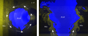
measurement planes. The more visible region of the Mie scattering image (yellow) contains more seeding particles and corresponds to the reactant jet exiting the annular nozzle. The region in blue shows where OH was present in the image and corresponds to where the combustion products can be found. The density jump across the flame is reflected in the change in number of seeding particles from the reactant jet to the blue product region, resulting in fewer visible particles in the product region. These images show that the flame is located in the inner shear layer of the seeded reactant jet. The nozzle exit can also be seen in the
 $r{-}\unicode[STIX]{x1D703}$
image – note that its centre is offset from the centre of the blue OH PLIF region because the sPIV viewing cameras are set at an angle and measuring a plane above the nozzle.
Mie scattering (yellow) and filtered OH PLIF image (blue) overlaid for
 $r$
–
 $\unicode[STIX]{x1D703}$
and
 $r$
–
 $z$
planes,
 $dt/2$
apart.

2.3 Post-processing techniques
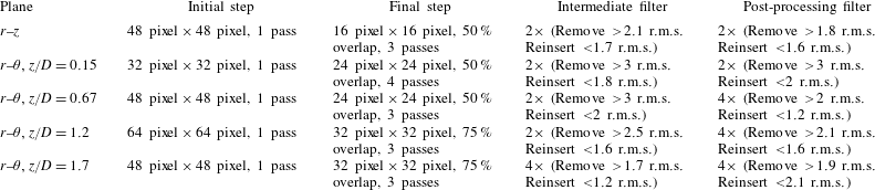
The two sets of image pairs acquired from the sPIV technique were processed using the Davis software from Lavision. This approach computes velocity vectors uses a digital cross-correlation algorithm (Willert & Gharib Reference Willert and Gharib1991) with a multi-pass approach (Soria Reference Soria1996) and two-dimensional (2-D) Gaussian subpixel interpolation (Willert & Gharib Reference Willert and Gharib1991). First, the background was subtracted using a sliding minimum, which also reduced reflections in the images but did not account for laser power variations. The calculation then used a particle normalization prior to applying a multi-pass, decreasing size correlation calculation. The initial passes contained no overlap and used a square window while the final pass used a Gaussian round window. After each correlation calculation, the vectors were filtered using the median filter that removes, then reinserts the vector values based on the root-mean-square (r.m.s.) of their neighbours. The uncertainty was calculated using the standard procedure built into Davis. The specific processing parameters for each measurement plane are shown in table 2. Additionally the Davis software was used to map all of the cameras with respect to the image plane.
sPIV processing settings for each plane.

The output vectors from Davis were in Cartesian coordinates, so the first post-processing step was to convert the vectors into the cylindrical coordinate system shown in figure 3. For the
 $r$
–
 $z$
plane, this was a trivial task. For the
 $r$
–
 $\unicode[STIX]{x1D703}$
plane, the velocity vectors were first interpolated from the Cartesian grid onto a polar grid using a cubic interpolation method so that the periodic azimuthal modes could be directly calculated. The polar grid was chosen such that the radial spacing of the grid was roughly equal to the spacing of grid points in the Cartesian grid. Its origin was selected as the point which maximized the symmetry of the time-averaged flow field. The instantaneous velocity components were then transformed into the cylindrical coordinate system.
A Fourier transform of the 7500 vector fields was performed at each point in the grid giving a frequency spectrum at each spatial location for each component of velocity. Each spectrum was estimated using Welch’s method with a window size of 0.2 s and a 75 % overlap, resulting in 27 ensembles and a spectral resolution of 5 Hz. The phase angles were calculated using a similarly averaged cross-power spectral density estimation with respect to a signal at the location of the maximum axial velocity standard deviation.
The PLIF images indicate the location of the flame edge. To very good approximation, the region where there is OH signal represents products, and the region of no signal represents reactants. To identify these regions, the instantaneous PLIF image is filtered and then binarized between zero (no signal) and one (signal). These instantaneous, binarized images are averaged to obtain a progress variable field,
 $\bar{c}$
, that represents the probability of flame products being present in a given region. The
 $\bar{c}=0.5$
iso-contour provides a convenient reference location to denote as the average position of the flame. Both phase-averaged and time-averaged progress variables were calculated. The phase-averaged
 $\bar{c}=0.5$
position was parameterized by the function,
 $R_{f}(\unicode[STIX]{x1D703},z,t^{\ast })$
, where
 $t^{\ast }$
represents the phase in the acoustic cycle. Similarly, the Fourier coefficient of the flame edge is given by
 $\hat{R}_{f}(\unicode[STIX]{x1D703},z,\unicode[STIX]{x1D714})$
.
3 Flow field decomposition and volumetric interpolation
3.1 Decomposition approach
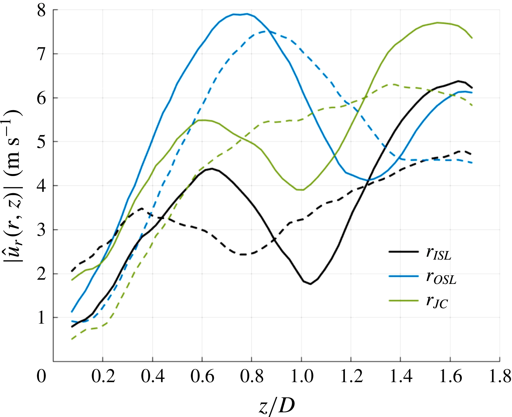
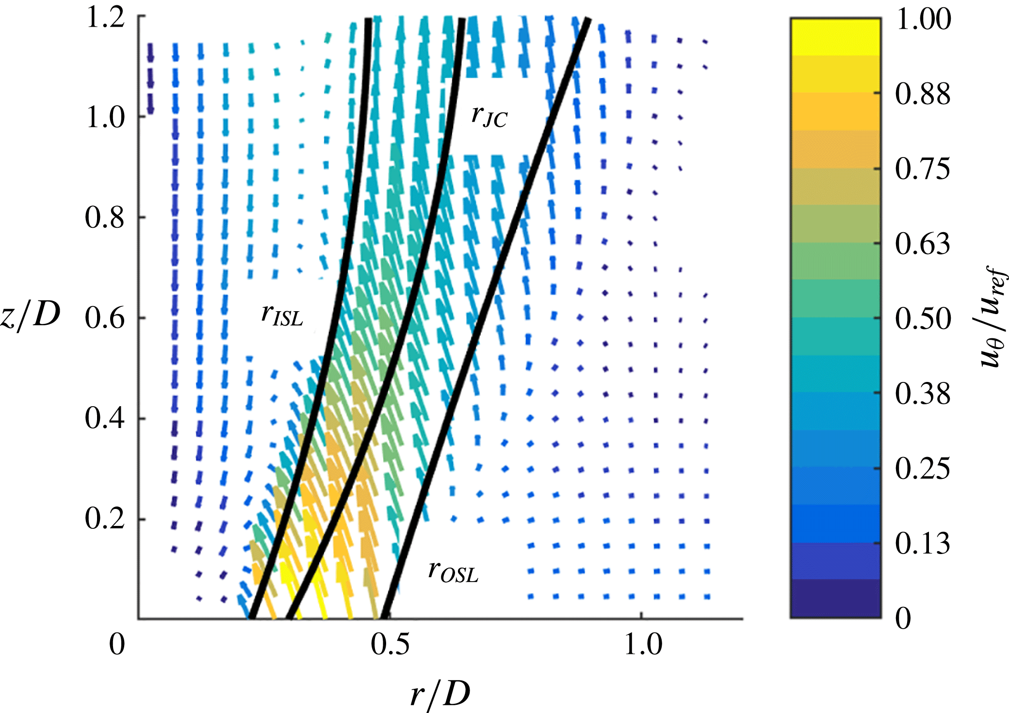
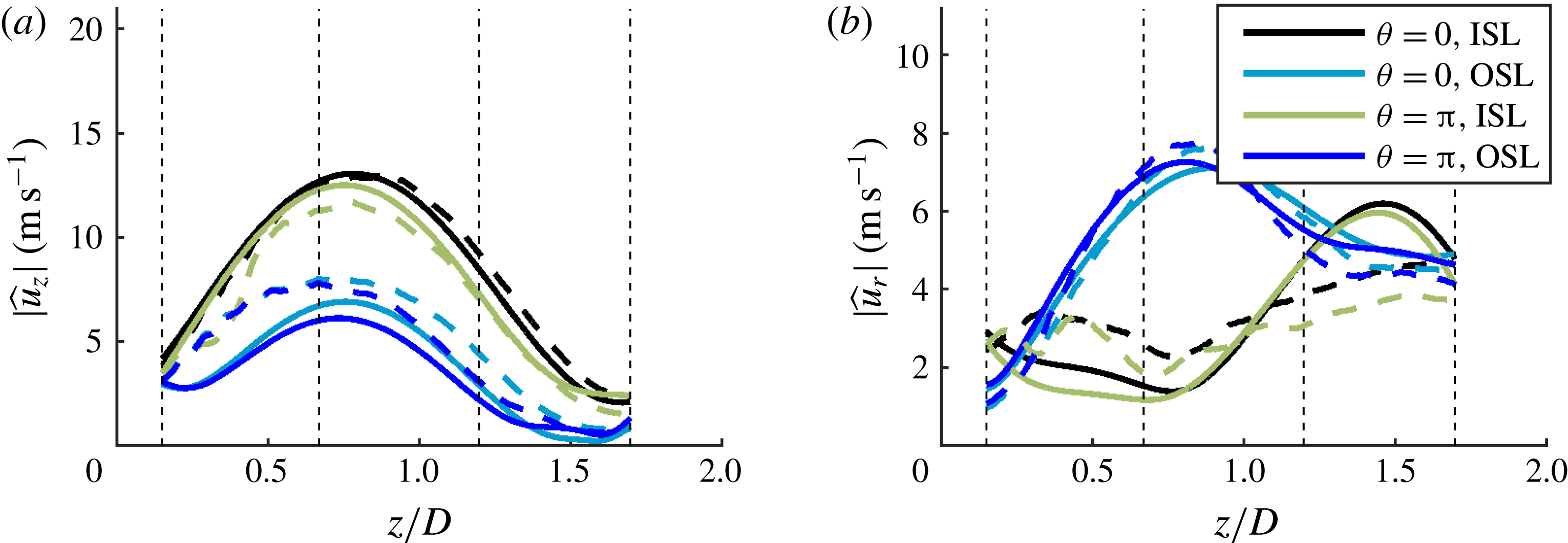
The measured velocity field can be decomposed into a time-averaged component, a coherent component at the forcing frequency and its harmonics, and the remaining, largely turbulent, component. The coherent component contains the superposition of acoustic and vortical (hydrodynamic) disturbances. Because the phase speeds of the acoustic and hydrodynamic disturbances are so different, their superposition manifests itself as clear interference patterns in the magnitude of the velocity, as shown in figure 9. The interference pattern manifests as the alternating peak–trough–peak pattern in the solid lines which represent the total measured disturbance. In order to focus on the hydrodynamic disturbances, the acoustic contribution was estimated and subtracted from the Fourier coefficients, using a similar method to O’Connor & Lieuwen (Reference O’Connor and Lieuwen2012a ). Given that the IP forcing case measured the centre nozzle at a velocity node, the transverse acoustic contribution to this case was negligible, and thus the technique was only applied to the transverse acoustics of the OP case. All OP data presented from this point forward will have the acoustic velocity component subtracted unless explicitly noted. As the transverse acoustic wave was nearly one-dimensional in nature, the transverse acoustic subtraction was only performed on the radial and azimuthal components of the flow field. The acoustic field was approximated by fitting a spatial sinusoidal function to the measured velocity field, at locations outside of the jet where the acoustic fluctuations dominated. Figure 9 shows the measured data and those with the acoustic subtraction performed on the OP case, showing the clear reduction of the interference pattern. The results are plotted along the shear layer lines and jet core defined in figure 10. The velocity envelopes in the shear layers still show some modulation, which will be discussed further in § 4.
Magnitude of transverse velocity fluctuations take from
 $r$
–
 $z$
data along inner shear layer (ISL), outer shear layer (OSL) and jet core (JC) without (solid) and with (dashed) acoustic subtraction for the 390 Hz OP case.

Sample time-average
 $r$
–
 $z$
plane showing shear layers and jet core locations.

Along each
 $r$
–
 $\unicode[STIX]{x1D703}$
plane, the Fourier coefficients, minus the estimated acoustic contribution, were decomposed into periodic azimuthal modes. Equation (3.1), seen below, shows the spatial decomposition of the frequency domain velocity measurements into periodic azimuthal modes:
 $$\begin{eqnarray}\hat{\boldsymbol{B}}_{m}(r,z,\unicode[STIX]{x1D714})=\frac{1}{2\unicode[STIX]{x03C0}}\int _{0}^{2\unicode[STIX]{x03C0}}\hat{\boldsymbol{u}}^{\prime }(r,\unicode[STIX]{x1D703},z,\unicode[STIX]{x1D714})\text{e}^{\text{i}m\unicode[STIX]{x1D703}}\,\text{d}\unicode[STIX]{x1D703}.\end{eqnarray}$$
Note again that the choice of sign convention of the periodic azimuthal modes was set such that
 $m<0$
is counter-swirling, and
 $m>0$
is co-swirling. Additionally the definition of the discrete Fourier coefficients of the velocity field used here results in units of
 $\text{m}~\text{s}^{-1}$
for both the Fourier coefficients and the helical mode coefficients. The Fourier coefficient of the
 $r$
–
 $\unicode[STIX]{x1D703}$
flame edge, calculated from the phase-averaged flame edge, can similarly be decomposed into azimuthal modes as
 $$\begin{eqnarray}\hat{R}_{f}(\unicode[STIX]{x1D703},z,\unicode[STIX]{x1D714})=\mathop{\sum }_{m=-\infty }^{\infty }\hat{R}_{m}(z,\unicode[STIX]{x1D714})\text{e}^{-\text{i}m\unicode[STIX]{x1D703}}/D,\end{eqnarray}$$
where
 $\hat{R}_{m}(z\unicode[STIX]{x1D714})$
represents the azimuthal mode coefficients at the given axial location and frequency, normalized by the nozzle exit diameter.
While the azimuthal coefficients of the flame edge only depend on the axial location, the azimuthal coefficients from the velocity data are functions of both
 $r$
and
 $z$
. Thus, various approaches were used to reduce the dimensionality of the velocity data sets to facilitate data presentation. First, the helical mode magnitudes are averaged radially as follows:
 $$\begin{eqnarray}\bar{\boldsymbol{B}}_{m}(\unicode[STIX]{x1D714},z)=\int _{0}^{R}|\hat{\boldsymbol{B}}_{m}(\unicode[STIX]{x1D714},z,r)|r\,\text{d}r/R^{2},\end{eqnarray}$$
where the outer limit of the integration
 $R$
is the outer edge of the time-averaged outer shear layer in the
 $r$
–
 $z$
plane, defined as
 $$\begin{eqnarray}\frac{\unicode[STIX]{x2202}(\bar{u}_{Z}(R,z))}{\unicode[STIX]{x2202}r}\equiv 0.5\ast \min \left(\frac{\unicode[STIX]{x2202}(\bar{u}_{Z}(r,z))}{\unicode[STIX]{x2202}r}\right).\end{eqnarray}$$
 $\bar{\boldsymbol{B}}_{m}$
is the area weighted integral of the coefficient magnitudes from the centreline to the edge of the outer shear layer. This approach works well for identifying which modes are dominant at each axial location but hides the spatial distribution of these modes. As an additional approach to also reduce the dimensionality of the velocity data, while presenting some information about both their radial and axial distributions, reference lines in the
 $r$
–
 $z$
plane are defined. First, reference inner shear layer (ISL) and outer shear layer (OSL) lines were defined based on time-averaged velocity. The ISL and OSL are calculated as the location of minimum and maximum mean azimuthal vorticity, respectively, as a function of axial distance. An additional reference line, the jet core (JC) is calculated as the line of maximum velocity magnitude in the
 $r$
–
 $z$
plane. Figure 10 shows the locations of these three lines on a sample time-averaged
 $r$
–
 $z$
flow field where the colour represents the azimuthal velocity normalized by a reference bulk axial velocity out of the nozzle,
 $u_{ref}=28.8~\text{m}~\text{s}^{-1}$
.
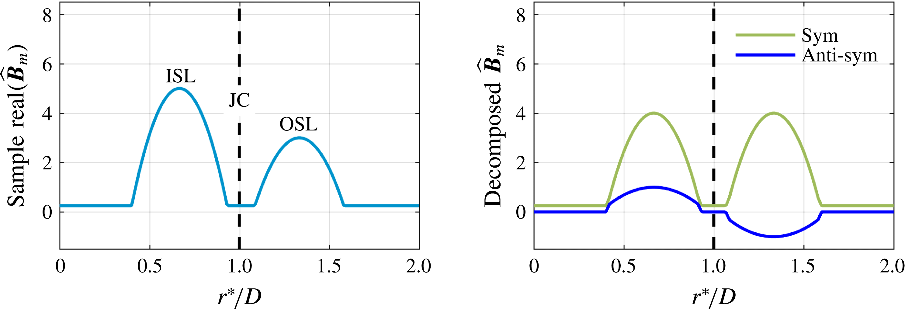
As will be shown in the next section, the axial hydrodynamic modes consist of velocity fluctuations dominantly located in the shear layers, with different relative amplitudes and phases in the ISL and OSL, as shown notionally in figure 11(a). This suggests decomposing the ISL and OSL disturbances into those that are symmetrically and anti-symmetrically oscillating with respect to each other about the JC, as illustrated by figure 11(b). This was done using an even–odd decomposition in a coordinate system that is centred at the jet core, defined by
 $(r_{2}^{\ast }(z)z)$
, using
 $$\begin{eqnarray}\left.\begin{array}{@{}c@{}}\hat{\boldsymbol{B}}_{m,s}(r_{2}^{\ast },z)=0.5(\hat{\boldsymbol{B}}_{m}(r_{2}^{\ast },z)+\hat{\boldsymbol{B}}_{m}(-r_{2}^{\ast },z)),\\ \hat{\boldsymbol{B}}_{m,a}(r_{2}^{\ast },z)=0.5(\hat{\boldsymbol{B}}_{m}(r_{2}^{\ast },z)-\hat{\boldsymbol{B}}_{m}(-r_{2}^{\ast },z)),\\ r_{2}^{\ast }(z)=r-r_{JC}(z),\end{array}\right\}\end{eqnarray}$$
where
 $r_{ISL}$
is the location of the ISL,
 $r_{JC}$
is the location of the JC,
 $\hat{\boldsymbol{B}}_{m,s}$
is the symmetric component of the helical mode and
 $\hat{\boldsymbol{B}}_{m,a}$
is the anti-symmetric component of the helical mode. Note that symmetric and anti-symmetric are reversed for the radial velocity helical modes. This decomposition is similarly motivated by hydrodynamic stability analysis of related velocity fields (i.e. annular, swirling flows with inner and outer shear layers) – e.g. Manoharanet al. (Reference Manoharan, Emerson, Smith, Douglas, Lieuwen and Hemchandra2017) refers to the anti-symmetric and symmetric shear layer modes as ‘sinuous’ and ‘varicose’ modes respectively.
Example (not data) azimuthal mode distribution illustrating symmetric and anti-symmetric decomposition of the real part of velocity disturbances about the JC, following (3.5).

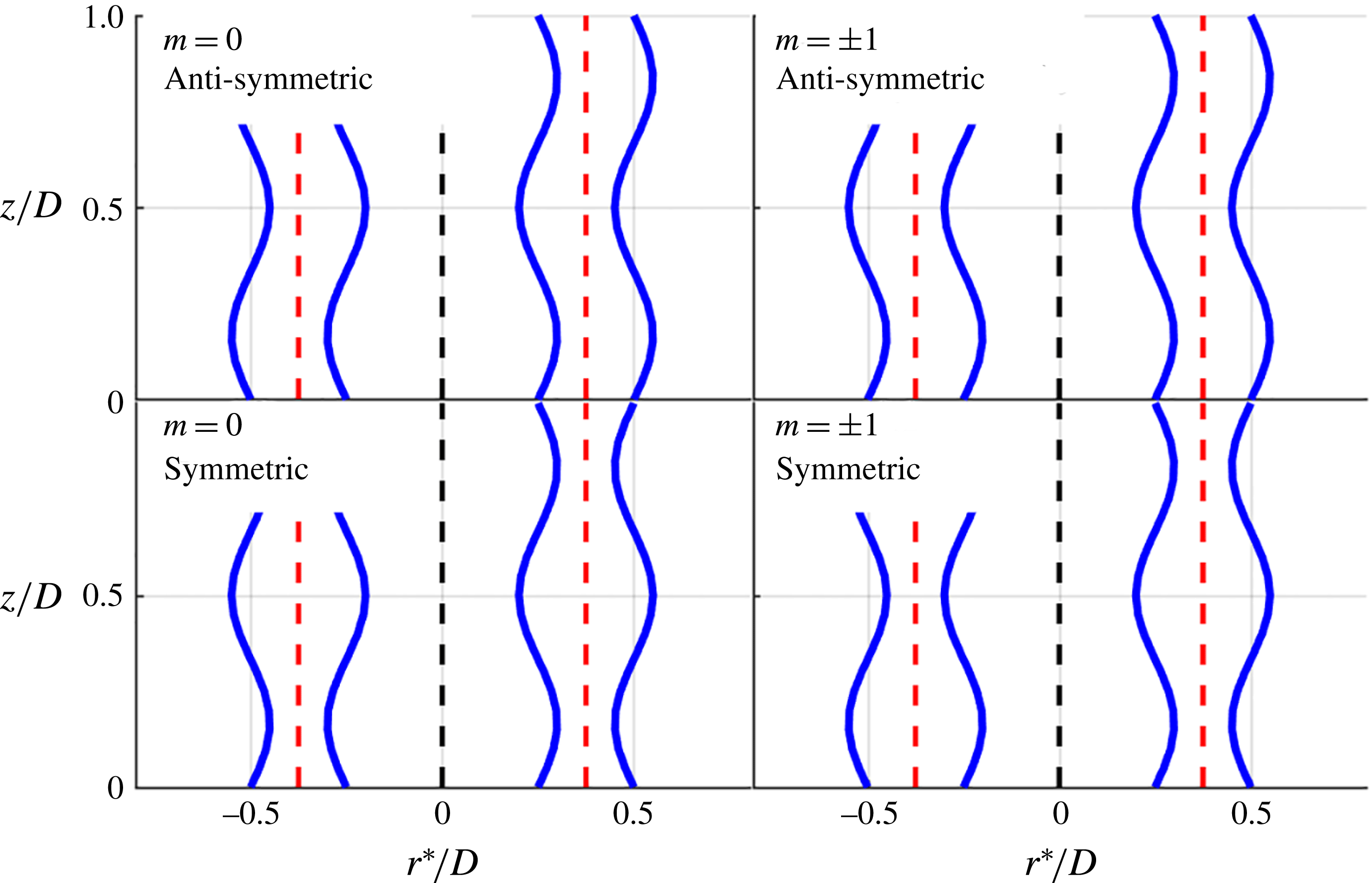
The physical manifestation of these symmetric and anti-symmetric disturbance modes for the
 $m=0$
and 1 modes are illustrated in figure 12. The anti-symmetric decomposition represents a flapping jet motion in two dimensions. Essentially the radial disturbance causes the jet to move across the time-average JC. This causes the axial velocity to increase in one shear layer and decrease in the other, the anti-symmetric mode of the axial velocity. On the other hand the symmetric decomposition captures the modulation of the jet width. The radial disturbances compress or stretch the 2-D jet, resulting in the symmetric axial velocity oscillations in the shear layers.
The helical mode number determines the periodicity of the decomposed modes about the centreline. If the mode is axisymmetric,
 $m=0$
, then the anti-symmetric component represents the periodic expansion of the jet. Similarly the
 $m=0$
symmetric component represents the periodic modulation of the jet annular width. For the
 $m=\pm 1$
modes, the anti-symmetric component represents the precession of the jet about the centreline while the symmetric component can represent local mass flow oscillations with no net total mass flow oscillation due to azimuthal cancellation.
Illustration of flow field manifestation of symmetric and anti-symmetric modes as translation and expansion of annular jet due to radial disturbances in the ISL and OSL with the JC in red (dashed) and the centreline in black (dashed).

3.2 Interpolation approach
As noted above, measurements with the same forcing frequency were obtained along five planes – one
 $r$
–
 $z$
plane and four
 $r$
–
 $\unicode[STIX]{x1D703}$
planes. The
 $r$
–
 $\unicode[STIX]{x1D703}$
measurements are particularly useful, as they allow us to determine the amplitude and phase of all helical modes,
 $\hat{\boldsymbol{B}}_{m}(r,z,\unicode[STIX]{x1D714})$
at that
 $z$
location, as well as to decompose each helical mode into symmetric and anti-symmetric disturbances. However, since these measurements are only obtained at four different
 $z$
locations, there are also a number of questions about how these modes evolve between measurement planes. In contrast, the
 $r$
–
 $z$
plane measurement has information on the velocity field/flame position at every
 $z$
location, but it is not possible to determine the relative amplitude of the different helical modes that are being superposed to give the resultant measurement. This section describes an interpolation approach to resolve the
 $z$
distribution of the
 $\hat{\boldsymbol{B}}_{m}(r,z,\unicode[STIX]{x1D714})$
coefficients.
The basic approach is to use a set of radial, azimuthal and axial basis functions to fit the data (defined with respect to the coordinate system described below), and use a least squares minimization approach to fit the data sets. The simplest option for these basis functions is a linear combination of functions defined with respect to the
 $(r,\unicode[STIX]{x1D703},z)$
coordinate system. The problem with that approach is that the flow streamlines are curved in the
 $r$
–
 $z$
coordinates (see figure 10), meaning that the velocity profiles in the
 $z$
direction vary strongly as a function of
 $r$
. This makes the coordinate dependence of the basis functions inseparable. In order to more nearly separate the basis functions into a radial and axial component, we use a curvilinear coordinate system
 $(r^{\ast },z/D)$
created by normalizing the radial direction with the radius of the jet core line at each axial location,
 $r^{\ast }=r/r_{JC}$
. The basis functions for the interpolation can then be written as
 $$\begin{eqnarray}F(r^{\ast },\unicode[STIX]{x1D703},z)=\mathop{\sum }_{i}\mathop{\sum }_{j}\mathop{\sum }_{k}a_{ijk}f_{i}(r^{\ast })g_{j}(z)h_{k}(\unicode[STIX]{x1D703}),\end{eqnarray}$$
where
 $f_{i}(r^{\ast })$
represents a radial basis function,
 $g_{j}(z)$
represents an axial basis function,
 $h_{k}(\unicode[STIX]{x1D703})$
represents an azimuthal basis function and
 $a_{ijk}$
represents the fit coefficients for the combined terms. The following basis functions were chosen based upon extensive analysis of the measurements, with the objective of utilizing functions that naturally fit the measurements with a minimal number of coefficients:
 $$\begin{eqnarray}\left.\begin{array}{@{}c@{}}\displaystyle \mathop{\sum }_{l=1}^{N_{r}+1}f_{l}(r^{\ast })=1+\displaystyle \mathop{\sum }_{m=1}^{N_{r}}\sin \left(m\unicode[STIX]{x03C0}\left({\displaystyle \frac{r^{\ast }}{r_{max}^{\ast }}}\right)\right),\\ \displaystyle \mathop{\sum }_{l=1}^{N_{z}+2}g_{l}(z)=1+\displaystyle \mathop{\sum }_{m=1}^{N_{z}+1}z^{m-1}\exp (\text{i}\unicode[STIX]{x1D719}(z))\\ \displaystyle \mathop{\sum }_{l=1}^{2N_{\unicode[STIX]{x1D703}}+1}h_{l}(\unicode[STIX]{x1D703})=\displaystyle \mathop{\sum }_{m=-N_{\unicode[STIX]{x1D703}}}^{N_{\unicode[STIX]{x1D703}}}\exp (-\text{i}m\unicode[STIX]{x1D703}).\end{array}\right\}\end{eqnarray}$$
The function
 $\unicode[STIX]{x1D719}(z)$
is a second-order polynomial fit to the phase lines in the shear layers as calculated from the
 $r$
–
 $z$
plane data, which allows the axial wavenumber of the dominant disturbances to be well approximated. The benefit of this phase speed fit is that the polynomial multiplying this term only has to capture the magnitude of the axial disturbance. Thus the mode shapes and phase speeds of the dominant disturbances are well captured. Finally, it should be noted that summing the axial and radial terms at a given axial–radial location gives the coefficients of the helical modes times the azimuthal periodicity term; i.e.
 $$\begin{eqnarray}\hat{\boldsymbol{B}}_{m}(r^{\ast },z)\text{exp}(-\text{i}m\unicode[STIX]{x1D703})=\mathop{\sum }_{j}\mathop{\sum }_{k}a_{jkl}f_{j}(r^{\ast })g_{k}(z).\end{eqnarray}$$
The radial fit to the data was given by choosing
 $N_{r}=15$
.
 $N_{\unicode[STIX]{x1D703}}$
was chosen as 3 giving a total of 7 helical modes (note that the
 $|m|>3$
modes contain a negligible amount of the energy at the forcing frequency as shown later). Four different axial locations were measured allowing for 4 different axial terms to be used without introducing oscillations between axial locations.
 $N_{z}$
was chosen as 2 so that the axial envelope of the helical modes could be approximated by a second-order polynomial. Data outside of
 $z/D\in [0.05,1.7]$
and
 $r^{\ast }\in [0,2]$
were ignored for the least squares fit.
The PIV Fourier coefficients from the
 $r$
–
 $\unicode[STIX]{x1D703}$
and
 $r$
–
 $z$
planes were then given a common phase reference by using the common radial and axial velocity measurement. Each point used in the least squares fit was weighted by its representative measurement area. The fit was applied separately to each of the three velocity components, with a resultant weighted
 $R^{2}$
value of more than 0.9 for its overall fit to the data. Figure 13 shows the resulting fitted axial velocity and radial velocity magnitudes along the ISL and OSL compared to the original data for the OP case taken from the
 $r$
–
 $z$
plane. The overall trends of the magnitudes and the relative amplitudes of the magnitudes are well captured in all components and forcing cases; for example, the magnitude of the first peak typically differs by no more than 5 %. The differences are due to the fact that the fit is a weighted regression between the separate
 $r$
–
 $z$
and
 $r$
–
 $\unicode[STIX]{x1D703}$
measured values.
Comparison of fit velocity magnitudes with
 $r$
–
 $z$
measured data along ISL and OSL for the 390 Hz OP forcing case. Solid lines are interpolated data while dashed lines are measured from
 $r$
–
 $z$
plane.

4 Results and analysis
4.1 Basic flow structure and response
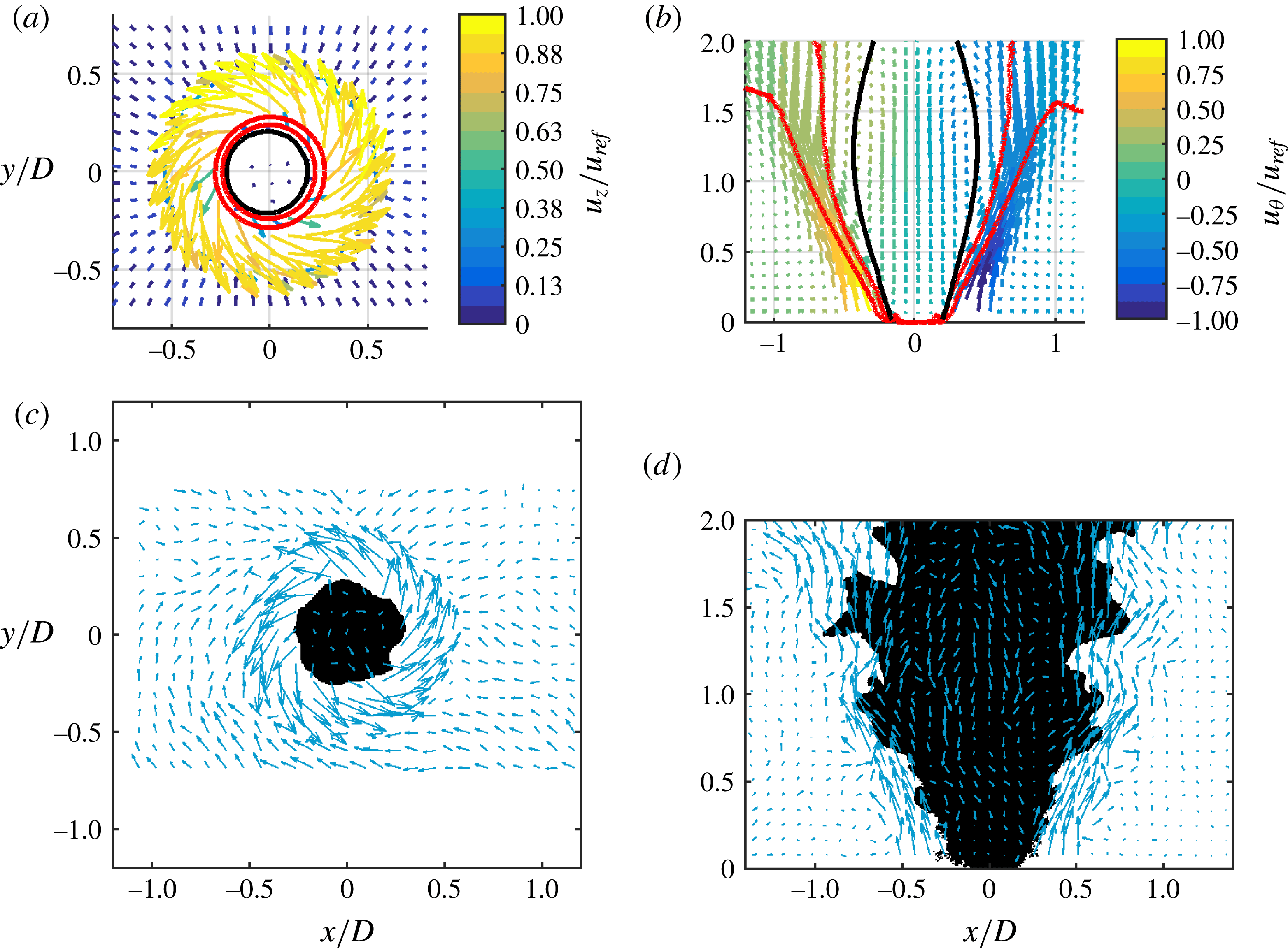
Figure 14 plots a typical time-averaged (a,b) and instantaneous (c,d) image of the flow field for the
 $r$
–
 $\unicode[STIX]{x1D703}$
(a,c) and the
 $r{-}z$
(b,d) measurement planes. Overlaid on the time-averaged figure are the red
 $\bar{c}=0.2$
and
 $\bar{c}=0.8$
flame progress variable contours in red and the axial velocity stagnation contour in black. The colour of the arrows in the time-averaged images quantifies the out-of-plane velocity component. Overall, the flow consists of an annular jet of fluid, surrounding a central recirculation zone that closes
 $z=2.5$
nozzle diameters downstream. The flame progress variable field lines show that the flame stabilizes in the ISL and show that the flame brush grows with downstream distance, eventually crossing into the OSL. The instantaneous images clearly demonstrate the presence of both fine scale and coherent, large scale disturbances on the flame.
Sample time-averaged flow field with flame brush boundaries in red
 $(0.2\leqslant \bar{c}\leqslant 0.8)$
and axial stagnation overlay in black (a,b) and sample instantaneous unforced flow field overlaid on binarized and inverted PLIF image (c,d) for
 $r{-}\unicode[STIX]{x1D703}$
at
 $z/D=0.15$
(a,c) and
 $r{-}z$
(b,d).

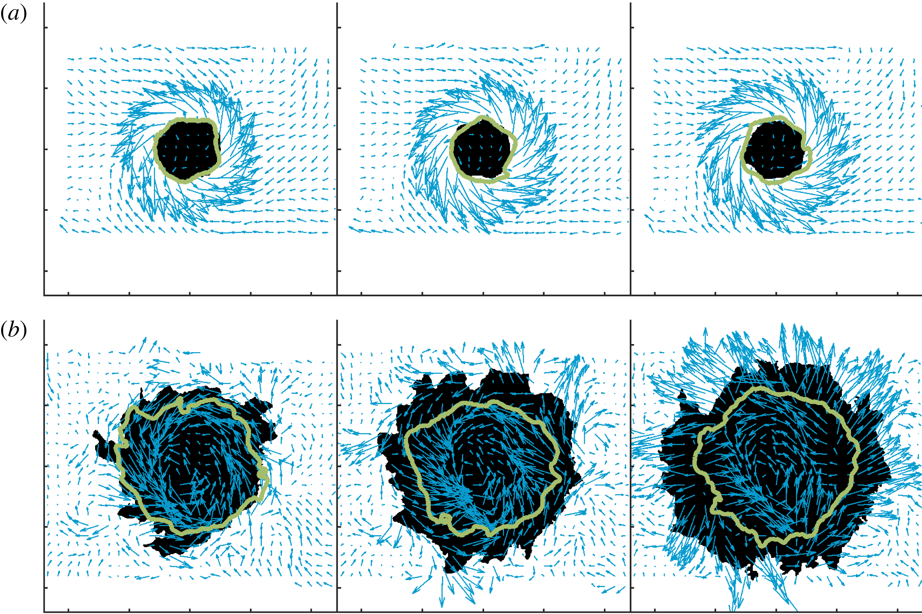
We next consider the effect of the different forcing configurations separately. Consider the IP forcing case first – this forcing configuration results in a symmetric pressure field across the nozzle, a pressure anti-node, and strong axial forcing of the nozzle acoustics (sometimes referred to as injector coupling), as described by Blimbaum et al. (Reference Blimbaum, Zanchetta, Akin, Acharya, O’Connor, Noble and Lieuwen2012). Figure 15 plots a series of instantaneous vector fields and OH PLIF images at different axial locations. The black region denotes the current OH PLIF signal while the green line denotes the outline of the OH PLIF region at a time instant roughly half a cycle earlier (more precisely,
 $168^{\circ }$
). The near coincidence of these two lines at the
 $z/D=0.15$
location shows the relatively weak flame motion, due to flame attachment near the nozzle outlet. At the
 $z/D=1.2$
location, however, the flame is clearly flapping in a nearly axisymmetric motion, as indicated by the significant differences in location between the two lines. In addition, there is clearly a significant degree of increased fine scale wrinkling.
Sequential IP forcing images in
 $r$
–
 $\unicode[STIX]{x1D703}$
for (a)
 $z/D=0.15$
and (b)
 $z/D=1.2$
showing velocity vectors and binarized OH PLIF. The black region denotes the instantaneous OH PLIF signal while the green line denotes its outline at a time instant
 $168^{\circ }$
earlier.

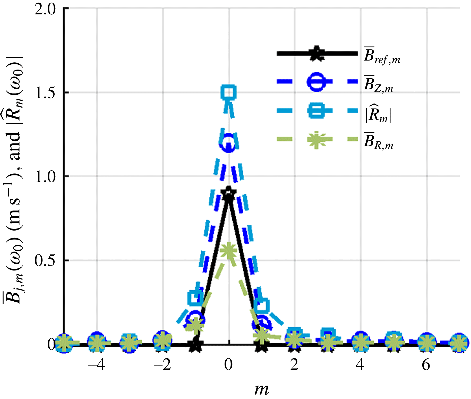
Figure 16 shows the azimuthal mode decomposition of two velocity components,
 $u_{r}$
and
 $u_{z}$
, and the flame position,
 $R_{f}$
, at a height of
 $z/D=0.15$
for the IP forcing case from the non-interpolated data. Additionally shown are radially integrated reference coefficients,
 $\bar{B}_{ref,m}$
, calculated from
 $$\begin{eqnarray}\bar{B}_{ref,m}=\int _{0}^{R}|\hat{B}_{ref,m}|r\,\text{d}r,\end{eqnarray}$$
where
 $\hat{B}_{ref,m}$
is calculated from a Jacobi–Anger decomposition taken from O’Connor et al. (Reference O’Connor, Acharya and Lieuwen2015). Specifically, expanding a one-dimensional, transverse acoustic wave into helical mode coefficients in an (
 $r,\unicode[STIX]{x1D703}$
) coordinate system using a Jacobi–Anger expansion gives,
 $$\begin{eqnarray}F(r,\unicode[STIX]{x1D703},k)=\mathop{\sum }_{m=-\infty }^{\infty }\hat{B}_{ref,m}(kr)\text{e}^{\text{i}m\unicode[STIX]{x1D703}}.\end{eqnarray}$$
In the case where
 $r=0$
corresponds to a pressure node/velocity anti-node, then the acoustic velocity field can be approximate as
 $F(x)=\cos kx$
, where
 $x$
denotes the direction of the transverse wave and
 $k=\unicode[STIX]{x1D714}/c$
denotes the acoustic wave number. This one-dimensional functions can be written as a superposition of two-dimensional disturbances in a nozzle-centred polar coordinate system, as:
 $$\begin{eqnarray}\hat{B}_{ref,m}=i^{m-1}J_{m}(kr).\end{eqnarray}$$
Note that this implies dominant
 $m=\pm 1$
modes, as well as an infinite number of successively decreasing amplitude odd modes; even modes are not excited. In contrast, even modes are excited as
 $$\begin{eqnarray}\hat{B}_{ref,m}=i^{m}J_{m}(kr),\end{eqnarray}$$
for the case where
 $r=0$
corresponds to a pressure anti-node/velocity node,
 $F(x)=\text{sin}(kx)$
, with the
 $m=0$
mode being dominant; odd modes are not excited.
The
 $\hat{B}_{ref,m}$
coefficients provide an estimate of the forcing provided by the acoustics to the hydrodynamic field. The data clearly show the strong excitation of the
 $m=0$
mode, suggested by the discussion of figure 15, consistent with prior measurements and predictions. The data also show the presence of the weaker
 $m=\pm 2$
modes. While much weaker than the
 $m=0$
mode, they are also much larger than suggested by the reference line, which is an indicator of the relative excitation that the acoustic disturbance provides to each mode. This may be a reflection of the fact that these modes have had some spatial distance to develop (i.e. the data are taken
 $0.15D$
downstream from the nozzle outlet) or that there are ‘imperfections’ of the acoustic excitation field relative to the model one-dimensional field,
 $\sin kx$
, used for the reference coefficient calculation. The other azimuthal modes are non-zero, presumably a manifestation of the turbulent fluctuations in the flow. Nonetheless, it is the strong
 $m=0$
oscillations which lead to axisymmetric disturbances convecting downstream in the shear layers, similarly causing strong axisymmetric wrinkling of the flame.
Radially integrated helical mode coefficients of velocity fluctuations (
 $\bar{\boldsymbol{B}}_{m}$
) for the 390 Hz IP forcing case (
 $z/D=0.15$
) and a scaled flame edge helical mode coefficient magnitude (
 $\hat{R}_{m}$
) compared to the scaled reference velocity function from the introduction integrated over the domain.

The resulting heat release excited by these hydrodynamic flow disturbances depends strongly upon which helical mode is present. Phase cancellation from different azimuthal locations causes helical modes to excite minimal heat release oscillations when they are integrated azimuthally, even though they may excite strong flame flapping. Rather, the spatially integrated heat release is most affected by axisymmetric,
 $m=0$
disturbances (Acharya, Shin & Lieuwen Reference Acharya, Shin and Lieuwen2013). This can be seen by considering the integral
 $\int \text{e}^{\text{i}m\unicode[STIX]{x1D703}}\,\text{d}\unicode[STIX]{x1D703}$
and noting that it is only non-zero for
 $m=0$
. In other words, the dominant hydrodynamic mode exciting heat release oscillations and local flame wrinkling is different (Worth & Dawson Reference Worth and Dawson2013a
,Reference Worth and Dawson
b
).
Consider next the OP forcing case. In this case, a pressure node and a velocity anti-node are nominally located at the centreline; i.e. the velocity is
 $180^{\circ }$
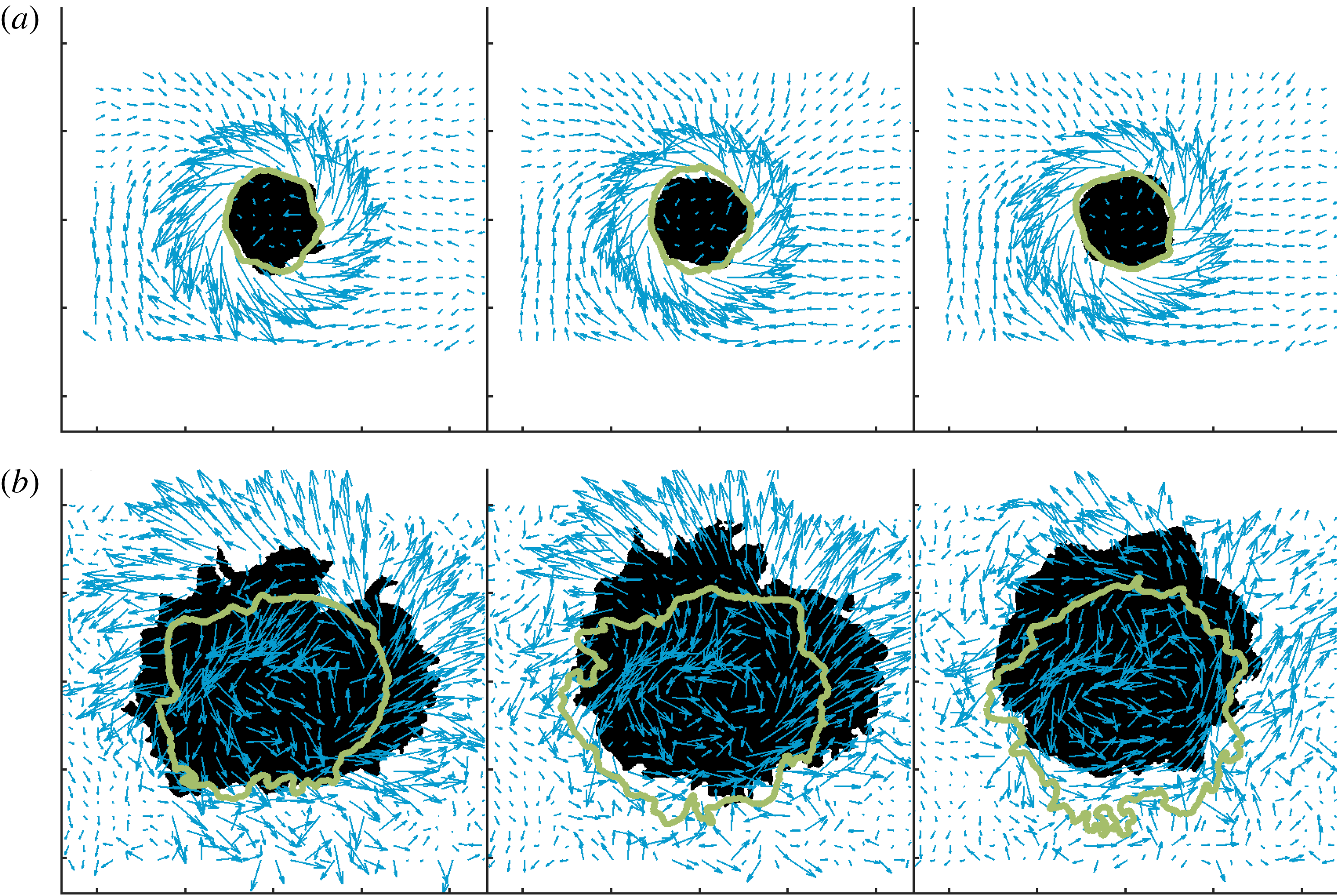
out of phase across the centreline. This results in a strong side-to-side flapping of the flame and flow field. Figure 17 shows sequential overlaid OH PLIF and vector field images for the OP forcing case with the green line representing the outline of the OH signal at a time instant approximately half a cycle earlier (
 $168^{\circ }$
). Again, near the nozzle exit the two lines are nearly coincident and circular, due to the flame nearly conforming to the shape of the circular centre body where it is attached. Farther downstream, the strong side-to-side flapping of the flame and flow field is clearly evident.
Sequential OP forcing images in
 $r$
–
 $\unicode[STIX]{x1D703}$
for (a)
 $z/D=0.15$
and (b)
 $z/D=1.2$
showing velocity vectors and OH PLIF. The black region denotes the current OH PLIF signal while the green lines denotes its outline at a time instant
 $168^{\circ }$
earlier.

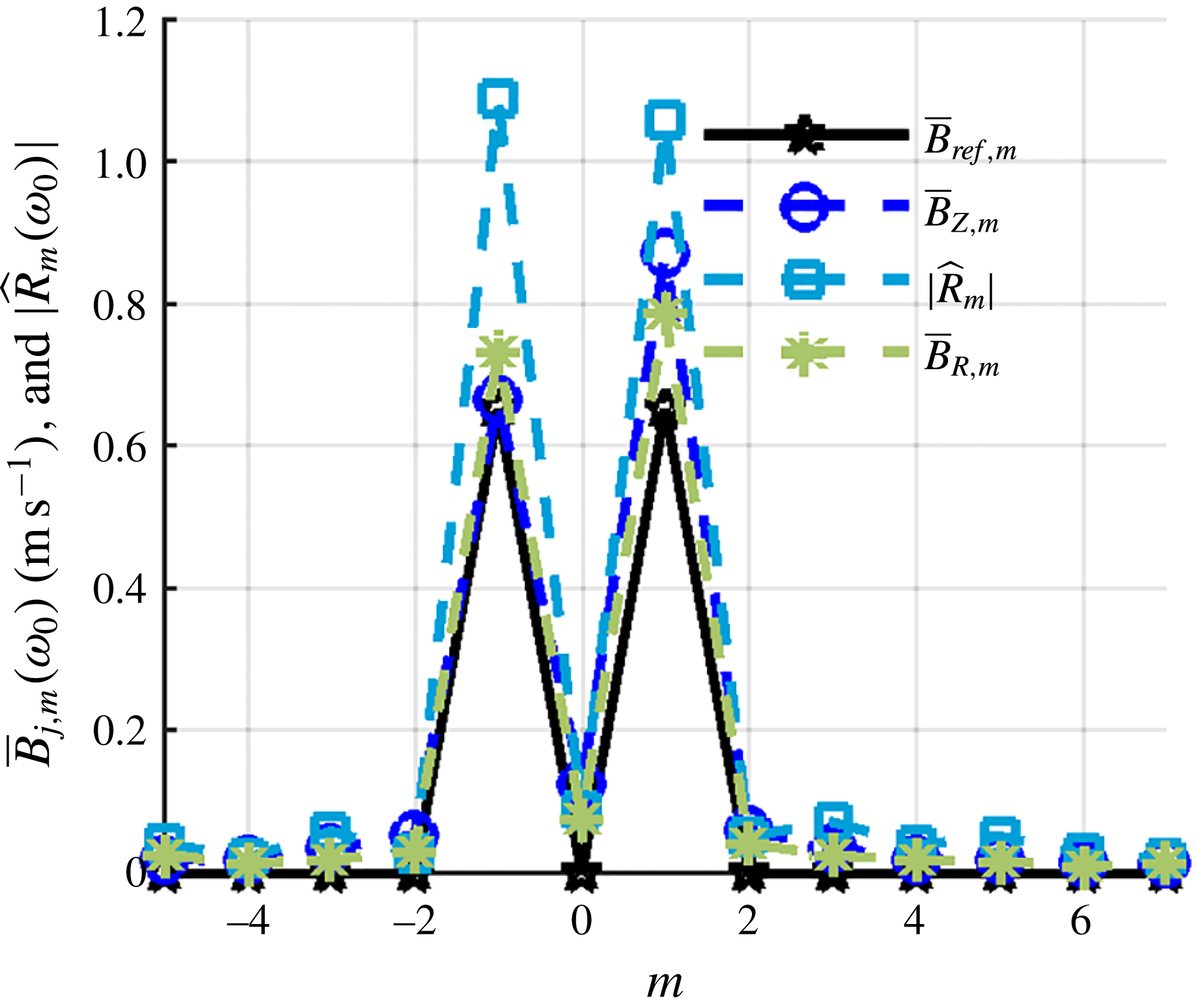
The strong side-to-side flapping motion is a manifestation of dominant
 $m=\pm 1$
modes, as quantified in figure 18 and consistent with the discussion in the introduction. Also overlaid for reference are radially integrated coefficients,
 $\bar{B}_{ref,m}$
, from the Jacobi–Anger expansion shown in the earlier footnote. These helical disturbances manifest themselves as staggered vortices and asymmetric flapping of the flame sheet. Note how the amplitude of the higher-order helical disturbances, such as
 $m=\pm 3$
, are slightly larger than predicted by the model velocity field. Again, this is likely a manifestation of the fact that the data are taken at
 $z/D=0.15$
, where they have had some time to spatially develop. Additionally this could be due to the random fluctuations associated with turbulence being captured by the decomposition. In addition, note the small but non-zero
 $m=0$
mode, due to some inherent axial motions induced at the nozzle exit.
Radially integrated helical mode coefficients of velocity fluctuations
 $(\bar{\boldsymbol{B}}_{m})$
for the 390 Hz OP forcing case
 $(z/D=0.15)$
and a scaled flame edge helical mode coefficient magnitude
 $(\hat{R}_{m})$
compared to the scaled reference velocity function from the introduction integrated over the domain.

While also alluded to in the introduction, it is worth contrasting these results with the natural global instabilities of swirling jets. In those cases, the flow field is dominated by a single global mode (Billant et al.
Reference Billant, Chomaz and Huerre1998; Liang & Maxworthy Reference Liang and Maxworthy2005). In contrast, forcing enables the selective excitation of other underlying hydrodynamic modes, which would not otherwise have a significant presence in the flow. Specifically, IP forcing excites
 $m=0$
, OP forcing excites
 $m=\pm 1$
, and any other forcing excites a combination of all three modes. This multi-mode excitation also distinguishes the transversely forced problem from the axially forced problem as axial forcing only excites the axisymmetric
 $m=0$
mode.
4.2 Characterization of phase-reconstructed flow field using volumetric interpolation
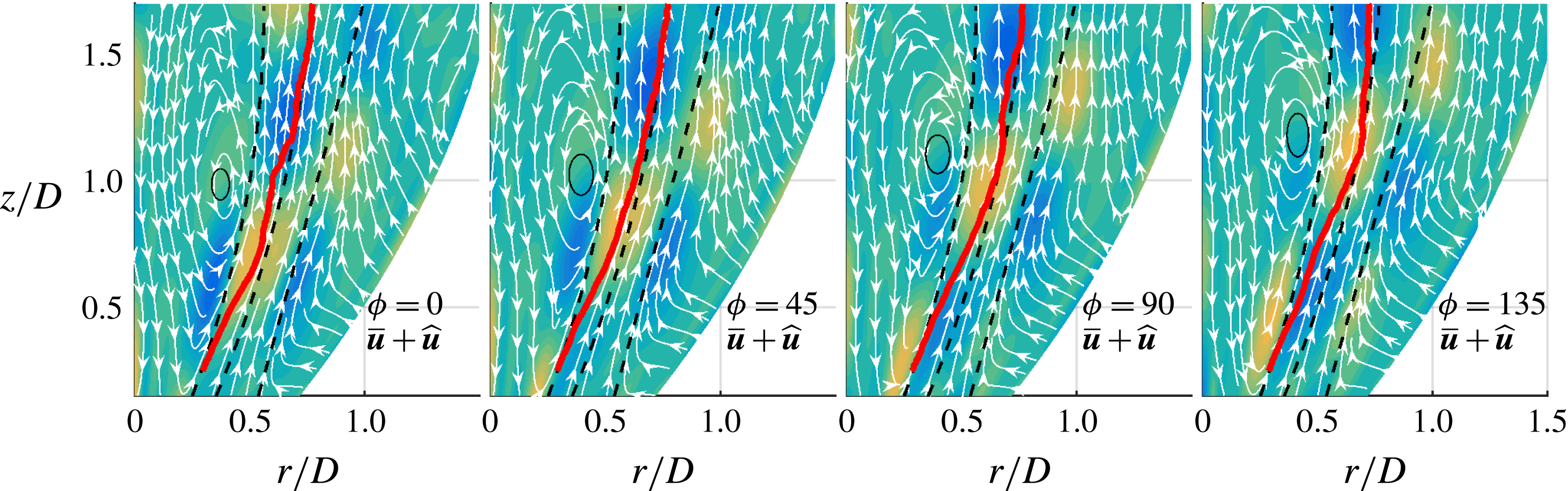
Having shown the dominant features of the forced flame and flow, we next consider the spatial structure in more detail. Figure 19 shows the phase-reconstructed (defined as the sum of the time-averaged component and component characterization of forced response oscillating at the forcing frequency) velocity field streamlines overlaid on the phase-reconstructed vorticity disturbance field for the 390 Hz IP forcing case. The phase reconstruction shown here uses the sum of helical coefficients for calculating the disturbance. Were only the
 $m=0$
disturbance used, there would be little observable difference, because the other modes are negligible in comparison, as demonstrated by figure 16. The phase-reconstructed vorticity disturbance fields show convective disturbances with a wavelength of approximately
 $0.5D$
. Three vortical disturbance peaks are evident – one inside the ISL, one along the JC and one outside of the OSL. As these vortical disturbances convect downstream, they are damped and amplified separately. For example, while the innermost disturbance has decayed in amplitude by
 $z/D=1$
, the middle disturbance along the JC continues to grow in strength.
It should also be noted that these vortical disturbances are distinct from the large region of rotating flow just inside the ISL that is shown by the full (i.e. sum of the time averaged and disturbance) flow field. Because the vortical disturbances in this particular case are weak compared to the time-averaged vorticity, they do not appear within the phase-reconstructed field as clear regions of rotation in the streamline. Instead, they act to capture the weak convective motion of the centre of the large region of rotation. The phase-averaged flame edge, beginning in the shear layer and moving into the jet, is periodically deformed by the vortical disturbance field. While the disturbances may be small in magnitude, they have a significant effect on heat release as they are axisymmetric (Smith et al. Reference Smith, Emerson, Proscia and Lieuwen2018).
The 390 Hz IP phase-reconstructed flow field (superposition of time averaged velocity field and phase averaged velocity disturbance field at the forcing frequency) overlaid on the vorticity disturbance field. Black dashed lines are the ISL, JC and OSL, and the red line is the ensemble-averaged flame edge.

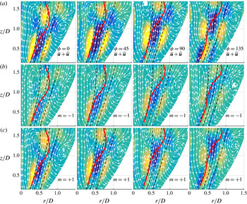
(a) The 390 Hz OP phase-reconstructed flow field and flame position overlaid on the vorticity disturbance field. (b,c) Same data but only using
 $m=+1$
or
 $m=-1$
mode for reconstruction to show their separate contribution to the overall velocity shown in the top figure. Black dashed lines are the ISL, JC and OSL, and the red line is the ensemble-averaged flame edge.

Similarly, figure 20 shows the phase-reconstructed velocity fields for the 390 Hz OP forcing case with the phase-averaged flame edge overlaid. Figure 20(a) shows the velocity field reconstructed using the mean and the sum of the helical mode coefficients while the bottom two rows use only the
 $m=-1$
and
 $m=+1$
coefficients for the disturbance. The flame edge on each plot is the total disturbance, as it has not been decomposed. These two modes are analysed individually as figure 18 suggests that the dominant energy modes are in both the
 $m=\pm 1$
modes. This figure shows that at low axial distances (
 $z/D<0.6$
), both disturbances are of near equal amplitude, as shown by the colour. While both modes grow axially, the
 $m=+1$
mode becomes stronger than the
 $m=-1$
mode. This shows that while the acoustics may excite the two modes nearly equally at the nozzle outlet, the flow field preferentially amplifies the
 $m=+1$
mode. Additionally this shows that the growth of the
 $m=+1$
mode does not occur at the expense of the
 $m=-1$
mode, showing that the two modes co-exist and that one mode does not necessarily suppress the other. Additionally the convection of the disturbances in the positive axial direction gives a positive
 $k$
value (see (1.1)) and means that the co-rotating
 $m=+1$
mode is counter-winding while the counter-rotating
 $m=-1$
mode is co-winding; see figure 2 for a visualization of these modes.
Superposing the phase-averaged flame edge on the flow field adds insight into the velocity–flame interaction. At low axial heights the flame shows very little disturbance; however, as the flow field disturbance amplitudes grow, the flame disturbance amplitude also grows and becomes noticeable beyond
 $z/D=0.5$
. The phase-averaged flame edge reaches the JC around an axial distance of
 $z/D=0.8$
which corresponds with the location of maximum disturbance amplitude in the JC. This large flapping motion does not occur for the IP forcing case as the amplitude of the radial disturbances are weaker than the OP case. Additionally, the IP case forces an acoustic velocity node near the centreline, so the acoustic disturbance also does not aid in the flame propagation across the JC.
Analysing the IP forcing field showed that the superposition of the
 $m=0$
mode on the time-averaged field resulted in convection of the region of rotation within the ISL and caused a small oscillatory expansion of the annular jet. The weak disturbances for this particular case meant that there were no large motions on the phase-reconstructed field. The OP forcing, however, experienced much stronger disturbances that were able to effect the phase-reconstructed flow field. The comparison of the
 $m=\pm 1$
disturbance fields resulting from OP forcing shows that the
 $m=\pm 1$
modes grow together, with the co-rotating
 $m=+1$
mode preferentially amplified.
4.3 Axial evolution of disturbance modes
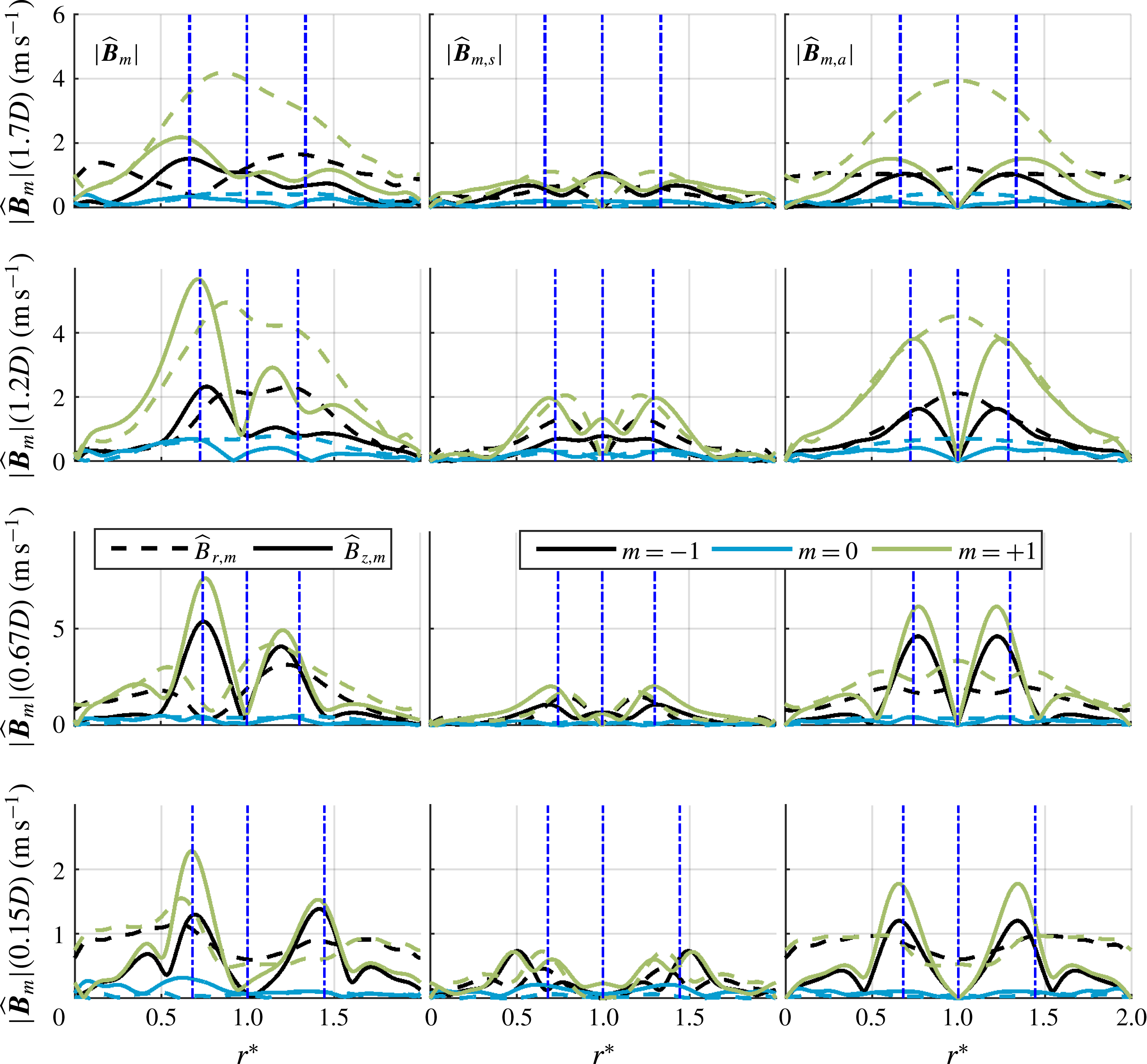
This section further considers the relative amplitude and axial evolution of the hydrodynamic modes, using the symmetric–anti-symmetric decomposition of (3.5). Figure 21 shows the decomposition of the interpolated helical modes at multiple axial locations for the IP case. As noted before, the forced
 $m=0$
mode is dominant throughout the flow field. Figure 21 also shows that, at the lowest height,
 $z/D=0.15$
, the symmetric axial mode is strong throughout the jet. This is very likely a manifestation of bulk axial acoustic disturbances (as discussed in § 3.1, no acoustic subtraction was attempted for the IP case), while the anti-symmetric axial disturbances are dominated by vortical disturbances in this region. The vortical disturbances shown in figure 19 necessarily ignore this acoustic contribution. As the flow convects downstream, the anti-symmetric axial and radial disturbances grow in peak amplitude and spread out radially with the widening shear layer. The growing radial anti-symmetric disturbance is due to dilatational disturbances caused by the flame motion, while the spreading of the radial and axial modes is due to phase jitter. This shows that the transverse pressure anti-node results in negligible oscillating mass fluctuations through the nozzle. Additionally the figure shows that the co-rotating, counter-winding
 $m=+1$
mode and counter-rotating, co-winding
 $m=-1$
modes grow downstream despite being negligible in amplitude near the nozzle exit. The flow amplifies both of these modes, particularly the co-rotating, counter-winding
 $m=+1$
mode which peaks around
 $z/D=0.7$
.
Helical mode profiles and decomposition about the JC for both axial (solid) and radial (dashed) velocity components for the 390 Hz IP forcing case. JC, ISL and OSL lines (dash-dot) are shown for reference.

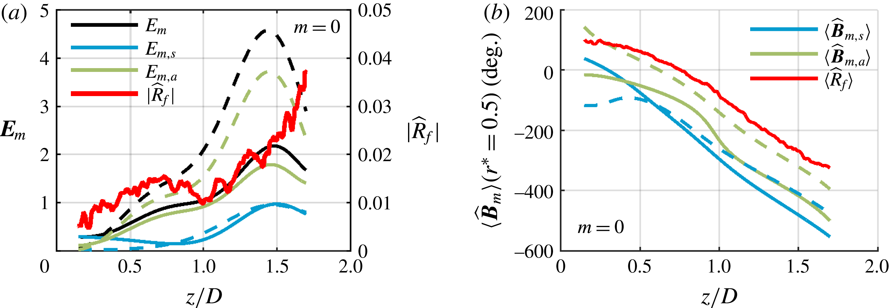
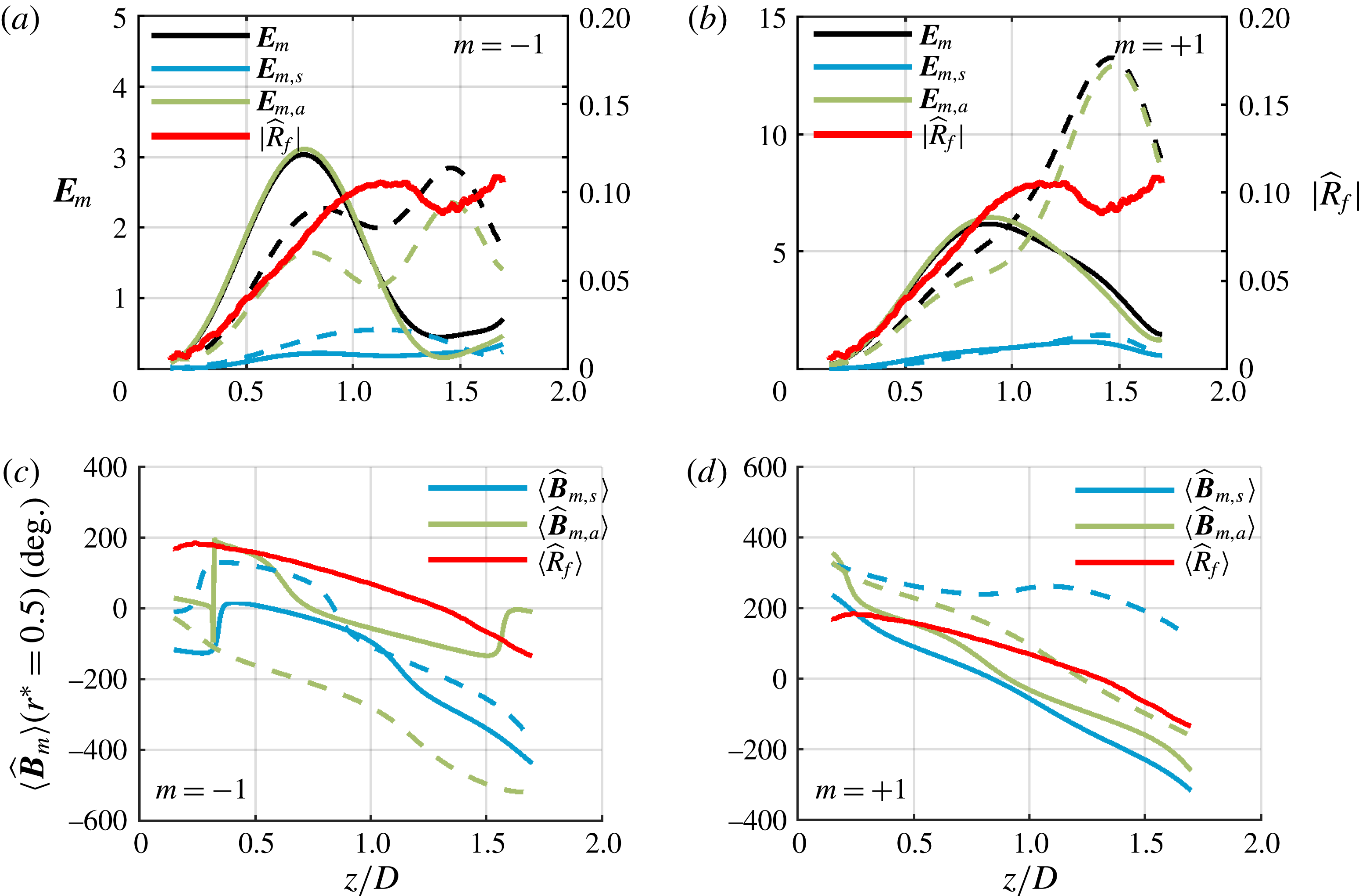
Figure 22 plots the radially integrated energy of the
 $m=0$
mode over the decomposition domain,
 $\boldsymbol{E}_{m}=\int |\hat{\boldsymbol{B}}_{m}|^{2}r\,\text{d}r$
. The black line represents the total energy of the interpolated mode shape, the blue line represents the integrated energy of the symmetric mode and the green line represents the integrated energy of the anti-symmetric mode. It is clear from this plot that the
 $m=0$
mode is dominated by the combination of the axial and radial anti-symmetric modes about the JC. It is expected that the most dominant radial mode is anti-symmetric as the acoustic excitation results in a transverse anti-symmetric disturbance about the JC. Additionally, the peak of this mode occurs at
 $z/D=1.4$
, which coincides with where the jet stops expanding and where the recirculation zone begins to close. The axial phase taken at a single normalized radius shows a constant convection speed for the dominant anti-symmetric modes – the slope of these lines correspond to a disturbance convection speed of
 $14.6~\text{m}~\text{s}^{-1}$
. Additionally the radial and axial anti-symmetric modes act approximately
 $90^{\circ }$
out of phase with each other, and the phase of the flame envelope follows the
 $m=0$
modes quite well.
The flame edge envelope is also shown. The envelope grows initially with the disturbances, then deviates near an axial distance of
 $z/D=0.7$
. This is due to the weak
 $m=0$
perturbations experienced by the flame and to interference effects from the other helical modes.
(a) Radial integration of total energy, symmetric mode energy and anti-symmetric energy for both axial (solid) and radial (dashed) velocity components for the 390 Hz IP
 $m=0$
mode with the flame envelope and (b) the corresponding phase plots of the decomposition maintaining the original phase reference.

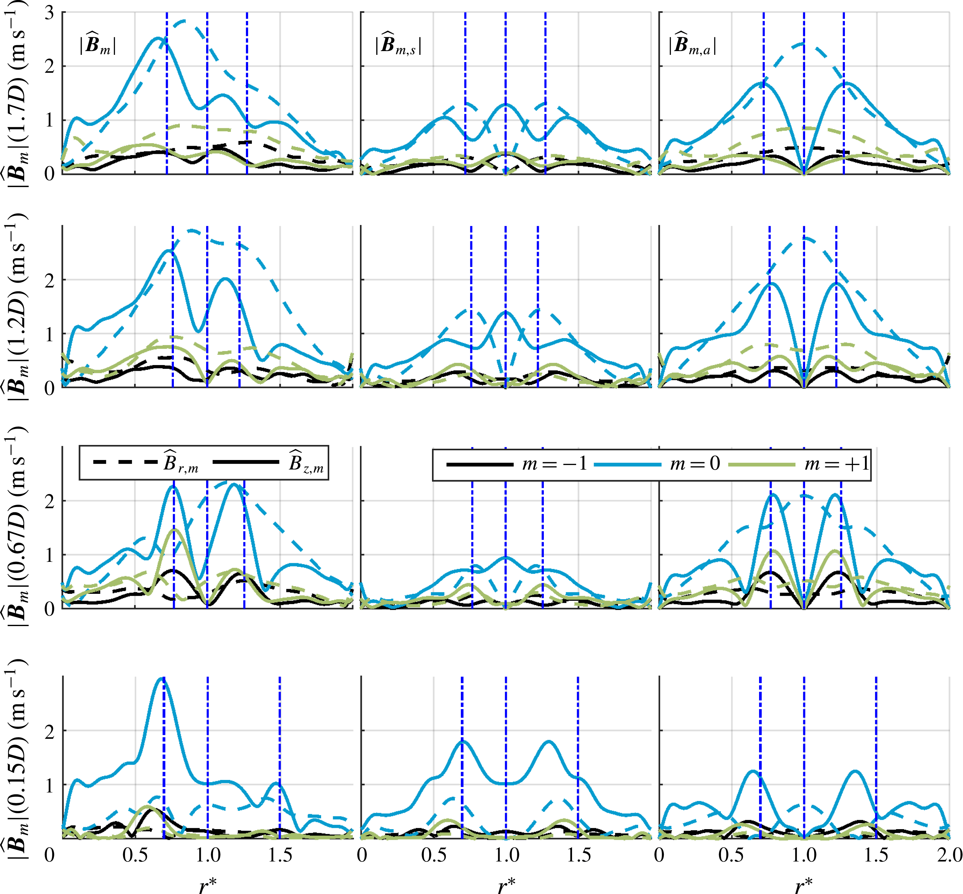
Figure 23 shows the spatial decomposition of the interpolated helical modes for the 390 Hz OP forcing case. The axial disturbances are strongly anti-symmetric and located in the shear layers, while the radial disturbances are dominated by anti-symmetric disturbances throughout the entire jet. This combination for the
 $m=\pm 1$
modes represents the precession of the annular jet about the geometric centre of the flow field. When the two precession motions are of equal amplitude, the superposition of the two results in the side-to-side flapping of the jet. However, at further downstream locations, the
 $m=+1$
anti-symmetric mode becomes dominant. This shows that the motion of the annular jet transitions from a flapping motion to a precession motion in the swirl direction. Additionally, note that at further downstream locations, the axial disturbances lose their sharpness and amplitude due to the combination of phase jitter and amplitude decay while the radial disturbances continue to grow. This growth in the radial structure is due to the dilatational disturbance created by the flapping flame. Consistent with this trend, figure 24 shows that the energy of the anti-symmetric radial mode is constantly growing throughout most of the domain and peaks near the downstream end of the domain.
Interpolated helical mode profiles and decomposition about the JC for both axial (solid) and radial (dashed) velocity components for the 390 Hz OP forcing case. JC, ISL and OSL lines (dash-dot) are shown for reference.

Figure 24 shows the radially integrated data for the OP forcing case. First, note the difference in mode envelopes between the axial and radial velocity components: the radial envelope shows a bimodal structure peaking around
 $z/D=0.8$
and
 $z/D=1.5$
while the axial profile only peaks around
 $z/D=0.8$
. This is because the axial fluctuations and axial velocity are decaying as they progress downstream while the transverse modes are switching from a vortical disturbance to a strong dilatational disturbance due to the flame flapping. The flame edge fluctuations grow, following the
 $m=+1$
radial fluctuations, and reach a near maximum around
 $z/D=1.1$
where the flame crosses the jet periodically. As mentioned earlier, the flame moves out of the inner shear layer around
 $z/D=0.8$
, corresponding to the peak axial fluctuation and suggesting that the axial fluctuations are tied to baroclinic torque provided by the density stratification of the flame. Additionally, the phase plots show that the anti-symmetric axial and radial modes are approximately
 $90^{\circ }$
out of phase with each other, which is expected for the motion this decomposition describes. The energy in the symmetric modes is primarily a result of the fit to the spatial noise not captured by the anti-symmetric component, therefore its phase plots do not look coherent. Note that the phase speed of the flame edge fluctuations tends to match the
 $m=-1$
modes better than the
 $m=+1$
modes despite the
 $m=+1$
mode being dominant.
Radial integration of total energy, symmetric mode energy and anti-symmetric energy for both axial (solid) and radial (dashed) velocity components for the 390 Hz OP (a)
 $m=-1$
and (b)
 $m=+1$
modes with the flame envelope and the corresponding phase plots of the decomposition maintaining the original phase reference for (c)
 $m=-1$
and (d)
 $m=+1$
.

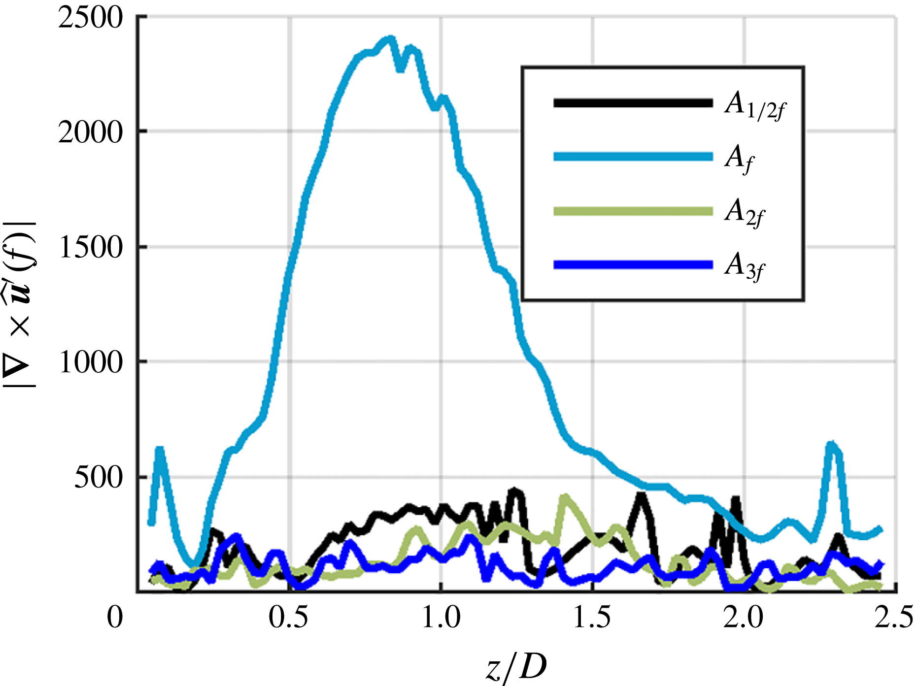
The above data all show growth, followed by decay of the disturbance modes. An important question to address is the relative role of linear and nonlinear processes in leading to the saturation and decay of these disturbances. Next, we briefly consider the significance of nonlinear effects. Self-excited global modes are characterized by narrowband instabilities that grow in time until linear and nonlinear dissipation balance growth, resulting in limit-cycle oscillations. On the other hand, forced modes can derive energy from external forcing and need not rely on temporal feedback for growth, instead extracting energy from the forcing in some region and developing spatially as the flow convects away. This allows forced modes to exhibit linear spatial growth, so long as the amplitude of the oscillation remains small enough for nonlinear effects to be insignificant (which may not be true for all of the domain). A key signature of nonlinear effects is the presence of harmonics and/or subharmonics of the forcing frequency. Figure 25 shows the envelopes of vorticity disturbances along the JC taken from the
 $r$
–
 $z$
plane Fourier coefficients,
 $\hat{\boldsymbol{u}}^{\prime }$
, at the forcing frequency and its first two harmonics. These results were obtained from the 390 Hz OP forcing case as it shows the larger response amplitude and should, therefore, exhibit the largest nonlinear effects. This JC line was selected because the line of maximum amplitude disturbances at the forcing frequency passes through the JC. Figure 25 clearly shows that there is a strong response at the forcing frequency,
 $A_{f}$
, and a minimal response at the subharmonic,
 $A_{1/2f}$
and harmonics,
 $A_{2f}$
and
 $A_{3f}$
, which falls into the noise level of the spectra at each axial location. These results strongly suggest that nonlinearities do not play an important role in controlling the flow dynamics for these reported cases.
Envelope of vorticity disturbance amplitude along the left side JC for the 390 Hz OP case, taken directly from un-interpolated
 $r$
–
 $z$
data for the forcing frequency and its harmonics.

We close this section by summarizing a few key observations and reflecting on how they compare with stability predictions and prior studies. As noted, the
 $m=+1$
, co-rotating, counter-winding mode grows more rapidly than the
 $m=-1$
, counter-rotating, co-winding mode. Although the acoustic forcing excites both modes at the nozzle outlet equally, the co-rotating mode is apparently more strongly amplified as it convects along the flow. As argued above, there is little evidence of significant nonlinear effects, and so this preferential amplification appears to be a linear effect – i.e. that the spatial growth rate of the
 $m=+1$
mode is larger than that of the
 $m=-1$
mode. Moreover, this difference clearly must be due to an asymmetry induced by swirl. Some insight into this result can be obtained from linear stability analysis (Howard & Gupta Reference Howard and Gupta1962; Wang et al.
Reference Wang, Rusak, Gong and Liu2016). In particular, it is known that an upper bound can be established for the temporal growth rate of an arbitrary helical disturbance in constant-density inviscid columnar vortices (see equation (22) in Howard & Gupta (Reference Howard and Gupta1962)). Application of this result shows that a counter-winding disturbance may always have a higher temporal growth rate than a co-winding disturbance in the inner shear layer where the radial gradient of the axial velocity is positive, with the opposite holding true in the outer shear layer. Among other things, mean swirl reduces the effective shear for disturbances winding in the same direction as the swirl. While this result applies to temporal growth rates, application of Gasters’ transformation (Gaster Reference Gaster1962) (reasonable to do, considering the lack of any observed natural narrowband fluctuations, see figure 4), implies that the spatial growth rate may also favour counter-winding disturbances in the inner shear layer.
Next, little evidence of strong nonlinear effects, at least as manifested in the presence of subharmonics or harmonics of the forcing frequency, were observed in these data, even though the disturbances achieved quite significant amplitudes relative to the mean axial velocity at the nozzle exit – of the order of 5 % near the nozzle exit and peaking at values close to 25 %. Nonlinear modal interactions have been studied extensively in non-swirling jets, and have been shown to produce subharmonic resonant interactions which, when excited, modify both the mean flow and the observed dynamics (Cohen & Wygnanski Reference Cohen and Wygnanski1987). However, such interactions require similar disturbance phase speeds to allow time for nonlinear energy transfer mechanisms to act. In axisymmetric non-swirling jets, this condition is met by degenerate helical modes rotating in opposite directions, which propagate at the same phase speeds and produce a standing wave-like interference pattern (Long & Petersen Reference Long and Petersen1992). However, as mentioned earlier, the introduction of swirl breaks this symmetry, and thereby requires interactions among non-degenerate modes with different phase speeds. This all suggests that a convectively unstable hydrodynamic mode concentrated within the ISL and receptive to the forcing frequency is causing a preferential linear amplification of counter-winding modes, which in this facility corresponds to the
 $m=+1$
disturbances, who exhibit little downstream interaction, at least as manifested by the presence of harmonics or subharmonics.
Finally, a related point worth highlighting is the fact that forced flows of this nature, at least for amplitudes and/or spatial regimes where the dynamics is linear, can exhibit multiple hydrodynamic modes at the same time, In agreement with other studies of swirling jets (Liang & Maxworthy Reference Liang and Maxworthy2005; Oberleithner et al. Reference Oberleithner, Sieber, Nayeri, Paschereit, Petz, Hege, Noack and Wygnanski2011; Rukes et al. Reference Rukes, Sieber, Paschereit and Oberleithner2016). These modes can include both co- and counter-winding helical modes, as well as symmetric and anti-symmetric jet column disturbances. In contrast, unforced but globally unstable systems, where the limit-cycle motion is a clear indication of strong nonlinear effects, appear to be dominated by a single mode (Billant et al. Reference Billant, Chomaz and Huerre1998; Liang & Maxworthy Reference Liang and Maxworthy2005) possibly due to saturation.
5 Conclusions
This paper has shown how phase locked results from multi-plane (both
 $r$
–
 $z$
and
 $r$
–
 $\unicode[STIX]{x1D703}$
) measurements can be combined to elucidate the three-dimensional disturbance structure of a forced, swirling, reacting jet. In particular, using a volumetric interpolation approach, the velocity and vorticity fields were decomposed into their various azimuthal modes, and the azimuthal modes were decomposed into symmetric and anti-symmetric disturbances about the jet core. Given that the overall velocity field is a superposition of modes with different azimuthal periodicities, and jet core symmetries, such a decomposition lends considerable additional insight into the velocity field than can be obtained by looking at a single plane.
Measurements showed that the dominant forced helical modes could be qualitatively predicted with forcing function expressions derived by O’Connor et al. (Reference O’Connor, Acharya and Lieuwen2015). However, these modes can evolve axially in a quite different manner, particularly for the OP forcing case where the
 $m=\pm 1$
modes start at near equal amplitude but soon diverge as the co-rotating, counter-winding
 $m=+1$
mode is preferentially amplified. The counter-rotating, co-winding
 $m=-1$
mode is still significant, but does not interact with the co-rotating mode. This makes the flow and flame transition from a transverse flapping motion to a precessing motion at further downstream distances. It was hypothesized that the
 $m=+1$
mode was preferentially amplified because it was counter-winding, based upon some results from temporal stability theory. As for the IP forcing case, the axisymmetric
 $m=0$
modes dominated throughout the entire flow field, as this mode was the most strongly excited. The presence of the
 $m=\pm 1$
modes were also detected, but their effect on the flow field was minimal in comparison to the
 $m=0$
mode. Additionally, the symmetric/anti-symmetric decomposition of the flow field shows that the motions in the shear layers that are anti-symmetric or sinuous about the jet core are most amplified; these are the modes associated with transverse motions of the annular jet. This trend holds for all azimuthal modes for the given transverse forcing cases which raises the question of whether axial forcing would also see this same trend.
Several questions emerge from this work for future studies. First, while the flow dynamics appears to remain linear here, it will be of interest to study this configuration over a larger range of forcing amplitudes where strong nonlinearities arise. This raises the questions of if and how nonlinear competition between symmetric and asymmetric modes, co- and counter-rotating modes, or co- or counter-winding modes arise. For example, would one of the modes, say the
 $m=-1$
be completely eliminated in favour of another mode? A related study of interest would be excitation of additional modes; for example, by exciting the
 $m=-1$
,
 $m=0$
and
 $m=+1$
modes with comparable amplitude (which can be done with a travelling acoustic wave, rather than a standing wave). In addition, exciting other even modes with significant amplitudes, such as
 $|m|=2$
, will be of interest, to see how axisymmetric and helical disturbances interact, as well as even and odd modes.
One of the key challenges with measurements of this nature is handling the large volumes of data that are acquired; indeed, transferring data from cameras is one of the main time requirements for the experimental campaigns, and camera memory generally limits the size of data records. While the data acquired here were sufficient to elucidate to high precision key spectral characteristics, the ability to transfer and manipulate much larger data sets will also enable answering additional questions. For example, one interesting question is the degree of interaction between the different modes – as they undergo inherent stochastic disturbances in vortex core location, are their motions phase locked to each other or do they evolve completely independently? This question can be addressed by determining the coherence between these quantities, whose meaningful estimate would require roughly an order of magnitude longer time series. In addition, returning to the nonlinear interactions question, longer data sets will be required to analyse higher-order nonlinear correlations (e.g. the degree of interaction for the
 $m=+1$
mode at
 $\unicode[STIX]{x1D714}$
and the
 $m=1$
mode at
 $2\unicode[STIX]{x1D714}$
), such as the bispectrum.
These studies motivate additional theoretical studies as well. In particular, while the
 $m=+1$
mode was preferentially amplified, it would be of interest to analyse the relative roles of shear, centrifugal instabilities, baroclinic torque and dilatation in controlling these results. Such a study could also assess the sensitivity of these results to small variations in, say, relative locations of the shear layer and flame which strongly influences how induced baroclinic vorticity interacts with shear-generated vorticity. Related questions arise for the forced response of a flow, and how the different shear, rotation and gas expansion terms influence the relative growth rates of different types of modes, and at different frequencies.
Acknowledgements
This research was partially supported by the Air Force Office of Scientific Research under award no. FA9550-16-1-0442, contract monitor Dr C. Li. Additionally the authors would like to thank J. Lim and A. P. Naidu for their aid in the experimental aspect of this paper.