1. Introduction
New developments in the problem of the detection of extreme events have resulted in a considerable interest in the determination of statistical properties of time series of the surface elevation. Traditionally, in such an analysis the key parameter to express the severity of the sea state has been the wave height, which for a single wave is defined as the distance between the trough and the crest of the wave. As typically many waves with different frequency and direction are present a statistical approach is usually followed. In practice, researchers obtain the wave height distribution by means of the zero-crossing method. This is a very elegant method, which is easily implemented. One just searches for two consecutive zero-upcrossings in the time series and one determines the wave height from the difference of the maximum and the minimum of the surface elevation
 ${\it\eta}$
in the corresponding time interval. Thus, wave height is determined by sampling with the zero-crossing frequency given by
 $(m_{2}/m_{0})^{1/2}$
(with
 $m_{n}$
the
 $n$
th moment of the wave spectrum), and to quantify the severity of the sea state one determines the probability distribution function (p.d.f.) of wave height. By applying the zero-crossing method to observed time series of the surface elevation it turns out that the resulting p.d.f. depends on spectral shape. For a narrow-band spectrum the wave height p.d.f. is found to be close to the Rayleigh distribution, in agreement with theoretical results by Longuet-Higgins (Reference Longuet-Higgins1957), while for broad-banded spectra extreme waves are, when compared to the Rayleigh distribution, less likely to occur. The underestimation of the probability of extreme events for broad-banded spectra is problematic as will discussed below.
While for narrow-band spectra it can be shown that the wave height distribution is indeed a Rayleigh distribution, for broad-banded spectra the theoretical wave height p.d.f. is, as far as I know, not known. This therefore presents a stumbling block when one is interested in the development and verification of a theory for extreme events for arbitrary spectra. This led me to consider alternative ways to measure the intensity of extreme events. A prominent candidate is to use instead of wave height the envelope of a wave train. This idea, which was probably first suggested by Gabor (Reference Gabor1946) in the field of signal processing, has been proposed by a number of authors in the field of ocean waves as well. Examples include the work of Naess (Reference Naess1982), Shum & Melville (Reference Shum and Melville1984) and, although restricted to narrow-band wave trains, the work of Tayfun & Lo (Reference Tayfun and Lo1990).
The choice of using the envelope of the signal has a number of advantages. First, for a Gaussian sea state it will be shown in this paper that the p.d.f. of the envelope height is always Rayleigh, independent of spectral shape. Second, in actual applications it is important to determine extreme forces on structures such as oil rigs or ships. An interesting quantity to know then is the energy of the waves. The square of the envelope is a measure for the potential energy of the wave train and is therefore closely related to the wave energy. On the other hand, for extreme cases the square of the wave height would underestimate, for broad-banded spectra, the forces on structures as the p.d.f. of wave height falls below the Rayleigh distribution by a significant amount while the envelope p.d.f. is Rayleigh.
Another advantage of the use of the envelope is that it is fairly easy to construct from a time series at any point in time, but this is not really possible if wave height is obtained from the zero-crossing method as wave height will be sampled in a discrete manner with the zero-crossing frequency. As the envelope is a continuous function in time its p.d.f. may be made as accurate as possible by simply sampling at a sufficiently high frequency. In other words, there is a definite case to be made to concentrate on the envelope distribution rather than the wave height distribution.
In this paper I will obtain the joint probability of wave height and period starting from the idea that the envelope of a wave train gives an adequate characterization of the severity of the sea state. The time series will therefore be given in terms of an envelope function
 ${\it\rho}$
and a local phase
 ${\it\phi}$
. Here, wave height will be defined as twice the envelope height while the local frequency will be given by
 ${\it\omega}=-\partial {\it\phi}/\partial t$
. It is then important to have a procedure to obtain from the time series of
 ${\it\eta}(t)$
the envelope and the phase of the wave train. Two methods have been explored. The first one, described in § 2, assumes that
 ${\it\eta}(t)$
is an analytic signal so that envelope and phase may be obtained from the signal
 ${\it\eta}$
and its orthogonal complement, the Hilbert transform. This is a well-known method, already applied by Shum & Melville (Reference Shum and Melville1984) to observed time series of ocean waves. The second method assumes that the correlation
 $R({\it\tau})=\langle {\it\eta}(t){\it\eta}(t+{\it\tau})\rangle$
has at least one zero at
 ${\it\tau}={\it\tau}_{\ast }$
. Then,
 ${\it\eta}(t)$
and
 ${\it\eta}(t+{\it\tau}_{\ast })$
are orthogonal and may be used to obtain the envelope and phase of the wave train.
In § 3 it is shown that the reduction of a complicated signal to just two parameters, namely envelope and frequency, will provide useful information on the statistical properties of the time series for surface elevation. For Gaussian signals with a stationary two-point correlation function it will be shown that there is excellent agreement between the theoretical joint p.d.f. of envelope wave height and period and the corresponding p.d.f. obtained from Monte Carlo simulations of the (analytic) signal. This good agreement is not only obtained for narrow-band spectra but also for broad-band spectra. The present approach is therefore an extension of the work of Longuet-Higgins (Reference Longuet-Higgins1983) and Xu et al. (Reference Xu, Li, Zhang, Xu and Lu2004) and, as discussed in § 4, is therefore a good starting point for the development of a statistical theory of weakly nonlinear waves. Finally, in § 5 a summary of conclusions is presented.
2. Joint distribution of envelope height and period
Before developing the theory for the joint p.d.f. of envelope height and period we first have to make some underlying assumptions more explicit. In the field of ocean waves a central role is given to the energy balance equation which describes the evolution in space and time of the wave variance spectrum. The energy balance equation has been derived under the assumption that the waves are weakly nonlinear, that the wavefield may be regarded as homogeneous and stationary while the probability distribution of the ocean surface elevation is approximately Gaussian. The same assumptions will be used in the determination of the joint p.d.f. of envelope wave height and period, in particular for evaluating the connection between certain correlations and the wave spectrum. Here, the wave spectrum follows from the Fourier transform of the two-point correlation function
 ${\it\rho}$
defined as
 $$\begin{eqnarray}{\it\rho}({\it\tau})=\langle {\it\eta}(t){\it\eta}(t+{\it\tau})\rangle ,\end{eqnarray}$$
and for stationary conditions the correlation function only depends on the time difference
 ${\it\tau}$
. The angular frequency spectrum
 $E({\it\omega})$
is then given by
 $$\begin{eqnarray}E({\it\omega})=\frac{1}{2{\rm\pi}}\int \text{d}{\it\tau}{\it\rho}({\it\tau})\cos ({\it\omega}{\it\tau}),\end{eqnarray}$$
and, in particular, the moments of the wave spectrum are important for knowledge of the statistical properties of the time series.
In order to obtain the joint p.d.f. of envelope and period a method is required to obtain from a given time series
 ${\it\eta}(t)$
the envelope
 ${\it\rho}$
and local phase
 ${\it\phi}$
. In fact, as will be seen in this paper, several procedures are possible. Here, we start by assuming that the time series is analytic and we follow the work of Gabor (Reference Gabor1946) closely.
Let us restrict our attention to analytic functions
 $Z(t)={\it\eta}+\text{i}{\it\zeta}$
. These functions have the remarkable property that if the real part of
 $Z$
is known then the imaginary part of
 $Z$
is given by the Hilbert transform of its real part. Thus,
 $$\begin{eqnarray}{\it\zeta}=\text{Im}(Z)=\pm H({\it\eta})=\pm \frac{1}{{\rm\pi}}\int \text{d}{\it\tau}\frac{{\it\eta}({\it\tau})}{t-{\it\tau}},\end{eqnarray}$$
where the integral is a principal value integral and the
 $\pm$
sign depends on the chosen assumed behaviour of the complex function
 $Z$
for large arguments (cf. the Remarks below). Envelope
 ${\it\rho}$
and phase
 ${\it\phi}$
are now defined as
 $$\begin{eqnarray}{\it\rho}\;\text{e}^{\text{i}{\it\phi}}=Z(t)={\it\eta}+\text{i}{\it\zeta},\end{eqnarray}$$
therefore
 $$\begin{eqnarray}{\it\eta}={\it\rho}\cos {\it\phi},\quad {\it\zeta}={\it\rho}\sin {\it\phi}.\end{eqnarray}$$
Envelope and phase follow now at once from
 ${\it\eta}$
and
 ${\it\zeta}$
,
 $$\begin{eqnarray}{\it\rho}=\sqrt{{\it\eta}^{2}+{\it\zeta}^{2}},\quad {\it\phi}=\arctan ({\it\zeta}/{\it\eta}).\end{eqnarray}$$
In this fashion (and this is of course very well-known) one may obtain from a real time series the envelope and phase of a wave train. This is a very general approach. For a narrow-band wave train (but note that we will not make this assumption here)
 ${\it\rho}$
and the derivative of
 ${\it\phi}$
will be slowly varying functions in time and space. In those circumstances it is customary to introduce the local angular frequency through
 $$\begin{eqnarray}{\it\omega}=-\frac{\partial {\it\phi}}{\partial t},\end{eqnarray}$$
and for a narrow-band wave train the local frequency is also slowly varying. The key point is now that we generalize the notion of a local frequency by also applying the same definitions for a wave train with a broad-banded spectrum. Hence, for any time series
 ${\it\eta}$
we obtain envelope and phase from (2.6) where
 ${\it\zeta}$
is the Hilbert transform of
 ${\it\eta}$
. The joint p.d.f. of envelope
 ${\it\rho}$
and period
 $T$
is then easily obtained by making use of the local frequency
 ${\it\omega}$
of (2.7) and the definition
 $T=2{\rm\pi}/{\it\omega}$
.
Remarks on the procedure. It is indeed a remarkable result that one may construct a complex signal
 $Z$
from its real part and the Hilbert transform of its real part, but there is also a caveat. A unique solution can only be found provided one makes an assumption regarding the behaviour of the complex function
 $Z(z)$
for large complex
 $z$
.
Is it possible to find for given function
 $g(x)$
on the real axis a unique analytical function
 $f(z)=g(z)+\text{i}h(z)$
, with
 $z=x+\text{i}y$
? This is simply not possible unless some conditions on the behaviour of
 $f(z)$
for large
 $z$
are imposed. To illustrate the point consider the function
 $g(x)=\cos x$
. There are at least two complex functions
 $f(z)$
that give the same function on the real axis, namely
 $f(z)=\exp (\text{i}z)$
and
 $f(z)=\exp (-\text{i}z)$
. So the solution is not unique unless one imposes an additional condition on the behaviour of
 $f(z)$
. Imposing the condition that
 $f(\text{i}y)$
vanishes sufficiently rapidly for
 $y\rightarrow \infty$
will give rise to the unique solution
 $f(z)=\exp (\text{i}z)$
, while the condition that
 $f(\text{i}y)$
will vanish sufficiently rapidly for
 $y\rightarrow -\infty$
will give rise to the second solution
 $f(z)=\exp (-\text{i}z)$
.
This has consequences for the extension of a real signal into the complex domain. If
 $f(z)$
is analytic and
 $C$
is a piecewise smooth closed contour in an open domain, then according to the Cauchy integral theorem
 $$\begin{eqnarray}\int _{C}\frac{f(z)}{z-z_{0}}\text{d}z=2{\rm\pi}\text{i}f(z_{0}),\end{eqnarray}$$
if
 $z_{0}$
is inside
 $C$
. If
 $z_{0}$
is outside
 $C$
then the singular integral vanishes.
The result in (2.3) now follows by making a special choice of the contour
 $C$
. Consider a contour
 $C$
that consists of a semicircle
 ${\it\Gamma}_{R}$
with radius
 $R$
and the real axis from
 $-R$
to
 $+R$
, hence
 $C={\it\Gamma}_{R}+[-R,R]$
. First suppose that
 $f(z)$
vanishes sufficiently rapidly for
 $y\rightarrow \infty$
so that the contribution from the semicircle in the upper half-plane,
 ${\it\Gamma}_{R}^{u}$
, vanishes. In the limit
 $R\rightarrow \infty$
one then finds
 $$\begin{eqnarray}P\int _{-\infty }^{\infty }\frac{f(x)}{x-x_{0}}\text{d}x={\rm\pi}\text{i}\,f(x_{0}).\end{eqnarray}$$
Writing
 $f(x_{0})=g(x_{0})+\text{i}h(x_{0})$
one immediately finds from the real part of the above equation that
 $$\begin{eqnarray}h(x_{0})=\frac{1}{{\rm\pi}}P\int _{-\infty }^{\infty }\frac{g(x)}{x_{0}-x}\text{d}x,\end{eqnarray}$$
corresponding to the
 $+$
sign result of (2.3).
However, if one now assumes on the other hand that
 $f(z)$
vanishes sufficiently rapidly for
 $y\rightarrow -\infty$
then in order that the contribution along the semicircle vanishes one has to close the contour
 $C$
by choosing a semicircle
 ${\it\Gamma}_{R}^{l}$
in the lower half-plane. The end result has a different sign. Therefore the extension of a real function into the complex plane is not unique, and results will depend on assumptions regarding the behaviour of the complex function for large
 $z$
.
Finally, in this paper the starting point is the complex function
 $Z$
(see for example § 2 and appendix A) so the behaviour at large
 $z$
is known. Following the above procedure the sign in (2.3) is therefore known so that there is no ambiguity.
In order to obtain the joint p.d.f. of envelope and period we follow the work of Longuet-Higgins (Reference Longuet-Higgins1983), see also Xu et al. (Reference Xu, Li, Zhang, Xu and Lu2004). The starting point is the assumption that
 ${\it\eta}(t)$
is a stationary Gaussian process. Since
 $\dot{{\it\eta}}$
,
 ${\it\zeta}$
and
 $\dot{{\it\zeta}}$
are linear transforms of
 ${\it\eta}$
their joint p.d.f. is Gaussian and therefore can be expressed as
 $$\begin{eqnarray}p(\boldsymbol{x})=\frac{1}{(2{\rm\pi})^{2}|{\it\bf\Sigma}|^{1/2}}\exp \left\{-\frac{1}{2}\boldsymbol{x}^{\text{T}}{\it\bf\Sigma}^{-1}\boldsymbol{x}\!\right\},\end{eqnarray}$$
where
 $\boldsymbol{x}=({\it\eta},{\it\zeta},\dot{{\it\eta}},\dot{{\it\zeta}})$
, and the covariance matrix is given by
 ${\it\Sigma}_{ij}=\langle x_{i}x_{j}\rangle$
. Fortunately, because
 ${\it\zeta}$
is the Hilbert transform of a stationary process, a number of elements in the correlation matrix
 ${\it\bf\Sigma}$
vanish (cf. Xu et al.
Reference Xu, Li, Zhang, Xu and Lu2004), i.e.
 ${\it\Sigma}_{12}={\it\Sigma}_{21}={\it\Sigma}_{13}={\it\Sigma}_{31}={\it\Sigma}_{24}={\it\Sigma}_{42}={\it\Sigma}_{34}={\it\Sigma}_{43}=0$
, and the elements with a finite value are
 $$\begin{eqnarray}{\it\Sigma}_{11}={\it\Sigma}_{22}=m_{0},\quad {\it\Sigma}_{14}={\it\Sigma}_{41}=-m_{1},\quad {\it\Sigma}_{23}={\it\Sigma}_{32}=m_{1},\quad {\it\Sigma}_{33}={\it\Sigma}_{44}=m_{2}.\end{eqnarray}$$
Here,
 $m_{n}$
are the moments of the wave spectrum
 $E({\it\omega})$
,
 $$\begin{eqnarray}m_{n}=\int \text{d}{\it\omega}\;{\it\omega}^{n}E({\it\omega}),\end{eqnarray}$$
and in this treatment it is assumed that all moments up to second order exist, which in practice has implications for the behaviour of the tail of the wave spectrum.
With this choice of
 ${\it\bf\Sigma}$
the determinant
 $|{\it\bf\Sigma}|$
becomes
 $$\begin{eqnarray}|{\it\bf\Sigma}|={\rm\Delta}^{2},\quad {\rm\Delta}=m_{0}m_{2}-m_{1}^{2},\end{eqnarray}$$
and the joint p.d.f. reads
 $$\begin{eqnarray}p(\boldsymbol{x})=\frac{1}{(2{\rm\pi})^{2}{\rm\Delta}}\exp \left\{-\frac{1}{2{\rm\Delta}}\left[m_{2}({\it\eta}^{2}+{\it\zeta}^{2})+m_{0}(\dot{{\it\eta}}^{2}+\dot{{\it\zeta}}^{2})-2m_{1}({\it\zeta}\dot{{\it\eta}}-{\it\eta}\dot{{\it\zeta}})\right]\!\right\}.\end{eqnarray}$$
From this the joint p.d.f. of
 ${\it\rho},{\it\phi},\dot{{\it\rho}},\dot{{\it\phi}}$
is found by the usual transformation rule, i.e.
 $$\begin{eqnarray}p({\it\rho},{\it\phi},\dot{{\it\rho}},\dot{{\it\phi}})=p(\boldsymbol{x})\;J,\end{eqnarray}$$
where the Jacobian
 $J=\partial ({\it\eta},{\it\zeta},\dot{{\it\eta}},\dot{{\it\zeta}})/\partial ({\it\rho},{\it\phi},\dot{{\it\rho}},\dot{{\it\phi}})$
follows from the transformation given in (2.5). One finds
 $J={\it\rho}^{2}$
, and the joint p.d.f. becomes
 $$\begin{eqnarray}p({\it\rho},{\it\phi},\dot{{\it\rho}},\dot{{\it\phi}})=\frac{{\it\rho}^{2}}{(2{\rm\pi})^{2}{\rm\Delta}}\exp \left\{-\frac{1}{2{\rm\Delta}}\left[m_{2}{\it\rho}^{2}+m_{0}(\dot{{\it\rho}}^{2}+{\it\rho}^{2}\dot{{\it\phi}}^{2})+2m_{1}{\it\rho}^{2}\dot{{\it\phi}}\right]\!\right\}.\end{eqnarray}$$
The joint p.d.f. of
 ${\it\rho}$
and
 $\dot{{\it\phi}}$
is then found by integrating (2.17) over
 $\dot{{\it\rho}}$
from
 $-\infty$
to
 $+\infty$
and over
 ${\it\phi}$
from 0 to
 $2{\rm\pi}$
. The result is
 $$\begin{eqnarray}p({\it\rho},\dot{{\it\phi}})=\frac{{\it\rho}^{2}}{\sqrt{2{\rm\pi}m_{0}{\rm\Delta}}}\exp \left\{-\frac{{\it\rho}^{2}}{2{\rm\Delta}}\left(m_{2}+m_{0}\dot{{\it\phi}}^{2}+2m_{1}\dot{{\it\phi}}\right)\!\right\}.\end{eqnarray}$$
Finally, it is then straightforward to obtain the joint p.d.f. of the normalized envelope,
 $$\begin{eqnarray}R=\frac{{\it\rho}}{\sqrt{2m_{0}}},\end{eqnarray}$$
and the local, normalized period
 $$\begin{eqnarray}T=\frac{{\it\tau}}{\overline{{\it\tau}}},\end{eqnarray}$$
where the period
 ${\it\tau}=2{\rm\pi}/{\it\omega}=-2{\rm\pi}/\dot{{\it\phi}}$
, and the mean period
 $\overline{{\it\tau}}=2{\rm\pi}m_{0}/m_{1}$
. The eventual result is
 $$\begin{eqnarray}p(R,T)=\frac{2}{{\it\nu}{\rm\pi}^{1/2}}\frac{R^{2}}{T^{2}}\exp \left\{-R^{2}\left[1+\frac{1}{{\it\nu}^{2}}\left(1-\frac{1}{T}\right)^{2}\right]\!\right\},\end{eqnarray}$$
where
 ${\it\nu}$
is the width parameter as introduced by Longuet-Higgins (Reference Longuet-Higgins1983),
 $$\begin{eqnarray}{\it\nu}=(m_{0}m_{2}/m_{1}^{2}-1)^{1/2}.\end{eqnarray}$$
There are two marginal distribution laws. The first one is the p.d.f. of the envelope and is obtained by integration over period
 $T$
. The result is
 $$\begin{eqnarray}p(R)=2R\;\text{e}^{-R^{2}},\end{eqnarray}$$
hence the envelope
 $R$
follows the Rayleigh distribution, independent of the width of the spectrum. The second marginal distribution law is the p.d.f. of the period, and is obtained by integration over the envelope with the result
 $$\begin{eqnarray}p(T)=\frac{1}{2{\it\nu}T^{2}}\left[1+\frac{1}{{\it\nu}^{2}}\left(1-\frac{1}{T}\right)^{2}\right]^{-3/2},\end{eqnarray}$$
which shows, as to be expected, a sensitive dependence on the width of the spectrum as measured by the width parameter
 ${\it\nu}$
. Note that the p.d.f. (2.24) permits negative periods. By integrating the p.d.f. over negative
 $T$
one finds that the fraction of negative periods equals
 $(1-(1+{\it\nu}^{2})^{-1/2})/2$
, which for typical values of
 ${\it\nu}\simeq 0.5$
amounts to only 5 %.
Longuet-Higgins (Reference Longuet-Higgins1983) derived a joint p.d.f. for envelope and period by considering only positive periods
 $T$
, because it was thought unphysical that there are negative periods. Ignoring negative periods will result in an envelope distribution which shows slight deviations from the Rayleigh statistics. However, reducing the information in a complicated signal to just two parameters, as given in the manner of (2.5)–(2.7), has the consequence that compromises in the interpretation of the reduced information have to be made, which implies in this context that negative periods are permissible. But, as pointed out above and as also already discussed by Longuet-Higgins (Reference Longuet-Higgins1983), even for broad-banded spectra the probability that periods become negative is quite small. Including these negative periods, as done here, will then result in the Rayleigh distribution for the envelope.
In addition, there is a more straightforward proof that the p.d.f. of the envelope is Rayleigh. To that end one starts from the joint p.d.f. of
 ${\it\eta}$
and
 ${\it\zeta}$
given by
 $$\begin{eqnarray}p({\it\eta},{\it\zeta})=\frac{1}{2{\rm\pi}m_{0}}\exp \left\{-\frac{1}{2m_{0}}\left({\it\eta}^{2}+{\it\zeta}^{2}\right)\!\right\},\end{eqnarray}$$
and following the same procedure as given at the beginning of this section it is found immediately that the envelope distribution is Rayleigh.
In order to conclude this section it is remarked that there are alternative ways to analyse the stochastic properties of a time series. In essence, given the original time series
 ${\it\eta}(t)$
one seeks an orthogonal complement
 ${\it\zeta}$
. In this section attention has been restricted to analytic signals, but in view of the fact that in reality the signal may reflect breaking waves the restriction to an analytic signal may not be an entirely satisfactory assumption. An alternative way of analysing the time series is by taking as orthogonal complement
 ${\it\zeta}={\it\eta}(t+{\it\tau}_{\ast })$
, where
 ${\it\tau}_{\ast }$
is the first zero of the autocorrelation function, i.e.
 $\langle {\it\eta}(t){\it\eta}(t+{\it\tau}_{\ast })\rangle =0$
. By construction,
 ${\it\eta}(t)$
and
 ${\it\eta}(t+{\it\tau}_{\ast })$
are orthogonal, but in contrast to the Hilbert transform approach, the correlation matrix
 ${\it\bf\Sigma}$
needed for the joint p.d.f. of envelope wave height and period has more non-zero elements. In fact, one finds as additional non-zero elements
 $$\begin{eqnarray}{\it\Sigma}_{34}={\it\Sigma}_{43}=\int \text{d}{\it\omega}\;{\it\omega}^{2}E({\it\omega})\cos {\it\omega}{\it\tau}_{\ast },\end{eqnarray}$$
with
 $E({\it\omega})$
the frequency spectrum, while the non-zero elements
 ${\it\Sigma}_{14},{\it\Sigma}_{41},{\it\Sigma}_{23}$
,
 ${\it\Sigma}_{32}$
have a value that differs from (2.12) by an additional factor of
 $\sin ({\it\omega}{\it\tau}_{\ast })$
in the integral. Therefore, the inverse of the matrix
 ${\it\bf\Sigma}$
will be more involved and the joint p.d.f. of envelope wave height and period will have a different shape. Nevertheless, analysing time series using
 ${\it\eta}(t)$
and
 ${\it\zeta}={\it\eta}(t+{\it\tau}_{\ast })$
will produce the same joint p.d.f. for
 ${\it\eta}$
and
 ${\it\zeta}$
as given in (2.25) and therefore in the same envelope wave height p.d.f. because the elements of the relevant correlation matrix are identical.
3. Monte Carlo simulations
In order to show that the result (2.21) is valid for narrow-band and broad-band spectra Monte Carlo simulations were performed for linear wave trains. Introduce the complex representation
 $Z$
of a train of surface gravity waves
 $$\begin{eqnarray}Z(t)=\mathop{\sum }\limits_{k}a_{k}\text{e}^{-\text{i}({\it\omega}_{k}t+{\it\theta}_{k})},\end{eqnarray}$$
where
 ${\it\omega}_{k}=(gk)^{1/2}$
is the dispersion relation for surface gravity waves,
 ${\it\theta}_{k}$
is a randomly chosen phase, and
 $a_{k}$
is drawn from a given wavenumber spectrum with peak wavenumber
 $k_{p}=1$
using a Rayleigh distribution. We have chosen two discretizations of the wavenumber, namely a linear grid,
 $$\begin{eqnarray}k={\it\alpha}\;n,\quad n=0,N,\end{eqnarray}$$
where
 $N+1$
is the number of wave components and
 ${\it\alpha}$
is a fraction of the width
 ${\it\sigma}_{k}$
of the spectrum (typically
 ${\it\alpha}=0.025{\it\sigma}_{k}$
and
 $N=100$
), or a logarithmic grid
 $$\begin{eqnarray}k=k_{0}(1+{\it\alpha})^{n},\quad n=0,N,\end{eqnarray}$$
where
 $k_{0}$
is the start wavenumber (typically
 $k_{0}=0.1$
, and
 ${\it\alpha}=0.7{\it\sigma}_{k}$
). The surface elevation
 ${\it\eta}$
given by
 $$\begin{eqnarray}{\it\eta}={\textstyle \frac{1}{2}}\left(Z+Z^{\ast }\right)\end{eqnarray}$$
can then be shown to follow a normal distribution. Because
 ${\it\omega}_{k}$
is positive definite, the complex function
 $Z$
of (3.1) has the property that it vanishes for
 $\text{Im}(t)\rightarrow -\infty$
, hence in order to determine the auxiliary variable
 ${\it\zeta}$
I take the minus sign in (2.3). Hence,
 $$\begin{eqnarray}{\it\zeta}=-H({\it\eta}),\end{eqnarray}$$
and since it is straightforward to show, by following the procedure sketched in the Remarks in § 2, that for arbitrary
 ${\it\omega}$
 $$\begin{eqnarray}H(\text{e}^{\text{i}{\it\omega}t})=-\text{i}\,\text{sgn}({\it\omega})\text{e}^{\text{i}{\it\omega}t},\end{eqnarray}$$
one finds
 $$\begin{eqnarray}{\it\zeta}=-\frac{\text{i}}{2}(Z-Z^{\ast }).\end{eqnarray}$$
Therefore, in the context of a linear wave solution with constant amplitudes
 $a_{k}$
it is straightforward to obtain the auxiliary variable
 ${\it\zeta}$
, using the Hilbert transform. It is remarkable that the pair (
 ${\it\eta},{\it\zeta}$
) just corresponds to the canonical variables of the Hamiltonian formulation of water waves.
Using (3.5) and (3.7) envelope
 ${\it\rho}$
and phase
 ${\it\phi}$
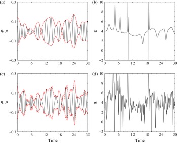
follow from (2.6) while the local frequency follows from (2.7). In order to test the theoretical approach a broad-band spectral example is required, which is provided by the Pierson–Moskowitz spectrum (Pierson & Moskowitz Reference Pierson and Moskowitz1964). The approach works equally well for the JONSWAP spectrum (which is narrower) so that no results for this case are presented. For the Pierson–Moskowitz spectrum on the logarithmic grid an example of results for envelope and local frequency is shown in figure 1. Two cases are shown. The first case is a Pierson–Moskowitz spectrum which is cut off at twice the peak frequency, giving a spectral width
 ${\it\nu}=0.24$
, while the second case has the cut-off at 8 times the peak frequency, which gives
 ${\it\nu}=0.40$
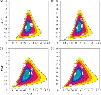
. It is evident that the broad-band spectrum gives a more erratic behaviour in time of the envelope and the local frequency. In addition, note the occasional occurrence of negative local frequencies. Figure 2 shows for the same two cases a comparison of the theoretical joint p.d.f. of envelope wave height and period with the numerical simulation. The agreement is almost perfect, even for the broad-band case. In order to simulate the p.d.f. I have calculated
 ${\it\eta}$
and
 ${\it\zeta}$
for a 500 member ensemble and each time series was 1000 wave periods long. The p.d.f. was determined by counting the number of times the envelope wave height
 $2{\it\rho}$
and local period
 $T$
entered a given wave height and period bin. In the figure wave height is normalized with the significant wave height
 $H_{S}=4m_{0}^{1/2}$
and the local period is normalized with the mean period
 $T01=\overline{{\it\tau}}$
.
Envelope
 ${\it\rho}$
and local frequency
 ${\it\omega}$
for: (a,b) a narrow-band (
 ${\it\nu}=0.24$
) and (c,d) a broad-band (
 ${\it\nu}=0.40$
) signal.

Joint p.d.f. of envelope wave height
 $H/H_{S}$
(with
 $H=2{\it\rho}$
) and period
 $T/T01$
for: (a) a narrow-band (
 ${\it\nu}=0.24$
) and (c) a broad-band (
 ${\it\nu}=0.40$
) case. For comparison the corresponding theoretical distributions are shown in (b) and (d).

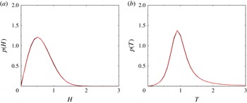
Finally, figure 3 shows, for the broad-band case only, a comparison of the numerically simulated marginal distribution laws with the theoretically ones, given in (2.23) and (2.24). Note that for the period distribution only the positive periods are plotted. For a width
 ${\it\nu}=0.4$
, the fraction of negative periods is only 3.6 % according to theory and only 3.5 % according to the Monte Carlo simulations.
Comparison of simulated (black) and theoretical (red) marginal distribution laws for (a) envelope wave height and (b) period. The spectrum corresponds to the broad-band case (
 ${\it\nu}=0.40$
).

It is concluded that there is good agreement between the theoretical probability distributions and the results obtained with Monte Carlo simulations. This implies that the time series analysis here, which is based on the simple description that
 ${\it\eta}={\it\rho}\cos {\it\phi}$
, where the local frequency follows from the time derivative of the phase, seems to work, even for broad-banded spectra.
4. Extension to weakly nonlinear waves
Having obtained the joint p.d.f. of envelope height and period for linear wave trains we are now going to sketch how to extend the random time series analysis to weakly nonlinear waves. The aim here is to obtain the p.d.f. of the envelope of a weakly nonlinear wave train. Again, we attempt to adopt the simple description
 ${\it\eta}={\it\rho}\cos {\it\phi}$
where envelope
 ${\it\rho}$
and phase
 ${\it\phi}$
are obtained from the surface elevation
 ${\it\eta}$
and its orthogonal complement
 ${\it\zeta}$
which follows from the Hilbert transform of
 ${\it\eta}$
. The orthogonality implies that
 $\langle {\it\eta}{\it\zeta}\rangle$
vanishes. Referring to the development in § 2 the key problem in deriving the envelope p.d.f. is then to obtain a number of statistical parameters. This means, using stationarity of the surface elevation, that we need to obtain in terms of the wave spectrum expressions for the covariances
 $\langle {\it\eta}^{2}\rangle$
and
 $\langle {\it\zeta}^{2}\rangle$
and higher-order cumulants such as skewness and kurtosis and mixed cumulants such as
 $\langle {\it\eta}{\it\zeta}^{2}\rangle$
and
 $\langle {\it\eta}^{2}{\it\zeta}^{2}\rangle$
. For the general case of an arbitrary spectrum a number of these statistical moments have already been derived by Janssen (Reference Janssen2009), which shows that this can be done but, admittedly, the task is quite laborious.
For observed time series it is straightforward to obtain the Hilbert transform of the surface elevation once its Fourier transform is known (see e.g. Shum & Melville Reference Shum and Melville1984). In that event we have for a given time window a representation of
 ${\it\eta}(t)$
in terms of basis functions
 $\exp (-\text{i}{\it\omega}t)$
with fixed Fourier coefficients. Then, as already suggested by Gabor in 1946, the Hilbert transform of the surface elevation follows at once by applying the rule given in (3.6) (see § 3). Note, however, that the spectral values will depend on the length of the time window, and therefore there is an implicit dependence of the results of the Hilbert transform on the stationarity of the signal.
Theoretically, the situation is more complicated because in general the Fourier coefficients will become time-dependent and the Hilbert transform of these coefficients is required as well. However, for weakly nonlinear waves it is possible to obtain an approximate expression for the Hilbert transform of the surface elevation. In that case wave steepness
 ${\it\epsilon}$
is small and it can be shown that the relevant Fourier coefficients only vary on the long time scale
 ${\it\tau}=t/{\it\epsilon}^{2}$
, so that when the Hilbert transform is applied these coefficients can be taken as frozen. The case of weakly nonlinear surface gravity waves is briefly discussed in the appendix A. It is made plausible that since wave–wave interactions only have a relatively small effect on wave evolution, in the weakly nonlinear case it is also possible to find a complex function
 $Z$
, which vanishes for
 $\text{Im}(t)\rightarrow -\infty$
, in such a way that
 ${\it\eta}=(Z+Z^{\ast })/2$
while
 ${\it\zeta}=-\text{i}(Z-Z^{\ast })/2$
.
In order now to obtain the envelope wave height distribution the joint p.d.f. of the two orthogonal quantities
 ${\it\eta}$
and
 ${\it\zeta}$
is required. The joint p.d.f. follows from the so-called generating or characteristic function. Here, the characteristic function for
 $N$
parameters
 $\boldsymbol{x}=(x_{1},x_{2},\dots ,x_{N})$
is defined by
 $$\begin{eqnarray}G({\bf\mu})=\langle \exp \text{i}{\bf\mu}\boldsymbol{\cdot }\boldsymbol{x}\rangle =\int \text{d}\boldsymbol{x}\;p(\boldsymbol{x})\exp \text{i}{\bf\mu}\boldsymbol{\cdot }\boldsymbol{x},\end{eqnarray}$$
and the parameter
 ${\bf\mu}$
represents the counterpart of
 $\boldsymbol{x}$
in Fourier space. Clearly, the joint p.d.f.
 $p(\boldsymbol{x})$
is the Fourier transform of the generating function
 $G$
. Now, for weakly nonlinear waves an expansion of
 $p(\boldsymbol{x})$
in terms of statistical moments is obtained by expanding
 $G$
and then
 $p(\boldsymbol{x})$
follows from the Fourier transform of
 $G$
.
Note that
 $G$
contains all the statistical information on the stochastic process
 $\boldsymbol{x}$
, e.g. the moments of the p.d.f. are related to derivatives of
 $G$
with respect to
 ${\bf\mu}$
at the origin. Hence, the moments are related to the coefficients of the Taylor expansion around the origin. This expansion is, however, not very useful because it does not bring out the significance of a special characteristic distribution, the one corresponding to a Gaussian distribution, which is of great importance as linear waves usually have a normal distribution. Here the Gaussian characteristic function is given by
 $$\begin{eqnarray}G_{0}=\text{e}^{-{\it\mu}_{i}{\it\mu}_{j}B_{ij}/2},\end{eqnarray}$$
and by expanding
 $G$
around
 $G_{0}$
the so-called cumulants of the distribution function are introduced. These are the coefficients of the Taylor expansion of the logarithm of
 $G$
, i.e.
 $$\begin{eqnarray}G=\exp \left\{-\frac{1}{2}{\it\mu}_{i}{\it\mu}_{j}B_{ij}-\frac{\text{i}}{3!}{\it\mu}_{i}{\it\mu}_{j}{\it\mu}_{k}C_{ijk}+\frac{1}{4!}{\it\mu}_{i}{\it\mu}_{j}{\it\mu}_{k}{\it\mu}_{l}D_{ijkl}+\cdots \!\right\},\end{eqnarray}$$
where
 $B_{ij}$
is the second-order cumulant,
 $C_{ijk}$
is the third-order cumulant, related to the skewness and, finally,
 $D_{ijkl}$
is the fourth-order cumulant which is connected to the excess kurtosis. Consistent with the small-amplitude expansion for waves with a small steepness
 ${\it\epsilon}$
, there is an ordering in the magnitude of the cumulants, i.e.
 $$\begin{eqnarray}B_{ij}=\mathit{O}({\it\epsilon}^{2}),\quad C_{ijk}=\mathit{O}({\it\epsilon}^{4}),\quad D_{ijkl}=\mathit{ O}({\it\epsilon}^{6}),\end{eqnarray}$$
and the hope is that for sufficiently small
 ${\it\epsilon}$
the expansion converges. In order to obtain the joint p.d.f. the Fourier transform of
 $G$
is required, which for the expansion given in (4.3) is not straightforward. Therefore the exponential function is expanded. Adopting the above ordering one finds to lowest significant order
 $$\begin{eqnarray}G\simeq G_{0}\left\{1-\frac{\text{i}}{3!}{\it\mu}_{i}{\it\mu}_{j}{\it\mu}_{k}C_{ijk}+\frac{1}{4!}{\it\mu}_{i}{\it\mu}_{j}{\it\mu}_{k}{\it\mu}_{l}D_{ijkl}-\frac{1}{72}\left({\it\mu}_{i}{\it\mu}_{j}{\it\mu}_{k}C_{ijk}\right)^{2}\!\right\}.\end{eqnarray}$$
The corresponding expansion for the p.d.f.
 $p(\boldsymbol{x})$
then follows from the Fourier transform of
 $G$
, i.e.
 $$\begin{eqnarray}p(\boldsymbol{x})=\frac{1}{(2{\rm\pi})^{N}}\int \text{d}{\bf\mu}G({\bf\mu})\exp (-\text{i}{\bf\mu}\boldsymbol{\cdot }\boldsymbol{x}).\end{eqnarray}$$
Noting the usual rule for Fourier transformation, namely that each factor
 ${\it\mu}_{i}$
corresponds to
 $\text{i}\partial /\partial x_{i}$
and denoting the Fourier transform of
 $G_{0}$
by
 ${\it\Phi}_{0}$
where
 $$\begin{eqnarray}{\it\Phi}_{0}=\frac{1}{(2{\rm\pi})^{N/2}|B|^{1/2}}\exp \left(-\frac{1}{2}x_{i}x_{j}B_{ij}^{-1}\right),\end{eqnarray}$$
the expansion for the p.d.f.
 $p(\boldsymbol{x})$
becomes
 $$\begin{eqnarray}p(\boldsymbol{x})=\left\{1-\frac{C_{ijk}}{3!}\frac{\partial ^{3}}{\partial x_{i}\partial x_{j}\partial x_{k}}+\frac{D_{ijkl}}{4!}\frac{\partial ^{4}}{\partial x_{i}\partial x_{j}\partial x_{k}\partial x_{l}}+\frac{C_{ijk}^{2}}{72}\left(\frac{\partial ^{3}}{\partial x_{i}\partial x_{j}\partial x_{k}}\right)^{2}\!\right\}{\it\Phi}_{0}(\boldsymbol{x})\end{eqnarray}$$
which is known as the Edgeworth expansion. Compared to the well-known Gram–Charlier expansion, used by e.g. Tayfun & Lo (Reference Tayfun and Lo1990), the difference is the additional term which is proportional to the square of the skewness parameter
 $C_{ijk}$
. According to the order of magnitude of skewness and kurtosis, given in (4.4), the last term of the Edgeworth expansion is, at least in the tail of the distribution on the scale
 $x_{i}=O(1/{\it\epsilon})$
, as important as the term involving the kurtosis
 $D_{ijkl}$
. Therefore, it should be retained and it gives an important contribution to the tail of the wave height distribution as will be seen in a moment.
Equation (4.8) has been applied to the case of the joint p.d.f. of
 ${\it\eta}$
and
 ${\it\zeta}$
. Polar coordinates
 ${\it\rho}$
and
 ${\it\theta}$
are introduced, i.e.
 $$\begin{eqnarray}{\it\eta}={\it\rho}\cos {\it\theta},\quad {\it\zeta}={\it\rho}\sin {\it\theta},\end{eqnarray}$$
and following the approach given in Mori & Janssen (Reference Mori and Janssen2006) the p.d.f. of the envelope
 ${\it\rho}$
is then obtained from an integration of the joint p.d.f. over
 ${\it\theta}$
from 0 to
 $2{\rm\pi}$
. For convenience it will be assumed that the variances of
 ${\it\eta}$
and
 ${\it\zeta}$
are equal and that these parameters are orthogonal in the sense that
 $\langle {\it\eta}{\it\zeta}\rangle =0$
. Results will be presented for the scaled parameters
 ${\it\eta}^{\prime }={\it\eta}/\langle {\it\eta}^{2}\rangle ^{1/2}$
and
 ${\it\zeta}^{\prime }={\it\eta}/\langle {\it\zeta}^{2}\rangle ^{1/2}$
and the primes will be dropped. Because of this normalization, the parameters that measure the deviation from normality, namely skewness and kurtosis, are scaled accordingly. Introducing the normalized moments
 $$\begin{eqnarray}\displaystyle {\it\lambda}_{m,n}=\frac{\langle {\it\eta}^{m}{\it\zeta}^{n}\rangle }{\langle {\it\eta}^{2}\rangle ^{m/2}\langle {\it\zeta}^{2}\rangle ^{n/2}},\end{eqnarray}$$
the normalized skewness becomes
 $$\begin{eqnarray}{\it\kappa}_{m,n}={\it\lambda}_{m,n},\quad m+n=3,\end{eqnarray}$$
while the normalized kurtosis becomes
 $$\begin{eqnarray}{\it\kappa}_{m,n}={\it\lambda}_{m,n}+(m-1)(n-1)(-1)^{m/2},\quad m+n=4.\end{eqnarray}$$
As a result, the envelope p.d.f. becomes
 $$\begin{eqnarray}p({\it\rho})={\it\rho}\text{e}^{-{\it\rho}^{2}/2}\left\{1+\frac{{\it\kappa}_{4}}{8}\left(\frac{1}{8}{\it\rho}^{4}-{\it\rho}^{2}+1\right)+\frac{{\it\kappa}_{3}^{2}}{72}\left(\frac{1}{16}{\it\rho}^{6}-\frac{9}{8}{\it\rho}^{4}+\frac{9}{2}{\it\rho}^{2}-3\right)\!\right\},\end{eqnarray}$$
with
 $$\begin{eqnarray}{\it\kappa}_{3}^{2}=5(k_{30}^{2}+{\it\kappa}_{03}^{2})+9({\it\kappa}_{21}^{2}+{\it\kappa}_{12}^{2})+6({\it\kappa}_{30}{\it\kappa}_{12}+{\it\kappa}_{03}{\it\kappa}_{21})\end{eqnarray}$$
and
 $$\begin{eqnarray}{\it\kappa}_{4}={\it\kappa}_{40}+{\it\kappa}_{04}+2{\it\kappa}_{22}.\end{eqnarray}$$
The envelope p.d.f. consists of three contributions. The first term is the dominant one and represents the usual Rayleigh distribution also found in § 2. The other two terms, proportional to kurtosis and skewness, represent deviations from normality and are supposed to be small corrections to the Rayleigh distribution. However, from (4.13) it is immediately evident that for large
 ${\it\rho}$
the nonlinear terms will dominate. Thus, the expansion is not uniformly valid and has a limited range of validity. This is also evident when the theoretical result is compared with Monte Carlo simulations.
It is noted that Mori & Janssen (Reference Mori and Janssen2006) used as starting point the Gram–Charlier expansion for the joint p.d.f. of
 ${\it\eta}$
and
 ${\it\zeta}$
. The reason for this was that they mainly concentrated on the contribution of free waves to the deviations from normality. For free waves the skewness of the sea surface can be shown to vanish (see appendix A) and therefore the third term in (4.13) was ignored. Here, it is shown that for bound waves the third term should be included.
In order to agree with the common practice of using the wave height distribution for the study of extreme sea states a change of variable from envelope height normalized with the variance
 $\langle {\it\eta}^{2}\rangle ^{1/2}$
of the time series to wave height normalized with the significant wave height
 $H_{S}=4\langle {\it\eta}^{2}\rangle ^{1/2}$
is introduced, where local wave height is given by twice the envelope height. Denoting the normalized wave height by
 $h$
one then finds that
 $h={\it\rho}/2$
and from (4.13) the p.d.f. of
 $h$
becomes
 $$\begin{eqnarray}p(h)=4h\text{e}^{-2h^{2}}\left\{1+\frac{{\it\kappa}_{4}}{3}\left(2h^{4}-4h^{2}+1\right)+\frac{{\it\kappa}_{3}^{2}}{72}\left(4h^{6}-18h^{4}+18h^{2}-3\right)\!\right\}.\end{eqnarray}$$
In principle, it is straightforward to evaluate for an arbitrary sea state all the coefficients in (4.16). To be specific,
 ${\it\kappa}_{40}$
and
 ${\it\kappa}_{30}$
are already known from Janssen (Reference Janssen2009), but
 ${\it\kappa}_{22}$
and
 ${\it\kappa}_{04}$
still need to be determined. Clearly this is a rather cumbersome task; therefore, to validate the present approach only the case of a single wave train will be considered, which may be regarded as the narrow-band limit of a weakly nonlinear, random sea state. In that case the surface elevation is given by the well-known Stokes expansion (see appendix A for more details)
 $$\begin{eqnarray}{\it\eta}/a=\left(1-\frac{{\it\epsilon}^{2}}{8}\right)\cos {\it\theta}+\frac{1}{2}{\it\epsilon}\cos 2{\it\theta}+\frac{3}{8}{\it\epsilon}^{2}\cos 3{\it\theta},\end{eqnarray}$$
where
 $a$
is the wave amplitude,
 ${\it\epsilon}=k_{0}a$
is the wave slope,
 ${\it\theta}=k_{0}x-{\it\Omega}_{0}t+{\it\phi}$
,
 ${\it\phi}$
is the arbitrary, random phase of the wave and
 ${\it\Omega}_{0}={\it\omega}_{0}(1+{\it\epsilon}^{2}/2)$
is the nonlinear dispersion relation with
 ${\it\omega}_{0}=\sqrt{gk_{0}}$
. The auxiliary variable
 ${\it\zeta}$
is then obtained by replacing all cosines with sines times a ‘minus’ sign.
In order to evaluate the p.d.f. of the wave height the evaluation of a number of skewness and kurtosis terms is required. To that end the method used in Janssen (Reference Janssen2009) (cf. § A.3 therein) is followed which means that it is assumed that the wave amplitude
 $a$
has a Rayleigh distribution while the phase
 ${\it\phi}$
is uniform. With
 ${\it\sigma}^{2}=\langle a^{2}\rangle$
the wave variance and
 ${\rm\Delta}=k_{0}{\it\sigma}$
the so-called significant slope parameter, it is then found that the relevant skewness terms become
 $$\begin{eqnarray}{\it\kappa}_{30}=3{\rm\Delta},\quad {\it\kappa}_{12}={\rm\Delta},\quad {\it\kappa}_{21}={\it\kappa}_{03}=0,\end{eqnarray}$$
while the relevant kurtosis terms become
 $$\begin{eqnarray}{\it\kappa}_{40}=18{\rm\Delta}^{2},\quad {\it\kappa}_{22}=3{\rm\Delta}^{2},\quad {\it\kappa}_{04}=0.\end{eqnarray}$$
It is striking to see that the statistical parameters for
 ${\it\eta}$
and
 ${\it\zeta}$
are so different. Whilst
 ${\it\eta}$
is a nonlinear signal with finite skewness and kurtosis, its Hilbert transform
 ${\it\zeta}$
is also a nonlinear signal but with vanishing third and fourth cumulant. Using (4.18) and (4.19) in (4.16) the wave height p.d.f. of a third-order Stokes wave train becomes
 $$\begin{eqnarray}p(h)=4h\text{e}^{-2h^{2}}\left\{\!1+4{\rm\Delta}^{2}\left({\textstyle \frac{3}{2}}h^{2}-3h^{4}+h^{6}\right)\!\right\}.\end{eqnarray}$$
Finally, in order to check the validity of the theoretical result (4.20) Monte Carlo simulations using the surface elevation (4.17), with Rayleigh distributed amplitude
 $a$
and uniform phase
 ${\it\phi}$
, and its corresponding Hilbert transform were performed. The envelope then follows from (2.6), and the wave height distribution follows at once. In order to obtain statistically reliable results, in particular in the tail of the distribution, the number of ensemble members was 5 000 000.
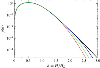
In figure 4 a comparison is made between (4.20) and the result of the Monte Carlo simulation. The significant steepness
 ${\rm\Delta}$
was chosen to be 0.1 which is a typically value for steep, young windsea. Concentrating on the tail of the distribution the logarithm of the p.d.f. versus normalized wave height has been plotted, hence a Gaussian distribution appears as a parabola while an exponential distribution is a straight line. It is striking to see that the Monte Carlo simulations show, to high precision, that the tail of the distribution is exponential. It has already been noted that the theoretical result, given by the blue line in figure 4, is not uniformly valid. Hence theory can at best only agree in a limited range of
 $h$
with the Monte Carlo results. Figure 4 suggests that there is good agreement up to
 $h\simeq 2.5$
, but it is emphasized that the range of validity depends on the wave steepness, i.e. for steeper waves the range is smaller.
Comparison of simulated (black) and theoretical (blue) probability distribution laws for local wave height normalized with its mean value (the significant wave height). The signal is given by a Stokes wave train with significant steepness of 0.1. For illustration the wave height distribution for a Gaussian sea state is shown by the red line, while the theoretical p.d.f. without skewness effects is shown by the green line.

Furthermore, by comparing the p.d.f. for a Gaussian sea state (red line) with the Monte Carlo result it is evident that for young windsea even the contributions by the bound waves may result in considerable deviations from the normal distribution, leading to considerable increases in the probability of extreme events. For example, the probability that wave height is larger than two times significant wave height increases by almost a factor of three, from
 $3.6\times 10^{-4}$
to
 $9.8\times 10^{-4}$
. Finally, by comparing the green curve with the blue one it is seen that finite skewness has a considerable impact on the tail of the distribution. It is emphasized that this result holds for the bound wave contribution to the statistics of a weakly nonlinear, random sea state. The free waves statistics is different because skewness can be shown to be vanishingly small. Therefore, as already shown by Mori & Janssen (Reference Mori and Janssen2006), for free waves the wave height distribution is given by (4.16) with vanishing skewness contribution, i.e.
 ${\it\kappa}_{3}^{2}=0$
.
5. Conclusions
In this paper an analysis method has been studied that allows the characterization of extreme events in a random time series. The idea is to obtain the joint p.d.f. of envelope wave height and period from the envelope
 ${\it\rho}$
and the local phase
 ${\it\phi}$
of the wave train, and wave height is then defined as twice the envelope height while the local period follows from the angular frequency given by
 ${\it\omega}=-\partial {\it\phi}/\partial t$
. Envelope and phase are obtained from the time series of the signal
 ${\it\eta}$
and its Hilbert transform. The envelope has the interesting physical interpretation that its square is a measure of the power of the signal. The physical interpretation of the local period is not always clear as there is no guarantee that this quantity is always positive, and the frequency with which negative periods occur, although small, increases with the width of the wave spectrum.
Nevertheless, it turns out that the reduction of a complicated signal to just two parameters provides useful information on the statistical properties of the time series. For example, for a Gaussian sea state it is straightforward to obtain the joint p.d.f. of envelope wave height and wave period. A comparison with Monte Carlo simulations suggests that this conclusion not only holds for narrow-band wave trains, but also for time series with a fairly arbitrary spectral shape, the only restriction being that a number of spectral moments should exist. For the joint p.d.f. of wave height and period marginal distribution laws can be derived as well, and the p.d.f. of envelope wave height is shown to follow, independent of spectral width, the Rayleigh distribution.
It has also been shown how the present approach can be extended into the weakly nonlinear regime. This is, of course, quite relevant when one wishes to study extreme events such as freak waves because nonlinear effects are expected to be important. In the present work the starting point to study nonlinear effects on the p.d.f. was the well-known Edgeworth expansion. Unfortunately, this expansion is not uniformly valid, but for typical values of skewness and kurtosis seems to give acceptable estimates of the probability of extreme events for
 $h<2.5$
, where
 $h$
is the envelope wave height normalized with the significant wave height. Monte Carlo simulations seem to indicate that the tail of the distribution is exponential, which is beyond the grasp of the Edgeworth expansion. More work is therefore needed to extend the weakly nonlinear statistical approach to allow for the exponential behaviour of the tail of the p.d.f.
Acknowledgements
Useful discussions with S. Abdalla are much appreciated. The author thanks A. Janssen and V. Shrira, who both suggested publishing this work.
Appendix A. Hilbert transform for surface elevation of weakly nonlinear waves
Assuming potential flow of an ideal fluid with potential
 ${\it\phi}$
, Zakharov (Reference Zakharov1968) has shown that the total energy
 $E$
of the fluid may be used as a Hamiltonian when one chooses as canonical variables the surface elevation
 ${\it\eta}$
and the value
 ${\it\psi}$
of the potential at the surface, i.e.
 ${\it\psi}(\boldsymbol{x},t)={\it\phi}(\boldsymbol{x},z,t)$
. Here, coordinates are chosen in such a way that the undisturbed surface of the fluid coincides with the
 $x{-}y$
plane, while the
 $z$
-axis is pointed upward and the acceleration due to gravity
 $g$
is pointed downward.
For weakly nonlinear waves Zakharov (Reference Zakharov1968) obtained from the Hamilton equations an approximate evolution equation for surface gravity waves which in essence describes the evolution of the amplitude of the waves caused by four-wave interactions. In this approach the surface elevation and potential at the surface are written in terms of a Fourier expansion. Introducing
 $\boldsymbol{k}$
as the wavenumber vector,
 $k$
as its magnitude, while
 ${\it\omega}={\it\omega}(k,D)$
denotes the dispersion relation of surface gravity waves on water of finite depth
 $D$
, the canonical variables
 ${\it\eta}$
and
 ${\it\psi}$
become
 $$\begin{eqnarray}{\it\eta}=\int _{-\infty }^{\infty }\text{d}\boldsymbol{k}\;\hat{{\it\eta}}(\boldsymbol{k},t)\text{e}^{\text{i}\boldsymbol{k}\boldsymbol{\cdot }\boldsymbol{x}}+\text{c.c.},\quad {\it\psi}=\int _{-\infty }^{\infty }\text{d}\boldsymbol{k}\;\hat{{\it\psi}}(\boldsymbol{k},t)\text{e}^{\text{i}\boldsymbol{k}\boldsymbol{\cdot }\boldsymbol{x}}+\text{c.c.},\end{eqnarray}$$
where
 $\hat{{\it\eta}}(\boldsymbol{k},t)=\sqrt{({\it\omega}/2g)}B(\boldsymbol{k},t)$
,
 $\hat{{\it\psi}}(\boldsymbol{k},t)=-\text{i}\sqrt{(g/2{\it\omega})}B(\boldsymbol{k},t)$
and
 $B(\boldsymbol{k},t)$
is the action variable. It is remarked that the variable
 $\hat{{\it\eta}}$
and
 $\hat{{\it\psi}}$
are in quadrature: they are out of phase by 90°.
The Fourier expansions for
 ${\it\eta}$
and
 ${\it\psi}$
are then substituted into the expression for the energy
 $E$
, and assuming small steepness
 ${\it\epsilon}$
an expansion of
 $E$
in powers of the action variable
 $B$
is obtained. Then, the evolution equation for
 $B$
follows from Hamilton’s equations
 $\partial B/\partial t=-\text{i}{\it\delta}E/{\it\delta}B^{\ast }$
, and it turns out that the rate of change in time of
 $B$
is caused by three terms. The first one, which is linear in
 $B$
, is the dominant term and results in a harmonic oscillation with angular frequency
 ${\it\omega}$
. The second and third terms are nonlinear in the action variable and they describe the rate of change in time caused by three-wave and four-wave interactions, respectively. Surface gravity waves, because the dispersion relation is concave, do not have resonant three-wave interactions, while Phillips (Reference Phillips1960) has shown that only one type of resonant four-wave interaction is permitted by the dispersion relation, namely interactions that satisfy the condition
 ${\it\omega}_{1}+{\it\omega}_{2}={\it\omega}_{3}+{\it\omega}_{4}$
for
 $\boldsymbol{k}_{1}+\boldsymbol{k}_{2}=\boldsymbol{k}_{3}+\boldsymbol{k}_{4}$
. The distinction between resonant and non-resonant interactions has important consequences, namely, non-resonant interactions, which give rise to bound harmonics, may be eliminated by means of a canonical transformation that is non-singular (Zakharov Reference Zakharov1968; Krasitskii Reference Krasitskii1994).
In order to eliminate as much as possible the effects of the bound waves, one therefore applies on
 $B$
a canonical transformation of the type
 $$\begin{eqnarray}B=b+B_{2}(b,b^{\ast }),\end{eqnarray}$$
where
 $b$
is the action variable of the free gravity waves while
 $B_{2}(b,b^{\ast })$
is a representation of the bound waves. The transformation
 $B_{2}(b,b^{\ast })$
is only known in terms of an amplitude expansion, and an expression up to third order is required (Krasitskii Reference Krasitskii1994; Janssen Reference Janssen2009). As an illustration the expression up to second order in steepness is given:
 $$\begin{eqnarray}B_{2}=\int \text{d}\boldsymbol{k}_{2,3}\left\{A_{1,2,3}^{(1)}b_{2}b_{3}{\it\delta}_{1-2-3}+A_{1,2,3}^{(2)}b_{2}^{\ast }b_{3}{\it\delta}_{1+2-3}+A_{1,2,3}^{(3)}b_{2}^{\ast }b_{3}^{\ast }{\it\delta}_{1+2+3}\!\right\}+\cdots\end{eqnarray}$$
where, for brevity, the notation
 $b_{1}=b(\boldsymbol{k}_{1})$
, etc., is introduced. The unknowns
 $A^{(i)},$
 $i=1,3$
are obtained by systematically removing the non-resonant third-order contributions to the wave energy.
As a consequence, the evolution equation for
 $b$
becomes
 $$\begin{eqnarray}\frac{\partial b_{1}}{\partial t}+\text{i}{\it\omega}_{1}b_{1}=-\text{i}\int \text{d}\boldsymbol{k}_{2,3,4}T_{1,2,3,4}b_{2}^{\ast }b_{3}b_{4}{\it\delta}_{1+2-3-4},\end{eqnarray}$$
which is called the Zakharov equation. It describes the rate of change of the free wave action variable
 $b$
due to one particular type of nonlinear interaction only, namely
 $\boldsymbol{k}_{1}+\boldsymbol{k}_{2}=\boldsymbol{k}_{3}+\boldsymbol{k}_{4}$
. The nonlinear transfer function
 $T_{1,2,3,4}$
, as found by Krasitskii (Reference Krasitskii1994), enjoys a number of symmetries that guarantee that the Zakharov equation is Hamiltonian and conserves energy.
In Janssen (Reference Janssen2003) it was shown that according to the deep-water version of the Zakharov equation extreme wave events are generated by nonlinear focusing in a random wavefield, resulting in considerable enhancement of the probability of extreme waves (which basically prompted the present study). Therefore, the nonlinear focusing gives rise to deviations from the normal probability distribution and is strongly connected to the dynamics of the free waves. However, it is also of interest to study the consequences of the presence of bound waves on the surface elevation statistics (see for an extensive study Janssen Reference Janssen2009). Bound waves will give rise to sharper crests and wider troughs which will result in deviations from the normal distribution as well. Based on the canonical transformation (A 2) the surface elevation is therefore written as a sum of the free wave contribution
 ${\it\eta}_{free}$
and a contribution from the bound waves
 ${\it\eta}_{bound}$
, i.e.
 $$\begin{eqnarray}{\it\eta}={\it\eta}_{free}+{\it\eta}_{bound},\end{eqnarray}$$
where
 ${\it\eta}_{free}$
is given by (A 1) with
 $\hat{{\it\eta}}_{free}(\boldsymbol{k},t)=({\it\omega}/2g)^{1/2}b(\boldsymbol{k},t)$
while
 ${\it\eta}_{bound}$
is given by (A 1) but now using, in agreement with the canonical transformation (A 2), the contribution of the bound waves, i.e.
 $\hat{{\it\eta}}_{bound}(\boldsymbol{k},t)=({\it\omega}/2g)^{1/2}B_{2}(\boldsymbol{k},t)$
.
Now, we are in a position to derive an approximate expression for the Hilbert transform of the surface elevation. In doing so it is assumed that to a good approximation the dynamics of the free wave action variable
 $b(\boldsymbol{k})$
is given by a harmonic oscillator with angular frequency
 ${\it\omega}(k)$
. In other words in (A 4) effects of nonlinear interactions are ignored, and in the evaluation of the Hilbert transform we take the simple linear solution
 $$\begin{eqnarray}b(\boldsymbol{k},t)=\hat{b}(\boldsymbol{k},{\it\tau})\;\text{e}^{-\text{i}{\it\omega}(k)t}\end{eqnarray}$$
and from the Zakharov equation it follows that
 $\hat{b}$
evolves on the slow time scale
 ${\it\tau}={\it\epsilon}^{2}t$
.
A.1. Free waves
Let us first start with the free wave part of the surface elevation. Inspection of the expression for the surface elevation suggests introducing the following complex function:
 $$\begin{eqnarray}Z_{free}=2\int _{-\infty }^{\infty }\text{d}\boldsymbol{k}\;\hat{{\it\eta}}_{free}(\boldsymbol{k})\text{e}^{\text{i}\boldsymbol{k}\boldsymbol{\cdot }\boldsymbol{x}},\end{eqnarray}$$
so that in agreement with (4.1) the surface elevation becomes
 $$\begin{eqnarray}{\it\eta}={\textstyle \frac{1}{2}}\left(Z_{free}+Z_{free}^{\ast }\right).\end{eqnarray}$$
Writing the time evolution in the form given in (A 6) and ignoring the slow time dependence, it is seen that just as in § 2 the complex function
 $Z$
vanishes for
 $\text{Im}(t)\rightarrow -\infty$
, hence the auxiliary variable becomes
 ${\it\zeta}=-H({\it\eta})$
. Assuming that the amplitudes vary on a slow time scale while using (3.6) one finds that
 $H({\it\eta})\approx (\text{i}/2)(Z-Z^{\ast })$
, therefore, the appropriate auxiliary variable becomes
 $$\begin{eqnarray}{\it\zeta}=-\frac{\text{i}}{2}(Z_{free}-Z_{free}^{\ast }).\end{eqnarray}$$
It is remarkable that the pair
 $({\it\eta},{\it\zeta})$
enjoys a similar relation to the canonical variables
 ${\it\eta}$
and
 ${\it\psi}$
of the Hamiltonian formulation of water waves, i.e.
 ${\it\zeta}$
is 90° out of phase with
 ${\it\eta}$
. The envelope
 ${\it\rho}$
and phase
 ${\it\phi}$
are introduced according to
 $Z={\it\rho}\text{e}^{\text{i}{\it\phi}}$
, hence
 $$\begin{eqnarray}{\it\eta}={\it\rho}\cos {\it\phi},\quad {\it\zeta}={\it\rho}\sin {\it\phi};\end{eqnarray}$$
therefore envelope and phase may be obtained in the usual manner. Although we only have an approximate expression for
 ${\it\zeta}$
it is worthwhile to point out that for homogeneous and stationary conditions it still follows that surface elevation and auxiliary variable are orthogonal, i.e.
 $\langle {\it\eta}{\it\zeta}\rangle =0$
. For homogeneous water waves the spatial correlation function only depends on the distance between the two locations of interest. As a consequence this implies for the second moments
 $$\begin{eqnarray}\langle b_{1}b_{2}^{\ast }\rangle =N_{1}{\it\delta}(\boldsymbol{k}_{1}-\boldsymbol{k}_{2})\quad \text{and}\quad \langle b_{1}b_{2}\rangle =0,\end{eqnarray}$$
where we have introduced the usual action density
 $N(\boldsymbol{k})$
. Using (A 8) and (A 9) the correlation between
 ${\it\eta}$
and
 ${\it\zeta}$
becomes
 $$\begin{eqnarray}\langle {\it\eta}{\it\zeta}\rangle ={\textstyle \frac{1}{4}}\left(\langle Z_{free}^{2}\rangle -\langle (Z_{free}^{\ast })^{2}\rangle \right)=0,\end{eqnarray}$$
and because of the second homogeneity condition in (A 11) both the first and the second term on the right-hand side vanish. For the same reason one can show that the second moments of
 ${\it\eta}$
and
 ${\it\zeta}$
are identical, i.e.
 $m_{0}=\langle {\it\eta}^{2}\rangle =\langle {\it\zeta}^{2}\rangle$
, where
 $m_{0}$
is the zeroth moment of the spectrum.
As indicated in Mori & Janssen (Reference Mori and Janssen2006), who originally introduced the auxiliary parameter
 ${\it\zeta}$
of (A 9), higher-order moments/cumulants can be obtained as well. Using the properties of the Zakharov equation, which has cubic nonlinearity, and the homogeneity assumption it can be shown that to lowest significant order the free waves do not contribute to the skewness of the sea surface, i.e.
 $\langle {\it\eta}^{3}\rangle =0$
,
 $\langle {\it\eta}^{2}{\it\zeta}\rangle =0$
,
 $\langle {\it\eta}{\it\zeta}^{2}\rangle =0$
and
 $\langle {\it\zeta}^{3}\rangle =0$
. As will be seen in the next subsection the skewness of the sea surface is entirely determined by the bound waves.
However, as pointed out by Janssen (Reference Janssen2003) free waves will contribute to the kurtosis of the sea surface, because of the action of the resonant and non-resonant four-wave interactions. The excess kurtosis
 ${\it\kappa}_{40}=\langle {\it\eta}^{4}\rangle /m_{0}^{2}-3$
is given by (14) of Mori & Janssen (Reference Mori and Janssen2006), and for a narrow-band, uni-directional wave train the kurtosis can be shown to depend on the square of the Benjamin–Feir Index. Other fourth-order cumulants that are needed for the evaluation of the p.d.f. of the envelope wave height are
 ${\it\kappa}_{22}=\langle {\it\eta}^{2}{\it\zeta}^{2}\rangle /m_{0}^{2}-1$
and
 ${\it\kappa}_{04}=\langle {\it\zeta}^{4}\rangle /m_{0}^{2}-3$
. Using the pair (A 8) and (A 9) and the homogeneity condition one finds
 ${\it\kappa}_{22}={\it\kappa}_{40}/3$
, while
 ${\it\kappa}_{04}={\it\kappa}_{40}$
.
The p.d.f. of envelope wave height and the resulting p.d.f. of maximum wave height can then be obtained following the procedure sketched in Mori & Janssen (Reference Mori and Janssen2006). The paper treats the nonlinear free waves, which give the dominant contribution to changes in the p.d.f. in the case of extreme events such as freak waves. However, bound waves need to be treated somewhat differently as will be seen in the next subsection.
A.2. Bound waves
The case of bound waves is not as straightforward as the free wave case. In the previous subsection we have seen that it is trivial to obtain the appropriate complex function
 $Z_{free}$
(see (A 9)) because, at least to second order in steepness, all modes behave like
 $\exp (-\text{i}{\it\omega}t)$
and therefore they decay in time for
 $\text{Im}(t)\rightarrow -\infty$
. Then, under the assumption of frozen amplitude, the Hilbert transform of
 $Z_{free}$
follows at once.
The nonlinear part of the canonical transformation is given in (A 2) and from the expression below (A 3) it is evident that there is a mixed large-time behaviour. The term proportional to
 $b_{2}b_{3}$
oscillates like
 $\exp (-\text{i}({\it\omega}_{2}+{\it\omega}_{3})t)$
hence it vanishes for
 $\text{Im}(t)\rightarrow -\infty$
. On the other hand, the term proportional to
 $b_{2}^{\ast }b_{3}^{\ast }$
oscillates like
 $\exp (+\text{i}({\it\omega}_{2}+{\it\omega}_{3})t)$
so it will vanish for positive imaginary time, while the behaviour of the mixed term
 $b_{2}^{\ast }b_{3}$
depends on the sign of
 ${\it\omega}_{2}-{\it\omega}_{3}$
. However, in the expression for the bound part of the surface elevation terms with similar time-asymptotic behaviour can be grouped together suggesting the following complex function for the bound waves:
 $$\begin{eqnarray}Z_{bound}=2\int _{-\infty }^{\infty }\text{d}\boldsymbol{k}_{1}\;\hat{{\it\eta}}_{bound}\;\exp (\text{i}\boldsymbol{k}_{1}\boldsymbol{\cdot }\boldsymbol{x})\end{eqnarray}$$
where
 $$\begin{eqnarray}\displaystyle \hat{{\it\eta}}_{bound} & = & \displaystyle \left(\frac{{\it\omega}_{1}}{2g}\right)^{1/2}\int _{-\infty }^{\infty }\text{d}\boldsymbol{k}_{2,3}\left\{\!\left(A_{1,2,3}^{(1)}+A_{-1,2,3}^{(3)}\right)b_{2}b_{3}{\it\delta}_{1-2-3}\right.\nonumber\\ \displaystyle & & \displaystyle +\left.\left(A_{1,2,3}^{(2)}+A_{-1,2,3}^{(2)}\right)b_{2}^{\ast }b_{3}H({\it\omega}_{3}-{\it\omega}_{2}){\it\delta}_{1+2-3}\right\}+\cdots \,,\end{eqnarray}$$
where
 $H$
is the Heaviside function and the dots represent the third-order terms that determine the kurtosis related to the bound waves. With this definition of the complex function one may proceed as before and one obtains the pair of functions
 $$\begin{eqnarray}{\it\eta}=\frac{1}{2}\left(Z_{bound}+Z_{bound}^{\ast }\right),\quad {\it\zeta}=-\frac{\text{i}}{2}\left(Z_{bound}-Z_{bound}^{\ast }\right).\end{eqnarray}$$
In principle it is now straightforward, but very laborious, to obtain the relevant cumulants which are needed to obtain the p.d.f. of envelope wave height (Janssen Reference Janssen2009). Rather than studying the general case we will consider instead the simple case of a uniform nonlinear Stokes wave. Up to third order in wave steepness the canonical transformation for a single deep-water wave train is found to be
 $$\begin{eqnarray}{\it\eta}/a=\left(1-\frac{{\it\epsilon}^{2}}{8}\right)\cos {\it\theta}+\frac{1}{2}{\it\epsilon}\cos 2{\it\theta}+\frac{3}{8}{\it\epsilon}^{2}\cos 3{\it\theta},\end{eqnarray}$$
where
 $a$
is the wave amplitude,
 ${\it\epsilon}=k_{0}a$
is the wave slope,
 ${\it\theta}=k_{0}x-{\it\Omega}_{0}t+{\it\phi}$
,
 ${\it\phi}$
is the arbitrary phase of the wave and
 ${\it\Omega}_{0}={\it\omega}_{0}(1+{\it\epsilon}^{2}/2)$
is the nonlinear dispersion relation with
 ${\it\omega}_{0}=\sqrt{gk_{0}}$
. The above single-mode result follows from the narrow-band limit of the canonical transformation for general wave spectra (Janssen Reference Janssen2009). The auxiliary variable
 ${\it\zeta}$
is then obtained by taking the Hilbert transform of the surface elevation. For the expression (A 16) this is a straightforward task as it simply means that the cosines are replaced by sines times a ‘minus’ sign. Alternatively, one may obtain
 ${\it\zeta}$
using (A 15) by inferring from (A 16) that
 $$\begin{eqnarray}Z_{bound}=a\left(1-\frac{{\it\epsilon}^{2}}{8}\right)\text{e}^{\text{i}{\it\theta}}+\frac{a}{2}{\it\epsilon}\;\text{e}^{2\text{i}{\it\theta}}+\frac{3a}{8}{\it\epsilon}^{2}\;\text{e}^{3\text{i}{\it\theta}}.\end{eqnarray}$$
In order to obtain in the main text the p.d.f. of envelope wave height the evaluation of a number of skewness and kurtosis terms is required. To that end we follow the method used in Janssen (Reference Janssen2009) (cf. § A.3 therein) which means that it is assumed that the wave amplitude
 $a$
has a Rayleigh distribution while the phase is uniform. The ensemble average is then simply an integration of the joint p.d.f. of amplitude and phase, i.e.
 $$\begin{eqnarray}\langle \,f\rangle =\int f\,p(a,{\it\phi})\text{d}a\text{d}{\it\phi},\end{eqnarray}$$
where
 $f$
is an arbitrary function of amplitude and phase.
With
 ${\it\sigma}^{2}=\langle a^{2}\rangle$
the wave variance and
 ${\rm\Delta}=k_{0}{\it\sigma}$
the so-called significant slope parameter, it is then found that the relevant skewness terms become
 $$\begin{eqnarray}{\it\kappa}_{30}=3{\rm\Delta},\quad {\it\kappa}_{12}={\rm\Delta},\quad {\it\kappa}_{21}={\it\kappa}_{03}=0,\end{eqnarray}$$
while the relevant kurtosis terms become
 $$\begin{eqnarray}{\it\kappa}_{40}=18{\rm\Delta}^{2},\quad {\it\kappa}_{22}=3{\rm\Delta}^{2},\quad {\it\kappa}_{04}=0.\end{eqnarray}$$
It is striking to see that the statistical properties for
 ${\it\eta}$
and
 ${\it\zeta}$
are so different. Whilst
 ${\it\eta}$
is a nonlinear signal with finite skewness and kurtosis, its Hilbert transform
 ${\it\zeta}$
is also a nonlinear signal but with vanishing third and fourth cumulant.