Introduction
In efforts to restore sight to the blind through electrical stimulation of the retina, termed bionic vision (Zrenner, Reference Zrenner2002; Demchinsky et al., Reference Demchinsky, Shaimov, Goranskaya, Moiseeva, Kuznetsov, Kuleshov and Polikanov2019; Ayton et al., Reference Ayton, Barnes, Dagnelie, Fujikado, Goetz, Hornig, Jones, Muqit, Rathbun, Stingl, Weiland and Petoe2020), the nonspecificity of electrical stimulation remains an unresolved problem (Rathbun et al., Reference Rathbun, Ghorbani, Shabani, Zrenner and Hosseinzadeh2018). While we have known for decades that standard electrical stimulation indiscriminately activates the different retinal ganglion cell (RGC) types, only recently has it even been possible to discriminate between the full range of these many functionally distinct types. In 2016, Baden et al. published a landmark work describing 32 distinct RGC groups in the mouse retina. These groups serve as reasonable stand-ins for the true types that are believed to make up the neural code of the retina. Subsequent physiologic and molecular work has converged around the likelihood that there are at least 30 and possibly up to 50 mouse RGC types, with the complete count unlikely to fall outside of this range: 47 morphological types (Bae et al., Reference Bae, Mu, Kim, Turner, Tartavull, Kemnitz, Jordan, Norton, Silversmith, Prentki, Sorek, David, Jones, Bland, Sterling, Park, Briggman and Seung2018), 40 genetic types (Rheaume et al., Reference Rheaume, Jereen, Bolisetty, Sajid, Yang, Renna, Sun, Robson and Trakhtenberg2018), 28 physiological types using spike distance (Jouty et al., Reference Jouty, Hilgen, Sernagor and Hennig2018), and 45 types, scRNA-seq (Tran et al., Reference Tran, Shekhar, Whitney, Jacobi, Benhar, Hong, Yan, Adiconis, Arnold, Lee, Levin, Lin, Wang, Lieber, Regev, He and Sanes2019). Therefore, with the full catalog of mouse RGC types at hand, it is finally possible to investigate how each one responds to electrical stimulation, in the hopes of discovering strategies for type-specific electrical stimulation in bionic vision devices (Hosseinzadeh et al., Reference Hosseinzadeh, Rathbun and Zrenner2019).
Historically visual classification of RGC types has lagged behind morphological classification (Boycott & Wässle, Reference Boycott and Wässle1974; Perry & Cowey, Reference Perry and Cowey1984). Early work characterized ON- and OFF-center RGCs responding to light increases and decreases, respectively (Kuffler, Reference Kuffler1953). Later Enroth-Cugell and Robson (Reference Enroth-Cugell and Robson1966) showed in cats how linear X cells and nonlinear Y cells differentially respond to sinusoidal gratings. Barlow et al. introduced four additional types of ON–OFF directionally selective ganglion cells in rabbits (Barlow et al., Reference Barlow, Hill and Levick1964; Barlow & Levick, Reference Barlow and Levick1965). Many other type definitions have since been articulated, however, most work has only focused on a few of them at a time.
An early attempt at statistically driven functional classification that combined these and other classification schema was only able to identify five different RGC groupings (Carcieri et al., Reference Carcieri, Jacobs and Nirenberg2003); whereas subsequent, more sophisticated methods yielded 12 groups (Farrow & Masland, Reference Farrow and Masland2011). Still, these 12 groups barely rivaled the 15 or so morphological types proposed at the time (Wässle, Reference Wässle2004). Finally, in 2016, a leap was made to 32 functionally distinct groups (Baden et al., Reference Baden, Berens, Franke, Román Rosón, Bethge and Euler2016). Importantly, the estimated coverage factor for these 32 groups indicated that only a few additional groups were likely to remain unidentified.
The RGC group catalog of Baden et al. (Reference Baden, Berens, Franke, Román Rosón, Bethge and Euler2016) based on visual function was possible because two-photon calcium imaging could be used as a high-throughput method to record visual responses from 10,000 cells in a reasonable amount of time (Grienberger & Konnerth, Reference Grienberger and Konnerth2012). Unfortunately, calcium imaging is not yet optimal for ex vivo retinal electrostimulation experiments due to technical limitations including electrode damage caused by the imaging lasers, nonremovable artifacts, and saturation of microelectrode array (MEA) recording amplifiers (Shew et al., Reference Shew, Bellay and Plenz2010). Therefore, we sought to benchmark our data, collected with a MEA, to the Baden et al. group’s by converting extracellularly recorded spike train data into pseudocalcium traces. Thus, we could use calcium trace-based definitions from the dataset they published to classify each of our individual responses—without the burden of collecting our own set of 10,000 responses.
In matching our data to the catalog of Baden et al. with pseudocalcium traces, we have met with only partial success—which we detail here. Although our efforts to sort mouse RGC spike trains into 32 groups remain incomplete, we believe that others may benefit from the present description of those efforts and discussion of the fundamental limitations underlying them.
Materials and methods
C57BL/6 mice were housed under standard white cyclic lighting and had free access to food and water. All procedures were in accordance with the ARVO statement for the use of animals in ophthalmic and visual research, and approved by the Tübingen University committee on animal protection.
Experimental rig
We used a 60-channel MEA to record extracellular voltage signals from RGCs. As detailed in previous studies (Hosseinzadeh et al., Reference Hosseinzadeh, Jalligampala, Zrenner and Rathbun2017; Jalligampala et al., Reference Jalligampala, Sekhar, Zrenner and Rathbun2017) we anesthetized the mice with isoflurane and then killed them by cervical dislocation before isolating retinal tissue from the pigment epithelium, sclera, and other tissues of the eye. Retinas were kept in a carbogenated (95% O2, 5% CO2) artificial cerebrospinal fluid. Appropriate conditions in terms of pH, oxygenation, temperature and nutritional requirements were ensured via a pump continuously perfusing the tissue with this artificial medium. The retinas were then laid on the MEA (Multichannel Systems, Reutlingen, Germany) with their ganglion cell layer facing downward. A dialysis membrane on a Teflon ring was placed on top of the tissue to optimize electrical contact by applying gentle pressure.
Recording system
The electrical signals detected by the MEA (200 μm electrode spacing and 30 μm electrode diameter) were recorded using a Windows XP computer equipped with Multichannel Systems hardware and software including the MEA60 system, RS-232 interface, a 60-channel preamplifier with integrated filters and a blanking circuit, main amplifier, MC_Card data acquisition hardware, and an analog input card to record stimulus timing signals. Data was sampled at the highest possible rate of 50 kHz/channel and collected using MC_Rack.
Offline data processing, analysis
Our data processing protocol involved filtering, spike detection, and spike sorting. These steps were automated and conducted on a dedicated server using commercial software (Offline Sorter, Plexon Inc., Dallas, TX). Manual inspection minimized Type I and Type II errors in spike sorting and identified the ideal solution. Sorted spike times and accompanying stimulus time stamps were then collected with NeuroExplorer (Plexon Inc., Dallas, TX) and exported to MATLAB 2018b (The Mathworks, Natick, MA) for subsequent analysis with a suite of custom scripts.
Pseudocalcium traces
Key to this study was the conversion of the time varying spike rate into a pseudocalcium trace. In order to convert spiking activity to pseudocalcium traces we used an Oregon Green BAPTA-1 (OGB) kernel provided by Baden et al. (Reference Baden, Berens, Franke, Román Rosón, Bethge and Euler2016). This kernel was estimated from the average of calcium events triggered by single spikes in response to full-field flash stimulation for multiple RGCs.
Visual stimulation
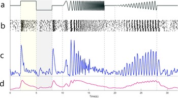
For light stimulation, we focused a developer module projector (DLP® LightCrafter 4500, Texas Instruments, Dallas, TX) through a custom light path of lens, mirror, and condenser onto the MEA. Stimulator intensity (as photoisomerization rate, P*/s/cone) was calibrated to match the previous Baden et al. (Reference Baden, Berens, Franke, Román Rosón, Bethge and Euler2016) study as closely as possible, with the white stimulus set to 3 × 10⁴ P*/s/cone photoisomerization rate for mouse UV- and M-cones and the black stimulus set to 104 P*/s/cone. A steady mean illumination 2 × 10⁴ P*/s/cone was present during, before, and after all electrical and visual stimuli to maintain adaptation state. Light stimuli included: full-field flash 2 s ON (white) and 2 s OFF (black); a chirp stimulus consisting of two sinusoidal intensity modulations (Fig. 2a), one with increasing frequency and one with increasing contrast; drifting 1000 × 300 μm bars with vertical bars at 15 locations, horizontal bars at 10 locations, and diagonal bars at 17 location for each diagonal axis, with the centers of adjacent bars separated by 200 μm; and full-field color flashes for 3 s each in a sequence of blue, black, green, and black.
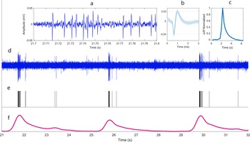
Sample raw data and equivalent pseudocalcium trace. (a) 100 ms of filtered voltage recording excerpted from (d). (b) Average of extracellular action potentials (mean ± s.d.). Dashed lines highlight baseline and peak. (c) OGB kernel. (d) 11 s sample of filtered data from an ON cell in response to the cycling flash stimulus. (e) Rastergram of spike times for this cell (note excluded spikes around 25 s assigned to a different cell). (f) Pseudocalcium trace produced by convolving the rastergram (e) with the OGB kernel (c).

Pseudocalcium trace generation for the chirp stimulus. (a) Stimulus brightness over time including 3 s ON and 3 s OFF full-field flash; gray, and two “chirps” composed of increasing frequency and increasing contrast respectively. (Vertical dashed lines separate various stimuli as well as the mean gray background). (b) Raster of spike times across multiple repetitions of the stimulus. (c) Peri-stimulus time histogram (PSTH) of these spike times across all trials using 100 ms time bins. (d) Pseudocalcium trace generated by convolving the rastergrams with the OGB kernel and averaging across trials.

Visual classification
In the reference study, algorithmic clustering was augmented with a few additional interventions that were not possible here. First, cells were originally separated based on direction selectivity to drifting bar stimuli. However, despite our best attempts at both replicating previous analysis and applying novel analyses we could not satisfactorily differentiate direction and orientation selective cells based on responses to our stimulus (see section “Discussion”). Nevertheless, we were still able to match cells from our dataset to each of the DS and OS clusters of the original report based solely on responses to the other stimuli. Second, alpha cells were originally discriminated based on soma size. Because we did not have imaging data for our recorded cells, we were unable to flag alpha cells in this way (clusters 6–8, 11–13, 33, and 34; see Fig. 3), although we were still able to use visual stimuli to match some alpha cells (clusters 11, 33, and 34). Third, because it can be difficult to discriminate amacrine cell (AC) and ganglion cell somas in calcium imaging, immunohistochemistry was used in the previous study to identify AC clusters. It is unlikely that we recorded spiking responses from ACs, but because this remains a slim possibility—despite their reputation as nonspiking cells—we matched our dataset to the full set of 75 cluster definitions including 26 AC clusters, as well as a 76th cluster for noisy cells. Few of our cells were best matched with an AC cluster with one exception noted in Results.
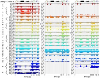
Average time varying calcium signals for the 49 RGC clusters reported in Baden et al. (Reference Baden, Berens, Franke, Román Rosón, Bethge and Euler2016) (left) average pseudocalcium signals for the spiking data assigned to these clusters from our present dataset (middle), and from an expanded dataset (right). Each trace was normalized to its respective peak. Value at left of each cluster is the percent of RGCs assigned to each cluster, rounded up. Clusters were combined to produce the 32 distinct RGC groups (indicated at far left), and loosely organized with OFF cells near the top, ON–OFF cells in the middle, and ON cells at the bottom. Vertical dashed lines separate stimuli from one another and from baseline responses to the mean gray background stimulus. The segments in order were: gray, white (ON), black (OFF), gray, frequency chirp, gray, contrast chirp, gray (and black), drifting bar, green, black, blue, and black.

As previously reported (Baden et al., Reference Baden, Berens, Franke, Román Rosón, Bethge and Euler2016), many individual RGC recordings were not sufficiently driven by the stimulus to support robust classification. Accordingly, we estimated how strongly the responses were driven by the stimulus by dividing the response variance across trials by the overall variance of responses. Spike counts were binned at 100 ms, response variance for each bin was calculated across at least 10 trials, and these values were then averaged. The overall variance was calculated across the full set of time bins and trials including both response intervals and spontaneous intervals. Cells with a response variance higher than the overall variance (a ratio higher than 1) were excluded from analysis as unreliably driven cells.
Finally, we projected the pseudocalcium traces of our visually responsive cells onto the lower-dimensional feature space previously determined by Baden et al. using sparse principal components analysis (sPCA). By using the sPCA features of the previous study, we ensured that our data was analyzed according to their definitions for cell clusters. We refer the reader to the earlier Baden et al. (Reference Baden, Berens, Franke, Román Rosón, Bethge and Euler2016) study for more extensive details on feature selection and clustering. These sPCA features included 20 features from the chirp, 8 features from the moving bar, 4 features from its temporal derivative, and 6 features from the color stimulus, yielding a 38-dimensional feature vector for each cell. Two features from a visual noise stimulus were excluded because very few of our cells produced significant receptive field maps in response to this stimulus. Classification was performed by calculating the Euclidean distance between the feature vector of each cell and the average feature vector of each cluster of reference dataset cells, assigning each cell to the most similar reference cluster.
Electrical stimulation
To calculate and examine the spike triggered average (STA) electrical preference of each cell group, we presented an electrical Gaussian noise stimulus with a mean of −800 mV and s.d. of 35% (280 mV) developed by Sekhar et al. (Reference Sekhar, Jalligampala, Zrenner and Rathbun2016). The duration of each pulse was set to 1 ms and the stimulation frequency was 25 Hz. The length of each trial of noise stimulation was 100 s; and from experiment to experiment the number of repetitions varied from 15 to 30. A stimulus generator (STG4000 Series; MCS, Reutlingen, Germany) was used for electrical stimulation. A LNP fitting toolbox (https://github.com/pillowlab/LNPfitting) (Williamson et al., Reference Williamson, Sahani and Pillow2015) was used to compute the STA of burst-corrected responses (Rathbun et al., Reference Rathbun, Ghorbani, Shabani, Zrenner and Hosseinzadeh2018) for each RGC. The STA can also be viewed as an estimate of the filter applied by the neuron to incoming stimuli—the electrical input filter.
Results
The intent of this study was to assess the possibility of assigning RGCs to predefined, putative types by converting their binary spiking data to pseudocalcium traces. Having assigned RGCs by type we hoped to then evaluate the electrical input filter (STA) of each type for use in retinal prosthetics.
We recorded the spiking responses of 892 mouse RGCs from nine retinas. For a stimulus-driven cell, the response variance should be lower than the overall variance, yielding a variance ratio less than 1. All cells with a variance ratio of 1 or higher were excluded, leaving 653 RGCs for classification.
Estimating calcium traces from spiking data
To convert our binary spiking data into pseudocalcium traces, each spike was convolved with the OGB kernel. Initially, we found that our traces were categorically more transient than those reported in Baden et al. We eventually realized that this strong discrepancy is the result of subthreshold calcium signals that are present in calcium imaging data but cannot be recorded in extracellular spiking data (Discussion). Reasoning that stimulus-driven spikes and subthreshold signals are strongly correlated, we doubled the duration of the OGB kernel as an imperfect but effective compensatory measure. This yielded a range of pseudocalcium response patterns much more similar to the reference calcium data. Fig. 1 shows an example of this conversion for a sample recording of flash stimulation responses. After comparing the classification results for both kernels, the doubled kernel was found to distribute data more broadly amongst the available groups rather than restricting assignment to only the most transient response groups. Therefore, this kernel was used for final clustering.
Classification
After converting binary spiking data to pseudocalcium traces, they were normalized similar to Baden et al. and each cell’s median across different trials was used (Fig. 2). Median traces were projected into a predefined feature space; and each cell was assigned to its most similar cluster. In the original study, responses were sorted into 75 distinct clusters. Clusters 1–39 were definitely RGCs; 40–49 were suspected RGCs; and 50–75 were ACs. For our analysis, one last cluster, number 76, contained all cells from the original study with noisy responses. Some of our data were best matched to this cluster and were subsequently disregarded. In the original study, sometimes multiple clusters were found to be subsets of distinct RGC groups and were therefore grouped together. Thus, the 49 RGC clusters yielded 32 distinct RGC groups. It was these 32 groups that we sought to assign to our new dataset through matching of the underlying clusters—as they represent an, admittedly provisional, scheme for classifying RGCs according to true physiological type. Fig. 3 shows the cluster means from the benchmark dataset (left column) as well as pseudocalcium means for our classified RGCs (middle and right). Our original experiments for pseudocalcium classification yielded 892 RGCs from nine retinas (Fig. 3, middle). In a follow-up experiment we used similar methods and were therefore able to increase this dataset to 2303 RGCs from 29 retinas (Fig. 3, right).
We found that 2303 stimulus-driven RGCs recorded from 29 retinas sorted into 29 of the 39 previously reported “certain” RGC clusters. Our RGCs also matched with 5 of the 10 “suspected” RGC clusters. Thus, 34 of the 49 RGC clusters (70%) were matched by our data. Clusters 76 (noisy responses) and 50–75 (displaced ACs) were omitted from the figure for clarity. When the 49 RGC clusters were merged to yield 32 functionally distinct RGC groups, our data was found to match 27 of the 32 groups (84%). Therefore, while we were able to assign cells from our recordings to most previously reported groups, some specific groups were not matched by our data (Discussion). Importantly, the mean cluster responses identified for 9 retinas remain largely the same as for 29 retinas. Each of the four new clusters constitutes only 1% or less of the dataset, resulting in noisy and unreliable cluster means. Overall, this indicates that these clusters are unlikely to change much with an increased dataset.
Estimating electrical input filters
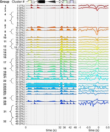
Previous work has shown that electrical input filter shapes vary according to coarsely defined RGC type (Sekhar et al., Reference Sekhar, Jalligampala, Zrenner and Rathbun2017; Ho et al., Reference Ho, Smith, Goetz, Lei, Galambos, Kamins, Harris, Mathieson, Palanker and Sher2018). Our goal in developing the present classification method was to examine nuanced distinctions between input filters (STAs) for the 32 different RGC groups. Fig. 4 shows cluster averages for all 792 RGCs from the larger dataset that had a statistically significant STA (as defined in Sekhar et al., Reference Sekhar, Jalligampala, Zrenner and Rathbun2016). In agreement with our previous work (Sekhar et al., Reference Sekhar, Jalligampala, Zrenner and Rathbun2017), OFF clusters as defined in the Baden study (1, 2, 10, and 11) have downward deflections directly to the left of time zero in their electrical STAs. Likewise, most ON clusters (21, 22, 24–31, 33, 35, and 40) have upward deflections; although clusters 23 and 37 are downward and 34, 36, and 41 are difficult to determine. It appears that most ON–OFF clusters also have downward deflections (14–20) reflecting a stronger OFF input as seen in the flash response. While these population averages demonstrate modest success for the present pseudocalcium classification technique, we also found STA diversity within RGC groups that suggest remaining inadequacies in classification. This issue will be addressed in detail in a subsequent study.
Response of classified cells to electrical noise stimulus. (left) Cluster averages for only the cells with significant electrical STAs, taken from Fig. 3, right. (Order of visual stimuli is as in Fig. 3). (right) Electrical STAs averaged across all cells assigned to the cluster. For each STA, horizontal line represents the stimulus mean of −800 mV. Traces above this line indicate that stimuli preceding spikes were on average a higher (less negative) voltage, traces below the line reflect more negative voltages. STA amplitudes were scaled to show detail. Traces to the right of time zero reflect the variation of random noise.

Discussion
Our main concern was to classify mouse RGCs to one of 32 proposed RGC types described in the catalog of Baden et al. (Reference Baden, Berens, Franke, Román Rosón, Bethge and Euler2016). In order to match our extracellular spiking activity with their calcium imaging-based clustering data, we transformed RGC spike responses into pseudocalcium traces. Of their 32 groups, 27 were matched by our data. In support of our work in bionic vision, these RGCs were also presented with an electrical noise stimulus (Sekhar et al., Reference Sekhar, Jalligampala, Zrenner and Rathbun2016). The resultant STAs have been previously shown to vary with coarsely defined RGC type (Sekhar et al., Reference Sekhar, Jalligampala, Zrenner and Rathbun2017; Ho et al., Reference Ho, Smith, Goetz, Lei, Galambos, Kamins, Harris, Mathieson, Palanker and Sher2018). In surveying the STAs of our 27 matched groups, we found some evidence to suggest group-specific filters, however, many groups contained multiple filter shapes. Given known inadequacies in classification, elaborated below, we cannot yet discount the possibility that many RGC groups might possess unique input filters; however, the present results are unable to convincingly support or reject that hypothesis.
On putative RGC type catalogs
Many authors have recently attempted to collect all known and heretofore unknown RGC types into a single visual response classification scheme (Bae et al., Reference Bae, Mu, Kim, Turner, Tartavull, Kemnitz, Jordan, Norton, Silversmith, Prentki, Sorek, David, Jones, Bland, Sterling, Park, Briggman and Seung2018; Jouty et al., Reference Jouty, Hilgen, Sernagor and Hennig2018; Rheaume et al., Reference Rheaume, Jereen, Bolisetty, Sajid, Yang, Renna, Sun, Robson and Trakhtenberg2018; Tran et al., Reference Tran, Shekhar, Whitney, Jacobi, Benhar, Hong, Yan, Adiconis, Arnold, Lee, Levin, Lin, Wang, Lieber, Regev, He and Sanes2019). Accordingly, the study of Baden et al. on which we have based our work is no longer the most complete or definitive. Nevertheless, it was one of the first reasonably complete attempts; and so we have anchored the present work on it for better or worse. It is likely that some of the mixed electrical filters reported here may result from incompletely differentiated types in the underlying classification scheme. To resolve the issue, we must refine our methods so that our data can be classified against the most complete schemes available. At present, we find the spike train metrics of Jouty et al. to be quite compelling and although Bae et al. appears to be a remarkably complete classification scheme, it remains unclear how to achieve such classification solely with visual response spike trains. Our group has already moved on to type definitions intrinsic to spike trains on which we will report shortly. Nevertheless, in undertaking this work we were surprised to find few references in the literature to the type of pseudocalcium approach we have taken here—despite its self-evident nature. Likely many others have met with similar disappointment and opted not to share their learned experience. Therefore, in recognizing the utility of so-called negative results, this paper has been submitted to establish such a record.
Subthreshold calcium signals
Although the pseudocalcium method matched our data to most of the RGC groups reported in Baden et al. (Reference Baden, Berens, Franke, Román Rosón, Bethge and Euler2016), it failed to match all groups. Many of our RGC clusters also had shorter chirp response durations than their reference clusters (e.g., 10 and 29). Consequently, our data failed to match the most sustained clusters (e.g., 3–9, 12–13, 22, 31–32, 38–39, and 42–49). We interpret this to arise from strong subthreshold calcium signals that do not translate into spikes for higher frequencies or lower contrasts. Indeed, calcium signals are known to correspond to subthreshold events like excitatory postsynaptic potentials that are seldom detected in MEA recordings (Nakajima & Baker, Reference Nakajima and Baker2018). We therefore suspect that many of our cells that should have been matched to sustained groups were misclassified as more transient groups.
Direction selectivity
Direction selectivity is well documented (Briggman et al., Reference Briggman, Helmstaedter and Denk2011); and so it is frustrating that our data failed to yield sufficient multimodality in direction selectivity measures. We attribute this result to the stimulus adaptations that were necessary to support MEA recording. As described in Methods, we replaced the 8 drifting bars that are typically used with 118 bars that drifted along the electrode array to ensure that all eight directions were presented to any possible recording location. Because these drifting bars were seldom centered on a recorded RGC, the ~3 bars of each direction that most directly crossed a cell’s receptive field were used—resulting in imperfect response estimates. Additionally, with only five repetitions for any given bar stimulus, it appears that our firing response estimates were too noisy. Nevertheless, remaining visual responses were sufficient to assign cells from our dataset to each of the DS and OS groups.
Alpha cells
One category of RGC type that we often failed to match was alpha cells. In the Baden study, alpha cells were identified based on soma size. Because our MEA recordings did not allow us to measure soma size, we failed to match five of six OFF alpha clusters, leading to two unmatched OFF groups. Nevertheless, we did match data to one OFF and the two ON alpha groups, using only visual responses.
Missing ON cells
A hallmark of the original Baden study was that none of the 49 RGC clusters accounted for more than 5% of the overall RGC population with the vast majority only containing 1 or 2% of the population. In contrast, classification of our data resulted in many clusters receiving no assignments and others receiving well over 5% and up to 16%. This likely is the result of our more transient chirp responses resulting in many ON cells (clusters 3–9) being assigned to ON–OFF clusters (clusters 14–18). This suspected misclassification is understandable considering that the ON clusters of Baden et al. also had significant onset and offset responses (ON–OFF-like behavior) to the drifting bar stimulus.
Notably, the “ON sustained” group 22 (clusters 31 and 32) was largely absent in our classified data; whereas, we found that 17% of our RGCs (110 cells) were assigned to group 38 (clusters 58, 59, and 60)—one of the ON sustained AC groups. In the original Baden et al. study, ACs, like alpha cells, were also reclustered—this time based on immunohistochemistry labeling. Because we cannot fully rule out spiking AC signals from our dataset, we included the AC clusters (50–75) in assigning our RGC data even though recording of extracellular AC spiking responses is expected to be exceedingly rare compared to calcium imaging of AC responses. We suspect, however that these group 38 cells were misclassified and are actually group 22 RGCs. Beyond these, only 14 other RGCs were assigned to AC clusters (50–75).
Spikes versus calcium signals for classification
Both calcium signals and spike trains have their relative advantages and disadvantages for the purposes of classifying RGCs. In common, both methods reflect the stimulus-modulated spiking rate. While calcium signals provide additional information about subthreshold events, spike trains provide more precise timing information. The degree to which information from these sources is redundant versus independent, and the degree to which this information can be used in RGC type classification remains to be determined.
Ideally, high-quality calcium recordings simultaneous with MEA recordings would maximize information for high-throughput RGC classification. This would also better connect spike trains with calcium signals. Many labs including ours, however, lack either the resources or expertise to execute such an approach, or are investigating experimental questions that preclude this approach. A worthy goal toward which many are working is to develop methods to infer between calcium and spike train data. Although there is a lack of proper solutions for reconstructing calcium signals from spike traces, many algorithms have been developed for the inverse estimation of spike activity from neuronal calcium imaging. Examples of such approaches include template-matching (Greenberg et al., Reference Greenberg, Houweling and Kerr2008), deconvolution techniques (Grewe et al., Reference Grewe, Langer, Kasper, Kampa and Helmchen2010) and approximate Bayesian inference (Deneux et al., Reference Deneux, Kaszas, Szalay, Katona, Lakner, Grinvald, Rózsa and Vanzetta2016). For the inverse problem, inferring calcium data from spike trains has received relatively little discussion in the literature. The present work appears to be one of the relatively few examples where the calcium kernel has been used in the opposite direction to infer calcium traces from known spike trains. Due to limited work on this problem, the two complementary methods of MEA and calcium recording, and their resultant knowledge domains continue to be relatively siloed from one another. We hope that our open discussion of our difficulties in this realm might help others to break through this barrier.
Connecting healthy and blind retinal electrophysiology for bionic vision
Finally, connecting electrical responsiveness data from the healthy mouse retina to the blind retina remains a difficult unresolved problem in our field. Our group has typically taken the approach of working first in the healthy retina to develop new methods because healthy tissue has a significantly higher yield of useful data per animal. That said, we have also performed experiments similar to those described here in intermediate and fully blind mouse retinas. We are pursuing preliminary evidence that electrical response properties themselves may be an effective way to classify RGCs according to visual type in the blind retina. Much more work remains in this area and both the Rathbun and Hosseinzadeh labs are actively expanding their patch clamping abilities to better understand how electrical responses can be used to identify RGC types in the blind retina. Our work will prove useful not only in blind retina research, but in bidirectional bionic vision implants where recordings from the electrode array can be used to map out the “labeled lines” of the underlying cells so that the “correct” visual information is delivered to each cell.
Data availability statement
The data that support the findings of this study are openly available in Zenodo at http://doi.org/10.5281/zenodo.4462320.
Acknowledgments
We thank Prof. Thomas Euler, Prof. Philip Berens, and Master Yannik Bauer for their guidance in understanding the reference paper. This project was built upon the Master’s thesis work of Mahdi Sadeghi.
Author contributions
D.L.R. and Z.H. are shared last authors. H.S. and Z.H. performed the experiments. H.S., E.Z., D.L.R., and Z.H. interpreted the results. H.S., D.L.R., and Z.H. designed the study and drafted the manuscript. All authors corrected and approved the final version of the manuscript.
Funding statement
This work was supported by the Deutsche Forschungsgemeinschaft (HO 6221/1-1) to Z.H., by the Bundesministerium für Bildung und Forschung (031a308) to D.L.R., and by the Tistou and Charlotte Kerstan Foundation to Z.H.
Competing interest
The authors have no competing interest to declare.