1 Introduction
Cavitation bubbles expanding and shrinking near rigid boundaries move towards the boundary due to the action of the secondary Bjerknes force (Blake & Gibson Reference Blake and Gibson1987; Best & Kucera Reference Best and Kucera1992). The oscillating flow near the wall creates naturally a strong and unsteady boundary layer flow with high shear rates. Additionally, the radial flow is accompanied by a jetting flow accelerating liquid to impinge on and spread along the wall.
Historically, the shear stress generated from steady impinging jets on solid walls has been solved by Glauert (Reference Glauert1956), and confirmed through simulations (Deshpande & Vaishnav Reference Deshpande and Vaishnav1982; Phares, Smedley & Flagan Reference Phares, Smedley and Flagan2000) and experiments (Narayanan, Seyed-Yagoobi & Page Reference Narayanan, Seyed-Yagoobi and Page2004; Visser et al. Reference Visser, Gielen, Hao, Le Gac, Lohse and Sun2015). However, the shear stress produced by transient jets from near-wall cavitation has recently received more attention, in particular for its importance for surface cleaning (Ohl et al. Reference Ohl, Arora, Dijkink, Janve and Lohse2006a ; Kim et al. Reference Kim, Kim, Choi and Kim2009; Gonzalez-Avila et al. Reference Gonzalez-Avila, Huang, Quinto-Su, Wu and Ohl2011) and cell membrane poration cells (Ohl et al. Reference Ohl, Arora, Ikink, De Jong, Versluis, Delius and Lohse2006b ; Le Gac, Zwaan & Ohl Reference Le Gac, Zwaan, van den Berg and Ohl2007). Very few experiments have tried to measure the wall shear stress. Dijkink & Ohl (Reference Dijkink and Ohl2008) combined high-speed photography with a hot-film anemometer and found short peaks with stress amplitudes of up to 3.5 kPa occurring right after the jet impact. Given the limited temporal bandwidth of their device, the maximum shear stress reported may only be a lower bound. Their sensor can only measure at a single location. Thus, to map spatial stress requires many measurements with identical bubbles, which is difficult to achieve. To fill this knowledge gap, we present here a numerical approach to estimate the wall shear stress. It is based on the finite-volume method (FVM) to discretize the fluid domain and the volume-of-fluid (VOF) method to capture the bubble–water interface. We can reliably simulate the bubble dynamics through the first and second collapse and obtain a spatio-temporal map of the wall shear stress.
This work is organized as follows. First, we verify the numerical model with experiments and previous shear stress measurement from Dijkink & Ohl (Reference Dijkink and Ohl2008). Then we study the flow field details near the boundary to clarify the flow features that lead to the wall shear stress. After that, a spatio-temporal map of the wall shear stress distribution is presented and discussed. A test of our numerical method against previous works and an analytic solution is provided in the appendix.
2 Methodology
Here we resolve the shear flow produced by a cavitation bubble collapsing near a solid boundary in water. The flow field is obtained by solving the compressible Navier–Stokes (NS) equations and capturing the gas–water interface with the VOF method based on the finite-volume framework of OpenFOAM (Weller et al. Reference Weller, Tabor, Jasak and Fureby1998). The flow is dominated mostly by inertia of the liquid and the compressibility of the gas; the viscosity is only important close to the surface. For simplicity, we model the initial (laser-created) cavitation bubble consisting of non-condensable gas starting from a small volume at high pressure. The sharp interface of the cavitation bubble is captured by solving the transport equation for the volume fraction of the liquid (Miller et al. Reference Miller, Jasak, Boger, Paterson and Nedungadi2013; Koch et al. Reference Koch, Lechner, Reuter, Köhler, Mettin and Lauterborn2016):
 $$\begin{eqnarray}\displaystyle & \displaystyle {\displaystyle \frac{\unicode[STIX]{x2202}\unicode[STIX]{x1D6FC}}{\unicode[STIX]{x2202}t}}+\unicode[STIX]{x1D735}\boldsymbol{\cdot }(\unicode[STIX]{x1D6FC}\boldsymbol{u})+\unicode[STIX]{x1D735}\boldsymbol{\cdot }(\unicode[STIX]{x1D6FC}(1-\unicode[STIX]{x1D6FC})\boldsymbol{U}_{\boldsymbol{r}})=\unicode[STIX]{x1D6FC}(1-\unicode[STIX]{x1D6FC})\left({\displaystyle \frac{\unicode[STIX]{x1D713}_{g}}{\unicode[STIX]{x1D70C}_{g}}}-{\displaystyle \frac{\unicode[STIX]{x1D713}_{l}}{\unicode[STIX]{x1D70C}_{l}}}\right){\displaystyle \frac{\text{D}p}{\text{D}t}}+\unicode[STIX]{x1D6FC}\unicode[STIX]{x1D735}\boldsymbol{\cdot }\boldsymbol{u}, & \displaystyle\end{eqnarray}$$
where
 $\unicode[STIX]{x1D6FC}$
is the volume fraction of the liquid phase,
 $\boldsymbol{u}$
is the velocity field,
 $p$
is the pressure and
 $\boldsymbol{U}_{\boldsymbol{r}}$
is the relative velocity between the two phases, which helps to ensure a sharp interface (Rusche Reference Rusche2003). Compressibility is included on the right-hand side, which contains the compressibility of both phases (liquid and gas) with
 $\unicode[STIX]{x1D713}=\text{D}\unicode[STIX]{x1D70C}/\text{D}p$
from the equation of state (EOS). For the gas phase a polytropic EOS is used, while for the liquid phase the Tait EOS (MacDonald Reference MacDonald1969) is applied, similar to the cavitation bubble simulations in Koch et al. (Reference Koch, Lechner, Reuter, Köhler, Mettin and Lauterborn2016) and Koukouvinis et al. (Reference Koukouvinis, Gavaises, Supponen and Farhat2016a
,Reference Koukouvinis, Gavaises, Supponen and Farhat
b
).
In the compressible NS equations, we use the single-field formulation and treat the two phases as a compressible and immiscible Newtonian fluid while neglecting the heat and mass transfer:
 $$\begin{eqnarray}\displaystyle & \displaystyle {\displaystyle \frac{\unicode[STIX]{x2202}\unicode[STIX]{x1D70C}}{\unicode[STIX]{x2202}t}}+\unicode[STIX]{x1D735}\boldsymbol{\cdot }(\unicode[STIX]{x1D70C}\boldsymbol{u})=0, & \displaystyle\end{eqnarray}$$
 $$\begin{eqnarray}\displaystyle & \displaystyle {\displaystyle \frac{\unicode[STIX]{x2202}\unicode[STIX]{x1D70C}\boldsymbol{u}}{\unicode[STIX]{x2202}t}}+\unicode[STIX]{x1D735}\boldsymbol{\cdot }(\unicode[STIX]{x1D70C}\boldsymbol{u}\boldsymbol{u})=-\unicode[STIX]{x1D735}p+\unicode[STIX]{x1D735}\boldsymbol{\cdot }\unicode[STIX]{x1D668}+\boldsymbol{f}_{\unicode[STIX]{x1D739}}, & \displaystyle\end{eqnarray}$$
where
 $\unicode[STIX]{x1D70C}$
is the density of the fluid and
 $\unicode[STIX]{x1D668}$
is the viscous stress tensor, which is calculated as
 $\unicode[STIX]{x1D668}=\unicode[STIX]{x1D707}(\unicode[STIX]{x1D735}\boldsymbol{u}+\unicode[STIX]{x1D735}\boldsymbol{u}^{\text{T}}-2/3(\unicode[STIX]{x1D735}\boldsymbol{\cdot }\boldsymbol{u})\unicode[STIX]{x1D644})$
, with the dynamic viscosity
 $\unicode[STIX]{x1D707}$
and the identity tensor
 $\unicode[STIX]{x1D644}$
. In (2.3)
 $\boldsymbol{f}_{\unicode[STIX]{x1D739}}$
is the source term due to surface tension, which is modelled with the continuous-surface-force (CSF) method (Brackbill, Kothe & Zemach Reference Brackbill, Kothe and Zemach1992). Flow properties are calculated based on the volume fraction of the liquid, with
 $\unicode[STIX]{x1D701}=\unicode[STIX]{x1D701}_{l}\unicode[STIX]{x1D6FC}+\unicode[STIX]{x1D701}_{g}(1-\unicode[STIX]{x1D6FC})$
, where
 $\unicode[STIX]{x1D701}_{l}$
and
 $\unicode[STIX]{x1D701}_{g}$
are physical properties of the liquid and the gas.
We verify the numerical method by comparing the simulation results with experiments. In the experiment, cavitation bubbles are created with a 6 ns duration pulse from a Q-switched laser (New Wave,
 $\unicode[STIX]{x1D706}=532~\text{nm}$
), which is focused at a distance
 $h$
close to a wall. The bubble dynamics is recorded with a high-speed camera (Photron SAX-2, Japan) operating at 200 000 frames per second (293 ns exposure time). The high-speed recorded images with pixel size of
 $20~\unicode[STIX]{x03BC}\text{m}$
are used to validate the gas-phase dynamics and thus the flow field in the numerical simulations. For the validation of the wall shear stress from the simulations, we benchmarked the model with earlier simulations of a submerged steady wall jet impinging on a surface Deshpande & Vaishnav (Reference Deshpande and Vaishnav1982); see appendix. We also compare the simulation result with experiments (Dijkink & Ohl Reference Dijkink and Ohl2008) of cavitation-bubble-induced wall shear stress. To simplify the simulation, an axisymmetric domain is chosen, with a size of 5 mm in radial and 10 mm in axial directions. The computational mesh contains 101 grid points in radial direction and 201 grid points in axial direction initially. These are refined recursively four times. In the area of interest, i.e. where the bubble is located, the cell size is approximately
 $3~\unicode[STIX]{x03BC}\text{m}$
wide. For the solid boundary, a no-slip condition is used. In the near-boundary region, the mesh is further refined recursively down to a spacing
 $\unicode[STIX]{x0394}x=0.05~\unicode[STIX]{x03BC}\text{m}$
, to resolve a linear increasing velocity within the thin boundary layer.
3 Results
3.1 Comparison with experiments
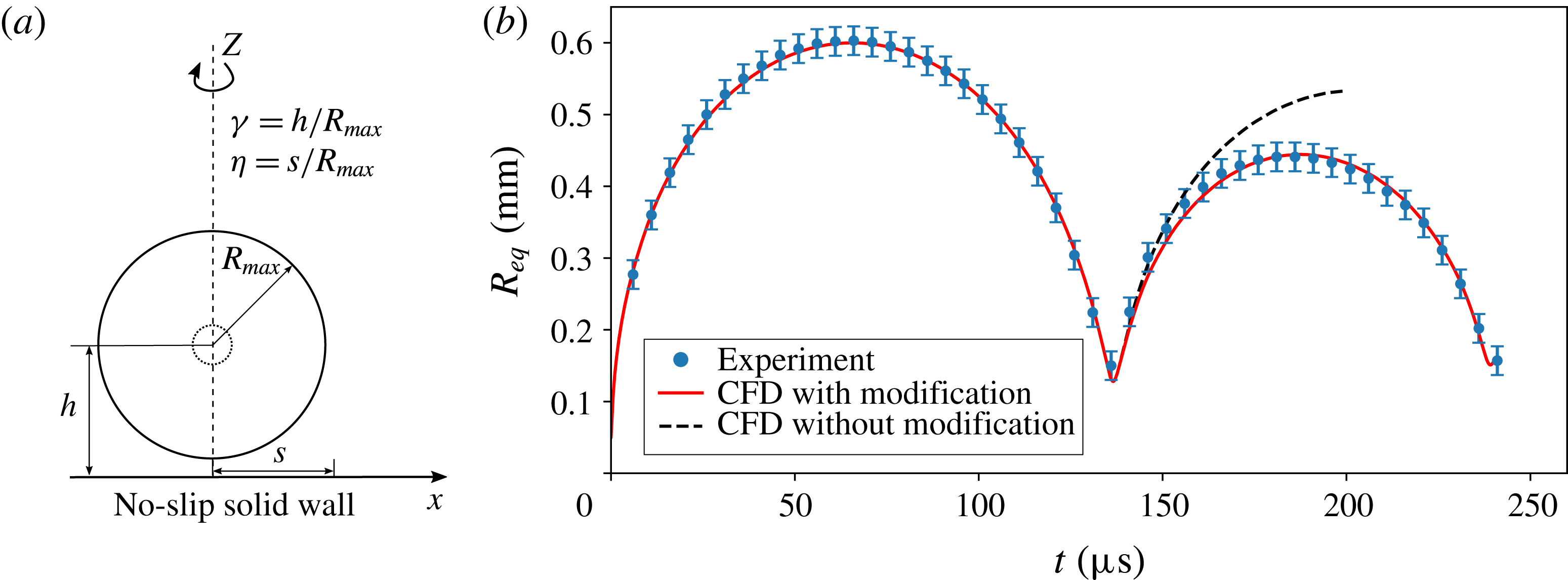
(a) Sketch of the problem and parameters. The dashed circle is the bubble nucleation and the solid circle is the bubble at maximum size. (b) Comparison of the equivalent spherical bubble radius from simulations (lines) with the experiment (filled symbols). The dashed line shows the result using a constant polytropic exponent of
 $\unicode[STIX]{x1D705}=1.4$
; and the red solid line represents the result using a polytropic exponent of
 $\unicode[STIX]{x1D705}=1.4$
from
 $t=0~\unicode[STIX]{x03BC}\text{s}$
to
 $t=136.5~\unicode[STIX]{x03BC}\text{s}$
and a higher polytropic exponent of
 $\unicode[STIX]{x1D705}_{2}=2.4$
from
 $t=136.5~\unicode[STIX]{x03BC}\text{s}$
. The error bar presents the uncertainty from the recorded images.

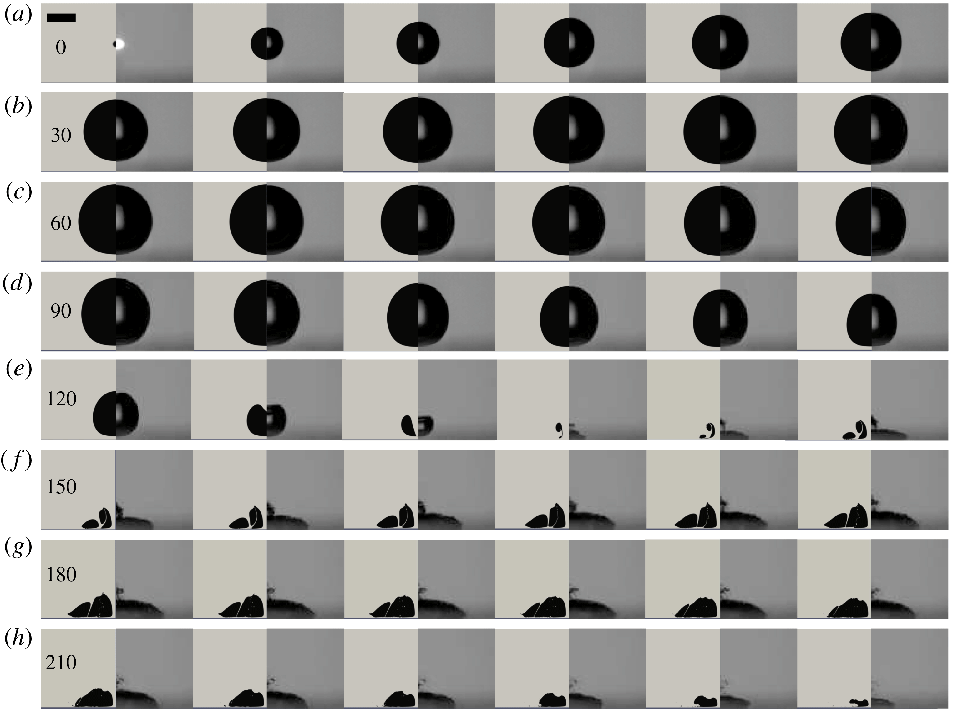
Comparison of bubble shape evolution for stand-off distance
 $\unicode[STIX]{x1D6FE}=1.1$
. The left part in a single frame is the simulation result, while the right part is the experimental result. The time of the first frame in each row is indicated in
 $\unicode[STIX]{x03BC}$
s, the inter-frame time is
 $5~\unicode[STIX]{x03BC}\text{s}$
, and the scale bar represents 0.5 mm. The boundary is below each frame.

Before we have a detailed look into the flow near to the boundary and the wall shear stress generated, we compare the overall bubble dynamics together with the snapshots of the bubble shape. Figure 1(a) shows the sketch of the problem and introduces the coordinates of the axisymmetric problem. Figure 1 compares the volume-equivalent spherical bubble radius between the experiment (filled symbols,
 $R_{max}=0.6~\text{mm}$
,
 $\unicode[STIX]{x1D6FE}=1.1$
) and the simulations (lines). In the simulations and the experiments, the bubble due to the high pressure inside expands in the initially stagnant liquid. By adjusting this pressure while keeping the radius,
 $R(t=0)=50~\unicode[STIX]{x03BC}\text{m}$
, constant, we can achieve good agreement for the expansion stage to an almost spherical bubble and the later shrinkage. Yet, after re-expansion, we find a considerable deviation of the equivalent bubble radius between the experiment and a straightforward simulation (dashed line); the bubble after collapse expands much larger in the simulations. We attribute this difference to the cushioning effect of the gas during the collapse: the non-condensable gas slows down the last stage of the collapse, resulting in less energy being lost from acoustic radiation and viscous damping, hence allowing for a larger re-expansion. To deal with this discrepancy, while not modelling the mass transfer, Lee, Klaseboer & Khoo (Reference Lee, Klaseboer and Khoo2007) implemented an experimental correlation accounting for the energy loss during the collapse into their boundary integral method based on data from Cole (Reference Cole1965). Wang (Reference Wang2014) also considered the energy loss due to shock-wave emission during the early expansion stage and the late bubble collapse and uses the bubble wall Mach number as a criterion. Both methods achieved reasonable agreement with experimental results; however, they are difficult to implement consistently in the present VOF framework. Here we provide an alternative approach by increasing the polytropic exponent of the gas after the collapse. This effectively removes internal energy from the bubble and the bubble expansion is reduced, although the mass transfer is not modelled. The new polytropic exponent is found by fitting the experimental second re-expansion to the simulation; see solid line in figure 1. Here we use for the polytropic exponent during the initial expansion and collapse
 $\unicode[STIX]{x1D705}=1.4$
and later
 $\unicode[STIX]{x1D705}=2.4$
. The increase of
 $\unicode[STIX]{x1D705}$
at the bubble rebound indicates the energy loss of the bubble at the collapse, i.e. less energy of the bubble is converted to kinetic energy of the flow after its rebound. This energy loss is
 $\unicode[STIX]{x1D6FE}$
-dependent (Vogel & Lauterborn Reference Vogel and Lauterborn1988; Vogel, Lauterborn & Timm Reference Vogel, Lauterborn and Timm1989). By comparing the simulations and experimental results, we find that
 $\unicode[STIX]{x1D705}=2.4$
after the first collapse models sufficiently well the energy loss for
 $\unicode[STIX]{x1D6FE}\approx 1$
.
Figure 2 compares the computed bubble dynamics (left part of each frame) with the experiments (right part of each frame). The rigid boundary for the experiment and the simulation is located at the bottom of each frame. At time
 $t=0$
the bubble is nucleated. In the simulation, the bubble starts with a spherical nucleus
 $R(t=0)=50~\unicode[STIX]{x03BC}\text{m}$
containing gas at a pressure of
 $p_{g}(t=0)=1300$
bar, while the bright spot in the experiment is due to the plasma emission from the dielectric breakdown. Although the complex plasma and fluid dynamics of the nucleation is ignored, already at frame
 $t=5~\unicode[STIX]{x03BC}\text{s}$
very good agreement of the expansion dynamics is obtained. After an expansion of the bubble to a maximum volume of an approximate sphere with radius
 $R(t=70~\unicode[STIX]{x03BC}\text{s})=0.6~\text{mm}$
, the bubble shrinks and develops a jet flow towards the boundary before reaching its minimum volume at
 $t\approx 135~\unicode[STIX]{x03BC}\text{s}$
. During re-expansion a rather complex bubble shape is observed; the bubble separates into a pancake shape close to the boundary and small fragments higher up along the axis of symmetry. The simulations reveal a second splitting at
 $t=145~\unicode[STIX]{x03BC}\text{s}$
and reconnection of the flat bottom part when the bubble volume shrinks again, e.g. from
 $t=210~\unicode[STIX]{x03BC}\text{s}$
. Till the second collapse we find good agreement of the outer shape of the bubble between simulation and experiment. Please keep in mind that the simulation shows a cut through the fluid domain while the high-speed recording are a photographic projection of the bubble.
Next we present a comparison of the wall shear stress at one position on the boundary with a measurement of Dijkink & Ohl (Reference Dijkink and Ohl2008) for the cavitation bubble at a stand-off
 $\unicode[STIX]{x1D6FE}=1.0$
. For this we have to approximate the wall shear stress as
 $$\begin{eqnarray}\displaystyle \unicode[STIX]{x1D749}=\unicode[STIX]{x1D707}\!\left.{\displaystyle \frac{\text{d}\boldsymbol{u}_{\boldsymbol{r}}}{\text{d}y}}\right|_{y=0}\approx \unicode[STIX]{x1D707}\!\left.{\displaystyle \frac{\boldsymbol{u}_{\boldsymbol{r}}(y)}{y}}\right|_{y\leqslant \unicode[STIX]{x1D716}}, & & \displaystyle\end{eqnarray}$$
where
 $\boldsymbol{u}_{\boldsymbol{r}}$
is the flow velocity component parallel to the wall,
 $y$
is the distance to the boundary, and
 $\unicode[STIX]{x1D716}$
is the thickness of the region with constant shear rate which is located within the boundary layer (Schlichting et al.
Reference Schlichting, Gersten, Krause and Oertel1955; Visser et al.
Reference Visser, Gielen, Hao, Le Gac, Lohse and Sun2015). To validate the calculation by (3.1), we perform a simulation of the steady submerged wall jet and compare the results with Glauert’s (Reference Glauert1956) analytical solution and the classical simulation from Deshpande & Vaishnav (Reference Deshpande and Vaishnav1982); see appendix. The comparisons indicate that the calculation of the wall shear stress with the present model is reliable once the region with constant shear rate within the boundary layer is resolved.
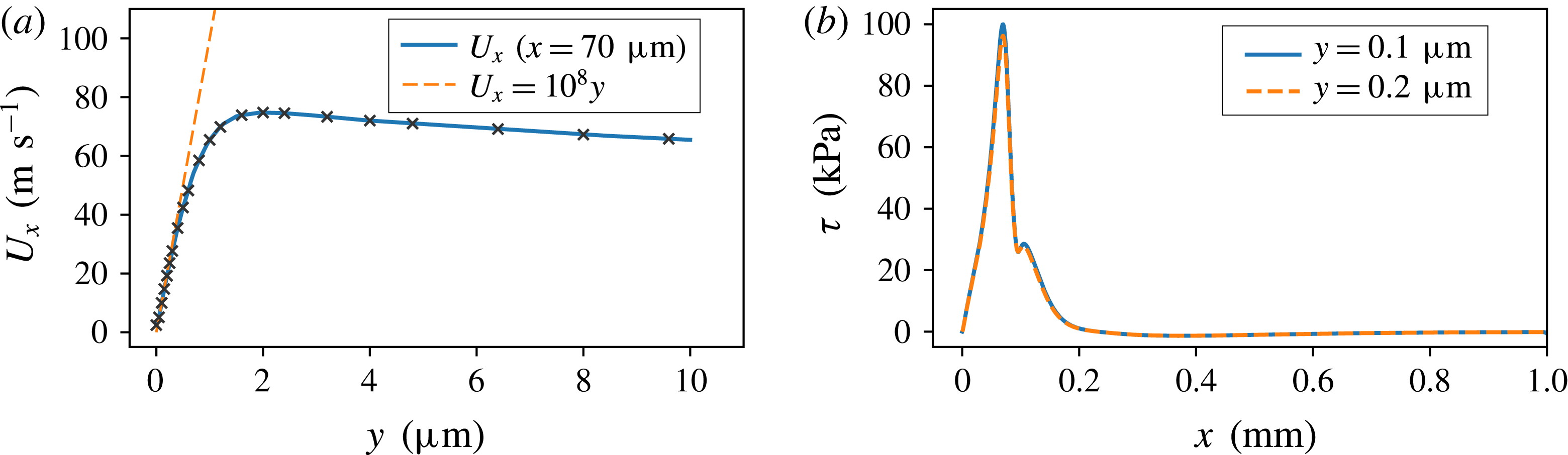
Flow and wall shear stress at
 $t=133~\unicode[STIX]{x03BC}\text{s}$
for the bubble of
 $\unicode[STIX]{x1D6FE}=1.0$
. (a) The radial velocity distribution along the vertical direction within the boundary layer at
 $x=70~\unicode[STIX]{x03BC}\text{m}$
. Radial velocity
 $U_{x}$
is linear with a slope of
 $10^{8}$
when
 $y<0.4~\unicode[STIX]{x03BC}\text{m}$
; the crosses represent the grid points within the boundary layer. (b) The wall shear stress distribution along boundary calculated at
 $y=0.1~\unicode[STIX]{x03BC}\text{m}$
and
 $y=0.2~\unicode[STIX]{x03BC}\text{m}$
.

Before we compare the wall shear stress reproduced by this model to the measurement of Dijkink & Ohl (Reference Dijkink and Ohl2008) for the cavitation bubble at a distance of
 $\unicode[STIX]{x1D6FE}=1.0$
, we look for the boundary layer formed by the spreading of the liquid jet induced by a collapsing bubble to determine the minimum
 $\unicode[STIX]{x1D716}$
. Figure 3(a) shows the vertical distribution of the radial velocity
 $U_{x}$
at
 $t=133~\unicode[STIX]{x03BC}\text{s}$
and
 $x=70~\unicode[STIX]{x03BC}\text{m}$
, where the largest shear occurs (see figure 6). The crosses indicate the positions of the resolved cells close to the boundary. We obtain a constant slope greater than 5 and more cells demonstrating sufficient resolution to resolve the constant shear near the boundary with a thickness of approximately
 $1.5~\unicode[STIX]{x03BC}\text{m}$
. For
 $y<0.4~\unicode[STIX]{x03BC}\text{m}$
,
 $U_{x}$
is linear with
 $y$
with a shear rate of
 $10^{8}~\text{s}^{-1}$
, i.e. the minimum
 $\unicode[STIX]{x1D716}\approx 0.4~\unicode[STIX]{x03BC}\text{m}$
. As a proof that this holds for all the calculations, we plot in figure 3(b) the wall shear stress distribution as a function of
 $x$
using (3.1) with
 $y=0.1~\unicode[STIX]{x03BC}\text{m}$
and
 $y=0.2~\unicode[STIX]{x03BC}\text{m}$
. The agreement demonstrates that the stresses are fully resolved even at locations of highest shear. In the remaining calculations, we use
 $y=0.1~\unicode[STIX]{x03BC}\text{m}$
.
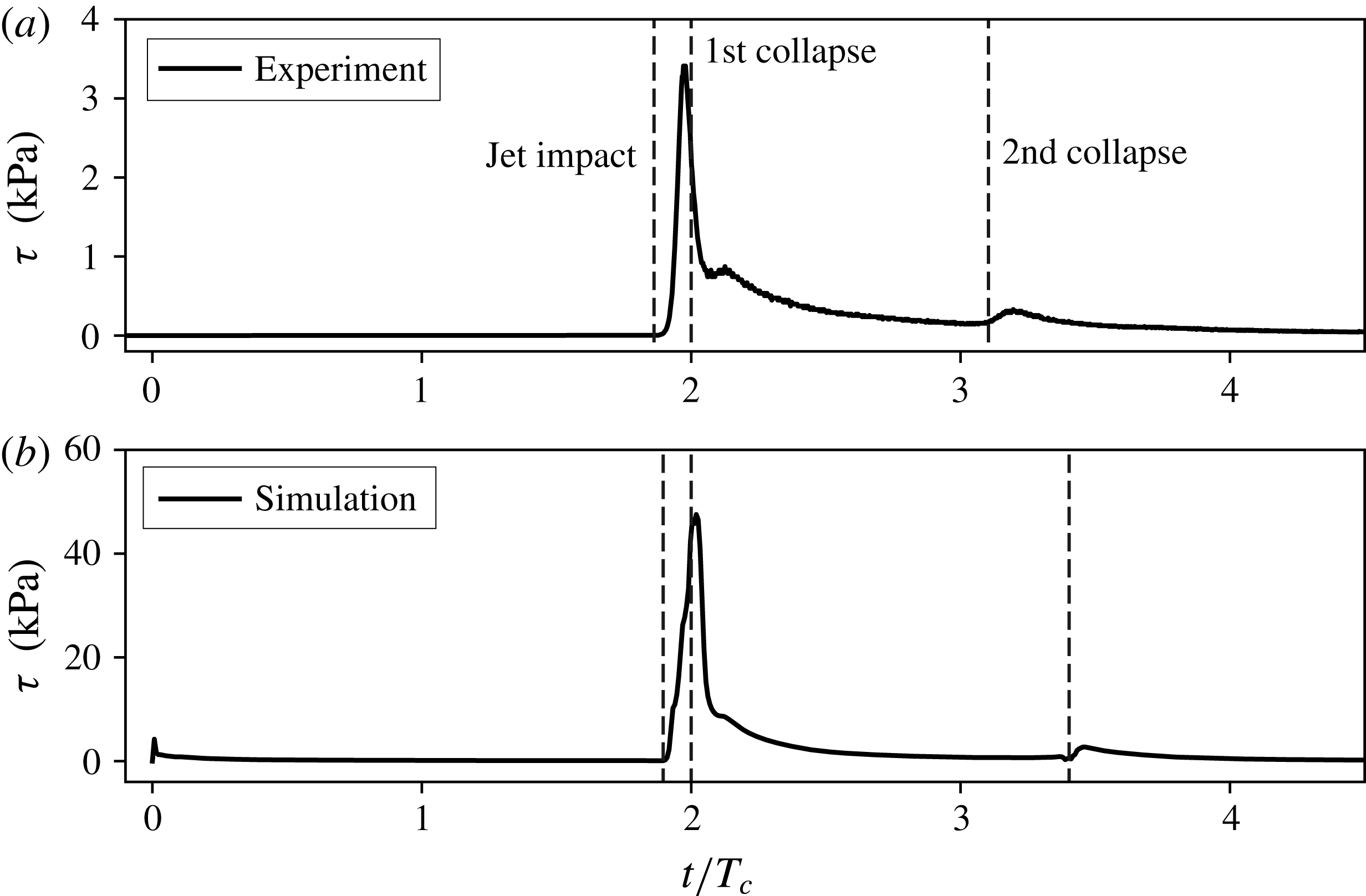
Comparison of measured and simulated wall shear stress at a non-dimensional distance of
 $\unicode[STIX]{x1D702}=0.33$
from the boundary for a bubble at a distance of
 $\unicode[STIX]{x1D6FE}=1.0$
: (a) the experimental result from Dijkink & Ohl (Reference Dijkink and Ohl2008); (b) the calculation from the current study. The horizontal axis is the dimensionless time normalized by the collapse time
 $T_{c}$
, and the vertical axis is the wall shear stress in kPa. The dashed lines in each plot represent the instances of jet impact, first collapse and second collapse, respectively. The jet impact occurs before the bubble reaches its minimum volume. Also note that, in experiments,
 $R_{max}\approx 750~\unicode[STIX]{x03BC}\text{m}$
and
 $T_{c}\approx 80~\unicode[STIX]{x03BC}\text{s}$
; in simulations,
 $R_{max}\approx 600~\unicode[STIX]{x03BC}\text{m}$
and
 $T_{c}\approx 69~\unicode[STIX]{x03BC}\text{s}$
.

Figure 4 compares the measured and simulated wall shear stresses recorded at
 $\unicode[STIX]{x1D702}=0.33$
(
 $\unicode[STIX]{x1D702}=s/R_{max}$
, where
 $s$
is the distance to the axis of symmetry) at a stand-off parameter of
 $\unicode[STIX]{x1D6FE}=1.0$
. The horizontal axis is the time normalized by the collapse time
 $T_{c}$
, while the vertical axis is the measured and calculated wall shear stresses in kPa. In the simulations we have accounted for the imperfections of the stress sensor, i.e. its finite size and non-directivity, by taking the average of the absolute of the wall shear stress over the radial distance of
 $200~\unicode[STIX]{x03BC}\text{m}$
. Overall the simulations predict much higher peak wall shear stress than the measurements. We explain this discrepancy by the limited bandwidth of the experimental sensor from Dijkink & Ohl (Reference Dijkink and Ohl2008) and the limits of the calibration method (see below). Let us compare the features qualitatively: The highest value in experiment and simulation is found right after the liquid jet impinges and spreads along the boundary. During the decay of the stress, a second peak forms caused by the liquid accelerated by the re-expanding bubble. Moreover, the decay of this peak is slow because the flow is stabilized by a vortex ring forming close to the surface. A third peak is also captured in the simulations and found in the measurement. This is due to the re-expansion of the bubble after its second collapse. The features of a prominent peak, a second maximum, slow decay of shear stress during the re-expansion till second collapse, and second peak during second re-expansion are consistently found in experiment and simulation.
3.2 Details of the flow and wall shear stress
Selected flow maps for six different times: (a) the early expansion (
 $t=10~\unicode[STIX]{x03BC}\text{s}$
); (b) during jet formation (
 $t=130~\unicode[STIX]{x03BC}\text{s}$
); (c) on jet impact (
 $t=133~\unicode[STIX]{x03BC}\text{s}$
); (d) early re-expansion (
 $t=140~\unicode[STIX]{x03BC}\text{s}$
); (e) second collapse (
 $t=215~\unicode[STIX]{x03BC}\text{s}$
); and (f) early third expansion (
 $t=245~\unicode[STIX]{x03BC}\text{s}$
). The plot below the flow fields is the wall shear stress distribution along the radial direction
 $x$
; the units are
 $\unicode[STIX]{x03BC}\text{m}$
along the horizontal and kPa on the vertical axis. Negative values of the wall shear stress depict flow towards the axis of symmetry, while positive values are for flow in positive radial direction. The velocity is colour coded with a unit of
 $\text{m}~\text{s}^{-1}$
. An animation of the flow and shear stress is available as a supplementary movie at https://doi.org/10.1017/jfm.2018.286.

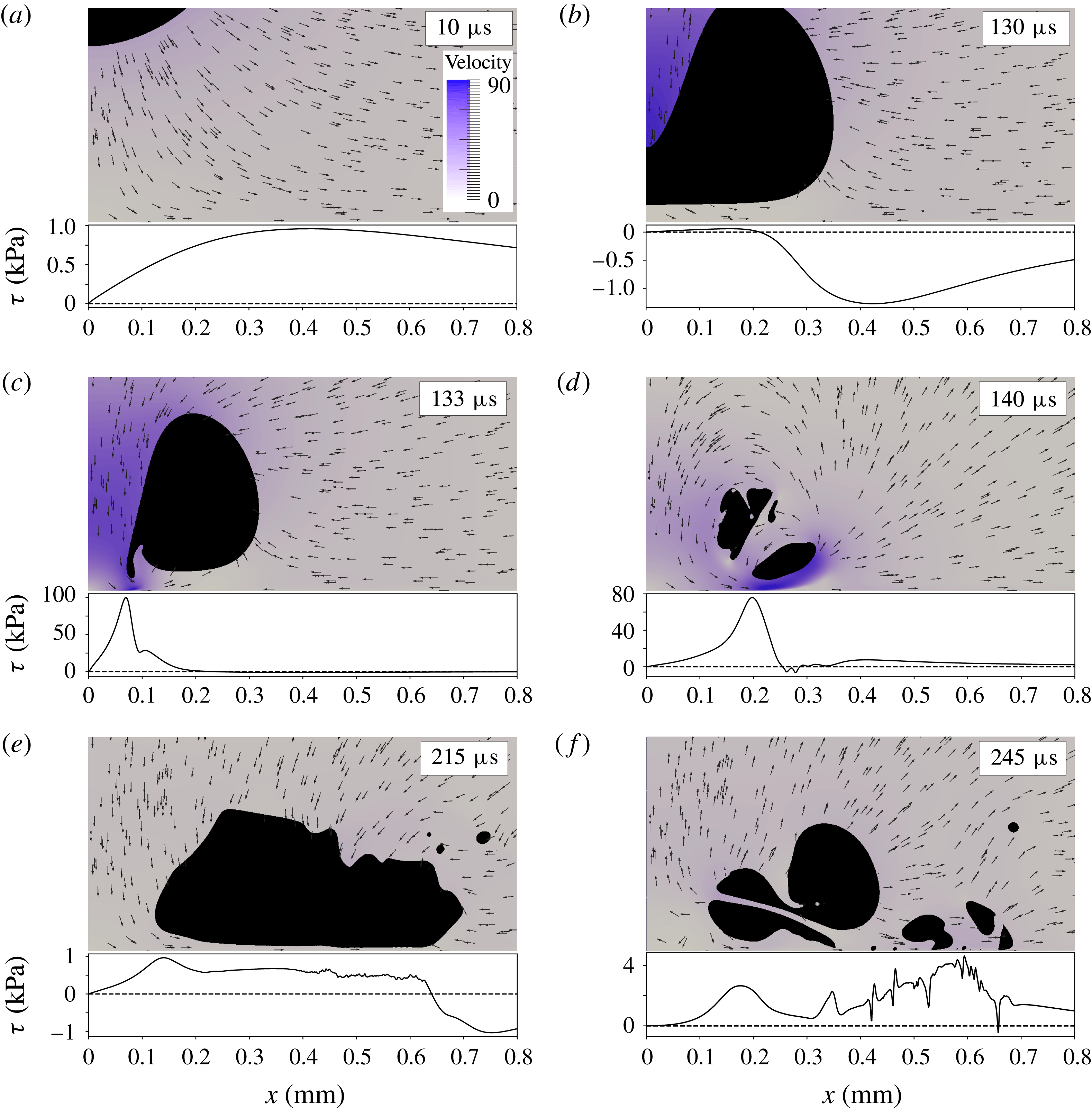
We now explore the flow within and near the gap formed between the bubble and the rigid boundary. Consecutive snapshots of six interesting points in time of the flow (
 $\unicode[STIX]{x1D6FE}=1.0$
,
 $R_{max}=0.6~\text{mm}$
) are shown in figure 5. The figure depicts the approach of the lower bubble wall towards the rigid boundary during the early bubble expansion (
 $t=10~\unicode[STIX]{x03BC}\text{s}$
), the early stage of jetting (
 $t=130~\unicode[STIX]{x03BC}\text{s}$
) and just after jet impact (
 $t=133~\unicode[STIX]{x03BC}\text{s}$
), then close to minimum volume (
 $t=140~\unicode[STIX]{x03BC}\text{s}$
) and during the torus collapse (
 $t=215~\unicode[STIX]{x03BC}\text{s}$
). The last frame in figure 5 shows the early third re-expansion (
 $t=245~\unicode[STIX]{x03BC}\text{s}$
). Below each frame in figure 5 the wall shear stress is plotted as a function of radial distance in units of
 $10^{3}~\text{Pa}$
. Please note that zero crossings of the wall shear stress are stagnation points (or rings). The magnitude of the velocity is colour coded. Owing to symmetry, the origin
 $x=0$
remains a stagnation point. At time
 $t=10~\unicode[STIX]{x03BC}\text{s}$
the wall shear stress follows the expected shape similar to a source position near an impermeable wall (Ye & Bull Reference Ye and Bull2006). During early collapse the interface closest to the wall flattens into an approximately
 $50~\unicode[STIX]{x03BC}\text{m}$
thin gap; see
 $t=130~\unicode[STIX]{x03BC}\text{s}$
. In this gap the shear stress increases with radial distance
 $x$
and reaches a mild maximum because the radial incoming flow decelerates this gap flow and reflects it upwards. A stagnation ring is created there that separates the positive and negative wall shear stresses. Up to this point in time, the magnitude of the wall shear stress is comparable with the ones during the spherical bubble expansion, i.e. around 1.0 kPa. A rapid increase of the wall shear stress is seen once the jet pierces, at approximately
 $80~\text{m}~\text{s}^{-1}$
, through the lower bubble wall and impacts on the boundary,
 $t=133~\unicode[STIX]{x03BC}\text{s}$
in figure 5. The shear stress increases from zero at the stagnation point to
 $\unicode[STIX]{x1D70F}\approx 100~\text{kPa}$
at the rim of the jet at
 $x=80~\unicode[STIX]{x03BC}\text{m}$
. Shortly afterwards, at
 $t=140~\unicode[STIX]{x03BC}\text{s}$
, the spreading jet flow dominates and creates a nearly purely outward-directed flow with positive wall shear stresses within the field of view. The maximum
 $\unicode[STIX]{x1D70F}$
has shifted downstream with a velocity of
 $19~\text{m}~\text{s}^{-1}$
. Away from the boundary, the jet flow is connected to the expanding flow, forming two anticlockwise-rotating vortex rings, a large-scale ring encompassing a smaller-scale vortex ring. The low pressure at their core stabilizes the expanding bubble fragments into an overall toroidal-shaped bubble. The last two frames in figure 5 depict the second collapse and re-expansion at
 $t=215~\unicode[STIX]{x03BC}\text{s}$
and
 $t=245~\unicode[STIX]{x03BC}\text{s}$
, respectively. During collapse we have a similar competition between the flow along the axis of symmetry (however, at a much lower velocity than the previous jet flow) with the inward flow due to the bubble acting as a sink. The stagnation ring is now located further away at
 $x\approx 640~\unicode[STIX]{x03BC}\text{m}$
at
 $t=215~\unicode[STIX]{x03BC}\text{s}$
. Yet the toroidal bubble fragments into many pieces, which leads to an even more complex flow pattern at
 $t=245~\unicode[STIX]{x03BC}\text{s}$
.
3.3 Spatio-temporal wall shear stress
The time–space map on the wall shear stress for a stand-off distance
 $\unicode[STIX]{x1D6FE}=1.0$
. The first colour bar represents the positive wall shear stress (away from the axis of symmetry), while the second one represents the negative wall shear stress. Overlaid is the bubble dynamics as a solid line and the instances shown in figure 5. The unit for
 $\unicode[STIX]{x1D70F}$
is Pa.

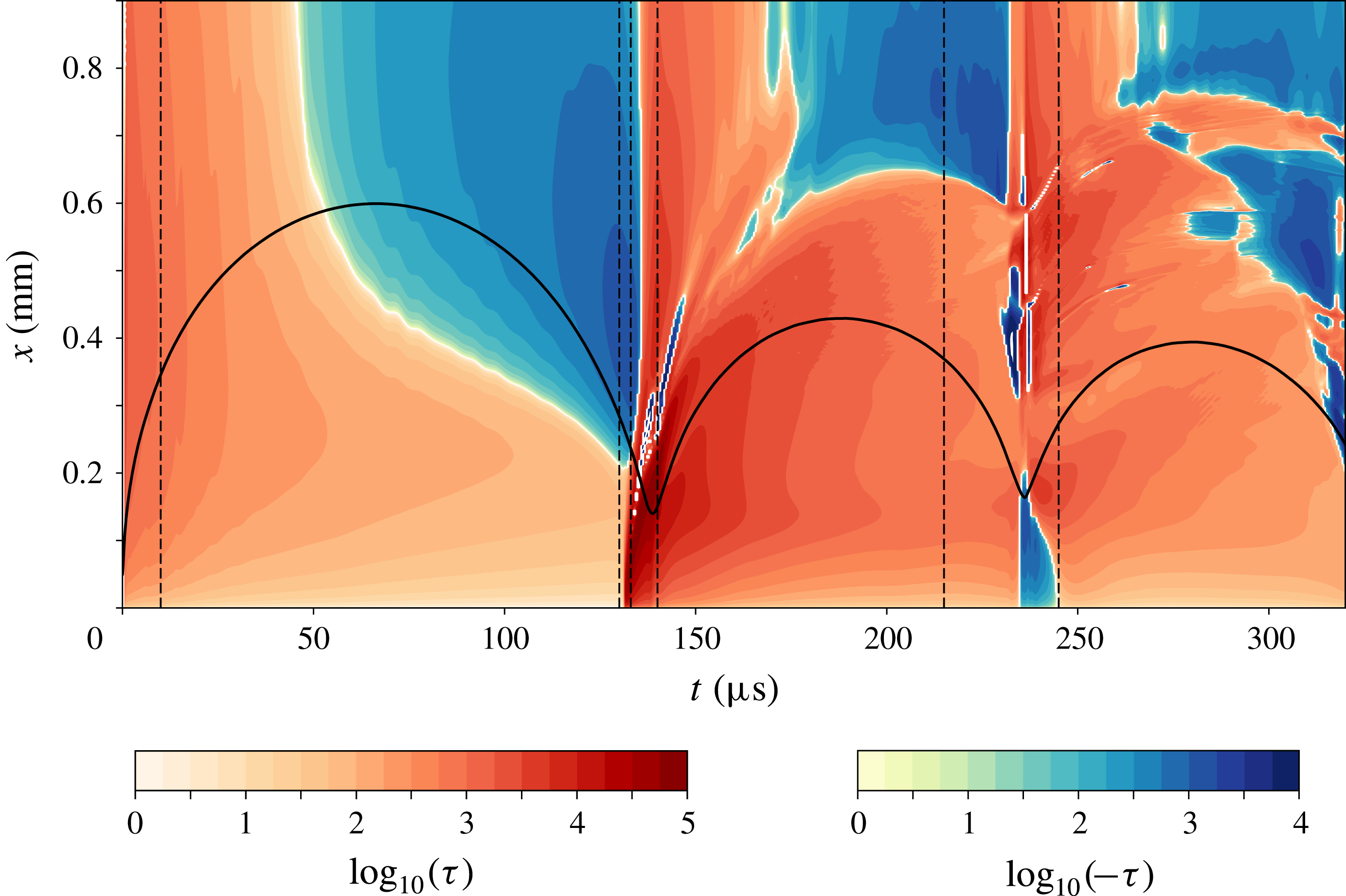
Figure 6 provides a detailed view on the spatio-temporal dynamics of the wall shear stress for
 $\unicode[STIX]{x1D6FE}=1.0$
. Positive values of the wall shear stress (directed away from the axis of symmetry) are plotted in red, while the stress towards
 $x=0$
is colour coded in blue. Because of the large range of values, the logarithm to the base 10 is taken of the wall shear stress values before plotting. It is evident that the highest stress occurs during the time of first minimum bubble volume
 $t\approx 135~\unicode[STIX]{x03BC}\text{s}$
near to the axis of symmetry
 $x\approx 0.15~\text{mm}$
. During most of the expansion (from
 $t=0~\unicode[STIX]{x03BC}\text{s}$
to
 $t\approx 50~\unicode[STIX]{x03BC}\text{s}$
) the stress is positive for the full domain, i.e. when the bubble expands rapidly. However, at a later stage of expansion (
 $t\approx 50~\unicode[STIX]{x03BC}\text{s}$
), the stress for large
 $x$
becomes negative because the expansion is slowed down and the upper bubble wall starts to move towards the boundary, driving the liquid at larger distances inwards. Near the axis of symmetry (
 $x<0.2~\text{mm}$
), the stresses decrease with time but remain positive for the whole expansion and collapse cycle. High stresses occur after
 $t\approx 132~\unicode[STIX]{x03BC}\text{s}$
in the small-
 $x$
region, which is the instant of time when the liquid jet impacts on the boundary and forms a boundary layer while spreading along the surface. The location of this outward-spreading flow is nicely captured in figure 6 by following the location of maximum stress as a function of time. Initially, the velocity is approximately
 $19~\text{m}~\text{s}^{-1}$
and drops to
 $1~\text{m}~\text{s}^{-1}$
at
 $t=200~\unicode[STIX]{x03BC}\text{s}$
. Moreover, negative stress is found ahead of the spreading flow (starts from
 $x\approx 170~\unicode[STIX]{x03BC}\text{m}$
at
 $t\approx 135~\unicode[STIX]{x03BC}\text{s}$
, moves to
 $x\approx 420~\unicode[STIX]{x03BC}\text{m}$
at
 $t\approx 146~\unicode[STIX]{x03BC}\text{s}$
), which is due to a reversed flow driven by a high adverse pressure gradient. This flow separation is detailed below in figure 7. The stress distribution during the re-expansion and later second collapse of the toroidal bubble differs greatly from the first oscillation cycle. Now a vortex ring has developed which continuously accelerates fluid anticlockwise, creating a positive shear stress for the entire second oscillation cycle (also see figure 5,
 $t=140~\unicode[STIX]{x03BC}\text{s}$
). During the second bubble collapse at time
 $t\approx 240~\unicode[STIX]{x03BC}\text{s}$
the wall shear stress distribution is more complex and the maximum of the shear stress occurs further away from the axis of symmetry (
 $x\approx 0.45~\text{mm}$
) due to the toroidal bubble collapse.
Flow separations during the jet spreading and bubble re-expansion. The radial velocity
 $U_{x}$
is colour coded, the blue colour indicating the reversed flow (flow to the axis of symmetry); the white lines represent the streamlines; the spatial units are
 $\unicode[STIX]{x03BC}\text{m}$
. Note that the offset of the
 $x$
-axis differs in the frames.

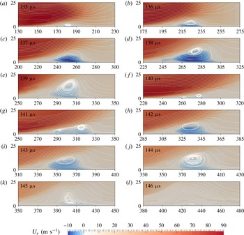
Figure 7 shows the boundary flow during the spreading of the impacting liquid jet, from
 $t=135~\unicode[STIX]{x03BC}\text{s}$
to
 $t=146~\unicode[STIX]{x03BC}\text{s}$
. Flow separations and the reversed flow are nicely captured by the streamline and the radial velocity contour. In figure 7, the radial velocity
 $U_{x}$
is colour coded: the red colour represents the flow directed away from the axis of symmetry, while blue colour indicates the reversed flow (flow to the axis of symmetry). The white lines are streamlines. At
 $t=135~\unicode[STIX]{x03BC}\text{s}$
, a vortex ring is nucleated at
 $x\approx 180~\unicode[STIX]{x03BC}\text{m}$
due to an adverse pressure caused by the fast flow spreading over the stagnant liquid. As a result, the flow close to the boundary is opposite to the main flow, resulting in a shear stress direction opposite to the driving jet flow. The vortex ring expands in size and moves outwards with a velocity of approximately
 $25~\text{m}~\text{s}^{-1}$
between
 $t=135~\unicode[STIX]{x03BC}\text{s}$
and
 $t=138~\unicode[STIX]{x03BC}\text{s}$
inducing a maximum negative velocity at
 $t=138~\unicode[STIX]{x03BC}\text{s}$
of
 $10~\text{m}~\text{s}^{-1}$
before it slows down at
 $t=139~\unicode[STIX]{x03BC}\text{s}$
. The flow from the re-expanding bubble triggers two new vortex rings at
 $t=141~\unicode[STIX]{x03BC}\text{s}$
which coalescence into a single ring at
 $t=142~\unicode[STIX]{x03BC}\text{s}$
and is transported with a velocity of approximately
 $20~\text{m}~\text{s}^{-1}$
before it decays at
 $t=146~\unicode[STIX]{x03BC}\text{s}$
.
4 Discussions and conclusion
The present simulations predict a complex spatio-temporal distribution of the wall shear stress during the non-spherical collapse of a bubble near a rigid wall. We have compared the temporal dynamics of the amplitude on the wall and found qualitative agreement with measurements. In particular, a short-lived stress of maximum amplitude is generated just after impact and during the early spreading of the jet, while a vortex ring that is formed during the re-expansion contributes for a longer-duration stress at a lower amplitude. The simulations predict stresses of the order of 50 kPa while the experimental results are an order of magnitude lower. The difference may be explained with the limited bandwidth and the calibrations conducted for the shear stress measurements. These were conducted over a range from 0.05 Pa to 10 Pa (Dijkink & Ohl Reference Dijkink and Ohl2008). Maisonhaute et al. (Reference Maisonhaute, Prado, White and Compton2002b
) provided a rough yet considerably higher estimate based on their earlier electrochemical measurements of the flow velocity of around
 $200~\text{m}~\text{s}^{-1}$
at the distance of 40–80 nm to the boundary (Maisonhaute, Brookes & Compton Reference Maisonhaute, Brookes and Compton2002a
). They predict that shear stress from oscillating and jetting bubbles driven by ultrasound could provide 25–50 bar. In contrast, bubbles oscillating only mildly with no or little deformation of their shape may create shear stresses of the order of a few kPa, according to simulations from Krasovitski & Kimmel (Reference Krasovitski and Kimmel2004).
Chahine et al. (Reference Chahine, Kapahi, Choi and Hsiao2016) have simulated the (inviscid) collapse of a bubble near a movable dirt particle with a focus on the forces generated by the pressure drag on the particle. Already, during expansion of the bubble, the particle may be pushed along the surface, while the complex recirculating flow after the bubble collapse may attract or push away the particle depending on the specific configuration. However, to understand the particle dynamics better, a more complex fluid–structure interaction model should be included.
The importance of the flow following the collapse of the bubble has also been acknowledged in the experimental study by Reuter & Mettin (Reference Reuter and Mettin2016). There the strongest cleaning effect was observed for
 $\unicode[STIX]{x1D6FE}\leqslant 1.1$
and was explained by the interaction of the jet spreading flow with the inward flow during the collapse. This results in a wall bound vortex creating a long-lasting exposure of the surface to shear. The present simulations confirm this scenario and are revealing the complex interaction leading to multiple stagnation rings and opposing directions of the shear stress.
Already during the expansion and early collapse of the bubble, the shear stresses are of the order of 1 kPa, while their increase to around 100 kPa occurs after the liquid jet impact. A system of vortex rings is formed under the combined effect of the main shear flow and the re-expansion of the toroidal bubble, which stabilizes the flow and thereby slows down the decay of the shear stress.
Starting from the present results, it will be interesting to conduct a detailed parameter study to evaluate the effect of bubble size, viscosity and density. For example, in ultrasound cleaning baths, smaller bubbles are found, which may not generate strong re-entrant jets (Kim & Kim Reference Kim and Kim2014) yet they translate along the surface (Kim et al. Reference Kim, Kim, Choi and Kim2009; Zijlstra et al. Reference Zijlstra, Janssens, Wostyn, Versluis, Mertens and Lohse2009). Simulations with suitable measurement techniques, which may still have to be developed, will help to understand how bubbles clean.
Acknowledgements
We acknowledge financial support from the Office of Naval Research under grant no. N62909-16-1-2139. We further thank Beng Hau Tan and the anonymous referees for their helpful suggestions to improve the manuscript.
Supplementary movie
A supplementary movie is available at https://doi.org/10.1017/jfm.2018.286.
Appendix A. Determination of the wall shear stress
To validate the calculation of wall shear stress from the code, we now reproduce the steady wall jet impingement simulation by Deshpande & Vaishnav (Reference Deshpande and Vaishnav1982): a cylindrical submerged jet impacting onto a no-slip flat surface. The jet has a radius of
 $R_{jet}=50~\unicode[STIX]{x03BC}\text{m}$
and a flat velocity of
 $U_{jet}$
, whose inlet is located
 $d=4R_{jet}=200~\unicode[STIX]{x03BC}\text{m}$
above the boundary. The domain is axisymmetric with both width and height of 10
 $R_{jet}$
. The mesh has a spacing
 $\unicode[STIX]{x0394}x=2.5~\unicode[STIX]{x03BC}\text{m}$
in the bulk flow while it is refined to
 $\unicode[STIX]{x0394}x=0.05~\unicode[STIX]{x03BC}\text{m}$
in the near-boundary region. Glauert (Reference Glauert1956) gave an analytic similarity solution of the wall shear stress for this problem:
 $$\begin{eqnarray}\displaystyle & \displaystyle \unicode[STIX]{x1D749}=\unicode[STIX]{x1D707}\!\left.{\displaystyle \frac{\text{d}\boldsymbol{u}_{\boldsymbol{r}}}{\text{d}y}}\right|_{y=0}=\unicode[STIX]{x1D70C}\left({\displaystyle \frac{125F^{3}\unicode[STIX]{x1D70C}}{216\unicode[STIX]{x1D707}x^{11}}}\right)^{1/4}, & \displaystyle\end{eqnarray}$$
where
 $\unicode[STIX]{x1D70C}$
is the flow density and
 $F$
is the momentum flux, which is defined as
 $F=(1/8)U_{jet}^{3}R_{jet}^{4}$
for a jet with a flat velocity profile.
Comparison of the wall shear stress of submerged jet impingement. (a) The normalized stress distribution on the wall for
 $Re=100$
; the blue line is the result of Deshpande & Vaishnav (Reference Deshpande and Vaishnav1982), the orange line and green dotted line represent the results calculated at
 $y=0.1~\unicode[STIX]{x03BC}\text{m}$
and
 $y=0.2~\unicode[STIX]{x03BC}\text{m}$
from the simulation, while the cyan dashed line is the Glauert solution. (b) The maximum normalized wall shear stress at various Reynolds numbers from Deshpande & Vaishnav (Reference Deshpande and Vaishnav1982) and the current simulations.

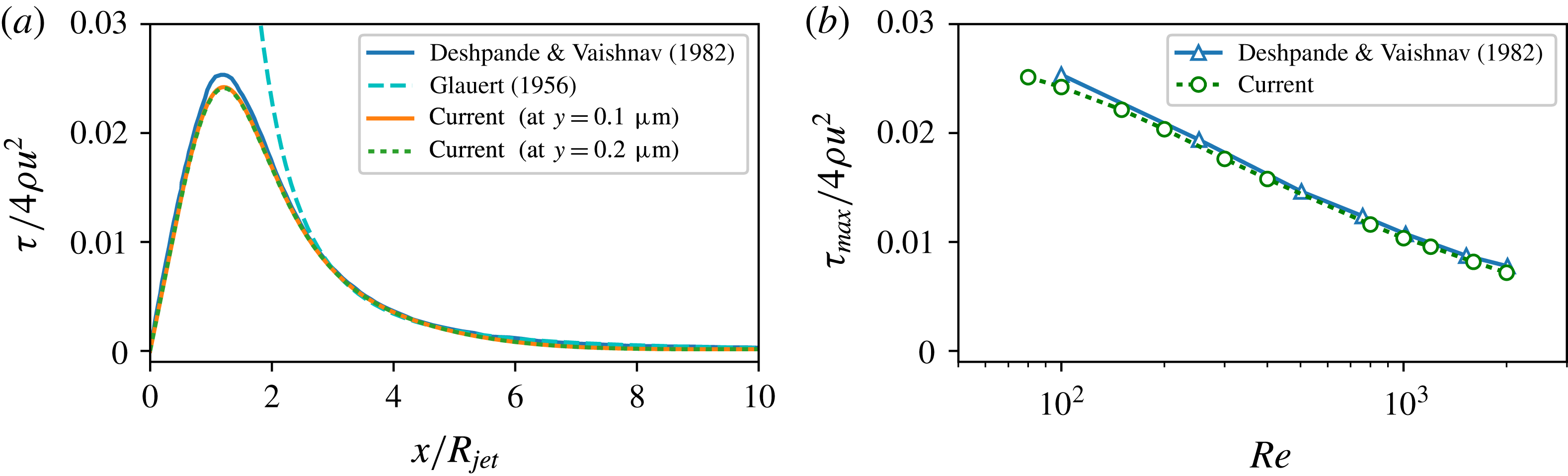
Figure 8(a) shows the comparison on the wall shear stress distribution along the boundary of our current calculation and the numerical result of Deshpande & Vaishnav (Reference Deshpande and Vaishnav1982) and the Glauert solution (A 1) for the case
 $Re=100$
, where
 $Re=2\unicode[STIX]{x1D70C}U_{jet}R_{jet}/\unicode[STIX]{x1D707}$
is the defined Reynolds number. The current calculations of the wall shear stress from (3.1) at
 $y=0.1~\unicode[STIX]{x03BC}\text{m}$
and
 $y=0.2~\unicode[STIX]{x03BC}\text{m}$
are indistinguishable, indicating that the stress is converged in the near-boundary cells and the flow field in the region with constant shear rate is resolved. The stress distribution along the boundary from the current simulation matches very well with Deshpande & Vaishnav (Reference Deshpande and Vaishnav1982) as well as the Glauert solution for
 $x/R_{jet}>3$
. The normalized maximum shear stress
 $\unicode[STIX]{x1D70F}_{max}/(4\unicode[STIX]{x1D70C}U_{jet}^{2})$
is also compared to the numerical work of Deshpande & Vaishnav (Reference Deshpande and Vaishnav1982, Reference Deshpande and Vaishnav1983), good agreement being found for a wide range of
 $Re$
numbers. Thus the calculation of the wall shear stress using our current model is reliable once the region with constant shear rate in the boundary layer is determined.