1 Introduction
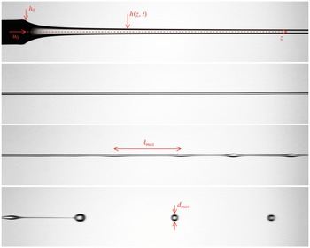
Seemingly simple questions are not always the simplest to answer quantitatively. A canonical illustration of this affirmation is the apparently simple problem of a liquid thread, falling from a nozzle by its own weight under the action of gravity, as shown in figure 1. As it falls, the thread eventually fragments into drops, a fact that we understand because locally it has a columnar shape, and thus suffers a capillary instability. However, how far from the nozzle exit does breakup happen? Even a distracted look at the possible scenarios lets one glimpse the potential difficulties of a precise analysis: a distance
 $z$
is the product of a velocity
 $u$
by a time
 $\unicode[STIX]{x1D70F}$
,
 $$\begin{eqnarray}z=u\unicode[STIX]{x1D70F}.\end{eqnarray}$$
Capillary breakup occurs within a time
 $\unicode[STIX]{x1D70F}$
which depends on the thread radius
 $h$
, the liquid density
 $\unicode[STIX]{x1D70C}$
, the viscosity
 $\unicode[STIX]{x1D702}$
and the surface tension
 $\unicode[STIX]{x1D6FE}$
, and we know that most of this time is spent in developing an instability about the quasicolumnar shape of the thread, the subsequent phenomena occurring around the pinching instant at the drop separation being comparatively much faster (Eggers & Villermaux Reference Eggers and Villermaux2008). The time
 $\unicode[STIX]{x1D70F}$
is either the capillary time
 $\sqrt{\unicode[STIX]{x1D70C}h^{3}/\unicode[STIX]{x1D6FE}}$
when inertia and surface tension are solely at play, or the viscous capillary time
 $\unicode[STIX]{x1D702}h/\unicode[STIX]{x1D6FE}$
if viscous effects dominantly slow down the unstable dynamics. When the jet issues from the nozzle ballistically, keeping its velocity and radius constant, the problem is indeed simple, and amounts to correct estimation of the relevant time scale
 $\unicode[STIX]{x1D70F}$
to compute the so-called ‘liquid intact length’ of the jet (see the corresponding section in Eggers & Villermaux (Reference Eggers and Villermaux2008) for a complete discussion and experimental references, including the case when the jet suffers a shear instability with the surrounding environment). Subtleties arise when the axial velocity of the jet depends on the axial distance
 $z$
.
Four successive panels showing a liquid jet (density
 $950~\text{kg}~\text{m}^{-3}$
, viscosity
 $\unicode[STIX]{x1D702}=50\times 10^{-3}$
Pa s) issuing from a round tube with radius
 $h_{0}=2$
mm at velocity
 $u_{0}=1~\text{cm}~\text{s}^{-1}$
, stretching in the gravity field (aligned with the
 $z$
direction), and thinning as it destabilizes through the growth of bulges separated by
 $\unicode[STIX]{x1D706}_{max}$
at breakup, producing stable drops of diameter
 $d_{max}$
.

A jet falling in the direction of gravity accelerates. If fed at a constant flow rate at the nozzle, stationarity implies that the thread radius thins with increasing distance from the exit. Therefore, if both
 $u$
and
 $h$
depend on the downstream distance, which estimates will correctly represent the breakup distance
 $z$
in (1.1): those at the nozzle exit, those at the breakup distance or a mixture of the two? As the radius thins, the instability may switch from an inertia dominated régime to a viscous dominated régime. Then, which time scale
 $\unicode[STIX]{x1D70F}$
should be considered to compute
 $z$
?
The detailed problem is even more subtle: the capillary instability preferentially amplifies a varicose perturbation, adjacent bulges along the thread feeding on the thinner ligament linking them (figure 1). The most amplified wavelength is proportional to
 $h$
, the other wavelengths having a weaker growth rate. Since the jet accelerates, mass conservation of the incompressible liquid also implies that the distance between two adjacent instability crests increases with larger distances from the nozzle exit. The capillary instability has thus to compete with another phenomenon, namely jet stretching, characterized by another time scale
 $(\unicode[STIX]{x2202}_{z}u)^{-1}$
. There are thus three time scales that may potentially contribute to
 $\unicode[STIX]{x1D70F}$
, which all depend intrinsically on the distance from the nozzle. Deciding a priori which one will dominate and how is a hazardous exercise.
Deciphering of the relative importance of the coupled effects mentioned above requires an instability analysis accounting for both the substrate deformation (jet stretching) and the modification of the local instability dispersion relation as the jet thins (to describe the growing relative influence of viscosity). This question has been envisaged in the very viscous limit by Tomotika (Reference Tomotika1936), for the particular case where
 $u$
increases linearly with
 $z$
by Frankel & Weihs (Reference Frankel and Weihs1985, Reference Frankel and Weihs1987) and more recently by Sauter & Buggisch (Reference Sauter and Buggisch2005), Senchenko & Bohr (Reference Senchenko and Bohr2005) and Javadi et al. (Reference Javadi, Eggers, Bonn, Habibi and Ribe2013) for a gravitationally accelerated jet.
These last authors quantified the maximum gain that perturbations can reach at a given location using a local plane wave decomposition (WKBJ approximation). By choosing adequately the gain needed for breakup, they were able to collapse measurements of the breakup distance on a theoretical curve. They also obtained an asymptotic expression in the viscous régime consistent with the anticipated scaling law, which compares the viscous capillary time scale based on the current jet radius with the stretching time of the jet.
In the present work, we use a similar approach to that of Javadi et al. (Reference Javadi, Eggers, Bonn, Habibi and Ribe2013) by searching for maximum perturbation gains using WKBJ approximations. In addition to providing much more detail, we extend their analysis in several ways. We first consider all of the régimes ranging from very viscous to inviscid. We then compare the maximum gain and the most dangerous frequency of the perturbations for two types of excitation: (1) nozzle excitation (the perturbation is introduced at the nozzle only) and (2) background noise (the perturbation is present everywhere). We finally provide predictions for the breakup wavelength and the resulting droplet size.
The paper is organized as follows. In § 2, we present the mathematical formulation by providing the model for the base flow and the perturbations. An expression of the perturbation gain is derived using the WKBJ framework. In § 3, the result of the optimization procedure maximizing the gain is provided for each type of excitation. The breakup distance, the most dangerous frequency, the wavelength and the droplet size are analysed as functions of the gain and fluid viscosity (Ohnesorge number
 $\mathit{Oh}$
). Asymptotic formulae for weak and strong viscosity (small and large
 $\mathit{Oh}$
) are provided in this section, though their derivation is given in an appendix at the end of the paper. For nozzle excitation, a peculiar behaviour of the optimal perturbation observed for intermediate Ohnesorge numbers (
 $0.1<\mathit{Oh}<1$
) is further discussed in § 4. We show that the peak of the breakup wavelength obtained for
 $\mathit{Oh}\approx 0.3$
is related to a property of the local dispersion relation outside the instability band. The results are compared with local predictions in § 5 and applied to realistic configurations in § 6.
2 Mathematical formulation
We consider an axisymmetric liquid jet falling vertically by the action of gravity
 $g$
. The jet has a radius
 $h_{0}$
and a characteristic velocity
 $u_{0}$
at the nozzle (figure 1). The fluid has a density
 $\unicode[STIX]{x1D70C}$
, a viscosity
 $\unicode[STIX]{x1D708}=\unicode[STIX]{x1D702}/\unicode[STIX]{x1D70C}$
and a surface tension
 $\unicode[STIX]{x1D6FE}$
. The surrounding environment is considered as evanescent, and is neglected.
2.1 Base flow
Spatial and time variables are non-dimensionalized using the radius
 $h_{0}$
and the capillary time
 $\unicode[STIX]{x1D70F}_{c}=\sqrt{\unicode[STIX]{x1D70C}h_{0}^{3}/\unicode[STIX]{x1D6FE}}$
respectively. The base flow is governed by three parameters:
 $$\begin{eqnarray}\displaystyle & \displaystyle Q=u_{0}\sqrt{\frac{\unicode[STIX]{x1D70C}h_{0}}{\unicode[STIX]{x1D6FE}}},\quad \text{the flow rate}, & \displaystyle\end{eqnarray}$$
 $$\begin{eqnarray}\displaystyle & \displaystyle \mathit{Oh}=\unicode[STIX]{x1D708}\sqrt{\frac{\unicode[STIX]{x1D70C}}{\unicode[STIX]{x1D6FE}h_{0}}},\quad \text{the Ohnesorge number}, & \displaystyle\end{eqnarray}$$
 $$\begin{eqnarray}\displaystyle & \displaystyle \mathit{Bo}=\frac{\unicode[STIX]{x1D70C}gh_{0}^{2}}{\unicode[STIX]{x1D6FE}}\quad \text{the Bond number}. & \displaystyle\end{eqnarray}$$
 $\mathit{We}=Q^{2}$
instead of the dimensionless flow rate. The Ohnesorge number is the ratio of the viscous capillary time scale to the capillary time scale. We describe the liquid jet by the one-dimensional model (Trouton Reference Trouton1906; Weber Reference Weber1931; Eggers & Villermaux Reference Eggers and Villermaux2008)
 $$\begin{eqnarray}\displaystyle & \displaystyle \frac{\unicode[STIX]{x2202}A}{\unicode[STIX]{x2202}t}+\frac{\unicode[STIX]{x2202}(Au)}{\unicode[STIX]{x2202}z}=0, & \displaystyle\end{eqnarray}$$
 $$\begin{eqnarray}\displaystyle & \displaystyle \frac{\unicode[STIX]{x2202}u}{\unicode[STIX]{x2202}t}+u\frac{\unicode[STIX]{x2202}u}{\unicode[STIX]{x2202}z}=3\mathit{Oh}\frac{1}{A}\frac{\unicode[STIX]{x2202}}{\unicode[STIX]{x2202}z}\left(A\frac{\unicode[STIX]{x2202}u}{\unicode[STIX]{x2202}z}\right)+\frac{\unicode[STIX]{x2202}K}{\unicode[STIX]{x2202}z}+\mathit{Bo}, & \displaystyle\end{eqnarray}$$
 $$\begin{eqnarray}K=\frac{4AA_{zz}-2A_{z}^{2}}{[4A+A_{z}^{2}]^{3/2}}-\frac{2}{[4A+A_{z}^{2}]^{1/2}},\end{eqnarray}$$
where
 $u(z,t)$
is the local axial velocity,
 $A=h^{2}$
is the square of the local radius
 $h(z,t)$
,
 $z$
is the axial coordinate oriented downward,
 $t$
is the time variable, and
 $A_{z}$
and
 $A_{zz}$
are respectively the first and second derivatives of
 $A$
with respect to
 $z$
. The boundary conditions at the nozzle are
 $$\begin{eqnarray}A(z=0,t)=1,\quad u(z=0,t)=Q.\end{eqnarray}$$
The stationary base flow satisfies
 $$\begin{eqnarray}\displaystyle & \displaystyle \frac{\unicode[STIX]{x2202}(A_{0}U_{0})}{\unicode[STIX]{x2202}z}=0, & \displaystyle\end{eqnarray}$$
 $$\begin{eqnarray}\displaystyle & \displaystyle U_{0}\frac{\unicode[STIX]{x2202}U_{0}}{\unicode[STIX]{x2202}z}=3\mathit{Oh}\frac{1}{A_{0}}\frac{\unicode[STIX]{x2202}}{\unicode[STIX]{x2202}z}\left(A_{0}\frac{\unicode[STIX]{x2202}U_{0}}{\unicode[STIX]{x2202}z}\right)+\frac{\unicode[STIX]{x2202}K_{0}}{\unicode[STIX]{x2202}z}+\mathit{Bo}. & \displaystyle\end{eqnarray}$$
 $$\begin{eqnarray}A_{0}U_{0}=Q.\end{eqnarray}$$
We will consider the régime where the jet base flow is inertial and is given at leading order by
 $$\begin{eqnarray}U_{0}\frac{\unicode[STIX]{x2202}U_{0}}{\unicode[STIX]{x2202}z}=\mathit{Bo}.\end{eqnarray}$$
This hypothesis amounts to neglecting viscous and curvature effects in the jet evolution. Because it accelerates as it falls, the jet gets thinner and slenderer. Curvature effects along
 $z$
thus soon vanish (unless the jet is initially very small, see Rubio-Rubio, Sevilla & Gordillo Reference Rubio-Rubio, Sevilla and Gordillo2013), and viscous stresses applying on the jet cross-section are also soon overcome by the gravity force (beyond a physical distance from the nozzle of order
 $\sqrt{\unicode[STIX]{x1D708}u_{0}/g}$
, see Clarke Reference Clarke1969). Equations (2.6) and (2.7) thus give
 $$\begin{eqnarray}\displaystyle & \displaystyle U_{0}(z)=\sqrt{2\mathit{Bo }z+Q^{2}}, & \displaystyle\end{eqnarray}$$
 $$\begin{eqnarray}\displaystyle & \displaystyle A_{0}(z)=\frac{Q}{\sqrt{2\mathit{Bo }z+Q^{2}}}. & \displaystyle\end{eqnarray}$$
 $z$
. Viscous and curvature terms are therefore negligible along the entire jet, if they are already negligible in the vicinity of the nozzle exit. This is satisfied if the flow rate is sufficiently large, and more precisely if the following conditions are met:
 $$\begin{eqnarray}\displaystyle & \displaystyle Q\gg 1, & \displaystyle\end{eqnarray}$$
 $$\begin{eqnarray}\displaystyle & \displaystyle Q^{2}\gg \mathit{Bo}, & \displaystyle\end{eqnarray}$$
 $$\begin{eqnarray}\displaystyle & \displaystyle Q^{3}\gg \mathit{Bo}\mathit{Oh}. & \displaystyle\end{eqnarray}$$
 $Q$
,
 $\mathit{Bo}$
and
 $\mathit{Oh}$
are defined from the local values of
 $U_{0}$
and
 $A_{0}$
, conditions (2.9a
)–(2.9c
) are always satisfied sufficiently far away from the nozzle (e.g. Sauter & Buggisch Reference Sauter and Buggisch2005). Since the phenomena we will describe result from a dynamics that integrates over distances much larger than the jet initial radius, we use here (2.8b
) as a good approximation of the base flow everywhere.
For simplicity, we assume in the following that
 $Q$
is the only large parameter,
 $\mathit{Bo}$
and
 $\mathit{Oh}$
being of order 1 or smaller. Both
 $U_{0}$
and
 $A_{0}$
then vary with respect to the slow variable
 $$\begin{eqnarray}Z=\frac{z}{z_{o}}+1\end{eqnarray}$$
as
 $$\begin{eqnarray}\displaystyle & \displaystyle U_{0}(Z)=Q\sqrt{Z}, & \displaystyle\end{eqnarray}$$
 $$\begin{eqnarray}\displaystyle & \displaystyle A_{0}(Z)=1/\sqrt{Z}, & \displaystyle\end{eqnarray}$$
 $$\begin{eqnarray}z_{o}=\frac{Q^{2}}{2\mathit{Bo}}\end{eqnarray}$$
is the (large) non-dimensionalized variation scale of the base flow.
2.2 Perturbations
We now consider linear perturbations
 $(u_{p},A_{p})$
in velocity and cross-section to the above base flow. These perturbations satisfy the linear system
 $$\begin{eqnarray}\displaystyle & \displaystyle \displaystyle \frac{\unicode[STIX]{x2202}A_{p}}{\unicode[STIX]{x2202}t}=-\displaystyle \frac{\unicode[STIX]{x2202}(A_{p}U_{0}+A_{0}u_{p})}{\unicode[STIX]{x2202}z}, & \displaystyle\end{eqnarray}$$
 $$\begin{eqnarray}\displaystyle & \displaystyle \displaystyle \frac{\unicode[STIX]{x2202}u_{p}}{\unicode[STIX]{x2202}t}+\displaystyle \frac{\unicode[STIX]{x2202}u_{p}U_{0}}{\unicode[STIX]{x2202}z}=3\frac{\mathit{Oh}}{A_{0}}\left\{\frac{\unicode[STIX]{x2202}}{\unicode[STIX]{x2202}z}\left(A_{0}\frac{\unicode[STIX]{x2202}u_{p}}{\unicode[STIX]{x2202}z}+A_{p}\displaystyle \frac{\unicode[STIX]{x2202}U_{0}}{\unicode[STIX]{x2202}z}\right)-\frac{A_{p}}{A_{0}}\displaystyle \frac{\unicode[STIX]{x2202}}{\unicode[STIX]{x2202}z}\left(A_{0}\displaystyle \frac{\unicode[STIX]{x2202}U_{0}}{\unicode[STIX]{x2202}z}\right)\right\}+\frac{\unicode[STIX]{x2202}{\mathcal{L}}(A_{p})}{\unicode[STIX]{x2202}z}, & \displaystyle \nonumber\\ \displaystyle & & \displaystyle\end{eqnarray}$$
 ${\mathcal{L}}(A_{p})$
is the linear operator obtained by linearizing
 $K-K_{0}$
around
 $A_{0}$
.
We want to analyse these perturbations in the ‘jetting’ régime when the jet is globally stable. More precisely, we do not consider the global transition that leads to dripping and which has been studied elsewhere (Le Dizès Reference Le Dizès1997; Sauter & Buggisch Reference Sauter and Buggisch2005; Rubio-Rubio et al.
Reference Rubio-Rubio, Sevilla and Gordillo2013). We are interested in the growth of the perturbations that give rise to the formation of droplets far away from the nozzle. In this régime, the jet is convectively unstable: the perturbations are advected downstream as they grow. We expect droplets to form when the perturbation has reached a sufficiently large amplitude. Of particular interest is the maximum amplitude that perturbations can reach at a given location
 $z_{f}$
from a fixed level of noise. This amounts to calculating the maximum spatial gain that perturbations can exhibit at a given downstream location. For this purpose, we will consider two situations.
-
(i) Fluctuations are mainly present at the nozzle, as in laboratory experiments where the jet nozzle is vibrated, for instance (Sauter & Buggisch Reference Sauter and Buggisch2005). In this case, we are interested in the spatial gain at
 $z_{f}$
of perturbations generated at the nozzle,
$z=0$
.
-
(ii) The jet is subject to a background noise which acts at every
$z$
location. In this case, we are interested in the maximum gain at
$z_{f}$
of perturbations that originate from anywhere along the jet. In other words, we are interested in the spatial gain between
$z_{i}$
and
$z_{f}$
, where
$z_{i}$
is chosen such that the gain is maximum. Obviously, the gain in this case is larger than in (i), since
$z=0$
is one particular excitation location among the many possible in this case.


The base flow is stationary; a temporal excitation at a given location with a fixed frequency leads to a temporal response in the whole jet with the same frequency. As the jet can be forced on
 $A$
or on
 $u$
, we expect two independent spatial structures associated with each frequency. If we write
 $$\begin{eqnarray}(u_{p},A_{p})=(\tilde{u} ,\tilde{A})\text{e}^{-\text{i}\unicode[STIX]{x1D714}t}+\text{c.c.},\end{eqnarray}$$
the normalized solution forced in
 $u$
at the nozzle will satisfy
 $\tilde{A}(z=0)=0$
,
 $\tilde{u} (z=0)=1$
, while the one forced in
 $A$
at the nozzle will satisfy
 $\tilde{A}(z=0)=1$
,
 $\tilde{u} (z=0)=0$
. A linear combination of these two solutions can be used to obtain the normalized solution forced in
 $u$
or forced in
 $A$
at any location
 $z_{i}$
.
We then define a spatial gain in
 $A$
from
 $z_{i}$
to
 $z_{f}$
from the solution forced in
 $A$
at
 $z_{i}$
by
 $G_{A}(z_{i},z_{f})=|\tilde{A}(z_{f})|$
. Similarly, we define a spatial gain in
 $u$
from
 $z_{i}$
to
 $z_{f}$
from the solution forced in
 $u$
at
 $z_{i}$
by
 $G_{u}(z_{i},z_{f})=|\tilde{u} (z_{f})|$
.
Both
 $U_{0}$
and
 $A_{0}$
depend on the slow spatial variable
 $Z$
. Anticipating that the typical wavelength will be of order 1, a local plane wave approximation (WKBJ approximation) can be used (Bender & Orszag Reference Bender and Orszag1978). In other words, each time-harmonic perturbation amplitude can be written as a sum of expressions of the form (WKBJ approximation)
 $$\begin{eqnarray}(\tilde{u} ,\tilde{A})=(v(Z),a(Z))\text{e}^{\text{i}z_{o}\int ^{Z}k(s)\,\text{d}s},\end{eqnarray}$$
where
 $k(Z)$
,
 $v(Z)$
and
 $a(Z)$
depend on the slow variation scale of the base flow. With the WKBJ ansatz, the perturbation equations become at leading order in
 $1/z_{o}$
 $$\begin{eqnarray}\displaystyle & \displaystyle (-\text{i}\unicode[STIX]{x1D714}+\text{i}kU_{0})a+\text{i}kA_{0}v=0, & \displaystyle\end{eqnarray}$$
 $$\begin{eqnarray}\displaystyle & \displaystyle (-\text{i}\unicode[STIX]{x1D714}+\text{i}kU_{0})v=-3\mathit{Oh}k^{2}v+\frac{\text{i}k}{2A_{0}^{3/2}}(1-k^{2}A_{0})a. & \displaystyle\end{eqnarray}$$
 $$\begin{eqnarray}(-\text{i}\unicode[STIX]{x1D714}+\text{i}kU_{0})^{2}+3\mathit{Oh}k^{2}(-\text{i}\unicode[STIX]{x1D714}+\text{i}kU_{0})-\frac{k^{2}}{2\sqrt{A_{0}}}(1-k^{2}A_{0})=0.\end{eqnarray}$$
This equation provides
 $k$
as a function of
 $Z$
. Expressions for
 $v(Z)$
and
 $a(Z)$
can be obtained by considering the problem to the next order (see appendix B).
Among the four possible solutions to (2.17), only the two wavenumbers corresponding to waves propagating downstream are allowed. As explained in Bers (Reference Bers1983) (see also Huerre & Monkewitz Reference Huerre and Monkewitz1990), these wavenumbers are the analytic continuations for real
 $\unicode[STIX]{x1D714}$
of functions satisfying
 $\text{Im}(k)>0$
for large
 $\text{Im}(\unicode[STIX]{x1D714})$
. They are well defined in the convective régime that we consider here.
If
 $\unicode[STIX]{x1D714}=\overline{\unicode[STIX]{x1D714}}Q$
with
 $\overline{\unicode[STIX]{x1D714}}=O(1)$
, the wavenumbers associated with the downstream propagating waves can be expanded as
 $$\begin{eqnarray}k\sim k_{0}+\frac{k_{1}}{Q},\end{eqnarray}$$
where
 $k_{0}$
is found to be identical for both waves:
 $$\begin{eqnarray}k_{0}=\frac{\unicode[STIX]{x1D714}}{U_{0}}=\overline{\unicode[STIX]{x1D714}}A_{0}.\end{eqnarray}$$
At the order
 $1/Q$
, we get
 $$\begin{eqnarray}k_{1}=-\text{i}\left\{\frac{k_{0}A_{0}^{3/4}}{\sqrt{2}}\sqrt{1-A_{0}k_{0}^{2}+\frac{9\mathit{Oh }^{2}\sqrt{A_{0}}k_{0}^{2}}{2}}-\frac{3\mathit{Oh}k_{0}^{2}A_{0}}{2}\right\}.\end{eqnarray}$$
The two wavenumbers are obtained by considering the two possible values of the square root. Although both waves are needed to satisfy the boundary conditions at the nozzle, the solution is rapidly dominated downstream by a single wave corresponding to the wavenumber with the smallest imaginary part.
Both the solution forced in
 $A$
and the solution forced in
 $u$
are thus expected to have a similar WKBJ approximation (2.15). The main contribution to the two gains
 $G_{A}(z_{i},z_{f})$
and
 $G_{u}(z_{i},z_{f})$
is therefore expected to be the same and to be given by the exponential factor
 $$\begin{eqnarray}G(z_{i},z_{f})=\text{e}^{S(Z_{i},Z_{f})},\end{eqnarray}$$
where
 $$\begin{eqnarray}S(Z_{i},Z_{f})=-z_{o}\int _{Z_{i}}^{Z_{f}}\text{Im}(k)(Z)\,\text{d}Z=-\frac{z_{o}}{Q}\int _{Z_{i}}^{Z_{f}}\text{Im}(k_{1})(Z)\,\text{d}Z.\end{eqnarray}$$
This implicitly assumes that
 $z_{o}/Q=Q/2\mathit{Bo}$
is large. When
 $z_{o}/Q=O(1)$
, the WKBJ approach remains valid but the gain (2.21) is of the same order of magnitude as the variation of
 $v$
and
 $a$
. In this case, one should a priori take into account the amplitudes
 $v$
and
 $a$
provided in appendix B and apply the boundary conditions explicitly at the forcing location. This leads to different gains for a forcing in velocity and a forcing in radius.
The gain
 $G$
is associated with the temporal growth of the local perturbation. Indeed,
 $S$
can be written as
 $$\begin{eqnarray}S=z_{o}\int _{Z_{i}}^{Z_{f}}\frac{\unicode[STIX]{x1D70E}(k_{l}(Z),\mathit{Oh}_{l}(Z))}{\unicode[STIX]{x1D70F}_{c_{l}}(Z)U_{0}(Z)}\,\text{d}Z,\end{eqnarray}$$
where
 $\unicode[STIX]{x1D70E}(k,\mathit{Oh})$
is the growth rate of the capillary instability for the 1D model:
 $$\begin{eqnarray}\unicode[STIX]{x1D70E}(k,\mathit{Oh})=\frac{k}{\sqrt{2}}\sqrt{1-k^{2}+\frac{9\mathit{Oh }^{2}k^{2}}{2}}-\frac{3\mathit{Oh}k^{2}}{2}.\end{eqnarray}$$
The local wavenumber
 $k_{l}(Z)$
, local Ohnesorge number
 $\mathit{Oh}_{l}(Z)$
and local capillary time scale
 $\unicode[STIX]{x1D70F}_{c_{l}}(Z)$
vary as
 $$\begin{eqnarray}\displaystyle & \displaystyle k_{l}(Z)=\overline{\unicode[STIX]{x1D714}}Z^{-3/8}, & \displaystyle\end{eqnarray}$$
 $$\begin{eqnarray}\displaystyle & \displaystyle \mathit{Oh}_{l}(Z)=\mathit{Oh}Z^{1/8}, & \displaystyle\end{eqnarray}$$
 $$\begin{eqnarray}\displaystyle & \displaystyle \unicode[STIX]{x1D70F}_{c_{l}}(Z)=Z^{-3/8}. & \displaystyle\end{eqnarray}$$
In the following, we write
 $S$
as
 $$\begin{eqnarray}S=\frac{z_{o}}{\sqrt{2}Q}\overline{S}(Z_{f},Z_{i},\mathit{Oh},\overline{\unicode[STIX]{x1D714}}),\end{eqnarray}$$
with
 $$\begin{eqnarray}\overline{S}(Z_{i},Z_{f},\overline{\unicode[STIX]{x1D714}},\mathit{Oh})=\overline{\unicode[STIX]{x1D714}}\int _{Z_{i}}^{Z_{f}}z^{-7/8}\left(\sqrt{1-\overline{\unicode[STIX]{x1D714}}^{2}z^{-3/2}+\frac{9\mathit{Oh }^{2}\overline{\unicode[STIX]{x1D714}}^{2}}{2}z^{-5/4}}-\frac{3\mathit{Oh}\overline{\unicode[STIX]{x1D714}}}{\sqrt{2}}z^{-5/8}\right)\text{d}z.\end{eqnarray}$$
Our objective is to find the frequency
 $\overline{\unicode[STIX]{x1D714}}$
that gives the largest value of
 $\overline{S}$
at a given
 $Z_{f}$
. For the type of perturbations in case (i) (nozzle excitation),
 $Z_{i}=1$
, and we are looking for
 $$\begin{eqnarray}\overline{S}_{max}^{(a)}(Z_{f},\mathit{Oh})=\max _{\overline{\unicode[STIX]{x1D714}}}\overline{S}(1,Z_{f},\overline{\unicode[STIX]{x1D714}},\mathit{Oh}).\end{eqnarray}$$
For the type of perturbations in case (ii) (background noise), the gain is maximized over all
 $Z_{i}$
between 1 and
 $Z_{f}$
, so
 $$\begin{eqnarray}\overline{S}_{max}^{(b)}(Z_{f},\mathit{Oh})=\max _{\overline{\unicode[STIX]{x1D714}}}\max _{1\leqslant Z_{i}<Z_{f}}\overline{S}(Z_{i},Z_{f},\overline{\unicode[STIX]{x1D714}},\mathit{Oh}).\end{eqnarray}$$
For
 $z>1$
, the integrand in the expression of
 $\overline{S}$
is always positive when
 $\overline{\unicode[STIX]{x1D714}}<1$
. This means that as long as
 $\overline{\unicode[STIX]{x1D714}}_{max}^{(a)}\leqslant 1$
, the gain cannot be increased by changing
 $Z_{i}$
, and we have
 $\overline{S}_{max}^{(b)}=\overline{S}_{max}^{(a)}$
. When
 $\overline{\unicode[STIX]{x1D714}}_{max}^{(a)}>1$
, the perturbation starts to decrease before increasing further downstream. In this case, the gain can be increased by considering larger
 $Z_{i}$
. More precisely,
 $Z_{i}$
has to be chosen such that the integrand starts to be positive, which gives
 $Z_{i}=\overline{\unicode[STIX]{x1D714}}^{4/3}$
. In this régime,
 $$\begin{eqnarray}\overline{S}_{max}^{(b)}(Z_{f},\mathit{Oh})=\max _{\overline{\unicode[STIX]{x1D714}}}\overline{S}(\overline{\unicode[STIX]{x1D714}}^{4/3},Z_{f},\overline{\unicode[STIX]{x1D714}},\mathit{Oh}).\end{eqnarray}$$
Both
 $\overline{S}_{max}^{(a)}$
and
 $\overline{S}_{max}^{(b)}$
are obtained using standard Matlab subroutines.
3 Quantitative results
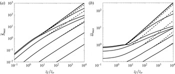
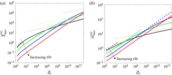
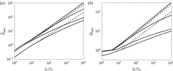
The results of the optimization procedure are shown in figure 2 for both nozzle excitation and background noise. Both the maximum gain and the most dangerous frequency are plotted versus the rescaled distance
 $z_{f}/z_{o}$
from the nozzle for
 $\mathit{Oh}$
ranging from
 $10^{-4}$
to
 $10^{3}$
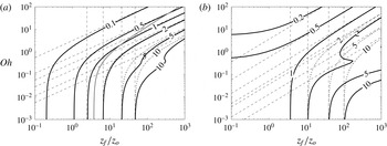
. The same results are shown as level curves in the
 $(z_{f}/z_{o},\mathit{Oh})$
plane in figure 3. As expected,
 $\overline{S}_{max}$
grows as
 $z_{f}/z_{o}$
increases or
 $\mathit{Oh}$
decreases (see figure 2
a). The most dangerous frequency follows the same trend (see figure 2
b). As already mentioned above, nozzle excitation (case (i)) and background noise (case (ii)) provide the same results when
 $\overline{\unicode[STIX]{x1D714}}_{max}\leqslant 1$
. The contour
 $\overline{\unicode[STIX]{x1D714}}_{max}=1$
has been reported in figure 3(a) as a dotted line. On the left of this dotted line, the contours of maximum gain are then the same for both cases. When
 $\overline{\unicode[STIX]{x1D714}}_{max}$
is larger than 1, background noise gain becomes larger than nozzle excitation gain. The most dangerous frequency for background noise also becomes larger than that for nozzle excitation. It should be noted, however, that significant differences are only observed in an intermediate régime of
 $\mathit{Oh}$
(typically
 $10^{-2}<\mathit{Oh}<1$
) for large values of
 $\overline{S}$
(
 $\overline{S}>5$
) (see figure 3).
Maximum gain
 $\overline{S}_{max}$
(a) and most dangerous frequency
 $\overline{\unicode[STIX]{x1D714}}_{max}$
(b) of the perturbations excited from background noise (dashed lines) and at the nozzle (solid lines) as a function of the distance
 $z_{f}/z_{o}=Z_{f}-1$
from the nozzle. From bottom to top,
 $\mathit{Oh}$
takes the values 1000, 100, 10, 1, 0.1, 0.01 and
 $10^{-4}$
.

Level curves of the maximum gain
 $\overline{S}_{max}$
(a) and the most dangerous frequency
 $\overline{\unicode[STIX]{x1D714}}_{max}$
(b) of the perturbations excited from background noise (dashed lines) and at the nozzle (solid lines) in the
 $(z_{f}/z_{o},\mathit{Oh})$
plane. The dashed lines correspond to the asymptotic limits (3.11) and (3.5) for small and large
 $\mathit{Oh}$
respectively. On the left of the
 $\unicode[STIX]{x1D714}_{max}=1$
curve (indicated as a grey line in (a)), the solid and dashed lines are superimposed.

Figure 3 can be used to obtain the distance of the expected transition to jet breakup and droplet formation. We assume that a gain of order
 $G_{t}\approx \text{e}^{7}$
, that is
 $S_{t}=7$
, is enough for the transition, a value commonly admitted in boundary layer instabilities (Schlichting Reference Schlichting1987). From (2.26), we can deduce the value of
 $\overline{S}$
needed for transition,
 $$\begin{eqnarray}\displaystyle \overline{S}_{t} & = & \displaystyle S_{t}\sqrt{2}Q/z_{o}=S_{t}2\sqrt{2}\mathit{Bo}/Q\end{eqnarray}$$
 $$\begin{eqnarray}\displaystyle & {\approx} & \displaystyle 20\mathit{Bo}/Q\end{eqnarray}$$
 $$\begin{eqnarray}\displaystyle & = & \displaystyle 20\unicode[STIX]{x1D70F}_{c}g/u_{0}\end{eqnarray}$$
and from figure 3(a) the position
 $z_{f}/z_{o}$
where such a value of
 $\overline{S}$
is reached in case (i) or (ii).
If the fluid collapses into a single drop between two pinch-offs, the distance between two droplets is given by the wavelength at breakup,
 $\unicode[STIX]{x1D706}_{max}=2\unicode[STIX]{x03C0}/A_{0}(z_{f})/\overline{\unicode[STIX]{x1D714}}_{max}$
, deduced from (2.19), and the droplet diameter is
 $$\begin{eqnarray}d_{max}\sim [6\unicode[STIX]{x1D706}_{max}A_{0}(z_{f})]^{1/3}\sim \left(\frac{12\unicode[STIX]{x03C0}}{\overline{\unicode[STIX]{x1D714}}_{max}}\right)^{1/3}.\end{eqnarray}$$
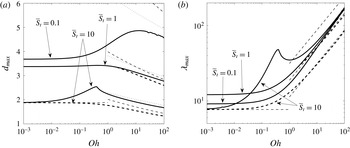
These two quantities are plotted in figure 4 for a few values of
 $\overline{S}_{t}$
as a function of
 $\mathit{Oh}$
. What is particularly remarkable is that the drop diameter remains mostly constant in the full interval
 $10^{-3}<\mathit{Oh}<10^{2}$
whatever the noise level for both cases (figure 4
b). Yet, in this interval of
 $\mathit{Oh}$
, the breakup distance
 $z_{f}$
varies by a factor of 1000 (figure 3
a), while the wavelength varies by a factor of 20 or more (figure 4
a). In the case of background noise,
 $z_{f}$
and
 $\unicode[STIX]{x1D706}_{max}$
increase with
 $\mathit{Oh}$
. We observe the same evolution in the case of noise excitation for small
 $\overline{S}_{t}$
. However, the curves of both cases depart from each other for large values of
 $\overline{S}_{t}$
(for instance
 $\overline{S}_{t}=10$
) with a surprising local peak for case (i) close to
 $\mathit{Oh}\approx 0.3$
. As we shall see in § 4, this peak is associated with a larger damping of the perturbation outside the instability range for moderate
 $\mathit{Oh}$
.
Wavelength at breakup (a) and resulting droplet diameter (b) versus
 $\mathit{Oh}$
for background noise (dashed lines) and nozzle excitation (solid lines). The different curves correspond to the transition level
 $\bar{S}_{t}=0.1$
, 1, 10. The thin dashed lines correspond to the asymptotic expressions for small and large
 $\mathit{Oh}$
.

In figures 3 and 4, we have also plotted the asymptotic behaviours of the different quantities obtained for large
 $\mathit{Oh}$
and small
 $\mathit{Oh}$
. The details of the derivation are provided in appendix A. We provide below the final result only.
3.1 Large viscosity (large
$\mathit{Oh}$
)

In the viscous régime (
 $\mathit{Oh}\gg 1$
), the position
 $z_{f}$
of breakup strongly increases with
 $\mathit{Oh}$
, and converges to the asymptotic curve (deduced from (A 10) and (A 12))
 $$\begin{eqnarray}z_{f}/z_{o}\sim \left(\frac{9}{2\sqrt{2}}\right)^{4/3}\overline{S}_{t}^{4/3}\mathit{Oh}^{4/3}\end{eqnarray}$$
for both cases (i) and (ii) if
 $1\ll z_{f}/z_{o}\ll \mathit{Oh}^{4}$
. The variation in terms of
 $\mathit{Bo}$
and
 $Q$
can be obtained using (3.1) and (2.12).
This scaling law, which was also derived by Javadi et al. (Reference Javadi, Eggers, Bonn, Habibi and Ribe2013), expresses that breakup occurs when the local capillary instability growth rate overcomes the stretching rate of the jet. Indeed, and coming back to dimensional quantities, the velocity and local radius vary far from the nozzle as
 $U_{0}\sim \sqrt{2gz}$
and
 $h\sim \sqrt{Q^{\ast }}/(2gz)^{1/4}$
respectively, where
 $Q^{\ast }=U_{0}h^{2}$
is the dimensional flow rate. The local stretching rate is then given by
 $\unicode[STIX]{x2202}_{z}U_{0}\sim \sqrt{g/(2z)}$
while the viscous capillary growth rate based on the current radius is of order
 $\unicode[STIX]{x1D6FE}/(\unicode[STIX]{x1D702}h)=\unicode[STIX]{x1D6FE}(2gz)^{1/4}/(\unicode[STIX]{x1D702}\sqrt{Q^{\ast }})$
. The latter overcomes the former at a distance
 $z_{f}$
of order
 $(\unicode[STIX]{x1D702}/\unicode[STIX]{x1D6FE})^{4/3}g^{1/3}(Q^{\ast })^{2/3}$
. In terms of dimensionless parameters, this gives
 $$\begin{eqnarray}z_{f}/h_{0}\propto \mathit{Oh}^{4/3}\mathit{Bo}^{1/3}Q^{2/3},\end{eqnarray}$$
which is essentially the scaling deduced from (3.5) if one remembers that
 $\overline{S}_{t}\propto \mathit{Bo}/Q$
and
 $z_{o}\propto Q^{2}/\mathit{Bo}$
.
In this viscous régime, the most dangerous frequencies are not the same in cases (i) and (ii). This implies that the wavelength
 $\unicode[STIX]{x1D706}_{max}$
at the point of transition and the droplet diameter
 $d_{max}$
are also different. For case (i), we obtain from (A 9) and (3.5)
 $$\begin{eqnarray}\overline{\unicode[STIX]{x1D714}}_{max}^{(a)}\sim \unicode[STIX]{x1D6FC}_{a}\overline{S}_{t}^{2/3}\mathit{Oh}^{1/6},\quad \text{with}~\unicode[STIX]{x1D6FC}_{a}=\frac{3^{3/4}}{2^{7/4}}\approx 0.678,\end{eqnarray}$$
which gives
 $$\begin{eqnarray}\displaystyle & \displaystyle \unicode[STIX]{x1D706}_{max}^{(a)}\sim \unicode[STIX]{x1D6FD}_{a}\mathit{Oh}^{1/2},\quad \text{with}~\unicode[STIX]{x1D6FD}_{a}=4\unicode[STIX]{x03C0}3^{1/4}\approx 16.54, & \displaystyle\end{eqnarray}$$
 $$\begin{eqnarray}\displaystyle & \displaystyle d_{max}^{(a)}\sim \unicode[STIX]{x1D6FE}_{a}\overline{S}_{t}^{-2/9}\mathit{Oh}^{-1/18},\quad \text{with}~\unicode[STIX]{x1D6FE}_{a}=\unicode[STIX]{x03C0}^{1/3}3^{1/12}2^{15/12}\approx 3.82. & \displaystyle\end{eqnarray}$$
 $$\begin{eqnarray}\overline{\unicode[STIX]{x1D714}}_{max}^{(b)}\sim \unicode[STIX]{x1D6FC}_{b}\overline{S}_{t}^{8/9}\mathit{Oh}^{2/9},\quad \text{with}~\unicode[STIX]{x1D6FC}_{b}=\frac{3}{2^{7/3}}\approx 0.595,\end{eqnarray}$$
which gives
 $$\begin{eqnarray}\displaystyle & \displaystyle \unicode[STIX]{x1D706}_{max}^{(b)}\sim \unicode[STIX]{x1D6FD}_{b}\overline{S}_{t}^{-2/9}\mathit{Oh}^{4/9},\quad \text{with}~\unicode[STIX]{x1D6FD}_{b}=2^{31/12}\unicode[STIX]{x03C0}\approx 18.83, & \displaystyle\end{eqnarray}$$
 $$\begin{eqnarray}\displaystyle & \displaystyle d_{max}^{(b)}\sim \unicode[STIX]{x1D6FE}_{b}\overline{S}_{t}^{-8/27}\mathit{Oh}^{-2/27},\quad \text{with}~\unicode[STIX]{x1D6FE}_{b}=\unicode[STIX]{x03C0}^{1/3}2^{13/9}\approx 3.99. & \displaystyle\end{eqnarray}$$
 $\unicode[STIX]{x1D706}_{max}$
the most unstable local wavelength at
 $z_{f}$
. As will be shown in § 5, this fails in making the correct predictions, precisely because it ignores the stretching history of the fluid particles and of the corresponding unstable modes. Equation (3.6) is thus consistent with a local argument, but the local argument does not incorporate the whole truth.
3.2 Low viscosity (small
$\mathit{Oh}$
)

In the weakly viscous régime (
 $\mathit{Oh}\ll 1$
), both noise and nozzle excitations are expected to give the same breakup distance
 $z_{f}$
. This distance is well approximated by
 $$\begin{eqnarray}z_{f}/z_{o}\approx \unicode[STIX]{x1D702}_{0}\overline{S}_{t}^{8/7},\quad \text{with}~\unicode[STIX]{x1D702}_{0}\approx 3.45,\end{eqnarray}$$
when
 $z_{f}/z_{o}>3.74$
, that is
 $\overline{S}_{t}>1.32$
.
Again, as in the previous viscous limit, this scaling law expresses that breakup occurs when the local capillary instability growth rate overcomes the stretching rate. The local jet stretching rate is still
 $\unicode[STIX]{x2202}_{z}U_{0}\sim \sqrt{g/(2z)}$
while the inviscid capillary growth rate based on the current radius is now of order
 $\sqrt{\unicode[STIX]{x1D6FE}/\unicode[STIX]{x1D70C}h^{3}}=\sqrt{\unicode[STIX]{x1D6FE}/\unicode[STIX]{x1D70C}}(2gz)^{3/8}/(Q^{\ast })^{3/4}$
. The latter overcomes the former at a distance of order
 $(Q^{\ast })^{6/7}g^{1/7}(\unicode[STIX]{x1D70C}/\unicode[STIX]{x1D6FE})^{4/7}$
. In terms of dimensionless parameters, this gives
 $$\begin{eqnarray}z_{f}/h_{0}\propto \mathit{Bo}^{1/7}Q^{6/7},\end{eqnarray}$$
which is essentially the scaling in (3.11) with
 $\overline{S}_{t}\propto \mathit{Bo}/Q$
and
 $z_{o}\propto Q^{2}/\mathit{Bo}$
.
In this régime, the most dangerous frequency is also the same in both cases and is given by
 $$\begin{eqnarray}\overline{\unicode[STIX]{x1D714}}_{max}=\unicode[STIX]{x1D6FC}_{0}\overline{S}_{t}^{6/7},\quad \text{with}~\unicode[STIX]{x1D6FC}_{0}\approx 0.79,\end{eqnarray}$$
which gives
 $$\begin{eqnarray}\displaystyle & \displaystyle \unicode[STIX]{x1D706}_{max}\sim \unicode[STIX]{x1D6FD}_{0}\overline{S}_{t}^{-2/7},\quad \text{with}~\unicode[STIX]{x1D6FD}_{0}\approx 14.82, & \displaystyle\end{eqnarray}$$
 $$\begin{eqnarray}\displaystyle & \displaystyle d_{max}\sim \unicode[STIX]{x1D6FE}_{0}\overline{S}_{t}^{-2/7},\quad \text{with}~\unicode[STIX]{x1D6FE}_{0}\approx 3.63. & \displaystyle\end{eqnarray}$$
4 Comparison with three-dimensional predictions
In this section, we focus on the régime of intermediate values of
 $\mathit{Oh}$
for which the asymptotic expressions do not apply. We address the peculiar behaviour of the optimal perturbation in the case of nozzle excitation in this régime. In figure 4(a,b), we have seen that for
 $\overline{S}_{t}=10$
both
 $\unicode[STIX]{x1D706}_{max}$
and
 $d_{max}$
exhibit a surprising kink around
 $\mathit{Oh}\approx 0.3$
. The same non-monotonic behaviour has also been observed in the breakup distance
 $z_{f}/z_{0}$
as a function of
 $\mathit{Oh}$
(see figure 3
a). These surprising behaviours are associated with the particular properties of the perturbations outside the instability domain. Indeed, for large
 $\overline{S}_{t}$
, the optimal perturbation is obtained for
 $\overline{\unicode[STIX]{x1D714}}_{max}>1$
. The local wavenumber of the perturbation, which is
 $\overline{\unicode[STIX]{x1D714}}$
at the nozzle, is then larger than 1 close to the nozzle, that is in the stable régime (see figure 5
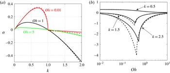
a). The optimal perturbation excited from the nozzle is thus first spatially damped before becoming spatially amplified. This damping régime explains the smaller gain obtained by nozzle excitation compared with background noise. It turns out that the strength of this damping is not monotonic with respect to
 $\mathit{Oh}$
and exhibits a peak for an intermediate value of
 $\mathit{Oh}$
. Such a peak is illustrated in figure 5, where we have plotted the (local) temporal growth rate of the perturbation versus
 $\mathit{Oh}$
for a few values of the (local) wavenumber. We do observe that for the values of
 $k$
satisfying
 $k\geqslant 1$
, that is outside the instability band, the local growth rate exhibits a negative minimum for
 $\mathit{Oh}$
between 0.1 and 1.
Comparison of 1D and 3D local dispersion relations. Solid line: 1D dispersion relation. Dashed line: 3D dispersion relation for axisymmetric modes. (a) Temporal growth rate versus the wavenumber
 $k$
for various
 $\mathit{Oh}$
. (b) Temporal growth rate versus
 $\mathit{Oh}$
for fixed wavelengths.

The presence of this damping régime naturally questions the validity of our one-dimensional (1D) model. The 1D model is indeed known to correctly describe the instability characteristics of three-dimensional (3D) axisymmetric modes (Eggers & Villermaux Reference Eggers and Villermaux2008). However, no such results exist in stable régimes. In fact, the 1D dispersion relation departs from the 3D dispersion relation of axisymmetric modes when
 $k>1$
. This departure is visible in figure 5, where we have also plotted the local growth rate obtained from the 3D dispersion relation given in Chandrasekhar (Reference Chandrasekhar1961, p. 541). Significant differences are observed, but the 3D growth rates exhibit a similar qualitative behaviour as a function of
 $\mathit{Oh}$
. In particular, there is still a damping rate extremum in the interval
 $0.1<\mathit{Oh}<1$
. We can therefore expect a similar qualitative behaviour of the perturbation outside the instability range with the 3D model.
Characteristics of the response to nozzle excitation versus
 $\mathit{Oh}$
for various values of
 $\overline{S}_{t}$
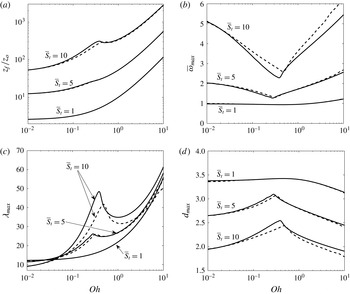
and two different stability models (solid line, 1D; dashed line, 3D axisymmetric). (a) Breakup distance. (b) Most dangerous frequency. (c) Wavelength at breakup. (d) Drop diameter.

In figure 6, we compare the optimization results for the nozzle excitation obtained with the 1D model with those obtained using the 3D dispersion relation of Chandrasekhar. This is done by replacing the function
 $\overline{S}$
in (2.27) by
 $$\begin{eqnarray}\overline{S}^{(3D)}(Z_{i},Z_{f},\overline{\unicode[STIX]{x1D714}},\mathit{Oh})=\sqrt{2}\mathit{Oh}\int _{Z_{i}}^{Z_{f}}(y^{2}(x,J)-x^{2})\,\text{d}z,\end{eqnarray}$$
where
 $$\begin{eqnarray}x=x(z,\overline{\unicode[STIX]{x1D714}})=\frac{\overline{\unicode[STIX]{x1D714}}}{z^{3/4}},\quad J=J(z,\mathit{Oh})=\frac{1}{\mathit{Oh}^{2}z^{1/4}},\end{eqnarray}$$
and
 $y=y(x,J)$
is given by
 $$\begin{eqnarray}2x^{2}(x^{2}+y^{2})\frac{I_{1}^{\prime }(x)}{I_{0}(x)}\left[1-\frac{2xy}{x^{2}+y^{2}}\frac{I_{1}(x)I_{1}^{\prime }(y)}{I_{1}(y)I_{1}^{\prime }(x)}\right]-(x^{4}-y^{4})=J\frac{xI_{1}(x)}{I_{0}(x)}(1-x^{2}).\end{eqnarray}$$
As expected, differences can be observed between the 1D and 3D results for the largest value of
 $\overline{S}_{t}$
(
 $\overline{S}_{t}=10$
). However, the trends remain the same. Close to
 $\mathit{Oh}\approx 0.3$
, the breakup distance exhibits a plateau, the frequency a minimum, the wavelength and the drop diameter a peak. These peaks have a smaller amplitude for the 3D dispersion relation and are slightly shifted to higher values of
 $\mathit{Oh}$
. For
 $\overline{S}_{t}=1$
, no difference between the two models is observed. This can be understood by the fact that the perturbation does not exhibit a period of damping for such a small value of
 $\overline{S}_{t}$
. The 1D model therefore perfectly describes the gain of 3D perturbations, which turns out to be the same as for background noise for
 $\mathit{Oh}<2$
(see figure 3
a).
5 Comparison with local predictions
In this section, our goal is to compare the results of the optimization procedure with predictions obtained from the local dispersion relation. We have seen in § 2 that the gain can be related to the local temporal growth rate of the perturbation along the jet (see expression (2.23)). Both the local capillary time scale
 $\unicode[STIX]{x1D70F}_{c_{l}}$
and the Ohnesorge number
 $\mathit{Oh}_{l}$
vary with
 $Z$
(see expressions (2.25b
), (2.25c
)). At a location
 $Z$
, the maximum temporal growth rate (normalized by the capillarity time at the nozzle) is given by
 $$\begin{eqnarray}\unicode[STIX]{x1D70E}_{l}^{max}(Z)=\frac{Z^{3/8}}{2\sqrt{2}+6\mathit{Oh}Z^{1/8}},\end{eqnarray}$$
and is reached for the wavelength (normalized by
 $h_{0}$
) (see Eggers & Villermaux Reference Eggers and Villermaux2008)
 $$\begin{eqnarray}\unicode[STIX]{x1D706}_{l}(Z)=\frac{2\unicode[STIX]{x03C0}}{Z^{1/4}}\sqrt{2+3\sqrt{2}\mathit{ Oh }Z^{1/8}}.\end{eqnarray}$$
If we form a drop from this perturbation wavelength at this location, we would then obtain a drop diameter (normalized by
 $h_{0}$
)
 $$\begin{eqnarray}d_{l}(Z)=\frac{(12\unicode[STIX]{x03C0})^{1/3}}{Z^{1/4}}\left(2+3\sqrt{2}\mathit{Oh}Z^{1/8}\right)^{1/6}.\end{eqnarray}$$
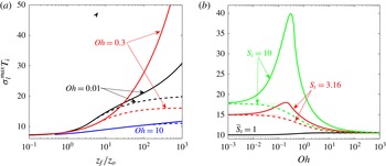
Maximum local temporal growth rate
 $\unicode[STIX]{x1D70E}_{l}^{max}$
normalized by the free fall time
 $T_{i}$
at the breakup location assuming breakup for a gain
 $\text{e}^{7}$
(solid line, nozzle excitation; dashed line, background noise). (a) Variation with respect to the breakup location
 $z_{f}/z_{o}$
for different
 $\mathit{Oh}$
. (b) Variation with respect to
 $\mathit{Oh}$
for different values of
 $\overline{S}_{t}$
. The dotted lines in (b) are the asymptotic predictions (5.5a
) and (5.5b
).

As the local growth rate increases downstream, a simple upper bound of the gain is then obtained by taking the exponential of the product of the maximum growth rate by the time
 $T_{i}$
needed to reach the chosen location. The time
 $T_{i}$
is the free fall time given by
 $$\begin{eqnarray}T_{i}=\frac{Q}{\mathit{Bo}}(\sqrt{Z}-1).\end{eqnarray}$$
In figure 7, we have plotted the product
 $\unicode[STIX]{x1D70E}_{l}^{max}T_{i}$
at the location predicted for the transition assuming that a gain
 $\text{e}^{7}$
is needed for such a transition. In figure 7(a), this quantity is plotted as a function of the transition location
 $z_{f}/z_{o}$
. As expected, we obtain the chosen value for the transition (i.e. 7) for small
 $z_{f}/z_{o}$
. For large
 $z_{f}/z_{o}$
, the product
 $\unicode[STIX]{x1D70E}_{l}^{max}T_{i}$
also goes to a constant for background noise whatever the Ohnesorge number. However, it has a contrasted behaviour for nozzle excitation, with an important increase with
 $z_{f}/z_{o}$
for the value
 $\mathit{Oh}=0.3$
.
In figure 7(b),
 $\unicode[STIX]{x1D70E}_{l}^{max}T_{i}$
is plotted as a function of
 $\mathit{Oh}$
, for different values of
 $\overline{S}_{t}$
, that is for different values of the ratio
 $\mathit{Bo}/Q$
in view of (3.1). For large and small
 $\mathit{Oh}$
, we recover the estimates deduced using (3.5) and (3.11),
 $$\begin{eqnarray}\displaystyle & \displaystyle \unicode[STIX]{x1D70E}_{l}^{max}T_{i}\sim 10.5\quad \text{as}~\mathit{Oh}\rightarrow \infty , & \displaystyle\end{eqnarray}$$
 $$\begin{eqnarray}\displaystyle & \displaystyle \unicode[STIX]{x1D70E}_{l}^{max}T_{i}\sim 20.68-11.14\overline{S}_{t}^{-4/7}\quad \text{as}~\mathit{Oh}\rightarrow 0. & \displaystyle\end{eqnarray}$$
 $\unicode[STIX]{x1D70E}_{l}^{max}T_{i}$
varies smoothly between these two extreme values. A completely different evolution is observed for nozzle excitation: a local peak forms between
 $0.1<\mathit{Oh}<1$
with an amplitude increasing with
 $\overline{S}_{t}$
. This phenomenon is related to the damping of the optimal perturbation discussed in the previous section. We have indeed seen that for nozzle excitation, large gain (that is large
 $\overline{S}_{t}$
) is obtained for perturbations exhibiting a damping period prior to their growth. Thus, the growth has to compensate a loss of amplitude. As the damping is strongest for intermediate
 $\mathit{Oh}$
, the transition is pushed the farthest for these values, explaining the largest growth of the
 $\mathit{Oh}=0.3$
curve in figure 7(a) and the peaks of figure 7(b).
We have seen that the optimal procedure provides a wavelength and a droplet size as a function of
 $Z$
and
 $\mathit{Oh}$
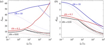
only. These quantities are compared with the local estimates (5.2) and (5.3) in figure 8. Both nozzle excitation (solid lines) and background noise (dashed lines) are considered for
 $\mathit{Oh}=0.01$
, 0.3 and 10. We observe that the local predictions (dotted lines) always underestimate the wavelength and the drop diameter. For the wavelength, the ratio with the local estimate typically increases with
 $z_{f}/z_{o}$
and
 $\mathit{Oh}$
. The gap is the strongest for the nozzle excitation case, especially for intermediate
 $\mathit{Oh}$
(see the curve for
 $\mathit{Oh}=0.3$
), for which the local estimate is found to underestimate the wavelength by a factor as high as 25 for
 $z_{f}/z_{o}=10^{3}$
.
Wavelength at breakup (a) and drop diameter (b) versus the breakup location
 $z_{f}/z_{o}$
for various values of
 $\mathit{Oh}$
(solid line, nozzle excitation; dashed line, background noise).

In contrast to the wavelength, the drop diameter follows the same trend as the local prediction as a function of
 $z_{f}/z_{o}$
. For both noise excitation and background noise, the diameter decreases with the breakup location.
For large or small
 $\mathit{Oh}$
, the behaviours of the wavelength and drop diameter obtained by the optimization procedure and local consideration can be directly compared using the results obtained in appendix A. For large
 $\mathit{Oh}$
, the local prediction reads
 $$\begin{eqnarray}\displaystyle & \displaystyle \unicode[STIX]{x1D706}_{l}/h_{0}\sim \unicode[STIX]{x1D6FD}_{l}\mathit{Oh}^{1/2}Z_{f}^{-3/16},\quad \text{with}~\unicode[STIX]{x1D6FD}_{l}=2\unicode[STIX]{x03C0}2^{1/4}\sqrt{3}\approx 12.94, & \displaystyle\end{eqnarray}$$
 $$\begin{eqnarray}\displaystyle & \displaystyle d_{l}/h_{0}\sim \unicode[STIX]{x1D6FE}_{l}\mathit{Oh}^{1/6}Z_{f}^{-11/49},\quad \text{with}~\unicode[STIX]{x1D6FE}_{l}=(2\unicode[STIX]{x03C0})^{1/3}(3\sqrt{2})^{1/6}\approx 2.35, & \displaystyle\end{eqnarray}$$
 $$\begin{eqnarray}\displaystyle & \displaystyle \unicode[STIX]{x1D706}_{max}^{(a)}/h_{0}\sim \unicode[STIX]{x1D6FD}^{(a)}\mathit{Oh}^{1/2},\quad \text{with}~\unicode[STIX]{x1D6FD}^{(a)}\approx 16.54, & \displaystyle\end{eqnarray}$$
 $$\begin{eqnarray}\displaystyle & \displaystyle \unicode[STIX]{x1D706}_{max}^{(b)}/h_{0}\sim \unicode[STIX]{x1D6FD}^{(b)}\mathit{Oh}^{2/3}Z_{f}^{-1/6},\quad \text{with}~\unicode[STIX]{x1D6FD}^{(b)}\approx 22.83, & \displaystyle\end{eqnarray}$$
 $$\begin{eqnarray}\displaystyle & \displaystyle d_{max}^{(a)}/h_{0}\sim \unicode[STIX]{x1D6FE}^{(a)}\mathit{Oh}^{1/6}Z_{f}^{-1/6},\quad \text{with}~\unicode[STIX]{x1D6FE}^{(a)}\approx 4.63, & \displaystyle\end{eqnarray}$$
 $$\begin{eqnarray}\displaystyle & \displaystyle d_{max}^{(b)}/h_{0}\sim \unicode[STIX]{x1D6FE}^{(b)}\mathit{Oh}^{2/9}Z_{f}^{-2/9},\quad \text{with}~\unicode[STIX]{x1D6FE}^{(b)}\approx 5.16. & \displaystyle\end{eqnarray}$$
 $\mathit{Oh}$
, the local estimates are
 $$\begin{eqnarray}\displaystyle & \displaystyle \unicode[STIX]{x1D706}_{l}^{nv}/h_{0}\sim \unicode[STIX]{x1D6FD}_{l}^{nv}Z_{f}^{-1/4},\quad \text{with}~\unicode[STIX]{x1D6FD}_{l}^{nv}\approx 2\unicode[STIX]{x03C0}\sqrt{2}\approx 8.88, & \displaystyle\end{eqnarray}$$
 $$\begin{eqnarray}\displaystyle & \displaystyle d_{l}^{nv}/h_{0}\sim \unicode[STIX]{x1D6FE}_{l}^{nv}Z_{f}^{-1/4},\quad \text{with}~\unicode[STIX]{x1D6FE}_{l}^{nv}=(12\unicode[STIX]{x03C0})^{1/3}(2)^{1/6}\approx 3.76, & \displaystyle\end{eqnarray}$$
 $Z_{f}>4.74$
(see appendix A)
 $$\begin{eqnarray}\displaystyle & \displaystyle \unicode[STIX]{x1D706}_{max}/h_{0}\sim \unicode[STIX]{x1D6FD}^{nv}Z_{f}^{-1/4},\quad \text{with}~\unicode[STIX]{x1D6FD}^{nv}\approx 20.20, & \displaystyle\end{eqnarray}$$
 $$\begin{eqnarray}\displaystyle & \displaystyle d_{max}/h_{0}\sim \unicode[STIX]{x1D6FE}^{nv}Z_{f}^{-1/4},\quad \text{with}~\unicode[STIX]{x1D6FE}^{nv}\approx 4.94. & \displaystyle\end{eqnarray}$$
6 Applications
We now apply the results to a realistic configuration obtained from a nozzle of radius
 $h_{0}=1$
mm in a gravity field with
 $g=9.81~\text{m}~\text{s}^{-2}$
. We consider three fluids: water (at
 $20^{\circ }$
), for which
 $\unicode[STIX]{x1D6FE}\approx 72\times 10^{-3}~\text{N}~\text{m}^{-1}$
,
 $\unicode[STIX]{x1D708}\approx 10^{-6}~\text{m}^{2}~\text{s}^{-1}$
, and two silicone oils of surface tension
 $\unicode[STIX]{x1D6FE}\approx 21\times 10^{-3}~\text{N}~\text{m}^{-1}$
and of viscosity
 $\unicode[STIX]{x1D708}\approx 5\times 10^{-5}~\text{m}^{2}~\text{s}^{-1}$
and
 $\unicode[STIX]{x1D708}\approx 3\times 10^{-4}~\text{m}^{2}~\text{s}^{-1}$
. For these three fluids, we take
 $\unicode[STIX]{x1D70C}\approx 10^{3}~\text{kg}~\text{m}^{-3}$
as a fair order of magnitude.
For water, we obtain
 $\mathit{Oh}=3.7\times 10^{-3}$
,
 $\mathit{Bo}=0.13$
and a parameter
 $Q=3.72u_{0}$
, with the velocity
 $u_{0}$
at the nozzle expressed in
 $\text{m}~\text{s}^{-1}$
. For the silicone oils, we get
 $\mathit{Bo}=0.46$
and
 $Q=6.9u_{0}$
and two values of
 $\mathit{Oh}$
:
 $\mathit{Oh}=0.46$
and
 $\mathit{Oh}=2$
. The conditions of validity (2.9a
)–(2.9c
) of the inertial solution then require
 $u_{0}$
to be (much) larger than
 $u_{c}=0.26~\text{m}~\text{s}^{-1}$
for the water and
 $u_{c}=0.15~\text{m}~\text{s}^{-1}$
for the silicone oils.
Characteristics at breakup by nozzle excitation or background noise for a jet of radius
 $h_{0}=1$
mm assuming that breakup occurs when the perturbation gain has reached
 $\text{e}^{S_{t}}$
(solid lines, nozzle excitation with
 $S_{t}=4$
; dot–dash lines, nozzle excitation with
 $S_{t}=4$
using the 3D dispersion relation; dashed lines, background noise with
 $S_{t}=7$
; black lines, water; red lines, silicone oil of
 $\unicode[STIX]{x1D708}=5\times 10^{-5}~\text{m}^{2}~\text{s}^{-1}$
(SO50); green lines, silicone oil of
 $\unicode[STIX]{x1D708}=3\times 10^{-4}~\text{m}^{2}~\text{s}^{-1}$
(SO300)). (a) Breakup location; (b) most dangerous frequency; (c) wavelength at breakup; (d) drop diameter.

In figure 9, we have plotted the theoretical predictions for the breakup location, the frequency, the wavelength and the drop diameter as the fluid velocity at the nozzle is varied from
 $u_{c}$
to 10
 $u_{c}$
, that is for
 $Q$
varying from 1 to 10. We have chosen
 $S_{t}=7$
for the background noise transition and
 $S_{t}=4$
for the transition by the nozzle excitation. A smaller value of
 $S_{t}$
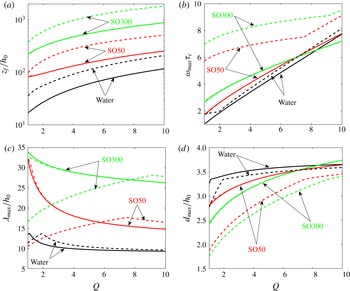
has been chosen for the nozzle excitation to describe controlled conditions of forcing. Figure 9(a) shows that for the three fluids the transition by the nozzle excitation can be reached before the background noise transition. The values obtained for the breaking length are comparable to the experimental values reported in Javadi et al. (Reference Javadi, Eggers, Bonn, Habibi and Ribe2013). They measured a normalized breaking length of order 100–150 for silicone oil of
 $\unicode[STIX]{x1D708}\approx 5\times 10^{-5}~\text{m}^{2}~\text{s}^{-1}$
from a nozzle of the same diameter for flow rates ranging from
 $Q=0.5$
to
 $Q=1.3$
.
Figure 9(b) provides the most dangerous frequency of the excitation. For the three cases, the frequency for the nozzle excitation is relatively close to the neutral frequency
 $Q$
of the jet at the nozzle. For both silicone oils, this frequency is, however, much smaller than the frequency obtained by the background noise transition, especially for small
 $Q$
.
The breakup wavelength shown in figure 9(c) exhibits a different behaviour with respect to the flow rate
 $Q$
for the nozzle excitation and the background noise. It decreases monotonically with
 $Q$
for the noise excitation while it increases for the background noise up to an extremum before starting to decrease. For the three fluids, noise excitation provides a larger wavelength than background noise for small
 $Q$
, but the opposite is observed above a critical value of
 $Q$
which increases with
 $\mathit{Oh}$
. It should be noted that for small
 $Q$
, the wavelengths obtained for noise excitation are comparable for both silicone oils. Both curves would even cross if a larger value of
 $S_{t}$
was considered. This property is related to the non-monotonic behaviour of the breakup wavelength already discussed above (see figure 6
c).
In contrast to the wavelength, the droplet size (figure 9
d) does not change much with
 $Q$
and is comparable for the three fluids. Nozzle excitation provides larger droplets, but this effect is significant for the smallest values of
 $Q$
only.
Finally, it should be noted that the differences between the 1D and 3D predictions for the nozzle excitation are barely visible. A very small departure of the wavelength curves can be seen for the silicone oils only. This confirms both the usefulness and the validity of the 1D model.
7 Conclusion and final remarks
At the end of this detailed study, we are now in a position to answer the questions raised in the introduction. The breakup distance from the orifice of a jet falling by its own weight can indeed be understood by comparing two time scales. The relevant time scales are the capillary destabilization time (viscous, or not) based on the local jet radius, and the inverse of the local jet stretching rate. Breakup occurs, in both viscous and inviscid régimes, as discussed in § 3, when the latter overcomes the former, a fact that was already known (Villermaux Reference Villermaux2012; Javadi et al.
Reference Javadi, Eggers, Bonn, Habibi and Ribe2013). However, we have also learned that this aspect is only a tiny piece of the problem as a whole. This simple local rule, if naively extended to estimation of the wavelength of the perturbation breaking the jet, would predict that the wavelength is proportional to the local jet radius in the inviscid case, for instance. This prediction was found to always underestimate the wavelength at breakup. The most dangerous wavelength and the drop diameter account for the stretching history of the fluid particles as they travel along the jet; this is the reason why their values are different depending on whether the perturbations are introduced at the jet nozzle only or through a background noise affecting the jet all along its extension. An optimal theory computing the gain of every mode as the jet deforms and accelerates was thus necessary to answer the – seemingly simple – question of its breakup. It has, in addition, revealed the existence of an unexpected non-monotonic dependence of the most dangerous wavelength
 $\unicode[STIX]{x1D706}_{max}$
with respect to
 $\mathit{Oh}$
.
We have also provided quantitative results assuming that a spatial gain of
 $\text{e}^{7}$
of the linear perturbations is sufficient for breakup. This value of the critical gain is an ad hoc criterion which assumes a particular level of noise and which neglects the possible influence of the nonlinear effects. It would be interesting to test this criterion with experimental data.
Our analysis has focused on a capillary jet whose base state is in an inertial régime. Close to the nozzle, especially if the flow rate is small, a viscous dominated régime is expected (Senchenko & Bohr Reference Senchenko and Bohr2005). We have not considered such a régime here. However, a similar WKBJ analysis could a priori be performed with a base flow obtained by resolving the more general equations (2.2) if the jet variation scale remains large compared with the perturbation wavelength. However, far from the nozzle, the jet always becomes inertial. The growth of the perturbation is therefore expected to be the same as described above. For this reason, the optimal perturbation obtained from background noise could be the same. Indeed, we have seen that in order to reach a large gain (
 $\overline{S}_{t}>5$
or so), the optimal perturbation should be introduced far from the nozzle. If the jet is in the inertial régime at this location, the same gain is then obtained. This point was already noticed in Javadi et al. (Reference Javadi, Eggers, Bonn, Habibi and Ribe2013).
For nozzle excitation, the entire evolution of the jet contributes to the optimal perturbation. We have seen that large gains (
 $\overline{S}_{t}>5$
) are obtained by perturbations that exhibit a spatial damping before starting to grow. We have also seen that this damping régime is only qualitatively described by the 1D model. We do not expect a better description if the jet is dominated by viscous effects. Moreover, it is known that in this régime non-parallel effects are also important close to the nozzle (Rubio-Rubio et al.
Reference Rubio-Rubio, Sevilla and Gordillo2013), which invalidates the WKBJ approach. For this régime, it would be interesting to perform an optimal stability analysis using more advanced tools (Schmid Reference Schmid2007) to take into account non-parallel effects and non-modal growth.
It should be noted finally that we have computed the perturbation gain by considering the exponential terms of the WKBJ approximation only. A better estimate could readily be obtained by considering the complete expression of the WKBJ approximation. This expression, which has been provided in appendix B, involves an amplitude factor that contains all of the other contributions affecting the growth of the perturbation. Different expressions are obtained for
 $A$
and
 $u$
, which, in particular, implies that different gains are obtained for the velocity and the jet radius. It is important to mention that the other contributions are not limited to a simple correcting factor associated with the local stretching (Tomotika Reference Tomotika1936; Eggers & Villermaux Reference Eggers and Villermaux2008). Other contributions associated with the
 $z$
-dependence of the local wavenumber and local jet profile are equally important, leading to expressions that are not simple even in the large- or small-
 $\mathit{Oh}$
limit.
Acknowledgement
We acknowledge support from the French Agence Nationale de la Recherche under the ANR FISICS project ANR-15-CE30-0015-03.
Appendix A. Asymptotic régimes
In this appendix, we provide asymptotic expressions for
 $\overline{S}_{max}$
and
 $\overline{\unicode[STIX]{x1D714}}_{max}$
in the viscous and inviscid régimes, that is for
 $\mathit{Oh}\rightarrow \infty$
and
 $\mathit{Oh}\rightarrow 0$
respectively.
A.1 Maximum gain in the viscous régime
$(\mathit{Oh}\rightarrow \infty )$

When
 $\mathit{Oh}\rightarrow \infty$
, the expression of the integrand in (2.27) can be simplified, and in the whole domain of integration, we can use the approximation
 $$\begin{eqnarray}\sqrt{1-\overline{\unicode[STIX]{x1D714}}^{2}z^{-3/2}+\frac{9\mathit{Oh}^{2}\overline{\unicode[STIX]{x1D714}}^{2}}{2}z^{-5/4}}\sim \sqrt{1+\frac{9\mathit{Oh }^{2}\overline{\unicode[STIX]{x1D714}}^{2}}{2}z^{-5/4}}-\frac{\overline{\unicode[STIX]{x1D714}}^{2}z^{-3/2}}{2\sqrt{1+{\displaystyle \frac{9\mathit{Oh }^{2}\overline{\unicode[STIX]{x1D714}}^{2}}{2}}z^{-5/4}}},\end{eqnarray}$$
such that (2.27) can be written as
 $$\begin{eqnarray}\overline{S}\sim \frac{\overline{S}_{1}(Z_{i},Z_{f},X_{\unicode[STIX]{x1D714}})}{\mathit{Oh}}-\frac{\overline{S}_{2}(Z_{i},Z_{f},X_{\unicode[STIX]{x1D714}})}{\mathit{Oh}^{3}},\end{eqnarray}$$
with
 $$\begin{eqnarray}\displaystyle & \displaystyle \overline{S}_{1}(Z_{i},Z_{f},X_{\unicode[STIX]{x1D714}})=X_{\unicode[STIX]{x1D714}}^{-3/4}\int _{Z_{i}X_{\unicode[STIX]{x1D714}}}^{Z_{f}X_{\unicode[STIX]{x1D714}}}X^{-7/8}\left(\sqrt{1+\frac{9}{2X^{5/4}}}-\frac{3}{\sqrt{2}X^{5/8}}\right)\text{d}X, & \displaystyle\end{eqnarray}$$
 $$\begin{eqnarray}\displaystyle & \displaystyle \overline{S}_{2}(Z_{i},Z_{f},X_{\unicode[STIX]{x1D714}})=X_{\unicode[STIX]{x1D714}}^{-1/2}\int _{Z_{i}X_{\unicode[STIX]{x1D714}}}^{Z_{f}X_{\unicode[STIX]{x1D714}}}\frac{X^{-19/8}}{2\sqrt{1+{\displaystyle \frac{9}{2X^{5/4}}}}}\,\text{d}X & \displaystyle\end{eqnarray}$$
 $$\begin{eqnarray}X_{\unicode[STIX]{x1D714}}=(\mathit{Oh}\overline{\unicode[STIX]{x1D714}})^{-8/5}.\end{eqnarray}$$
When
 $Z_{f}$
is not too large, we are in the following configuration.
(1)
 $Z_{i}X_{\unicode[STIX]{x1D714}}\ll 1$
and
 $Z_{f}X_{\unicode[STIX]{x1D714}}\ll 1$
. In this case, we can write
 $$\begin{eqnarray}\displaystyle & \displaystyle \overline{S}_{1}\sim \frac{2\sqrt{2}}{9}(Z_{f}^{3/4}-Z_{i}^{3/4})-\frac{X_{\unicode[STIX]{x1D714}}^{5/4}}{108\sqrt{2}}(Z_{f}^{2}-Z_{i}^{2})+O(X_{\unicode[STIX]{x1D714}}^{5/2}Z_{f}^{13/4}), & \displaystyle\end{eqnarray}$$
 $$\begin{eqnarray}\displaystyle & \displaystyle \overline{S}_{2}\sim \frac{2\sqrt{2}}{9X_{\unicode[STIX]{x1D714}}^{5/4}}\left(\frac{1}{Z_{i}^{3/4}}-\frac{1}{Z_{f}^{3/4}}\right)+O(Z_{f}^{1/2}), & \displaystyle\end{eqnarray}$$
 $$\begin{eqnarray}\overline{S}\sim \frac{2\sqrt{2}}{9\mathit{Oh}}(Z_{f}^{3/4}-1-\overline{\unicode[STIX]{x1D714}}^{2}+\overline{\unicode[STIX]{x1D714}}^{2}Z_{f}^{-3/4})-\frac{Z_{f}^{2}-1}{108\sqrt{2}\mathit{Oh}^{3}\overline{\unicode[STIX]{x1D714}}^{2}}+O\left(\frac{Z_{f}^{1/2}}{\mathit{Oh}^{3}},\frac{Z_{f}^{13/4}}{\mathit{Oh}^{5}\overline{\unicode[STIX]{x1D714}}^{4}}\right)\end{eqnarray}$$
in case (i) (nozzle excitation) and
 $$\begin{eqnarray}\overline{S}\sim \frac{2\sqrt{2}}{9\mathit{Oh}}(Z_{f}^{3/4}-2\overline{\unicode[STIX]{x1D714}}+\overline{\unicode[STIX]{x1D714}}^{2}Z_{f}^{-3/4})-\frac{Z_{f}^{2}-\overline{\unicode[STIX]{x1D714}}^{8/3}}{108\sqrt{2}\mathit{Oh}^{3}\overline{\unicode[STIX]{x1D714}}^{2}}+O\left(\frac{Z_{f}^{1/2}}{\mathit{Oh}^{3}},\frac{Z_{f}^{13/4}}{\mathit{Oh}^{5}\overline{\unicode[STIX]{x1D714}}^{4}}\right)\end{eqnarray}$$
in case (ii) (background noise) with
 $Z_{i}=\overline{\unicode[STIX]{x1D714}}^{4/3}$
.
In case (i), the maximum gain is obtained for
 $$\begin{eqnarray}\overline{\unicode[STIX]{x1D714}}_{max}^{(a)}\sim \left(\frac{Z_{f}^{2}-1}{48\mathit{Oh}^{2}(1-Z_{f}^{-3/4})}\right)^{1/4},\end{eqnarray}$$
that is
 $$\begin{eqnarray}\overline{\unicode[STIX]{x1D714}}_{max}^{(a)}\sim \frac{Z_{f}^{1/2}}{2~3^{1/4}\mathit{Oh}^{1/2}}\end{eqnarray}$$
for large
 $Z_{f}$
, and equals
 $$\begin{eqnarray}\overline{S}_{max}^{(a)}\sim \frac{2\sqrt{2}Z_{f}^{3/4}}{9\mathit{Oh}}\left(1-Z_{f}^{-3/4}-\frac{Z_{f}^{1/4}}{2\sqrt{3}\mathit{Oh}}\right)+O\left(\frac{Z_{f}^{1/4}}{\mathit{Oh}^{2}},\frac{Z_{f}^{5/4}}{\mathit{Oh}^{3}}\right).\end{eqnarray}$$
In case (ii), the maximum gain is obtained for
 $$\begin{eqnarray}\overline{\unicode[STIX]{x1D714}}_{max}^{(b)}\sim \frac{Z_{f}^{2/3}}{48^{1/3}\mathit{Oh}^{2/3}}\end{eqnarray}$$
and equals
 $$\begin{eqnarray}\overline{S}_{max}^{(b)}\sim \frac{2\sqrt{2}Z_{f}^{3/4}}{9\mathit{Oh}}\left(1-\frac{3^{2/3}}{2^{4/3}\mathit{Oh}^{2/3}Z_{f}^{1/12}}\right).\end{eqnarray}$$
The condition that
 $Z_{f}X_{\unicode[STIX]{x1D714}}^{max}\ll 1$
does not give any restriction in case (ii). However, it requires in case (i)
 $$\begin{eqnarray}Z_{f}\ll \mathit{Oh}^{4}.\end{eqnarray}$$
Maximum gain
 $\overline{S}_{max}^{(a)}$
(a) and most dangerous frequency
 $\overline{\unicode[STIX]{x1D714}}_{max}^{(a)}$
(b) of the perturbations excited at the nozzle as a function of the distance
 $Z_{f}$
from the nozzle (solid lines, numerical results; dashed and dotted lines, asymptotic results obtained for large
 $\mathit{Oh}$
for
 $Z_{f}\ll \mathit{Oh}^{4}$
(formulae (A 10) and (A 9)) and
 $Z_{f}\gg \mathit{Oh}^{4}$
(formulae (A 17) and (A 16)) respectively). Here,
 $\mathit{Oh}$
takes the values 1, 10, 100 and 1000.

When
 $Z_{f}\gg \mathit{Oh}^{4}$
, another limit has to be considered for case (i).
(2)
 $Z_{i}X_{\unicode[STIX]{x1D714}}\ll 1$
and
 $Z_{f}X_{\unicode[STIX]{x1D714}}\gg 1$
. In this limit, we have
 $$\begin{eqnarray}\displaystyle & \displaystyle \overline{S}_{1}\sim \frac{8Z_{f}^{8}}{X_{\unicode[STIX]{x1D714}}^{5/8}}-\frac{I_{o}}{X_{\unicode[STIX]{x1D714}}^{3/4}}, & \displaystyle\end{eqnarray}$$
 $$\begin{eqnarray}\displaystyle & \displaystyle \overline{S}_{2}\sim \frac{2\sqrt{2}}{9X_{\unicode[STIX]{x1D714}}^{5/4}Z_{i}^{3/4}}. & \displaystyle\end{eqnarray}$$
 $$\begin{eqnarray}\overline{S}\sim 8Z_{f}^{1/8}\overline{\unicode[STIX]{x1D714}}-I_{o}\overline{\unicode[STIX]{x1D714}}^{6/5}\mathit{Oh}^{1/5}-\frac{2\sqrt{2}\overline{\unicode[STIX]{x1D714}}^{2}}{9\mathit{Oh}}+O\left(\frac{Z_{f}^{1/2}}{\mathit{Oh}^{3}},\frac{Z_{f}^{13/4}}{\mathit{Oh}^{5}\overline{\unicode[STIX]{x1D714}}^{4}}\right),\end{eqnarray}$$
which is maximum for
 $$\begin{eqnarray}\overline{\unicode[STIX]{x1D714}}_{max}^{(a)}\sim 9\sqrt{2}\mathit{Oh}Z_{f}^{1/8}.\end{eqnarray}$$
The maximum gain equals
 $$\begin{eqnarray}\overline{S}_{max}^{(a)}\sim 36\sqrt{2}Z_{f}^{1/4}\mathit{Oh}.\end{eqnarray}$$
This estimate applies only when
 $Z_{f}\gg \mathit{Oh}^{4}$
.
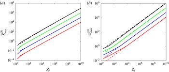
The asymptotic formulae are compared with numerical results in figure 10 for case (i) and figure 11 for case (ii). In both cases, we have plotted the maximum gain
 $\overline{S}_{max}$
and the most dangerous frequency (the frequency that provides the maximum gain) versus
 $Z_{f}$
for
 $\mathit{Oh}=1$
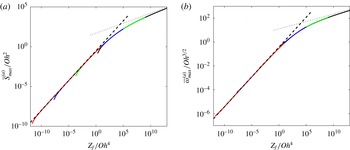
, 10, 100 and 1000. It is interesting to see that in case (i) the maximum gain and the most dangerous frequency both collapse onto a single curve when plotted as a function of the variable
 $Z_{f}/\mathit{Oh}^{4}$
with an adequate normalization (see figure 12).
Maximum gain
 $\overline{S}_{max}^{(b)}$
(a) and most dangerous frequency
 $\overline{\unicode[STIX]{x1D714}}_{max}^{(b)}$
(b) of the perturbations excited from background noise as a function of the distance
 $Z_{f}$
from the nozzle (solid lines, numerical results; dashed lines, asymptotic results (formulae (A 12) and (A 11))). From top to bottom,
 $\mathit{Oh}$
takes the values 1, 10, 100 and 1000.


A.2 Maximum gain in the inviscid régime
$(\mathit{Oh}\rightarrow 0)$

When
 $\mathit{Oh}$
is small, viscous effects come into play if we go sufficiently far away for the nozzle because the local Ohnesorge number increases algebraically with the distance to the nozzle.
Here, we shall assume that we remain inviscid in the whole domain of integration, that is
 $$\begin{eqnarray}\sqrt{1-\overline{\unicode[STIX]{x1D714}}^{2}z^{-3/2}+\frac{9\mathit{Oh}^{2}\overline{\unicode[STIX]{x1D714}}^{2}}{2}z^{-5/4}}-\frac{3}{\sqrt{2}}\overline{\unicode[STIX]{x1D714}}\mathit{Oh}z^{-5/8}\sim \sqrt{1-\overline{\unicode[STIX]{x1D714}}^{2}z^{-3/2}}.\end{eqnarray}$$
This is satisfied if
 $Z_{f}\ll \mathit{Oh}^{-8}$
. The gain can then be written as
 $$\begin{eqnarray}\overline{S}\sim Y_{\unicode[STIX]{x1D714}}^{-7/8}\int _{Z_{i}Y_{\unicode[STIX]{x1D714}}}^{Z_{f}Y_{\unicode[STIX]{x1D714}}}s^{-7/8}\sqrt{1-s^{-3/2}}\,\text{d}s,\end{eqnarray}$$
with
 $Y_{\unicode[STIX]{x1D714}}=\overline{\unicode[STIX]{x1D714}}^{-4/3}$
.
Because in the inviscid limit, perturbations are neutral when they do not grow, cases (i) and (ii) provide the same gain.
Maximum gain
 $\overline{S}_{max}$
(a) and most dangerous frequency
 $\overline{\unicode[STIX]{x1D714}}_{max}$
(b) of the perturbations excited from background noise (dashed lines) and at the nozzle (solid lines) as a function of the distance
 $z_{f}/z_{o}=Z_{f}-1$
from the nozzle. From bottom to top,
 $\mathit{Oh}$
takes the values 0.1, 0.01 and 0.001. The formulae (A 22) and (A 21) are indicated as solid grey lines in (a) and (b) respectively.

For
 $1<Z_{f}<Z_{f}^{c}\approx 4.74$
, the maximum gain is reached for
 $\overline{\unicode[STIX]{x1D714}}<1$
, i.e.
 $Y_{\unicode[STIX]{x1D714}}>1$
. The location
 $Z_{f}^{c}$
is given by the vanishing of
 $\unicode[STIX]{x2202}_{Y_{\unicode[STIX]{x1D714}}}\overline{S}$
for
 $Y_{\unicode[STIX]{x1D714}}=1$
and
 $Z_{i}=1$
:
 $$\begin{eqnarray}-\frac{7}{8}\int _{1}^{Z_{f}^{c}}s^{-7/8}\sqrt{1-s^{-3/2}}\,\text{d}s+(Z_{f}^{c})^{1/8}\sqrt{1-(Z_{f}^{c})^{-3/2}}=0.\end{eqnarray}$$
For
 $Z_{f}^{c}<Z_{f}\ll \mathit{Oh}^{-8}$
, the maximum gain is reached for
 $$\begin{eqnarray}\overline{\unicode[STIX]{x1D714}}_{max}\sim \left(\frac{Z_{f}}{Z_{f}^{c}}\right)^{3/4}\approx 0.311Z_{f}^{3/4}\end{eqnarray}$$
and equals
 $$\begin{eqnarray}\overline{S}_{max}=\unicode[STIX]{x1D6FD}Z_{f}^{7/8},\end{eqnarray}$$
where
 $$\begin{eqnarray}\unicode[STIX]{x1D6FD}=(Z_{f}^{c})^{-7/8}\int _{1}^{Z_{f}^{c}}s^{-7/8}\sqrt{1-s^{-3/2}}\,\text{d}s\approx 0.338.\end{eqnarray}$$
This estimate is compared with numerical values in figure 13. We do observe a convergence of the maximum gain and most dangerous frequency curves towards the inviscid limit as
 $\mathit{Oh}$
decreases. It should be noted, however, that the convergence is slower for nozzle excitation (case (i)).
Appendix B. WKBJ analysis
In this section, we provide the full expression of the WKBJ approximation of each downward propagative wave. Each wave is searched for in the form
 $$\begin{eqnarray}(u_{p},A_{p})=(v(Z),a(Z))\text{e}^{\text{i}z_{o}\int ^{Z}k(s)\,\text{d}s}\text{e}^{-\text{i}\unicode[STIX]{x1D714}t},\end{eqnarray}$$
where
 $k(Z)$
,
 $v(Z)$
and
 $a(Z)$
depend as the base flow on the slow spatial variable
 $Z=z/z_{o}+1$
,
 $z_{o}=Q^{2}/(2\mathit{Bo})$
being a large parameter.
If we plug expression (B 1) into (2.13), we get up to
 $O(1/z_{o}^{2})$
terms
 $$\begin{eqnarray}\displaystyle & \displaystyle (-\text{i}\unicode[STIX]{x1D714}+\text{i}kU_{0})a+\text{i}kA_{0}v=-\displaystyle \frac{1}{z_{o}}\displaystyle \frac{\unicode[STIX]{x2202}(aU_{0}+vA_{0})}{\unicode[STIX]{x2202}Z},\qquad & \displaystyle\end{eqnarray}$$
 $$\begin{eqnarray}\displaystyle & & \displaystyle \displaystyle (-\text{i}\unicode[STIX]{x1D714}+\text{i}kU_{0})v+3\mathit{Oh}k^{2}v-\displaystyle \frac{\text{i}k}{2A_{0}^{3/2}}(1-k^{2}A_{0})a\nonumber\\ \displaystyle & & \displaystyle \quad =-\displaystyle \frac{1}{z_{o}}\displaystyle \frac{\unicode[STIX]{x2202}(vU_{0})}{\unicode[STIX]{x2202}Z}+\displaystyle \frac{3\text{i}\mathit{Oh}}{z_{o}}\left(\displaystyle \frac{k}{A_{0}}\displaystyle \frac{\unicode[STIX]{x2202}A_{0}}{\unicode[STIX]{x2202}Z}v+2k\displaystyle \frac{\unicode[STIX]{x2202}v}{\unicode[STIX]{x2202}Z}+\displaystyle \frac{\unicode[STIX]{x2202}k}{\unicode[STIX]{x2202}Z}v+\frac{k}{A_{0}}\displaystyle \frac{\unicode[STIX]{x2202}U_{0}}{\unicode[STIX]{x2202}Z}a\right)\nonumber\\ \displaystyle & & \displaystyle \qquad -\,\displaystyle \frac{1}{4z_{o}A_{0}^{5/2}}\left(2A_{0}(1+3k^{2}A_{0})\displaystyle \frac{\unicode[STIX]{x2202}a}{\unicode[STIX]{x2202}Z}+\displaystyle \frac{\unicode[STIX]{x2202}A_{0}}{\unicode[STIX]{x2202}Z}(3-2k^{2}A_{0})a+6k\displaystyle \frac{\unicode[STIX]{x2202}k}{\unicode[STIX]{x2202}Z}A_{0}^{2}a\right).\qquad\end{eqnarray}$$
 $k(Z)$
. If we now replace
 $v$
on the right-hand side of (B 2a
) by its leading-order expression in terms of
 $a$
, we obtain an expression for
 $v$
valid up to
 $O(1/z_{o}^{2})$
terms:
 $$\begin{eqnarray}v=\frac{1}{kA_{0}}\left((\unicode[STIX]{x1D714}-kU_{0})a-\displaystyle \frac{1}{z_{o}}\displaystyle \frac{\unicode[STIX]{x2202}(\unicode[STIX]{x1D714}a/k)}{\unicode[STIX]{x2202}Z}\right).\end{eqnarray}$$
Plugging this expression into (B 2b
) with
 $U_{0}=Q/A_{0}$
, we obtain the following equation for
 $a(z)$
:
 $$\begin{eqnarray}R(Z)\displaystyle \frac{\unicode[STIX]{x2202}a}{\unicode[STIX]{x2202}Z}+\left(S(Z)\displaystyle \frac{\unicode[STIX]{x2202}A_{0}}{\unicode[STIX]{x2202}Z}+T(Z)\displaystyle \frac{\unicode[STIX]{x2202}k}{\unicode[STIX]{x2202}Z}\right)a=0,\end{eqnarray}$$
with
 $$\begin{eqnarray}\displaystyle & \displaystyle R(Z)=-2A_{0}k^{3}+6A_{0}^{2}k^{5}+4A_{0}^{3/2}k\left(\unicode[STIX]{x1D714}^{2}-3\mathit{Oh}\text{i}k^{2}\unicode[STIX]{x1D714}+\displaystyle \frac{Qk^{2}(-Q+6\text{i}\mathit{Oh}A_{0}k^{3})}{A_{0}^{2}}\right),\qquad & \displaystyle\end{eqnarray}$$
 $$\begin{eqnarray}\displaystyle & \displaystyle S(Z)=\displaystyle \frac{-8Q\unicode[STIX]{x1D714}k^{2}A_{0}+3k^{2}(4Q^{2}+A_{0}^{3/2}+4\text{i}\mathit{Oh}\unicode[STIX]{x1D714}A_{0}^{2})-24\text{i}\mathit{Oh}QA_{0}k^{4}-2A_{0}^{5/2}k^{5}}{A_{0}^{3/2}},\qquad & \displaystyle\end{eqnarray}$$
 $$\begin{eqnarray}\displaystyle & \displaystyle T(Z)=2A_{0}^{1/2}(-2\unicode[STIX]{x1D714}^{2}A_{0}+6\text{i}\mathit{Oh}Qk^{3}+3A_{0}^{3/2}k^{4}).\qquad & \displaystyle\end{eqnarray}$$
For large
 $Q$
, it can be simplified for the downward propagating wavenumbers using
 $\unicode[STIX]{x1D714}=\overline{\unicode[STIX]{x1D714}}Q$
and
 $k\sim \overline{\unicode[STIX]{x1D714}}A_{0}+k_{1}/Q$
as
 $$\begin{eqnarray}(-2k_{1}A_{0}+3\text{i}\overline{\unicode[STIX]{x1D714}}^{2}\mathit{Oh}A_{0}^{4})\displaystyle \frac{\unicode[STIX]{x2202}a}{\unicode[STIX]{x2202}Z}+\left(5k_{1}\displaystyle \frac{\unicode[STIX]{x2202}A_{0}}{\unicode[STIX]{x2202}Z}-A_{0}\displaystyle \frac{\unicode[STIX]{x2202}k_{1}}{\unicode[STIX]{x2202}Z}\right)a=0,\end{eqnarray}$$
where
 $k_{1}(Z)$
is given by (2.20). The amplitude
 $v(Z)$
is then deduced from
 $a(Z)$
using (B 3) at leading order in
 $Q$
,
 $$\begin{eqnarray}v(Z)=-\frac{Q}{\overline{\unicode[STIX]{x1D714}}A_{0}^{3}}k_{1}a(Z).\end{eqnarray}$$
The two downward propagating waves possess different expressions for
 $k_{1}$
, and thus different amplitudes
 $a$
and
 $v$
. This guarantees that a combination of the two downward propagating waves can be formed such that at the orifice
 $a=1$
and
 $v=0$
or
 $a=0$
and
 $v=1$
.
In the inviscid régime (
 $\mathit{Oh}\ll 1$
), equation (B 6) can be integrated explicitly for any
 $A_{0}$
as
 $$\begin{eqnarray}a^{(i)}(z)=C\frac{A_{0}^{5/2}(z)}{\sqrt{k_{1}(z)}},\end{eqnarray}$$
where
 $C$
is a constant. It is interesting to compare this expression with the expression
 $a\sim A_{0}$
that would have been obtained by the argument of Tomotika (Reference Tomotika1936), that is by considering the solution as a uniformly stretched fluid cylinder (see Eggers & Villermaux Reference Eggers and Villermaux2008).