Ross Sea sector oceanographic background

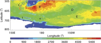
Figure 1 shows the major topographic features in the Ross Sea sector taken from GEBCO (www.ngdc.noaa.gov/mgg/gebco, accessed January 2009). The structure of the Ross Sea gyral system is not likely to be independent of the ACC, hence the domain goes from the bathymetric platform south of New Zealand (Campbell Plateau (A) in Fig. 1) to the Antarctic continent. The ACC in this sector typically crosses Macquarie Ridge (C) from west to east, and is then steered by Campbell Plateau into the south-western Pacific Basin (B). The Pacific-Antarctic Ridge (D) appears to act as a southern boundary (SB) for the ACC in this sector, separating it from the gyral system to the south. The topographic steering of the ACC has long been noted (e.g. Gordon et al. Reference Gordon, Molinelli and Baker1978), and the synthesis of observations by Orsi et al. (Reference Orsi, Whitworth and Nowlin1995) suggests how the southern boundary of the ACC lies around the entire continent (see, in particular, their figs 3, 7 & 15).

Fig. 1

Bathymetry in metres for the Ross Sea sector. Topographic features are: A. Campbell Plateau, B. south-western Pacific Basin, C. Macquarie Ridge, D. Pacific-Antarctic Ridge, E. south-east Pacific Basin, and F. the Ross Sea and the Antarctic continental shelf. Smaller features are: 1. Auckland Island, 2. Campbell Island, 3. Balleny Islands; and 4. Scott Island (not resolved) and seamounts.

Along the Antarctic coastline in Fig. 1 the Ross Sea continental shelf (F) acts as a southern boundary to the gyral system. To the east, there is the deep expanse of the south-east Pacific Basin (E). To the west, there is the extension of the Pacific-Antarctic Ridge, including surface and near-surface expression from the Balleny Islands (3) and Scott Island (not resolved at this scale) and Scott Seamounts (4). As we shall show later, these small-scale features seem to impact model representation of part of the Ross Sea gyral system.

There are particular currents on the landward side of the Antarctic gyres associated with water mass transitions from the deep water to the continental shelf, and also flows actually on the shelf (e.g. Jacobs Reference Jacobs1991, Whitworth et al. Reference Whitworth, Orsi, Kim, Nowlin and Locarnini1998). The water mass transition is between off-shelf Modified Circumpolar Deep Water (MCDW) and Antarctic Surface Water (AASW). This (horizontal) transition locates the Antarctic Slope Front (ASF) and its associated current, the ASF current (ASFC). Situations arise in which the AASW lies above water formed on the shelf with density similar to that of the MCDW. In this case the density surfaces form a characteristic inflection (or ‘V’ shape), with the ASF and ASFC associated with the off-shore part of the ‘V’. On the shelf can be found the Antarctic Coastal Current. Heywood et al. (Reference Heywood, Garabato, Stevens and Muench2004) studied the ASFC and Antarctic Coastal Current for the Weddell Front and noted that it is not always possible to clearly separate these two currents, especially where the continental shelf narrows. The Ross Sea shelf is relatively broad, allowing for identification of both components.

Recent modelling by Assmann & Timmermann (Reference Assmann and Timmermann2005) notes that the Ross Sea gyre “transport and structure are largely unknown except for a few estimates (e.g. Locarnini Reference Locarnini1994, Gouretski Reference Gouretski1999)”. Their model has a horizontal spatial resolution of 1.5° in longitude and 1.5° cos(φ) in latitude (where ϕ is the latitude). In their fig. 2 the model has a main gyre centred around 155°W, and circulating some 20 Sv (1 Sv = 1 x 10⁶ m³ s^-1). Their model also shows a gyre further to the east of the main gyre centred about 105°W, 67°S, and recycling some 9 Sv; this eastern “Ross Gyre extension” is effectively bounded to the east by the Antarctic Peninsula, in line with inferences by Locarnini (Reference Locarnini1994). As noted by Assmann & Timmermann (Reference Assmann and Timmermann2005), observations also suggest that the eastern boundary could lie between 125°W (as found by Reid Reference Reid1986 and Botnikov & Chuguy Reference Botnikov and Chuguy1989) to perhaps 140°W (as in Locarnini Reference Locarnini1994, Gouretski Reference Gouretski1999).

Fig. 2

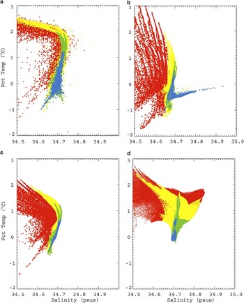
Θ-S scatter plot for a. WOCE Southern Ocean database output, b. HadGEM1.1, c. HiGEM1.1, and d. BRAN2.1 for bottom depths > 2000 m for output below 300 m. Red, yellow, green, and blue points are for depths 300–1000, 1000–2000, 2000–3000, and 3000 m to the bottom, respectively. Below 2000 m BRAN2.1 restores to climatology using an annual time scale.

Another estimate comes from an inverse model calculation by Chu & Fan (Reference Chu and Fan2007), in which hydrographic and surface wind data are combined using geostrophic balance in order to obtain a transport streamfunction on a regular 1° global grid. A reconstruction of (January) Ross Sea circulation is shown in their fig. 8, with a single eastern gyre centred around 155°W, 67°S, with transport between 15–30 Sv, and an eastern boundary between 150–140°W.

In a broader study, Wang & Meredith (Reference Wang and Meredith2008) examined the nature of the southern subpolar gyres in a number of global coupled climate models. For their Ross Gyre, they measured the gyre strength in terms of the maximum westward transport across 150°W. For the 20 models examined the estimated transports ranged from 0.1–52.0 Sv, with HadGEM1 (Johns et al. Reference Johns, Durman, Banks, Roberts, McLaren, Ridley, Senior, Williams, Jones, Rickard, Cusack, Ingram, Crucifix, Sexton, Joshi, Dong, Spencer, Hill, Gregory, Keen, Pardaens, Lowe, Bodas-Salcedo, Stark and Searl2006, the IPCC counterpart to HadGEM1.1) having 26.8 Sv. They noted that the transport estimate by Gouretski (Reference Gouretski1999) of 8.5 Sv is perhaps an underestimate of the strength of this gyre as Gouretski’s calculation neglected the depth-averaged (barotropic) component of the flow.

Wang & Meredith (Reference Wang and Meredith2008) noted that the model Ross gyres typically fill the Ross Sea, with an eastern boundary around 140°W, consistent with Gouretski’s (Reference Gouretski1999) analysis of hydrographic data. Some models do extend this eastern boundary toward the Antarctic Peninsula, however, only one of the 20 models suggests significant westward circulation this far to the east. To the west, the model solutions are more variable, with some suggesting flow extending into the neighbouring Australian-Antarctic basin. In summary, Wang & Meredith (Reference Wang and Meredith2008) observe that “there are considerable discrepancies in the simulated gyre strengths and structures”.

From observational data, Orsi et al. (Reference Orsi, Whitworth and Nowlin1995) show in their fig. 7 the SB of the ACC (and by implication the boundaries of the Antarctic gyral systems). To the west of the Ross Sea between 145°–175°E there is a northwards turn of the ACC, consistent with Reid & Mantyla (Reference Reid and Mantyla1971) and Locarnini (Reference Locarnini1994) who infer cyclonic circulation to the north of the Balleny Islands (labelled 3 in Fig. 1) associated with a western Ross Gyre. To the east, the SB turns south at 140°W and then approaches the continental shelf around 100°W before being deflected northwards further to the east by the Antarctic Peninsula.

The models

Two of the models used in this work are fully coupled global Atmosphere-Ocean-Sea-ice General Circulation Models (AOGCM) called HadGEM1.1 and HiGEM1.1, which are configurations of the Met Office Unified Model. To get a model representation of present day climate a “spin-up” is performed in which the model is run over many forcing cycles (typically as many cycles as permitted by the available computing resources) in order to arrive at a balanced state dependent on the initial conditions and the applied forcing; this balanced state is referred to as the “control”. From a decade of this control period monthly mean outputs have been compiled. HadGEM1.1 is a modified version of the HadGEM1 configuration described fully by Johns et al. (Reference Johns, Durman, Banks, Roberts, McLaren, Ridley, Senior, Williams, Jones, Rickard, Cusack, Ingram, Crucifix, Sexton, Joshi, Dong, Spencer, Hill, Gregory, Keen, Pardaens, Lowe, Bodas-Salcedo, Stark and Searl2006). Relevant changes to HadGEM1.1 are improved coupling between atmosphere and ocean (including enabling the coupling of ocean currents to the atmosphere model), with further modifications to atmospheric filtering, sea ice albedo, and other coupled model elements. Roberts et al. (Reference Roberts, Clayton, Demory, Donners, Vidale, Norton, Shaffrey, Stevens, Stevens, Wood and Slingo2009) provide more detail on the global HadGEM1.1 control run. Spatially, the ocean component is on a regular 1° longitude-latitude horizontal grid (except for a zone near the equator where the latitude scale reduces gradually to around 1/3°). In the vertical the model is discretised onto 40 z-levels distributed between the surface and a bottom depth of 5500 m.

HiGEM1.1 builds on HadGEM1.1, but seeks to examine the impact of improved resolution in the model components on the simulated climate. HiGEM1.1 is an early version from the high resolution suite of the UK-HiGEM project as described by Shaffrey et al. (Reference Shaffrey, Stevens, Norton, Roberts, Vidale, Harle, Jrrar, Stevens, Woodage, Demory, Donners, Clark, Clayton, Cole, Wilson, Connolley, Davies, Iwi, Johns, King, New, Slingo, Slingo, Steenman-Clark and Martin2009), and specific details are provided by Roberts et al. (Reference Roberts, Clayton, Demory, Donners, Vidale, Norton, Shaffrey, Stevens, Stevens, Wood and Slingo2009). Of most relevance here is the improved regular 1/3° longitude-latitude horizontal grid resolution in the ocean and sea ice components. The vertical grid is basically that of HadGEM1.1, except for a slight spacing adjustment to reduce deep ocean grid spacings. HiGEM1.1 also has an increased atmosphere resolution of N144 (c. 90 km) compared to N96 (c. 150 km) for HadGEM1.1.

Neither of these models include ice shelves or the ocean cavities underneath (and so no representation of icebergs calving off ice shelves), and runoff draining into inland basins is lost. The models maintain the global annual mean freshwater budget via a compensating constant freshwater flux applied to the global ocean (Johns et al. Reference Johns, Durman, Banks, Roberts, McLaren, Ridley, Senior, Williams, Jones, Rickard, Cusack, Ingram, Crucifix, Sexton, Joshi, Dong, Spencer, Hill, Gregory, Keen, Pardaens, Lowe, Bodas-Salcedo, Stark and Searl2006).

The Bluelink model generates an oceanic reanalysis dataset (BRAN) using data assimilation in a multi-year ocean model integration. The system and ocean model component are described in Oke et al. (Reference Oke, Brassington, Griffin and Schiller2008). Below 2000 m the model is relaxed with a year long time scale to CARS2000 (Ridgway et al. Reference Ridgway, Dunn and Wilkin2002, 30–200°E, 70°S–0°N) blended with World Ocean Atlas 2001 (Boyer et al. Reference Boyer, Stephens, Antonov, Conkright, Locarnini, O’Brien and Garcia2002, Stephens et al. Reference Stephens, Antonov, Boyer, Conkright, Locarnini, O’Brien and Garcia2002) using a tanh profile with a length scale of 2.5°. Daily means are accessible, but for the model comparison here only the long-term monthly means are analysed. As the system has evolved, the reanalyses have been updated. For this study BRAN2.1 has been used, covering the period from late 1992 to the end of 2006.

The Bluelink system does not include components other than ocean (so no sea ice or ice shelves), and as such limits itself to a lower latitude of 75°S. A conservative sea ice masking mimics the presence of sea ice by setting heat fluxes to zero in each cell where the temperature falls below -1.8°C. Despite limited representation of Ross Sea processes Bluelink has advantages in terms of resolution with a 1/10° regular horizontal longitude-latitude grid for 90–180°E and south of 17°N, slowly increasing to 0.9° in longitude by 190°E and then constant at 0.9° out to 10°E. In the vertical the Bluelink ocean model has 47 z-levels, but with the majority of these levels focussed on the upper 2000 m of the water column.

HadGEM1.1 and HiGEM1.1 have very similar vertical grid structures, with relatively regular widths over upper and deeper layers, with a gradual cell thickening over mid-depths. On the other hand the BRAN2.1 vertical grid is relatively strongly compressed over the top 2000 m, with sparser allocation down to around 5000 m.

Ross Sea sector off-shelf circulation

Figure 2b–d shows mean potential temperature (Θ) against salinity (S) for each model for summer (here December–March, inclusive) for the deep off-shelf waters, and Fig. 2a shows the observations taken from the World Ocean Circulation Experiment (WOCE) Southern Ocean Atlas database (http://woceSOatlas.tamu.edu, accessed December 2009) and is comparable to fig. 5b in Gouretski (Reference Gouretski1999). The climate models in Fig. 2b & c recover the turning point shown by Gouretski (Reference Gouretski1999) and Fig. 2a for S ≈ 34.7, but with Θ ≈ 1°C a little lower than observed. These models also have the deeper water (in green and blue) extending at an angle toward lower Θ and S in contrast to the near vertical extension in the observations in Fig. 2a. The coarser HadGEM1.1 in Fig. 2b has a broader scatter to its distribution relative to HiGEM1.1 in Fig. 2c, and HadGEM1.1 also has a set of deeper points extending out toward high salinity, not seen in observations or HiGEM1.1, and might be due to the coarser model resolution and its generation of deep water over the steep continental slopes.

As we shall show later, BRAN2.1 does not produce bottom water on the shelf. However, the model (weakly) restores to climatology below 2000 m. This is the likely explanation for why in Fig. 2d, BRAN2.1 locates the observed turning point in about the right place (Θ ≈ 1.5°C, S ≈ 34.75), with a near vertical extension for the deeper waters consistent with the observations. However, the model also generates a significant wedge of warmer and saltier water, suggesting that the deep restoring is not able to compensate for all missing processes at these latitudes.

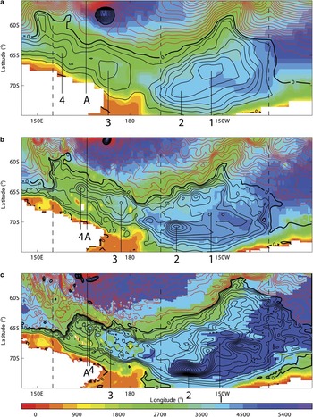
Model large-scale circulation features in the Ross Sea sector are shown in terms of derived streamfunctions in Fig. 3. These approximate streamfunctions have been derived from the depth integrated model transport components by an iterative integration across the spatial domain. This process finds a best-fit streamfunction consistent with actual transport values. This is approximate in that the iteration returns an error estimate (typically a few percent of maximum values) and because these models each use a free-surface formulation. The streamfunction is nevertheless useful for visualisation, but note that transport across sections (see later) is calculated from the actual depth integrated flows. For a discussion on streamfunctions and free surface models see appendix F in Dukowicz & Smith (Reference Dukowicz and Smith1994).

Fig. 3

Colour contours of model bathymetry (m, colour bar) overlaid with decadally-averaged streamfunction contours (Sv) for a. HadGEM1.1, b. HiGEM1.1, and c. BRAN2.1. Streamfunction contour intervals are a. 4 Sv (black, cyclonic circulation), and b. -8 Sv (red, anticyclonic circulation). Sections labelled 1, 2, 3, 4, and A are used for relevant transport estimates, and dashed lines locate sections for comparison with WOCE data (see text).

These streamfunctions are plotted on top of colour contours of the respective model bathymetry. In each part of Fig. 3 the gyral circulation features (cyclonic, typically) are contoured in black at 4 Sv intervals, and the larger magnitude streamfunction gradients (anticyclonic, typically) are contoured in red across the wider ACC at -8 Sv intervals. The vertical lines (labelled 1–4 and A) show where total zonal transport between the Antarctic coast and the end of each line is calculated. Lines 2–4 are associated with quasi-permanent eddy features identified in the monthly mean reconstructions. Line 1 locates the approximate eddy centre of the eastern gyre. Line A is used to estimate the model ACC transport in this sector, and extends northwards to the edge of the bathymetric platform to the south of New Zealand. Locations of vertical hydrographic sections described later are indicated by the dashed lines.

In each part of Fig. 3 there are cyclonic features within the ACC, particularly around 165–170°E and above 60°S. These features are associated with bathymetric steering of the ACC by Campbell Plateau (A in Fig. 1). In HadGEM1.1 in Fig. 3a, this quasi-permanent feature is particularly large, circulating about 40–50 Sv. It is also in HiGEM1.1, but shifted to the north-east, and recirculating some 28 Sv. In BRAN2.1, however, the quasi-permanent feature is replaced by a series of residual eddies all of smaller magnitude, and more widely distributed. The largest pair furthest north are still driven by the ACC interaction with bathymetry, but now recirculate about 12 (the western eddy) to 24 (the eastern eddy) Sv. Unlike HadGEM1.1 and HiGEM1.1, the monthly mean eddies in BRAN2.1 do not always appear in the same location, and hence these annual means are “residual” rather than quasi-permanent. These quasi-permanent eddies seem to be model artefacts associated with particular physics or resolution underpinning the Met Office Hadley Centre climate models. As far as we are aware, there is no observational evidence to suggest the existence of such eddies.

Figure 3 also shows that the long-term mean eddy structure refines as the model resolution increases from HadGEM1.1 to BRAN2.1. This is clear not only within the gyres in the Ross Sea, but also in the ACC itself. Nevertheless, the larger scale picture of Ross Sea gyres bounded by the ACC is evident in all the models.

The change in model resolution also allows better realisation of the topographic features in Fig. 1. The coarsest grid of HadGEM1.1 allows for the major features, but misses the finer scale islands and seamounts (features 3 & 4 in Fig. 1). This omission appears to allow the western gyre to span the space between the Pacific-Antarctic Ridge and the continental shelf. In contrast, as the resolution increases from HiGEM1.1 to BRAN2.1, the increased topographic complexity seems to both confine and complicate the structure of this part of the gyre. Indeed, the westernmost end of the gyral system can be seen in terms of a northwards diversion of the wider ACC flows, and then turning to the east as the northern edge of the gyre forms. Orsi et al. (Reference Orsi, Whitworth and Nowlin1995) note that this northward turn is consistent with “the descriptions by Reid & Mantyla (Reference Reid and Mantyla1971) and Locarnini (Reference Locarnini1994), who speculate on the existence of a closed cyclonic cell to the north of the Balleny Islands (163°E) as part of the western Ross Gyre”. In HadGEM1.1 this diversion occurs around 150°E, with the ACC going east again at around 57°S and a countercurrent system lying between the Antarctic continent along 67°S and 62°S. For HiGEM1.1, this is all shifted to the east and compressed in scale north–south such that the end is around 155°E, with the north–south range from 64–60°S. BRAN2.1 shifts this western end further east again to around 155°E, and compresses the range down to 62–65°S.

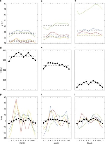
Figure 4 shows decadally averaged monthly means across the sections in Fig. 3 for HadGEM1.1 (left column), HiGEM1.1 (middle), and BRAN2.1 (right column), respectively. In each column the top part of the figure plots the monthly total westward transport across sections 1 (blue), 2 (green), 3 (orange), and 4 (red), the middle part the monthly total eastward transport across section A (•), and the bottom part their respective percentage anomalies per month. The aim is to see if there are any consistent seasonal signals in the models, and if any changes in the wider ACC transport (here represented by the total transport across section A) impacts on the transport within the Ross Sea sector.

Fig. 4

Monthly mean transports from HadGEM1.1 (left column), HiGEM1.1 (middle), and BRAN2.1 (right). a.–c. shows plot of net westward transport (Sv) across sections 1 (blue), 2 (green), 3 (orange), and 4 (red) for each model, d.–f. shows plot of net eastward transport (Sv) across section A, and g.–i. shows plot of percentage anomaly changes for sections in parts a–c. Horizontal dashed lines in top two rows locate respective annual mean values, whereas in bottom row the dashed lines locate zero percentage change.

From Fig. 4d–f it is clear that the ACC transport reduces going from HadGEM1.1 to BRAN2.1. The increasing resolution is a likely factor, but the limited Antarctic physics in BRAN2.1 is presumably being compensated by data assimilation. The change from HadGEM1.1 to HiGEM1.1 in terms of resolution is perhaps more interesting, but again not conclusive.

The second clear signal is that the ACC transport in each model, Fig. 4d–f, has lower eastward transport in the summer months (typically November–February) relative to the annual mean (shown as the horizontal dashed line). The remaining months typically have transport above the mean, except for HadGEM1.1 and BRAN2.1 which each show a clear dip in June and July, respectively. This pattern of model response has been noted before by Hughes et al. (Reference Hughes, Meredith and Heywood1999) in the Fine Resolution Antarctic Model (FRAM, FRAM Group 1991), a model similar to those studied here, but with a spatial resolution of 0.5° in longitude by 0.25° in latitude. In particular, in figs 6 & 7 in Hughes et al. (Reference Hughes, Meredith and Heywood1999) total ACC transport across Drake Passage is plotted for monthly means from FRAM, showing transport below the mean from November–February, above average transport for March–April and September–October, and near average transport from May–July. The correspondence to the present set of models is clear, especially the dip in transport in the middle of the year in HadGEM1.1 and BRAN2.1.

Hughes et al. (Reference Hughes, Meredith and Heywood1999) find a strong correlation between circumpolar transport and wind stress, both in the model and in observational datasets comprising bottom pressure measurements in Drake Passage and meteorological wind stress analyses. In particular, they conclude that wind stress to the south of Drake Passage can explain most of the wind stress and transport correspondence. This is their so-called “Southern Mode” of variability, described in terms of topographically modified barotropic Rossby waves. This mechanism is explored in Olbers & Lettmann (Reference Olbers and Lettmann2007) for the ACC, where fast and slow adjustment time scales are considered in terms of barotropic and baroclinic Rossby waves. Note, however, that Böning et al. (Reference Böning, Dispert, Visbeck, Rintoul and Schwarzkopf2008) conclude that decadal changes in wind stress do not impact the ACC transport.

The model seasonal fluctuations in ACC transport are also similar to those associated with the semi-annual oscillation (SAO), e.g. see fig. 8 in Bromwich & Wang (Reference Bromwich and Wang2008) for zonally averaged mean sea level pressure between 60–70°S showing observed lows in April and October, between January and June highs. During these lows, the westerlies increase, and it may be that model representation of this process is leading to a consequent increase in the ACC transport (presumably with a barotropic time scale). Climate models are known to simulate the SAO (see Raphael & Holland Reference Raphael and Holland2006), albeit with too small a spring peak, and so it is likely that the present climate models continue that trend. Further, BRAN2.1 is forced with reanalysis winds. A fuller analysis is outside the scope of the present paper, but it would be interesting to look more closely at the model responses, and to consider why HiGEM1.1 does not have the ACC transport dip around the middle of the year.

The model gyral transports in Fig. 4a–c suggest some response to variations in ACC transports, especially for reductions during the summer. The correspondence is most apparent for the western sections 3 and 4 in each model, whereas there is a more varied response across the models in terms of the eastern gyral sections 1 and 2. In terms of the percentage changes relative to the annual means in Fig. 4g–i, it is clear that significant variability in gyral transport arises across the seasons, with the largest ranges of between -30 to 40% anomalies for HadGEM1.1, down to around -15 to 15% for BRAN2.1. Ascribing causality to these fluctuations in the context of long-term means is not possible, but the models do suggest a number of time scales are involved in the interplay between the ACC and the gyral system.

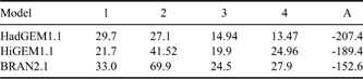
The long-term mean transports across each section are given in Table I for each model. The most notable feature is that as the ACC transport (here measured across section A) reduces as the model resolution increases (from HadGEM1.1 through HiGEM1.1 to BRAN2.1) the transports across sections 2–4 increase. However, section 1 at the centre of the eastern gyre is slightly lower in HiGEM1.1 relative to the other models. The largest change is in the transport across section 2 which grows strongly from HadGEM1.1 to BRAN2.1. This is associated with a specific quasi-permanent eddy within the wider eastern gyre. Given that the model forcings and physics are model dependent, resolution is unlikely to be the only factor of importance; even within this small sub-set of models the Ross Sea circulation remains highly variable.

Table I

Long-term mean westward transport (Sv) across sections 1, 2, 3, 4, and A for HadGEM1.1, HiGEM1.1, and BRAN2.1 as shown in Fig. 3.

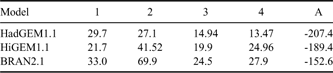
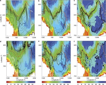
Figure 5 presents a view of these gyres in terms of water masses. Here we use the neutral density (Jackett & MacDougall Reference Jackett and MacDougall1997) surfaces γⁿ of 28 and 28.27 kg m^-3 as boundaries between the lighter AASW, the intermediate CDW, and the densest Shelf Water or Antarctic Bottom Water (AABW). These are the delineations used by Orsi et al. (Reference Orsi, Johnson and Bullister1999), Rintoul et al. (Reference Rintoul, Hughes and Olbers2001) and Orsi & Wiederwohl (Reference Orsi and Wiederwohl2009) in discussing water mass properties both on and off the Ross Sea shelf. In each part of the figure the colour contour is bathymetry (hm, the colour bar), the red dots are the SB from Orsi et al. (Reference Orsi, Whitworth and Nowlin1995), the orange contour is the 0 Sv transport streamline, and the black and white contours are the depths of the respective γⁿ surfaces (γⁿ = 28 kg m^-3 for the top row, γⁿ = 28.27 kg m^-3 for the bottom). The models HadGEM1.1, HiGEM1.1 and BRAN2.1 are in the left, middle, and right columns, respectively. Recall that below 2000 m BRAN2.1 restores to climatology using an annual time scale.

Fig. 5

Colour contours of bathymetry (hm, colour bar) with overlaid black and white contours of γⁿ depths (m) for top row γⁿ = 28 kg m^-3, and bottom row γⁿ = 28.27 kg m^-3 for a. & d. HadGEM1.1, b. & e. HiGEM1.1, and c. & f. BRAN2.1. For top row white contour intervals (CI) are 400 m, black CI are 40 m, and for bottom row black CI are 200 m and white CI are 40 m. Red dots locate ACC southern boundary from Orsi et al. (Reference Orsi, Whitworth and Nowlin1995). Orange curve locates 0 Sv contour for each respective model streamfunction. Below 2000 m BRAN2.1 restores to climatology using an annual time scale.

For the top row, the shallowing of the density surface (measured by contours around depths of 200 m) matches closely the 0 Sv streamline going east to around 150°W, the northernmost extent of the eastern gyres. As the flow turns to the south, the density contours now start to separate from the 0 Sv line, and that separation widens as the coastline is approached and the gyre now circulates to the west. Going from HadGEM1.1 (Fig. 5a) to BRAN2.1 (Fig. 5c) the distance between the coast and the density contour at 200 m narrows considerably. All the models show the density surfaces doming toward the centre of each gyre. In terms of matching the SB from Orsi et al. (Reference Orsi, Whitworth and Nowlin1995) the γⁿ = 28 kg m^-3 surface provides a remarkably good match for BRAN2.1, apart from the initial northward diversion at around 150°E. In contrast HadGEM1.1 and HiGEM1.1 only follow the SB closely along the ridgeline to the north. At the western end of the gyral system these models have too northward an excursion. At the eastern end the density surfaces tend to lie too far to the west of the SB, but the model 0 Sv lines provide for a reasonably close match.

The lower row of Fig. 5 can be compared with fig. 6 in Orsi et al. (Reference Orsi, Johnson and Bullister1999) showing the depth of the γⁿ = 28.27 kg m^-3 surface. For HiGEM1.1 in Fig. 5e the eastern gyre structure is well represented, apart from perhaps the density surface depths being a little shallower than observed. The surface shallowing into the western gyral system is picked out, as well as the deepening again further to the west. For HadGEM1.1 in Fig. 5d, the eastern gyre is also clear, but all the depths are shallower than both observed and HiGEM1.1. The surface shallows over the western gyral system, but again too much and the isosurfaces are more regular than in the other models. The HadGEM1.1 surfaces deepen to the west. BRAN2.1 in Fig. 5f reproduces the layer depths well for the eastern gyre (apart from an overly shallow layer mid-gyre as evidenced by the white contours) and captures the shallowing over the western gyral system, and then the deepening further west. Note that the climate models have white contours over the shelf and slope showing the production of deep water not captured by BRAN2.1. Clearly the ability of BRAN2.1 to maintain aspects of the deep water structure is associated with the restoration to climatology on annual time scales below 2000 m.

Fig. 6

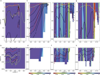
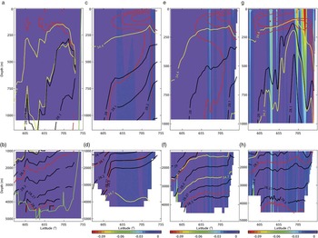
Red, yellow, and black line contours of potential temperature (at -1, 0, 1°C), salinity (at 34.4 and 34.7), and γⁿ (at 28, 28.1, 28.2, 28.27, and 28.3 kg m^-3), respectively, along 155°E for a. & b. WOCE section P11, c. & d. HadGEM1.1, e. & f. HiGEM1.1, and g. & h. BRAN2.1. Background colour contour for c–h, inclusive, is respective model zonal flow (m s^-1, colour bar), the scale chosen to highlight negative (westward) zonal flow component. Background colour for a & b is for plotting consistency and has no flow significance. Upper row shows top 1000 m, bottom row 1000 m to the bottom. Green contour on a & b is reference bathymetry from GEBCO.

Orsi et al. (Reference Orsi, Johnson and Bullister1999) also show bottom layer averaged contours for Θ and S (their fig. 7b & c, respectively). HiGEM1.1 average Θ reproduces the observed east–west gradient quite well. On the other hand, the deep water in HadGEM1.1 is on average colder and saltier than either HiGEM1.1 or the observations. BRAN2.1 captures the observed pool of Θ < 0°C water in Orsi et al. (Reference Orsi, Johnson and Bullister1999) for the eastern gyre quite well, but like HadGEM1.1 the bottom layer tends to be too saline.

Fig. 7

Red, yellow, and black line contours of Θ, S, and γⁿ, respectively along 170°W for a. & b. WOCE section P15, c. & d. HadGEM1.1, e. & f. HiGEM1.1, and g. & h. BRAN2.1. Background colour contour for c–h, inclusive, is respective model zonal flow (m s^-1, colour bar), the scale chosen to highlight negative (westward) zonal flow component. Background colour for a & b is for plotting consistency only. Details as in caption to Fig. 6.

To further highlight the model differences, Figs 6–8 show cross sections at 155°E, 170°W, and 135°W, respectively, for comparison with the equivalent sections P11, P15, and P17 in the WOCE Southern Ocean Atlas (Orsi & Whitworth Reference Orsi and Whitworth2005). These sections are shown as dashed lines in Fig. 3. In each figure the black, red, and yellow contours highlight Θ, S, and γⁿ, respectively, for (from left to right) the relevant WOCE section, HadGEM1.1, HiGEM1.1, and BRAN2.1, and the background colour shows zonal speed for the models (but is for colour consistency only for the WOCE sections). The values chosen for the black, red, and yellow contours illustrate the AASW (the Θ contours, and the S = 34.4 contour), the Upper CDW (UCDW, between the S = 34.4 and the S = 34.7 contour), and the lighter to heavier water mass transitions via γⁿ = 28, 28.1, 28.2, 28.27, 28.3 kg m^-3 contours. These values are those indicated by Orsi et al. (Reference Orsi, Whitworth and Nowlin1995) in identifying the SB in terms of termination of UCDW as it shallows toward the continental shelf, and a transition from the relatively warmer ACC waters to the colder continental shelf waters. The sections in Orsi & Whitworth (Reference Orsi and Whitworth2005) typically show UCDW rising to the surface (to within a couple of hundred metres), with the colder shelf water overlying it. As a result the γⁿ = 28 kg m^-3 surface shallows and then levels off. It is these characteristic signatures that Orsi et al. (Reference Orsi, Whitworth and Nowlin1995) associated with the SB.

Fig. 8

Red, yellow, and black line contours of Θ, S, and γⁿ, respectively along 135°W for a. & b. WOCE section P15, c. & d. HadGEM1.1, e. & f. HiGEM1.1, and g. & h. BRAN2.1. Background colour contour for c–h, inclusive, is respective model zonal flow (m s^-1, colour bar), the scale chosen to highlight negative (westward) zonal flow component. Background colour for a & b is for plotting consistency only. Details as in caption to Fig. 6.

In Fig. 6 each of the models have UCDW that is typically too fresh relative to the observations in Fig. 6a. In particular HadGEM1.1 does not have a characteristic S = 34.7 contour here, and HiGEM1.1 and BRAN2.1 only have such salinities below 1000 m or so. All the models have the surface layer of AASW extending out from the coastline, with the S = 34.4 contour (characterizing the upper limit of UCDW) shallowing into this surface layer. HadGEM1.1 tends to have too much cold water over depth (compare the Θ = 0°C contours), and there is too much dense water at depth (compare the γⁿ = 28.27 kg m^-3 contours) relative to the other models and observed. However, HadGEM1.1 still has γⁿ surfaces shallowing indicating the transition from the wider ACC to the gyral system, and the isosurfaces can be seen slightly dipping toward the coastline associated with the surface intensified westward flow, and westward flow extending to the bottom. This pattern is repeated in the other models, but with increasing resolution the models are able to separate out the sloping isopycnals at the coastline associated with a surface intensified current right at the coast, and a current at the shelf break extending to the bottom. Note that in HiGEM1.1 the densest γⁿ contours actually deepen away from the coastline, and later this is shown to be AABW flowing off the shelf. In contrast, BRAN2.1 does not produce this water, and has the isolines generally dipping into the bathymetry. Nevertheless, both these models suggest a current at the coast, and another deep current at the shelf break. Finally, BRAN2.1 does not shallow the γⁿ = 28 kg m^-3 as much as the other models or as observed for this section.

Along 170°W in Fig. 7 the climate models again suggest too fresh a layer of UCDW with the S = 34.7 only apparent at depth, whereas BRAN2.1 actually captures this water mass feature for this longitude. The γⁿ = 28 kg m^-3 contour in each model is similar, consistent with the WOCE section and the contours in Fig. 5. Again HadGEM1.1 has too much dense water at depth relative to observations. All of the models have a dip in the isosurfaces as the shelf break is approached but, because of the clear signature of deep water formation on the shelf in the climate models, the deeper isolines slope back up again toward the coastline and onto the shelf. The isosurface dip around 67°S is hinted at in the WOCE section, however, the section presently terminates around this latitude, so no direct confirmation of the model behaviour closer to the coast is possible.

For 135°W in Fig. 8 the climate models again underestimate the salinity of the UCDW water relative to the observations and BRAN2.1. At this end of the shelf, each of the models seems to be doing a better job of capturing the density structure seen in the observations. Indeed, BRAN2.1 reproduces quite well the shallowing of the γⁿ = 28 kg m^-3 surface and its subsequent dip toward the coastline, and presumably contributes to the more consistent SB location found here in BRAN2.1 (see Fig. 5).

Comparison with float data

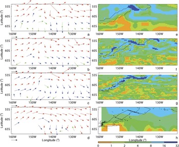
From an analysis of autonomous float data, Davis (Reference Davis2005) presents average velocities at 900 m depth across the Pacific Ocean. The floats analysed by Davis (Reference Davis2005) “park” at around 900 m as part of their duty cycle. Analysis of their positions when they report at the surface enables an estimate of the flow at 900 m to be built up. It is that flow we consider here. Of particular interest are figs 10 & 12 in Davis (Reference Davis2005), as some of the floats manage to sample the northern boundary of the Ross Sea sector. The relevant vectors have been scanned in from Davis (Reference Davis2005), and are reproduced in Fig. 9d. Although the analysis is on a relatively coarse grid (about 300 km spatial resolution), flow south from the ACC toward the eastern end of the sector between about 145–135°W is apparent, as are flow magnitudes in this region of between 3–9 cm s^-1. Also evident is the general cyclonic sweep of the ACC (with average peak speeds around 10 cm s^-1) to the north of the sector, with eastward turning to south-eastward flow toward the eastern end of the sector between 130–120°W. As Davis (Reference Davis2005) notes, there are insufficient observations in the Southern Ocean to detail flow south of the ACC “except southward flow into the Ross Sea near 65°S, 140°W″.

Fig. 9

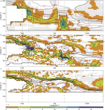
Long-term average velocity vectors (averaged onto regular 3° grid) and speeds (cm s^-1, interpolated to HiGEM1.1 grid) of model output for a. & e. HadGEM1.1 at 874 m, b. & f. HiGEM1.1 at 963 m, and c. & g. BRAN2.1 at 995 m, respectively. d. & h. show mean autonomous float velocity vectors at 900 m scanned in from Fig. 12 in Davis (Reference Davis2005) and their inferred speeds, respectively. The model depths represent the nearest mid-depth cell positions to 900 m. Each vector is scaled relative to the reference vector of magnitude 1, 3, and 9 cm s^-1 for the red, blue, and green vectors, respectively. Speeds of < 1 cm s^-1 are green, between 1–3 cm s^-1 are blue, and > 3 cm s^-1 are red. Black contours are isobaths at 3000 m from the respective model (e–g) or from GEBCO (h).

Fig. 10

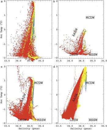
Θ-S scatter plot for a. WOCE Southern Ocean database output, b. HadGEM1.1, c. HiGEM1.1, and d. BRAN2.1 for bottom depths < 2000 m for output below 30 m. Red, yellow, green, and blue points are for depths 30–500, 500–1000, 1000–1500, and 1500 m to the bottom, respectively.

For comparison, velocity vectors from the models have been averaged onto a regular 3° grid for HadGEM1.1, HiGEM1.1, and BRAN2.1 at depths of 874 m, 963 m, and 995 m, respectively. These depths represent the nearest mid-depth cell positions to 900 m for each model. The resultant vectors are plotted in Fig. 9a–c using the colour scheme of Davis (Reference Davis2005) to highlight flows speeds of < 1 cm s^-1 (green), speeds between 1–3 cm s^-1 (blue), and those > 3 cm s^-1 (red). Flow magnitudes from the models and inferred from the Davis (Reference Davis2005) vectors are shown in Fig. 9e–h, each interpolated to the HiGEM1.1 grid for a common reference. The 3000 m isobath from the respective model and then from GEBCO has also been plotted on the flow magnitude figure parts.

Each model captures the general observed flow pattern in Fig. 9d, with the greater magnitude red vectors in the north, changing to the smaller blue and green vectors going south. The flow magnitudes in Fig. 9e–h show the same trend, but more model fine-scale structure in these long-term means is apparent going from HadGEM1.1 to BRAN2.1 resolution, reflecting the structure seen in the streamfunctions in Fig. 3. Each model also shows peak flows (> 16 cm s^-1) overlying the fracture zone shown by the bathymetric contours, and evidence of strong flows along the ridge, especially for HiGEM1.1 (Fig. 9f) and BRAN2.1 (Fig. 9g). This model sensitivity to the bathymetry is reflected in their respective vector fields as well, with a relatively sharp transition from north-east to near southward flow at these depths around 145°W, 57°S. Beyond about 130°W the models also have a more zonal flow pattern compared to the analysis in Fig. 9d, especially to the north.

Flow into the Ross Sea represented in HadGEM1.1 and BRAN2.1 in Fig. 9a & c, respectively, by a clear band of southward vectors between about 145–130°W, south of 60°S is similar to that in the float data. The flows in HiGEM1.1 in Fig. 9b in this area suggest that the southward turning is pushed further to the east and south than either of the other models or the floats imply.

Ross Sea sector on-shelf circulation

Figure 10b–d shows model Θ-S for on-shelf waters, and Fig. 10a shows observations taken from http://woceSOatlas.tamu.edu (accessed December 2009), comparable to fig. 4 in Gouretski (Reference Gouretski1999) and fig. 2 in Orsi & Wiederwohl (Reference Orsi and Wiederwohl2009). Each model captures the upper turning point at S ≈ 34.7, but the peak Θ in HadGEM1.1 (Fig. 10b) and HiGEM1.1 (Fig. 10c) of around 0°C and 1.2°C, respectively, is less than the c. 1.8°C observed and obtained by BRAN2.1 (Fig. 10d). Figure 10a and fig. 2 in Orsi & Wiederwohl (Reference Orsi and Wiederwohl2009) show that water with γⁿ > 28.27 kg m^-3 is formed on the shelf, and this is true for the climate models for their deepest waters. However this component is completely absent from BRAN2.1 since deep water formation processes on the shelf are not included. The climate models both generate High Salinity Shelf Water (HSSW) extending out toward S ≈ 35.0, but at temperatures perhaps a degree or two warmer than observed. However, as none of the models have ice shelves, the coldest observed shelf water in Fig. 10a formed by ice shelf melt is not produced.

Recent work by Park et al. (Reference Park, Gasco and Duhamel2008) has shown that estimates of depth-averaged (“barotropic”) flow velocity and hence transport can be obtained from analysis of longline fishing data, based on the assumption that the longline fishing gear drifts with the prevailing current while sinking to the seabed. When deployed a demersal longline consists of two buoys at the surface each of which locates the approximate horizontal position of weighted chain and grapnel or anchor on the bottom. The weights at the bottom are connected to their respective surface buoys by a “downline” in the vertical, and to each other in the horizontal along the bottom by the “mainline” or “backbone” to which are attached the baited hooks. The process to obtain this deployed state is referred to as the “set”. The recovery phase of this gear is the “haul”. In the set phase one of the buoys and its downline are put into the water, and this initial position recorded. The weights are then thrown into the water with the mainline attached. At this time the sink rate of the mainline is measured. At the other end of the downline more weights then follow, with again a downline and the other surface buoy. Surface movement through the water of the deploying vessel is aimed at preventing entanglement and snapping of the downline, and to enable optimal bottom coverage by the downline.

For the Ross Sea sector longlines with lengths between one and about 27 km (mean 8.5 km, with standard deviation (SD) 6.3 km) are used. Longlines are typically set on the seabed at depths 500–1900 m (mean 1160 m, SD 320 m), with fishing generally occurring between December–March each year. A total of 9909 longline fishing “events” (where an event comprises the line being “set” and then “hauled”) were recorded in the Ross Sea between 1997–2008. However, before 2002 sink rate tests were not reported, and hence only data from years 2002–08 (n = 8394) will be used.

For each event, the positions of the start and end of the line set and the haul were recorded by Convention on the Conservation of Antarctic Marine Living Resources (CCAMLR) observers. Longline gear sink rate was measured using either a time-depth recorder or a timed bottle test. Test are required to be attempted on at least one longline set every 24 hour period, and four concurrent tests every seven days on a single longline to determine any sink rate variation along the longline. Protocols for the sink rate tests are described in CCAMLR Conservation Measure 24-02 (http://www.ccamlr.org/pu/e/e_pubs/cm/drt.htm, accessed August 2009). Mean recorded sink rates were 0.42 m s^-1 (SD 0.36 m s^-1, from n = 5858 individual tests) over all vessels, years and trips in the Ross Sea. As observer data often contain reporting and transcription errors, we restricted analysis to a range of plausible values for sink rates, i.e. within the range of 0.15–0.75 m s^-1 (n = 5995). Sink rate tests were conducted on a subset of all longline fishing events by vessels in the Ross Sea (n = 2829). Sink rates for those fishing events where sink rate tests were not carried out were assumed to be the median sink rate for that vessel for that year.

It is assumed firstly that the weights sink at the same rate as that measured for the mainline. If large differences did occur between these rates then the mainline either would break, or become entangled; hence it is in the best interests of the vessel to ensure the sink rates are comparable. Secondly, the weight is assumed to drift with the depth-mean current as it traverses the surface to the bottom. Hence, for each weight it is possible to obtain the distance and direction between its initial location when thrown in and where it settles at the bottom. Echo sounding determines the local bottom depth, and dividing that by the sink rate approximates the time to reach the bottom.

The distance between the set and haul was calculated as the difference in position between the mean of the start and end of the set, and the mean of the start and end of the haul. A depth averaged speed is then this distance divided by the time to reach the sea bed. Hence, the depth-averaged flow velocity of each fishing event was determined.

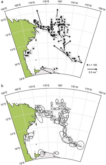
Each fishing event was then allocated to an equal area square grid within the Ross Sea approximately 21 nautical miles (38.5 km) along each edge. Fishing events occurred within 171 grid cells, but only 80 cells had more than 10 fishing events (95% of all fishing events). Within each grid cell, the mean depth-averaged flow velocity was calculated as the mean velocity of the individual fishing events within that cell. This compares to the 75 cells obtained by Park et al. (Reference Park, Gasco and Duhamel2008) with at least 80 data points and with a mean of 336 points per cell. The averaging process should largely account for biases due to strong tidal currents, however, the present sampling is undoubtedly below that of Park et al. (Reference Park, Gasco and Duhamel2008). The resultant flow from these 80 cells for the Ross Sea is shown in Fig. 11a. Despite the limitations of the longline analysis, the estimates suggest average transport on the shelf from east to west. To the east there is a northward turn at 177°W, and then flow toward Iselin Bank (at around 180°E, 72°S). Directly west of Iselin Bank the flow is indistinct, but as Cape Adare is approached at the western end of the shelf a strong consistent westward flow is seen. The inferred flow magnitudes are also significant, with speeds in excess of 50 cm s^-1 in some areas.

Fig. 11

Barotropic flows reconstructed from historical longline information. Each vector in part a is an average over each dashed square, their magnitudes relative to the reference vector of speed 0.5 m s^-1. The area of the circle in each square indicates number of independent measurements per mean relative to size of reference circle (n = 100). The standard error ellipses in part b are obtained from 1000 bootstrap samples (see text), and are drawn centred on their respective cells.

Standard errors are plotted in Fig. 11b. The standard errors of the sampling distributions of the zonal and meridional components of the drift vector were obtained for each cell using the bootstrap method (1000 bootstrap samples). The bootstrap method is a general resampling process, in which independent bootstrap samples are constructed with replacement from the original distribution, the relevant statistic (e.g. the mean) is then calculated for each bootstrap sample, and then standard errors can be found from the many (here 1000) bootstrap samples (Efron Reference Efron1979). It is an appropriate method in this context as the mean depends on the distribution of events. Ellipses are then drawn that represent the approximate standard error confidence regions for the endpoints of the mean drift vectors, with each ellipse in the figure centred on its respective cell.

Many of the ellipses show that speed errors that are a significant fraction of the mean arise, reflecting perhaps the smaller samples we have. In terms of direction, however, many ellipses are relatively narrow along the mean vector, suggesting that there is some consistency in the obtained flow directions. There is no doubting the general imprecision of this method. Indeed, Park et al. (Reference Park, Gasco and Duhamel2008) note that comparisons between in situ measured and longline-derived time mean flows at the same location show that the method has errors of 10% in speed and about 10° in direction. In our case the standard error ellipses do not invalidate the implied mean circulation, in particular general east–west flow across the shelf, northwards transport toward Iselin Bank, and then strong westward flow toward Cape Adare.

Figure 12 shows the barotropic circulation from each model for the shelf region of the Ross Sea. Each figure shows the model mean barotropic vector flow on top of flow magnitude colour contours, with red contours for the transport streamfunction and black contours for the 1000 and 3000 m isobaths. For this comparison the models have been interpolated to the HiGEM1.1 resolution, and to aid clarity, vector magnitudes less than 0.75 cm s^-1 and colour contours below 2 cm s^-1 are not shown.

Fig. 12

Barotropic flow vectors (relative to scale vector of 4 cm s^-1) for a. HadGEM1.1, b. HiGEM1.1, and c. BRAN2.1 for Ross Sea. In each red bathymetry contours at 1000 and 3000 m, black transport streamfunction contours at values of 0, 1, 2, 3, 4 and 8 Sv, and colour contours of barotropic speed (cm s^-1). Minimum magnitude for vector to be plotted is 0.75 cm s^-1, and colour contours of barotropic speed above 2 cm s^-1 only, each for clarity. Straight black contours in each part locate model land-sea boundaries, and dashed lines locate model sections.

The significant on-shelf flows in HadGEM1.1 and HiGEM1.1 in Fig. 12a & b, respectively, are consistent with the longline estimate, suggesting a general east–west circulation. The climate models show flow impinging on the shelf at around 170°W, which is then steered westwards by the lower model coastline. Both models then reveal a flow intensification as the circulation turns to the north and then west again. In HadGEM1.1 the westward flow toward Cape Adare is relatively broad and coherent, while that in HiGEM1.1 suggests two branches that then re-combine at the far western shelf end. As seen in the longline flows, both models have a coherent and strong westward flow at Cape Adare, with the peak HiGEM1.1 flow magnitude (between 20–50 cm s^-1) some two to three times greater than that in HadGEM1.1 (between 8–12 cm s^-1). In terms of transport, HadGEM1.1 has some 3 Sv carried on the shelf, compared to around 2 Sv by HiGEM1.1. The limited shelf representation in Fig. 12c for BRAN2.1 results in a relatively weaker on-shelf transport of around 1 Sv, but again reveals a general east–west flow, with intensification at Cape Adare.

Recent model runs by Padman et al. (Reference Padman, Howard, Orsi and Muench2009) of the Ross Sea shelf initialised with the Orsi & Wiederwohl (Reference Orsi and Wiederwohl2009) climatology show depth-averaged speeds in their fig. 8a. As here, flow intensification at Cape Adare is reproduced, as well as discrete strong flow pathways across the shelf and to the north along the eastern side of Iselin Bank. Padman et al. (Reference Padman, Howard, Orsi and Muench2009) also show that there are strong peak tidal flows on the shelf, particularly along the slope toward Cape Adare, where speeds of up to 80 cm s^-1 are found. So, despite the relatively poor statistics of the longline records, it is encouraging that the general pattern of flow is reproduced to a large degree by a range of models, and that the mean flow from the longline data toward Cape Adare manifests in an area of high peak tidal speeds. Further analysis with tidal flows is required to prove that our longline estimates are not being unduly biased by tidal flows where the sampling is low. Nevertheless, it remains encouraging that a degree of consistency on the depth-averaged flow is retained.

To the north of the 3000 m isobath, HiGEM1.1 and BRAN2.1 have significant westward flow parallel to the 8 Sv contour associated with the southern edges of the Ross Sea gyres evident in Fig. 3. All of the models show westward flow intensification along the coastline to the west of Cape Adare, showing evidence of interaction between the off-shelf gyral flow and that coming from the shelf itself. As the model resolution improves, the northward extent of this coastal flow reduces, but each model transports some 8 Sv to the west in this flow.

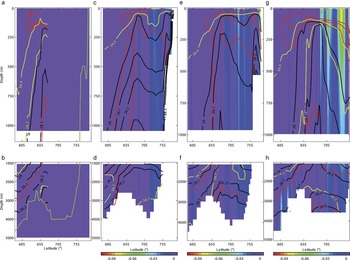
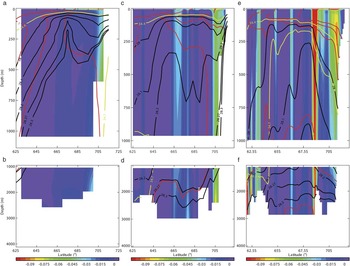
More details of the on-shelf and cross-slope flows are shown in Figs 13–15, cross sections at 170°, 172°E, and 177°W, respectively, indicated by the dashed lines in Fig. 12. Figures 14 & 15 cut through the peak depth-averaged flows on-shelf seen in the observations and models, while Fig. 13 examines the conditions just downstream off the shelf. The figures are laid out as Figs 6–8 but with a focus on the shelf and continental slope. In Fig. 13 each model has a coastal westward flow at all depths, with the peak flows at the surface. In BRAN2.1 (right-hand column) this flow is associated with isopycnals dipping down into the bathymetry. In contrast the climate models have the isopycnals closest to the coastline tilted in the opposite sense, and with the densest isolines crossing the continental slope, indicating deep water being transported off-shelf by these models. This is particularly clear in HiGEM1.1 (middle column) where the γⁿ = 28.27 and 23 kg m^-3 isopycnals fall steeply from the shelf to the ocean floor at around 2500 m, whereas HadGEM1.1 again has the densest water too high in the water column. Moving further from the shelf, the climate models also show that the upper isopycnals have a characteristic ‘V’ shape before flattening out again further north. This structure is consistent with the ASF described earlier, and indeed the zonal flows coincident with this ‘V’ may well be evidence of a model representation of an ASFC. HiGEM1.1 and BRAN2.1 also show deep zonal currents further north again, these being elements of the gyral circulation.

Fig. 13

Red, yellow, and black line contours of Θ (at -1, 0 and 1°C), S (at 34.4 and 34.7), and γⁿ (at 28, 28.1, 28.2, 28.27 and 28.3 kg m^-3), respectively, along 170°E for a. & b. HadGEM1.1, c. & d. HiGEM1.1, and e. & f. BRAN2.1. Background colour contour is respective model zonal flow (m s^-1, colour bar), the scale chosen to highlight negative (westward) zonal flow component. Upper row shows top 1000 m, bottom row 1000 m to the bottom.

Fig. 14

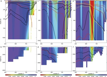
Red, yellow, and black line contours of Θ, S, and γⁿ, respectively, along 172°E for a. & b. HadGEM1.1, c. & d. HiGEM1.1, and e. & f. BRAN2.1. Background colour contour is respective model zonal flow (m s^-1, colour bar), the scale chosen to highlight negative (westward) zonal flow component. Details as in caption to Fig. 13.

Fig. 15

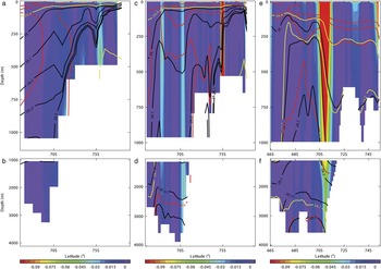
Red, yellow, and black line contours of Θ, S, and γⁿ, respectively, along 177°W for a. & b. HadGEM1.1, c. & d. HiGEM1.1, and e. & f. BRAN2.1. Background colour contour is respective model zonal flow (m s^-1, colour bar), the scale chosen to highlight negative (westward) zonal flow component. Details as in caption to Fig. 13.

Along 172°E in Fig. 14 through the fastest flows close to Cape Adare the differences between the climate models and BRAN2.1 are as equally apparent as along 170°E. Here, however, deep on-shelf flows in the climate models are clearly associated with isopycnal slopes in the lighter and densest water, with the dense water falling across shelf and then down the continental slope (particularly so in HiGEM1.1), and the upper isopycnals exhibiting the ‘V’ structures. The association of surface intensified and also deep zonal flows is clear in HiGEM1.1, where distinct flows seen in Fig. 12 are consistent with deep isopycnal slopes and separate upper ‘V’s. In HadGEM1.1 the upper isopycnals slope upward over quite a broad range of latitudes, thereby creating a wide, near surface intensified flow. In contrast, HiGEM1.1 and BRAN2.1 have a distinct isopycnal structure at around 69°S, leading to a deep zonal current at this latitude.

Figure 15 cuts through the other high speed flow on the shelf at 75°S found in the climate models. In these models this flow is again associated with isopycnal gradients, with both models showing currents reaching to the bottom driven by north–south isopycnal gradients, and both display characteristic ‘V’ shapes (particularly so HadGEM1.1 in Fig. 15a). As before, HadGEM1.1 has the densest layers perhaps too high in the water column, such that the γⁿ = 28.27 kg m^-3 isoline goes over the continental slope, but in HiGEM1.1 this remains on the shelf. At this longitude, the climate models show the continuation of many density isolines from off-shelf to on-shelf, whereas BRAN2.1 shows these typically terminating at the shelf break. At 71°S or so both HiGEM1.1 and BRAN2.1 have deep zonal flows associated with the southern boundary of their respective eastern gyres. This flow is part of the intermediate water mass structure as both models have the γⁿ = 28.27 kg m^-3 isoline down below 2500 m, and both models have isolines tilting down toward the continental shelf, but this tilt is relatively steeper in BRAN2.1 and hence leads to the stronger zonal flow.

Recent work by Orsi & Wiederwohl (Reference Orsi and Wiederwohl2009) presents an analysis of Θ and S observations on the Ross Sea shelf and over the continental slope. Their new climatology provides for distributions of water masses and their layer thicknesses, and hence for consideration of pathways for water mass transformation and redistribution in the Ross Sea. Some of those are examined in the climate models, but not for BRAN2.1 as it does not generate the relevant dense waters on the shelf.

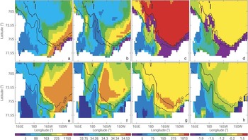
Figure 16 shows model layer thicknesses and average layer properties of Θ and S for γⁿ < 28 and 28 < γⁿ < 28.27 kg m^-3 for HiGEM1.1 (top row) and HadGEM1.1 (bottom row) for comparison with figs 5 & 7 in Orsi & Wiederwohl (Reference Orsi and Wiederwohl2009). Figure 16a & e shows the top layer thickness (L1 in Orsi & Wiederwohl Reference Orsi and Wiederwohl2009). HiGEM1.1 captures the on-shore coastal layer at the eastern end of the shelf and the thinning east–west layer gradient. However, the HiGEM1.1 horizontal spatial scales are too broad to capture the density pattern associated with the ‘V’ of the ASF along the 1000 m isobath, apart perhaps beyond Cape Adare where a broad band is found (but with greater northward extent than observed). Despite its coarser scale, HadGEM1.1 captures the observed L1 distribution well, but has no characteristic ‘V’. In terms of the average L1 salinity in Fig. 16b & f, both models have the freshest water at the western end of the shelf, but both typically underestimate the layer salinity across the shelf.

Fig. 16

Colour contours of top density layer thickness (γⁿ < 28 kg m^-3, first column) and average top layer salinity (second column) for a. & b. HiGEM1.1, and e. & f. HadGEM1.1, and for middle density layer thickness (28 < γⁿ < 28.27 kg m^-3, third column) and average layer Θ (°C, fourth column) for c. & d. HiGEM1.1, and g. & h. HadGEM1.1. Missing layer is shown by left-most (purple) colour bar. Model bathymetry at depths 1000 and 3000 m indicated by black contours.

Figure 16c & g is for the intermediate layer thickness (L2). In Fig. 16c HiGEM1.1 captures the observed east–west gradient well, and even some of the thickening out around Iselin Bank. However, at the shelf eastern end, the band of purple contours show that water of this density is not being produced here by HiGEM1.1 in contrast to observations. HadGEM1.1 in Fig. 16g also captures the L2 east–west gradient correctly, and does reproduce the coast–shelf gradient as well. Both models capture the coast–shelf gradient in Θ in Fig. 16d & h, but as expected neither model manifests the coldest waters in the observations.

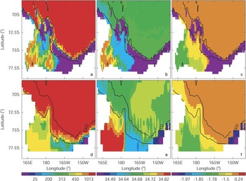
Figure 17 is for the bottom layer (L3, γⁿ > 28.27 kg m^-3) for comparison with fig. 8 in Orsi & Wiederwohl (Reference Orsi and Wiederwohl2009). As before, the top and bottom rows are for HiGEM1.1 and HadGEM1.1, respectively. HiGEM1.1’s L3 pattern starts to pick out the deep tongues seen in the observations along the troughs on the shelf remarkably well. However, the thicknesses are generally lower than seen, especially for the thickest observed at the western end of the shelf. The east–west gradients in Θ and S are captured, and the general warming from the coast out to the shelf break, but again it does not have the coldest water associated with the ice shelf. The bottom row for HadGEM1.1 has similar patterns to HiGEM1.1, but at its coarser resolution cannot capture the detail observed, and has overly saline L3 values at the western end of the shelf.

Fig. 17

Colour contours of lowest density layer thickness (γⁿ > 28.27 kg m^-3, left column), average layer S (middle), and average layer Θ (°C, right) for a.–c. HiGEM1.1, and d.–f. HadGEM1.1. Missing layer is shown by left-most (purple) colour bar. Model bathymetry at depths 1000 and 3000 m indicated by black contours.

Using these deepest layer thicknesses, it is possible to measure the AABW exported from the Ross Sea shelf in terms of the northward flux crossing the 1000 m isobath in Fig. 17 for each climate model. Using this measure, just over 4 Sv of this northward flux is found in each model. Here, the relative spatial coarseness of the models makes it problematic to use, for example, the measure of Orsi et al. (Reference Orsi, Johnson and Bullister1999) of trying to calculate the “total volume of newly-formed bottom water sinking across the 2500 m isobath of the Antarctic slope”. Here the 1000 m isobath up to 72°S for the Ross Sea effectively delineates the shelf from the slope, however, by 2500 m it becomes difficult to separate AABW formed on the shelf from that already circulating in the deep water.

Ross Sea sector sea ice

Here aspects of the sea ice representation within the Ross Sea sector are presented. The aim is to demonstrate that the models have consistent representations of the climatological sea ice distributions (at least for the coupled climate models). The related model HadGEM1 has had its global sea ice response validated and reported in McClaren et al. (Reference McClaren, Banks, Durman, Gregory, Johns, Keen, Ridley, Roberts, Lipscomb, Connolley and Laxon2006). In terms of ice area, McClaren et al. (Reference McClaren, Banks, Durman, Gregory, Johns, Keen, Ridley, Roberts, Lipscomb, Connolley and Laxon2006) report that HadGEM1’s seasonal ice area for the Southern Ocean agrees well with the observations in terms of phase, but the amplitude is too large (with annual mean ice area some 12–20% in excess of observed). In terms of thickness, HadGEM1 gives a good average in comparison to the observations. Interestingly, in comparison to its predecessor HadCM3 (Gordon et al. Reference Gordon, Cooper, Senior, Banks, Gregory, Johns, Mitchell and Wood2000), HadGEM1 produces encouragingly good estimates of the relatively low sea ice thickness in front of the Ross and Amery Ice Shelves.

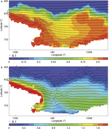
Figure 18 shows the average September distributions for HiGEM1.1 of a) sea ice concentration, and b) sea ice thickness (m) over the Ross Sea, overlaid with vectors for the surface wind stress (N m^-2) and ice velocity (m s^-1), respectively. The wind stress in Fig. 18a shows a strong offshore component coming from the continent and out over where the Ross Ice Shelf would be. To the west and along the coastline, the wind stress is closely aligned with the coast and has a relatively strong westward component. To the east, there is also evidence of a similar westward stress along the coastline but of much weaker magnitude. The offshore stress diverges in response to southward stress components further to the north along the winter ice edge, leading to predominantly eastward stress over the eastern Ross Sea sector, and mainly westward stress over the sea ice to the west.

Fig. 18

HiGEM1.1 September monthly mean colour contours of a. ice concentration, and b. thickness (m). Vector fields are September monthly means of a. surface wind stress (N m^-2), and b. ice velocity (m s^-1), each scaled to a vector magnitude of 0.1 in their respective units.

In response to the wind stress, the ice flow in Fig. 18b also has a strong northerly component in the central part of the Ross Sea sector away from where the ice shelf would be, and this is presumably responsible for the thinnest ice adjacent to the coast here. To the west, the ice flow again largely follows the wind stress, and is clearly associated with the thicker ice all along the coastline. To the east, the ice flow has a cyclonic circulation resembling the underlying Ross Sea gyre, with an offshore component near the centre, and a return coastal flow further to the east. The result is a thickening near the eastern coastline, with a tongue of ice spread out along the approximate line of the continental shelf. This is the pattern seen in HadGEM1 in McClaren et al. (Reference McClaren, Banks, Durman, Gregory, Johns, Keen, Ridley, Roberts, Lipscomb, Connolley and Laxon2006) in their fig. 7b, and reported by Assmann et al. (Reference Assmann, Hellmer and Beckmann2003) in their simulations of the Ross Sea (see their fig. 4). HadGEM1.1 produces similar distributions (not shown).

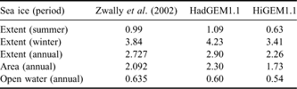
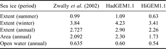
The results from Zwally et al. (Reference Zwally, Comiso, Parkinson, Cavalieri and Gloersen2002) provide for a quantitative comparison, especially as we have used their definition of the Ross Sea sector. In particular, their figs 6 (for sea ice extent), 12 (area) & 18 (open water area) are for the same sector, and their tables 4, 6, 8, 11 & 12 provide some annual and seasonal averages, here included in our Table II for reference. Zwally et al. (Reference Zwally, Comiso, Parkinson, Cavalieri and Gloersen2002) define sea ice “extent” as the total area covered by all cells having at least 15% coverage, “area” is the area actually covered in terms of the sum of the product of each cell area and its local ice concentration, and “open water” is “extent” minus “area”. In terms of seasons, Zwally et al. (Reference Zwally, Comiso, Parkinson, Cavalieri and Gloersen2002) use January–March averages for summer, April–June for autumn, July–September for winter, and October–December for spring.

Table II

Comparison of observed long-term averages for Ross Sea sector sea ice extent, area, and open water (10⁶ km²) for seasonal and annual means (in brackets) reported by Zwally et al. (Reference Zwally, Comiso, Parkinson, Cavalieri and Gloersen2002). Equivalent model averages for the Ross Sea sector for HadGEM1.1 and HiGEM1.1 are listed.

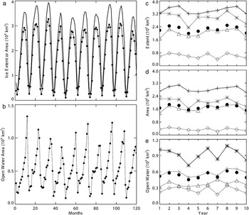
In terms of amplitudes, Fig. 19a shows integrated monthly sea ice extent (solid curve) and area (dotted curve) in 1 x 10⁶ km² for the Ross Sea sector for the decade for HiGEM1.1. Over this period, the model Ross Sea sea ice seems to be “spun up” in that the seasonal cycle repeats consistently over the decade, and there is no hint of an overall drift. In comparison with Zwally et al. (Reference Zwally, Comiso, Parkinson, Cavalieri and Gloersen2002) the peak extents and areas in HiGEM1.1 tend to be a little lower than observed. Figure 19b shows the resultant monthly open water area from the model. In comparison with observed, it is clear that the model captures the open water area seasonal pattern, with a distinct steep rise to a sharp peak followed by a rapid decline at the end of each year. However, the model has peaks regularly in excess of 1 x 10⁶ km² and minima < 0.2 x 10⁶ km² not seen in the observations.

Fig. 19

For 10 years of HiGEM1.1, monthly mean a. ice extent (plain curve) and area (dotted curve, 10⁶ km²), and b. open water (extent - area, 10⁶ km²) for Ross Sea sector starting in January (see text). HiGEM1.1 annual means for c. ice extent, d. ice area, and e. open water (extent - area, 10⁶ km²). In each part are plotted annual mean (•), and seasonal means per year for spring (*), summer (◊), autumn (▵), and winter (+) as defined by Zwally et al. (Reference Zwally, Comiso, Parkinson, Cavalieri and Gloersen2002).

The seasonal trends per year are shown in Fig. 19c–e, for HiGEM1.1 extent, area, and open water, respectively. The extent and area patterns match the observed in figs 6 & 12 in Zwally et al. (Reference Zwally, Comiso, Parkinson, Cavalieri and Gloersen2002), i.e. winter extents and areas exceed spring, then autumn, then summer extents and areas, with a distinct gap between the minima in summer and the rest of the seasons. For the open water, the model reproduces the observed change in distribution (fig. 18 in Zwally et al. Reference Zwally, Comiso, Parkinson, Cavalieri and Gloersen2002) in that spring open water areas now exceed winter values, and the minimum summer values are much closer to their respective autumn values. Again, the HadGEM1.1 patterns are similar to HiGEM1.1 (not shown).

Finally, Table II compares available long-term seasonal and annual values from Zwally et al. (Reference Zwally, Comiso, Parkinson, Cavalieri and Gloersen2002) with their respective estimates from HadGEM1.1 and HiGEM1.1. It is clear that, for extents and areas independent of either annual or seasonal, relative to the observations the HadGEM1.1 values are all larger, whereas those of HiGEM1.1 are all smaller. In terms of open water, HiGEM1.1 remains below observed (and this reflects the comparison for HiGEM1.1 in Fig. 19b), whereas the relatively coarser HadGEM1.1 returns a slight underestimate.

So, although the climate models suggest that the sea ice is in a relatively well spun up phase over the decade analysed, the long-term average amplitudes span the observed values from below (HiGEM1.1) and above (HadGEM1.1) for the Ross Sea sector. However, the seasonal patterns are consistent with the observations.

Discussion and conclusions

In this paper we have examined the circulation in the Ross Sea sector of the Southern Ocean in three complementary but different models (in terms of extent, forcing, physics and resolution). In general terms it is apparent that each model produces a broad gyral system spanning this sector, bounded largely to the north by the ACC, and by land to the south. As the resolution of the models increases, the eddy structures within the gyral system evolve, but basic large-scale patterns in the flow appear to have some bathymetric constraints. It is clear that the highest resolution of the operational model BRAN2.1 permits a much richer eddy structure within the gyre. Each model has its respective northern gyral extent overlying the ridge system in the Ross Sea sector consistent with observations. The east–west extent of the gyral system does not seem to have clear bathymetric constraints. Examination of the model flows suggest that the eastern boundary is around 136°W, in each model, with general recirculation within the gyre to the west, and clear eastward flow to the east with strong depth dependence in the flow direction. This location is consistent with deep flows reconstructed from float data by Davis (Reference Davis2005), and comparison with these flows suggests that BRAN2.1 might locate the eastern end of its gyre too far to the east. The westernmost end of the gyral system seems associated with a northwards diversion of the wider ACC flows. In HadGEM1.1 this occurs around 150°E, whereas in HiGEM1.1 this is shifted to the east and the western gyre is compressed in scale north–south relative to HadGEM1.1. BRAN2.1 shifts the western end of the western gyre further east again to around 155°E, and further compresses its northward extent.

Each model represents general east–west circulation across the Ross Sea shelf between the southern side of the gyres and the Antarctic continent. A total westward transport of some 8 Sv is found in each of the models for the Ross Sea sector. However, the way this is divided between the on- and off-shelf currents differs from model to model, suggesting sensitivity to model bathymetry and local forcing.

The comparison with depth-averaged flow on the Ross Sea continental shelf derived from longline reports suggests that the models are capturing important aspects of the flow even at these relatively coarse scales. In particular, along the shelf slope the models reproduce the flow direction and intensification toward Iselin Bank and at the Cape Adare end of the shelf. Examination of the density structure reveals that these flows are associated with slopes in the densest water (γⁿ > 28.27 kg m^-3), coincident with dips (‘V’s) in the upper isopycnal layers. These are found on the shelf, as well as over the shelf break where they are attributed to the Antarctic Slope Front and its associated current. Only the climate models in the intercomparison generate dense water on the Ross Sea shelf, and it is estimated that they transport some 4 Sv of this water northwards integrated along the 1000 m isobath of the Ross Sea continental slope. Furthermore, the resolution of HiGEM1.1 starts to represent deep layer patterns associated with troughs in the bathymetry on the shelf consistent with those in the Orsi & Wiederwohl (Reference Orsi and Wiederwohl2009) climatology.

Quasi-permanent eddies have been identified within the gyral system. One of them seems associated with deep bathymetric features (labelled as 2 in Fig. 3), eddy 3 seems bounded between the ACC and the Balleny Islands, while eddy 4 (associated with the formation of the far western reach of the gyral system) is the least distinct. These eddies become less distinct as the model resolution refines (from 1° for HadGEM1.1 down to 1/10° for BRAN2.1). This is especially true for the western part of the gyral system where the increasing flow complexity is certainly being dictated by the relatively detailed topography. Despite these differences, there is no doubt that the models are insistent on a wider gyral system spanning a significant portion of the Ross Sea sector.

Some of the gyral transports seem to be inversely related to the ACC transport in the models, i.e. as the ACC transport decreases the gyral transport increases, particularly so for the western gyre. This change is observed across different models so a strict model dependence cannot be immediately determined. Nevertheless, in a study using a single model by Schodlok et al. (Reference Schodlok, Wenzel, Schröter and Hellmer2008) in which changes in the ACC transport are induced by applying hydrographic constraints, a similar dependence is found between a decreasing ACC transport resulting in an increasing Weddell Gyre transport. These model results suggest that the hydrographic conditions underpinning the pathways of the ACC feedback into the representations of the Antarctic gyres. The gyre transports do seem correlated with ACC transport fluctuations, particularly in summer, and the ACC seasonal changes are intriguingly similar to that for the semi-annual oscillation. However, the models also reveal a wider degree of variability in gyral transport across the seasons, suggesting a number of time scales at play.

The best fit to the observed ACC transport is obtained by BRAN2.1 even though it has the poorest representation (in terms of sea ice and coastline) for the Ross Sea, but this is perhaps not surprising as it is an operational, data assimilating model. However, if we consider BRAN2.1 as producing the best dynamical estimate despite its physics limitations, then the peak transport of the main eastern gyre (measured across section 1 in Fig. 3) is around 33 Sv, relative to 30 Sv for HadGEM1.1 and 22 Sv for HiGEM1.1. This range of estimates appears typical (see the model solutions in Wang & Meredith Reference Wang and Meredith2008), so there remains some way to go before the wider Ross Sea circulation is more tightly constrained.

Overall it is clear that a number of processes at varying spatial and time scales contribute to the fluxes on and off the Ross Sea continental shelf. Even at 1/3°, HiGEM1.1 is perhaps only just starting to resolve the water mass distributions described by Orsi & Wiederwohl (Reference Orsi and Wiederwohl2009). However, the finer scales of the gravity currents associated with the outflowing bottom water (Gordon et al. Reference Gordon, Orsi, Muench, Huber, Zambianchi and Visbeck2009) are unresolved here, and Padman et al. (Reference Padman, Howard, Orsi and Muench2009) show that tides (not in the present models) can enhance deep water export from the shelf. Putting together consistent forcing fluxes for a regional Ross Sea model therefore remains a considerable challenge.

Is it a coincidence that the model with the finest scales (and hence most likely to capture more eddy activity) produces the best ACC transport? There is no doubt that eddy fluxes play an important role in the Southern Ocean, and the recent work by Screen et al. (Reference Screen, Gillett, Stevens, Marshall and Roscoe2009, and references therein) emphasises this fact by consideration of models of resolution 1°, 1/4°, and 1/12°, and showing that Southern Ocean sensitivity cannot be accurately represented without the eddies. But of course BRAN2.1 has a further advantage in that it assimilates data which may outweigh all other considerations.

What impact will ice shelves and their ocean cavities have on the wider gyral circulation? In model studies cooler and fresher shelf water is formed as a result of mixing open ocean water with sub-ice shelf freshwater. This increases shelf water stability (thereby reducing deep water formation rates), and sea ice thickens. The latter effect is evident in fig. 1 in Hellmer (Reference Hellmer2004), where ice flowing away from the Ross Ice Shelf is reduced in thickness by over 0.2 m. A modelling study by Stössel (Reference Stössel2008) suggests that reduced density water in the coastal region caused by the cavities can lead to increased westward coastal currents and enhancement of the associated cyclonic gyre. Furthermore, in a global ocean simulation, Losch (Reference Losch2008) finds deep water signatures of Ross Sea glacial meltwater as far north as 15°S. It is evident that ice shelves will introduce solution sensitivity on top of those explored in this paper, however, further model studies are needed to quantify their influence on the gyral circulation.

As a final consideration, Thorpe et al. (Reference Thorpe, Murphy and Watkins2007) show trajectories (potentially of krill) derived from ocean currents alone (in their case from a model), and then from a combination of ocean currents or sea ice motion. It is shown that quite different biological outcomes arise dependent on the biological strategy, regardless of uncertainties in the circulation. Thorpe et al. (Reference Thorpe, Murphy and Watkins2007) find that the large-scale krill distribution is likely dependent on the Antarctic Coastal Current and the sea ice motion, both impacting dispersal and retention in different regions around the Antarctic continent. Given the range of circulation estimates presented here, it is clear that large uncertainties remain in the modelling of the oceanography and its interaction with biology in the Southern Ocean.