1 Introduction
Characterizing the mean velocity profile (MVP) in the constant flux region of wall-bounded turbulent flows such as the atmospheric surface layer (ASL) has important implications for micro-meteorology, numerical weather prediction, air quality forecasting, hydrology, ecology and engineering. Unlike turbulent boundary layers studied in the laboratory that are not always thermally stratified, the ASL is constantly affected by both mean shear and thermal stratification arising from diabatic surface heating and cooling. The most successful theory describing the impact of thermal stratification on the MVP in the ASL is Monin–Obukhov similarity theory (MOST), where under the assumptions of quasi-stationarity, horizontal homogeneity, zero mean subsidence, and sufficiently high Reynolds number with coordinate system aligned with the mean wind direction, the normalized MVP is hypothesized to be a function of the stability parameter
 ${\it\zeta}$
alone:
 $$\begin{eqnarray}\displaystyle \frac{{\it\kappa}_{v}z}{u_{\ast }}\frac{\text{d}\overline{u}(z)}{\text{d}z}={\it\phi}_{m}({\it\zeta}), & & \displaystyle\end{eqnarray}$$
where the overbar denotes ensemble averaging and primes denote turbulent fluctuations from the mean. Here
 $u_{\ast }=(-\overline{u^{\prime }w^{\prime }})^{1/2}$
is the friction velocity,
 $\text{d}\overline{u}(z)/\text{d}z$
is the MVP,
 ${\it\kappa}_{v}=0.4$
is the von Kármán constant,
 ${\it\zeta}=z/L$
is the stability parameter that characterizes the relative importance of buoyancy production/destruction and shear production of turbulent kinetic energy (TKE),
 $z$
is the height above the ground surface (or above the zero-plane displacement for forest canopies),
 $L=-u_{\ast }^{3}/({\it\kappa}_{v}{\it\beta}\overline{w^{\prime }T^{\prime }})$
is the Obukhov length (Obukhov Reference Obukhov1946; Monin & Obukhov Reference Monin and Obukhov1954; Businger & Yaglom Reference Businger and Yaglom1971),
 ${\it\beta}=g/\overline{T}$
is the buoyancy parameter,
 $g$
is the gravitational acceleration and
 $T$
is the potential temperature. The ASL is classified as unstable when
 ${\it\zeta}<0$
and stable when
 ${\it\zeta}>0$
. Under neutral conditions (
 ${\it\zeta}=0$
),
 ${\it\phi}_{m}=1$
, and one can recover the logarithmic law of the wall. Since
 ${\it\phi}_{m}$
describes the departure of the MVP from the logarithmic profile due to thermal stratification, it is often called the ‘stability correction function’.
Because MOST is based on dimensional analysis (Obukhov Reference Obukhov1946; Monin & Obukhov Reference Monin and Obukhov1954), it cannot predict the functional form of
 ${\it\phi}_{m}$
, which needs to be determined empirically. Perhaps the most widely used empirical form of
 ${\it\phi}_{m}$
is the Businger–Dyer relation based on a fit to data from the Kansas experiment (Businger et al.
Reference Businger, Wyngaard, Izumi and Bradley1971; Dyer Reference Dyer1974; Businger Reference Businger1988), which under stable conditions is
 $$\begin{eqnarray}\displaystyle {\it\phi}_{m}({\it\zeta})=1+a_{m}{\it\zeta}, & & \displaystyle\end{eqnarray}$$
where
 $a_{m}$
was 4.7 when
 ${\it\kappa}=0.35$
was used (Businger et al.
Reference Businger, Wyngaard, Izumi and Bradley1971) and was 6.0 when
 ${\it\kappa}=0.4$
was used (Högström Reference Högström1988). Fits to various other datasets have suggested values of
 $a_{m}$
ranging from 4.7 to 9.4 (Högström Reference Högström1988). In our study, the Businger–Dyer relation refers to
 $a_{m}=6.0$
since
 ${\it\kappa}=0.4$
is used throughout our study and the variability of
 $a_{m}$
from other experiments is also considered. Note that most observational studies only report
 ${\it\phi}_{m}$
up to
 ${\it\zeta}=1{-}2$
due to data availability.
In spite of many other empirical relations and modifications to the Businger–Dyer relation, there has been a lack of theoretical arguments to explain the shape of these empirical curves and the connection to observed properties of turbulence (e.g. the integral length scales, spectra and the TKE budget). Recently, there has been renewed interest in understanding the MVP using phenomenological theories (Gioia et al.
Reference Gioia, Guttenberg, Goldenfeld and Chakraborty2010; Katul, Konings & Porporato Reference Katul, Konings and Porporato2011; Salesky, Katul & Chamecki Reference Salesky, Katul and Chamecki2013). Although these theories have been able to explain the MVP under neutral and unstable conditions, they have been found to be rather unsuccessful under stable conditions. Katul et al. (Reference Katul, Konings and Porporato2011) argued that the behaviour of
 ${\it\phi}_{m}$
under stable conditions is linked to the decrease in the size of momentum transporting turbulent eddies with increasing
 ${\it\zeta}$
, which could be characterized by the integral length scale of vertical velocity
 ${\it\Lambda}_{w}$
. However, in a subsequent study, Salesky et al. (Reference Salesky, Katul and Chamecki2013) found that including the integral length scales calculated from experimental data led to a significant under-prediction of
 ${\it\phi}_{m}$
by the phenomenological theory.
In the present article, we aim to address this shortcoming of the phenomenological theory (Gioia et al.
Reference Gioia, Guttenberg, Goldenfeld and Chakraborty2010; Katul et al.
Reference Katul, Konings and Porporato2011; Salesky et al.
Reference Salesky, Katul and Chamecki2013) and hypothesize that a more stringent estimate of the size of dominant momentum transporting eddies in the stable ASL under moderately stable (e.g.
 $0.2<{\it\zeta}<2$
) conditions is provided by the Ozmidov length scale
 $L_{OZ}=({\it\epsilon}/N^{3})^{1/2}$
where
 ${\it\epsilon}$
is the mean TKE dissipation rate and
 $N=({\it\beta}\text{d}\overline{T}(z)/\text{d}z)^{1/2}$
is the Brunt–Väisälä frequency (e.g. Dougherty Reference Dougherty1961; Ozmidov Reference Ozmidov1965; Smyth & Moum Reference Smyth and Moum2000; Bou-Zeid et al.
Reference Bou-Zeid, Higgins, Huwald, Meneveau and Parlange2010; Mater, Schaad & Venayagamoorthy Reference Mater, Schaad and Venayagamoorthy2013). This is because the Ozmidov length scale has the physical interpretation of the size of largest eddy unaffected by buoyancy (Mater et al.
Reference Mater, Schaad and Venayagamoorthy2013). This is also strongly motivated by recent studies that have proposed other similarity theories for stable ASLs (e.g. Zilitinkevich & Calanca Reference Zilitinkevich and Calanca2000; Sorbjan Reference Sorbjan2008, Reference Sorbjan2010), particularly one based on the Ozmidov scale (Grachev et al.
Reference Grachev, Andreas, Fairall, Guest and Persson2015). We stress that it is not our purpose to propose new functions for
 ${\it\phi}_{m}$
that better agree with observational data. Rather our goal is to explain the observed behaviour of
 ${\it\phi}_{m}$
(e.g. in the Businger–Dyer relation) from a phenomenological perspective and demonstrate the link between
 ${\it\phi}_{m}$
and observed properties of turbulence (such as the characteristic length and velocity scale of momentum transporting eddies), which further provides insights into the applicability of MOST under stable conditions.
2 Theory
In the constant flux region of turbulent boundary layers, the phenomenological model (Gioia et al.
Reference Gioia, Guttenberg, Goldenfeld and Chakraborty2010; Katul et al.
Reference Katul, Konings and Porporato2011) starts by assuming that the momentum flux transported by an isotropic eddy (i.e. having equivalent horizontal and vertical dimensions) of size
 $s$
that is located at
 $z$
can be expressed as
 $$\begin{eqnarray}\displaystyle u_{\ast }^{2}={\it\kappa}_{{\it\tau}}v(s)[\overline{u}(s+z)-\overline{u}(s-z)]\approx {\it\kappa}_{{\it\tau}}v(s)\frac{\text{d}\overline{u}(z)}{\text{d}z}2s, & & \displaystyle\end{eqnarray}$$
where
 ${\it\kappa}_{{\it\tau}}$
is a proportionality constant that can be later determined by imposing
 ${\it\phi}_{m}(0)=1$
. Here
 $v(s)$
is the eddy turnover velocity and
 $[\overline{u}(s+z)-\overline{u}(s-z)]$
denotes the mean velocity difference (i.e. net momentum per unit mass) across the eddy in the vertical direction. Invoking the attached eddy hypothesis (Townsend Reference Townsend1976), namely,
 $s=z$
, and using (1.1), the above equation can be simplified as
 $$\begin{eqnarray}\displaystyle 2\frac{{\it\kappa}_{{\it\tau}}}{{\it\kappa}_{v}}\frac{v(z)}{u_{\ast }}{\it\phi}_{m}=1. & & \displaystyle\end{eqnarray}$$
Estimates of
 $v(z)$
under neutral (Gioia et al.
Reference Gioia, Guttenberg, Goldenfeld and Chakraborty2010) and thermally stratified (Katul et al.
Reference Katul, Konings and Porporato2011; Salesky et al.
Reference Salesky, Katul and Chamecki2013) conditions have been discussed elsewhere and only the main results under thermally stratified conditions are presented here. Katul et al. (Reference Katul, Konings and Porporato2011) (hereafter K11) estimated
 $v(z)$
from the Kolmogorov ‘
 $4/5$
’ law for locally homogeneous and isotropic turbulence as
 $v(z)=(4/5{\it\epsilon}z)^{1/3}$
, where the mean TKE dissipation rate
 ${\it\epsilon}$
is obtained from the TKE budget equation (subjected to the same idealizations as MOST) as follows:
 $$\begin{eqnarray}\displaystyle {\it\epsilon}=\frac{u_{\ast }^{3}}{{\it\kappa}_{v}z}({\it\phi}_{m}-{\it\zeta}+{\it\gamma}_{1}), & & \displaystyle\end{eqnarray}$$
where
 ${\it\gamma}_{1}$
represents the imbalance between the total (shear + buoyant) production and dissipation of TKE, and has contributions from turbulent transport and pressure redistribution. It shall be demonstrated later from experimental data that the TKE imbalance is small (
 ${\it\gamma}_{1}\approx 0$
) under mild to moderate stratification. When (2.3) for
 ${\it\epsilon}$
is substituted into (2.2), it yields
 ${\it\gamma}_{0}({\it\phi}_{m}-{\it\zeta}+{\it\gamma}_{1})^{1/3}{\it\phi}_{m}=1$
, where
 ${\it\gamma}_{0}=(4/5)^{1/3}(2{\it\kappa}_{{\it\tau}}/{\it\kappa}_{v}^{4/3})$
is a constant. Upon imposing
 ${\it\phi}_{m}(0)=1$
under neutral conditions,
 ${\it\gamma}_{0}=1$
and, hence,
 $$\begin{eqnarray}\displaystyle ({\it\phi}_{m}-{\it\zeta}){\it\phi}_{m}^{3}=1, & & \displaystyle\end{eqnarray}$$
which is often called the O’KEYPS equation (named after Obukhov, Kazansky, Ellison, Yamamoto, Panofsky and Sellers) (Businger Reference Businger1988).
Until here the theory does not predict the MVP in agreement with experimental data, because the above derivations assume that the size of dominant eddies remains
 $z$
under all stability conditions. K11 recognized that the characteristic size of turbulent eddies can increase with unstable stratification and decrease with stable stratification. Denoting
 $s={\it\gamma}_{2}({\it\zeta})z$
(where
 ${\it\gamma}_{2}(0)=1$
) results in
 $$\begin{eqnarray}\displaystyle ({\it\phi}_{m}-{\it\zeta}){\it\phi}_{m}^{3}={\it\gamma}_{2}^{-4}. & & \displaystyle\end{eqnarray}$$
Note that this expression is slightly different from the formulation in K11 that only considered
 $s={\it\gamma}_{2}({\it\zeta})z$
in the expression of
 $v(s)$
but not in the expression of
 $[\overline{u}(s+z)-\overline{u}(s-z)]$
. A follow-up study by Salesky et al. (Reference Salesky, Katul and Chamecki2013) (hereafter S13) showed that changes in
 $s$
should be also accounted for in
 $[\overline{u}(s+z)-\overline{u}(s-z)]$
as stability changes. S13 further distinguished the vertical and horizontal characteristic length scales, which is not considered here due to the fact that S13 found from observational data that the anisotropy between the horizontal and vertical length scales becomes small under stable conditions.
2.1 Estimation of
 ${\it\gamma}_{2}$
in previous studies

K11 estimated
 ${\it\gamma}_{2}$
from the integral length scale of the vertical velocity (
 ${\it\Lambda}_{w}$
) using the Kansas experimental data under unstable conditions and interpolated the results to stable conditions. Although their resulting
 ${\it\phi}_{m}$
function matched the Businger–Dyer relation, it was later shown by S13 that this interpolated function does not agree with experimental data under stable conditions, especially when
 ${\it\zeta}>0.2$
(see figure 10 in S13). Thus, one can conclude that for stable conditions with
 ${\it\zeta}>0.2$
, neither
 $z$
nor
 ${\it\Lambda}_{w}$
is the appropriate length scale to capture the correct variation of
 ${\it\phi}_{m}$
.
2.2 Revised estimation of
${\it\gamma}_{2}$

Because the Ozmidov length scale is the smallest length scale affected by buoyancy in a stably stratified flow, it becomes a more stringent limit for the dominant eddy size in the stable ASL as vertical motions become increasingly suppressed by buoyancy (Dougherty Reference Dougherty1961; Ozmidov Reference Ozmidov1965; Smyth & Moum Reference Smyth and Moum2000; Bou-Zeid et al.
Reference Bou-Zeid, Higgins, Huwald, Meneveau and Parlange2010; Mater et al.
Reference Mater, Schaad and Venayagamoorthy2013). A plot of the Ozmidov scale (
 $L_{OZ}$
) normalized by
 $z$
as a function of the MOST stability parameter from two separate datasets (see Appendix), including one over a lake surface (Vercauteren et al.
Reference Vercauteren, Bou-Zeid, Parlange, Lemmin, Huwald, Selker and Meneveau2008; Li & Bou-Zeid Reference Li and Bou-Zeid2011) and the other over a grass surface (AHATS) (Salesky & Chamecki Reference Salesky and Chamecki2012; Salesky et al.
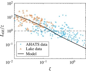
Reference Salesky, Katul and Chamecki2013), is displayed in figure 1, along with a theoretical prediction that will be derived in § 3. One can see that on average
 $L_{OZ}>z$
for
 ${\it\zeta}\lesssim 0.2$
but
 $L_{OZ}$
becomes smaller than
 $z$
for
 ${\it\zeta}\gtrsim 0.2$
where the original phenomenological theory fails (Salesky et al.
Reference Salesky, Katul and Chamecki2013), which motivates us to use
 $L_{OZ}$
as the characteristic size of momentum transporting eddies under such conditions. We note that there is large variability associated with
 $L_{OZ}$
estimated from observational data. This is due to the fact that
 $L_{OZ}$
is defined based on the mean dissipation rate of TKE and the Brunt–Väisälä frequency, both of which are difficult to compute from field measurements collected in the ASL, especially under stable conditions. The agreement between data and the theoretical prediction will be discussed in § 3.


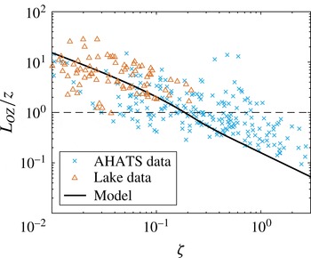
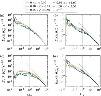
Figure 2 further shows how
 $L_{OZ}$
affects turbulent spectra from the AHATS dataset. The vertical grey line denotes the wavenumber
 $k_{1}=1/z$
and the point on the line denotes the Ozmidov wavenumber (i.e.
 $k_{1}=1/L_{OZ}$
). Figure 2(a–d) contain plots of the spectra of the streamwise (
 $E_{u}$
), transverse (
 $E_{v}$
), vertical (
 $E_{w}$
) velocity components and the TKE (
 $E_{tke}$
), respectively, averaged over five classes of
 ${\it\zeta}$
. One can see that the Ozmidov wavenumber (
 $1/L_{OZ}$
) increases as the stability increases, which is consistent with figure 1. The inertial subrange, whose scaling is the key in the original phenomenological theory and is assumed to be associated with the dominant momentum transporting eddy of size
 $1/z$
or
 $1/{\it\Lambda}_{w}$
(Katul et al.
Reference Katul, Konings and Porporato2011; Salesky et al.
Reference Salesky, Katul and Chamecki2013), is clearly more constrained by the Ozmidov wavenumber, especially in
 $E_{v}$
,
 $E_{w}$
and
 $E_{tke}$
. This supports the use of Ozmidov length scale in the phenomenological theory under stable conditions when
 $L_{OZ}<z$
.
Spectra of (a) streamwise velocity component
 $E_{u}$
, (b) transverse velocity component
 $E_{v}$
, (c) vertical velocity component
 $E_{w}$
and (d) TKE
 $E_{tke}$
calculated from AHATS data at
 $z=8.05$
m for several stability classes. The vertical line denotes the wavenumber where
 $k_{1}=1/z$
. The point plotted on the line for each stability class indicates the wavenumber associated with the median Ozmidov length scale for the stability class, i.e.
 $k_{1}=1/L_{OZ}$
. The number of blocks is 11, 16, 10, 18 and 12 for the five stability classes (as
 ${\it\zeta}$
increases).

This argument is further supported by a number of recent studies that have linked the MVP (and the mean temperature profile) to the spectra of vertical velocity (and the spectra of air temperature) based on solving the cospectral budgets of momentum flux (and sensible heat flux) (Banerjee & Katul Reference Banerjee and Katul2013; Katul et al.
Reference Katul, Li, Chamecki and Bou-Zeid2013, Reference Katul, Porporato, Shah and Bou-Zeid2014; Banerjee et al.
Reference Banerjee, Katul, Salesky and Chamecki2015, Reference Banerjee, Li, Juang and Katul2016; Li, Katul & Zilitinkevich Reference Li, Katul and Zilitinkevich2015b
). In these studies, the spectra of vertical velocity is idealized to be composed of a production range and an inertial subrange where the Kolmogorov ‘
 $-5/3$
’ scaling applies. The breakpoint between these two ranges is assumed to be characterized by
 $z$
or
 ${\it\Lambda}_{w}$
. However, it is clearly seen here that when
 ${\it\zeta}>0.2$
the Ozmidov scale becomes the appropriate length scale rather than
 $z$
or
 ${\it\Lambda}_{w}$
(Li, Katul & Bou-Zeid Reference Li, Katul and Bou-Zeid2015a
; Banerjee et al.
Reference Banerjee, Li, Juang and Katul2016).
Given that
 $L_{oz}$
is shown to be larger than
 $z$
(see figure 1) and the estimation of
 ${\it\gamma}_{2}$
in K11 agreed with data reasonably well when
 ${\it\zeta}\leqslant 0.2$
(see figure 10 in S13), we choose not to modify the estimation of
 ${\it\gamma}_{2}$
when
 ${\it\zeta}\leqslant 0.2$
. When
 ${\it\zeta}>0.2$
, however, the variation of
 ${\it\gamma}_{2}$
is modified to follow the variation of
 $L_{oz}$
with stability in our study. Upon imposing continuity of
 ${\it\gamma}_{2}^{-4}$
(i.e. the right-hand side of (2.5)) at
 ${\it\zeta}=0.2$
, the above argument gives
 ${\it\gamma}_{2}^{-4}=(L_{oz}/z)^{-4}+C$
where
 $C=-1+{\it\gamma}_{2}^{-4}({\it\zeta}=0.2)$
is a constant. Substituting it into (2.5) further yields for
 ${\it\zeta}>0.2$
,
 $$\begin{eqnarray}\displaystyle ({\it\phi}_{m}-{\it\zeta}){\it\phi}_{m}^{3}=(L_{oz}/z)^{-4}+C. & & \displaystyle\end{eqnarray}$$
3 Results
In order to obtain
 ${\it\phi}_{m}$
from (2.6),
 $L_{OZ}/z$
needs to be known a priori. Instead of fitting an empirical relation for
 $L_{OZ}/z$
, we derive a new expression for
 $L_{OZ}/z$
that is
 ${\it\phi}_{m}$
-dependent. Substituting
 ${\it\epsilon}$
calculated from (2.3) with
 ${\it\gamma}_{1}=0$
into
 $L_{oz}=({\it\epsilon}/N^{3})^{1/2}$
leads to
 $L_{oz}=(u_{\ast }^{3/2}({\it\phi}_{m}-{\it\zeta})^{1/2})/(({\it\kappa}_{v}z)^{1/2}({\it\beta}\text{d}\overline{T}/\text{d}z)^{3/4})$
. Given
 $u_{\ast }/({\it\kappa}_{v}z)=(\text{d}\overline{u}/\text{d}z){\it\phi}_{m}^{-1}$
,
 $$\begin{eqnarray}\displaystyle L_{oz}/z={\it\kappa}_{v}\frac{(\text{d}\overline{u}/\text{d}z)^{3/2}}{({\it\beta}\text{d}\overline{T}/\text{d}z)^{3/4}}{\it\phi}_{m}^{-3/2}({\it\phi}_{m}-{\it\zeta})^{1/2}. & & \displaystyle\end{eqnarray}$$
By definition, it can be shown that
 $({\it\beta}\text{d}\overline{T}/\text{d}z)/(\text{d}\overline{u}/\text{d}z)^{2}=Pr_{t}{\it\zeta}{\it\phi}_{m}^{-1}$
, where
 $Pr_{t}$
is the turbulent Prandtl number defined as
 $Pr_{t}=(-\overline{u^{^{\prime }}w^{^{\prime }}}/(\text{d}\overline{u}/\text{d}z))/(-\overline{w^{^{\prime }}T^{^{\prime }}}/(\text{d}\overline{T}/\text{d}z))$
, which when combined with (3.1) yields (Li et al.
Reference Li, Katul and Bou-Zeid2015a
; Banerjee et al.
Reference Banerjee, Li, Juang and Katul2016)
 $$\begin{eqnarray}\displaystyle L_{oz}/z={\it\kappa}_{v}(Pr_{t}{\it\zeta}{\it\phi}_{m})^{-3/4}({\it\phi}_{m}-{\it\zeta})^{1/2}. & & \displaystyle\end{eqnarray}$$
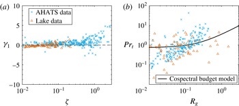
(a) The normalized imbalance between TKE production and dissipation calculated from observational data (
 ${\it\gamma}_{1}={\it\epsilon}{\it\kappa}_{v}z/u_{\ast }^{3}-({\it\phi}_{m}-{\it\zeta})$
). The dashed line indicates the value of zero. (b) The turbulent Prandtl number
 $Pr_{t}$
calculated from observational data and the cospectral budget model (the solid line). In this figure, the Businger–Dyer relation was used for
 ${\it\phi}_{m}$
.

Given a model for
 $Pr_{t}$
, equation (3.2) allows us to estimate the importance of
 $L_{oz}$
relative to
 $z$
. More importantly, the combination of (2.6) and (3.2) allows
 ${\it\phi}_{m}$
and
 $L_{OZ}/z$
to be solved numerically. The solid line in figure 1 shows
 $L_{oz}/z$
from solving (2.6) and (3.2). It is clear that the predicted Ozmidov length scale is larger than
 $z$
when
 ${\it\zeta}<0.2$
and is smaller than
 $z$
at higher stabilities. Despite a fairly large amount of scatter in the data and some biases at
 ${\it\zeta}>1$
, one can see that the theoretical curve captures the average behaviour of
 $L_{OZ}/z$
under mildly to moderately stable conditions (
 ${\it\zeta}<1-2$
).
Before we examine the resulting
 ${\it\phi}_{m}$
from solving (2.6) and (3.2), the assumptions leading to (3.2) are analyzed. The first assumption is that the TKE imbalance
 ${\it\gamma}_{1}\approx 0$
, which is also used in K11 and S13. Figure 3(a) shows the computed
 ${\it\gamma}_{1}$
using data from two field experiments. It is clear from figure 3(a) that
 ${\it\gamma}_{1}$
is close to zero under mildly to moderately stable conditions. At high stabilities, there are large uncertainties associated with
 ${\it\gamma}_{1}$
and the AHATS data suggest positive values of
 ${\it\gamma}_{1}$
when
 ${\it\zeta}>1$
. The other assumption is the cospectral budget model for
 $Pr_{t}$
, which has been extensively validated under both stable and unstable conditions using field experimental data, laboratory data, large-eddy simulation and direct numerical simulation results (Katul et al.
Reference Katul, Li, Chamecki and Bou-Zeid2013, Reference Katul, Porporato, Shah and Bou-Zeid2014; Li et al.
Reference Li, Katul and Zilitinkevich2015b
). Here additional data are used to validate the model. It can be seen that large scatter prevents a conclusive statement from being generalized from figure 3(b) but the data seem to show an increasing trend that is consistent with the cospectral budget model. Revisiting the validation done in previous studies (Katul et al.
Reference Katul, Li, Chamecki and Bou-Zeid2013, Reference Katul, Porporato, Shah and Bou-Zeid2014; Li et al.
Reference Li, Katul and Zilitinkevich2015b
) also suggests that field experimental data generally show larger scatter as compared with laboratory data and numerical simulations. Note the gradient Richardson number (
 $R_{g}=({\it\beta}\text{d}\overline{T}/\text{d}z)/(\text{d}\overline{u}/\text{d}z)^{2}$
) is used here to indicate atmospheric stability due to the ‘self-correlation’ between
 $Pr_{t}$
and
 ${\it\zeta}$
when observational data are used to calculate both (Esau & Grachev Reference Esau and Grachev2007; Grachev et al.
Reference Grachev, Andreas, Fairall, Guest and Persson2007).
The results presented so far have demonstrated that the two assumptions made in arriving at (3.2) are generally satisfied in ‘idealized’ stably stratified ASLs under mildly to moderately stable conditions. However, the first assumption (i.e.
 ${\it\gamma}_{1}=0$
) is invalid under higher stabilities and there are large uncertainties associated with turbulent statistics such as
 $Pr_{t}$
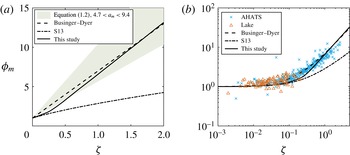
. Now (3.2) and (2.6) are combined to solve for
 ${\it\phi}_{m}$
numerically, which is then compared with the widely used Businger–Dyer relation (along with data from field experiments), as shown in figure 4. Also shown is the result from S13 where
 ${\it\gamma}_{2}$
was based on
 ${\it\Lambda}_{w}$
(i.e.
 ${\it\gamma}_{2}$
is set to
 $f({\it\zeta})$
in S13). As one can see,
 ${\it\phi}_{m}$
calculated from the present theoretical framework improves over S13 when
 ${\it\zeta}>0.2$
and is in better agreement with the observational data (at least in the stable regime examined here). The root-mean-square errors between observations and modeled
 ${\it\phi}_{m}$
values using the Businger–Dyer relation, the relation from this study, and the relation from the study of S13 are 1.1, 1.1 and 1.8, respectively, suggesting that the original phenomenological theory is significantly improved by incorporating the Ozmidov scale.
(a) The stability correction function
 ${\it\phi}_{m}$
from this study, the study of S13 and the empirical Businger–Dyer relation. (b) Similar to (a) except in the log–log scale and with the lake and AHATS data.

4 Discussion and conclusions
This study has aimed to link the behaviour of
 ${\it\phi}_{m}$
(as observed from data and empirical fits to data such as the Businger–Dyer relation) to the change in the size of momentum transporting eddies under stable conditions. Previous studies showed that a phenomenological theory for thermally stratified ASLs explained the MVP under unstable conditions, but struggled to capture its behaviour under stable conditions, especially when
 ${\it\zeta}>0.2$
(Katul et al.
Reference Katul, Konings and Porporato2011; Salesky et al.
Reference Salesky, Katul and Chamecki2013). We hypothesize here that this is due to the change in the characteristic size of turbulent eddies. We find that the Ozmidov length scale
 $L_{OZ}$
becomes smaller than the distance from the wall
 $z$
for
 ${\it\zeta}>0.2$
and becomes a more stringent limitation for the size of momentum transporting eddies.
An expression for the Ozmidov length scale is derived in our study based on two assumptions: (1) the TKE budget equation is in equilibrium and (2) a cospectral budget model can be used for describing the turbulent Prandtl number
 $Pr_{t}$
. These assumptions have been validated here using two datasets collected in the stable ASL. Under mildly to moderately stable conditions (e.g.
 ${\it\zeta}<1-2$
), the two assumptions are broadly supported by these new field experimental data.
When the variation of Ozmidov length scale with stability over
 ${\it\zeta}>0.2$
is used in the phenomenological theory to approximate how the size of dominant turbulent eddies changes with stability, the resulting
 ${\it\phi}_{m}$
is in good agreement with the Businger–Dyer relation and experimental data. As a result, the modification explains the failure of the original phenomenological theory and provides a theoretical justification for formulating similarity theories based on the Ozmidov length scale under moderately stable conditions (e.g. Grachev et al.
Reference Grachev, Andreas, Fairall, Guest and Persson2015).
It should be emphasized that the phenomenological theory may not be applicable under strongly stable conditions (e.g.
 ${\it\zeta}>1-2$
). This is because of potential failure of several key assumptions (e.g. the balance between TKE production and dissipation) as already alluded to in figure 3 and the fact that the phenomenological theory depends on the Kolmogorov scaling. Recent field experiments have shown that the inertial subrange vanishes and the scaling deviates from the Kolmogorov theory when the atmospheric stability exceeds some threshold (Grachev et al.
Reference Grachev, Andreas, Fairall, Guest and Persson2013; Li et al.
Reference Li, Katul and Bou-Zeid2015a
). Although turbulence might still exist, it no longer follows the traditional Kolmogorov scaling or even does not have a distinct inertial subrange. The behaviour of MVP under strongly stable conditions and its connection with high-order turbulent statistics such as the spectra remains an open question (Mahrt Reference Mahrt2014).
Acknowledgements
The lake data were collected by the Environmental Fluid Mechanics and Hydrology Laboratory of Professor M. Parlange at L’Ècole Polytechnique Fédérale de Lausanne. We thank Professor Parlange for sharing the data with us. The AHATS data were collected by NCAR’s Integrated Surface Flux Facility.
Appendix. Data
The lake dataset includes measurements of three-dimensional velocity and temperature at 20 Hz frequency and at four different heights. Details about the dataset, quality control measures and calculations of 30 min turbulent fluxes can be found elsewhere (Vercauteren et al.
Reference Vercauteren, Bou-Zeid, Parlange, Lemmin, Huwald, Selker and Meneveau2008; Li & Bou-Zeid Reference Li and Bou-Zeid2011; Li, Bou-Zeid & de Bruin Reference Li, Bou-Zeid and de Bruin2012; Li et al.
Reference Li, Katul and Bou-Zeid2015a
). The mean velocity and temperature gradients, which are needed in the calculations of
 $Pr_{t}$
and
 $L_{OZ}$
, are obtained by fitting second-order polynomial functions to the mean velocity and temperature at four levels and then taking the derivatives of the fitted functions (Högström Reference Högström1988). In addition, two methods were used to calculate the mean dissipation rate of TKE as presented elsewhere (Li, Katul & Gentine Reference Li, Katul and Gentine2016). The first method calculated
 ${\it\epsilon}$
from the second-order longitudinal velocity structure function following
 ${\it\epsilon}=(0.3535)[D_{uu}(r)^{3/2}/r]$
and the second method calculated
 ${\it\epsilon}$
from the third-order longitudinal structure function
 $D_{uuu}(r)$
following
 ${\it\epsilon}=-(5/4)[D_{uuu}(r)]/r$
(Stull Reference Stull1988), where
 $D_{uu}(r)=\overline{[u(x+r)-u(x)]^{2}}$
,
 $D_{uuu}(r)=\overline{[u(x+r)-u(x)]^{3}}$
and
 $r$
is the separation distance aligned along the mean wind direction and is set to
 $z/2$
following previous work (Li et al.
Reference Li, Bou-Zeid and de Bruin2012). The two methods yield similar estimates of
 ${\it\epsilon}$
consistent with other studies (Bou-Zeid et al.
Reference Bou-Zeid, Higgins, Huwald, Meneveau and Parlange2010).
The AHATS dataset was collected over level and horizontally homogeneous terrain covered by short grass stubble. In the present study we used data from the profile tower, with 60 Hz measurements of three-dimensional velocity and temperature at six heights. Details of the dataset and the selection and analysis procedure are described elsewhere (Salesky & Chamecki Reference Salesky and Chamecki2012; Salesky et al.
Reference Salesky, Katul and Chamecki2013). Fluxes were calculated from 20 Hz data using 27.3 min blocks. Spectra were calculated from the 60 Hz data using 36.4 min blocks (
 $2^{17}$
points) and averaged in logarithmically spaced bins of wavenumber to reduce the noise at high wavenumbers.