1 Introduction
Flows over superhydrophobic surfaces have received considerable attention in recent years due to their potential for viscous drag reduction. The reduction of solid–liquid contact area for a liquid in the Cassie state and the low-shear stress on the liquid–gas interfaces (menisci) result in a lubricating effect. This effect has been quantified via an (apparent hydrodynamic) slip length, which has been determined by experiments, numerical solutions and analytical techniques for surfaces textured with pillars, holes and ridges (Philip Reference Philip1972a,Reference Philipb; Vinogradova Reference Vinogradova1995; Lauga & Stone Reference Lauga and Stone2003; Cottin-Bizonne et al. Reference Cottin-Bizonne, Barentin, Charlaix, Bocquet and Barrat2004; Ou, Perot & Rothstein Reference Ou, Perot and Rothstein2004; Ou & Rothstein Reference Ou and Rothstein2005; Davies et al. Reference Davies, Maynes, Webb and Woolford2006; Maynes, Webb & Davies Reference Maynes, Webb and Davies2008; Belyaev & Vinogradova Reference Belyaev and Vinogradova2010).
The case of parallel ridges in particular, where an array of ridges is oriented parallel to the flow direction, has received much attention owing to their advantage in drag reduction compared to transverse ridges (oriented perpendicular to the flow direction) (Teo & Khoo Reference Teo and Khoo2009) and also recently their promise in convective heat transfer compared to pillars (Enright et al. Reference Enright, Hodes, Salamon and Muzychka2014; Lam, Hodes & Enright Reference Lam, Hodes and Enright2015). Most theoretical and computational studies assumed that the menisci that span the tips of the ridges are flat for simplicity until Steinberger et al. (Reference Steinberger, Cottin-Bizonne, Kleimann and Charlaix2007) demonstrated experimentally the significant impact of curvature for a mattress of protruding bubbles, where they showed the lubrication effect can be entirely negated for transverse ridges if the menisci protrude far enough into the flow. This was then corroborated qualitatively by Hyväluoma & Harting (Reference Hyväluoma and Harting2008) using two-phase lattice Boltzmann simulations. Experiments by Tsai et al. (Reference Tsai, Peters, Pirat, Wessling, Lammertink and Lohse2009) concluded that meniscus curvature could explain the overestimate of slip in previous flat-interface theoretical models. Consequently, analytical models of shear flows accounting for weak protrusion (Sbragaglia & Prosperetti Reference Sbragaglia and Prosperetti2007; Crowdy Reference Crowdy2017), and arbitrarily large protrusion were developed (Davis & Lauga Reference Davis and Lauga2009; Crowdy Reference Crowdy2010, Reference Crowdy2016; Schnitzer Reference Schnitzer2016, Reference Schnitzer2017), for both transverse and longitudinal ridges. Computational studies with meniscus protrusion include Teo & Khoo (Reference Teo and Khoo2010) for pressure-driven flows and Ng & Wang (Reference Ng and Wang2011) for shear flows. A comprehensive study by Game et al. (Reference Game, Hodes, Keaveny and Papageorgiou2017) used a Chebyshev collocation scheme to account not only for arbitrary meniscus protrusion on longitudinal ridges, but also subphase gas viscosity, cavity depth and channel-edge effects due to a finite spanwise geometry. A similar study using finite volume and eigenfunction expansion methods was undertaken by Li, Alame & Mahesh (Reference Li, Alame and Mahesh2017). Other recent studies have employed boundary element methods to investigate meniscus protrusion for arbitrary ridge orientation (Ageev, Golubkina & Osiptsov Reference Ageev, Golubkina and Osiptsov2018) or to account for interface deformation (for lubricant-filled cavities) (Alinovi & Bottaro Reference Alinovi and Bottaro2018).
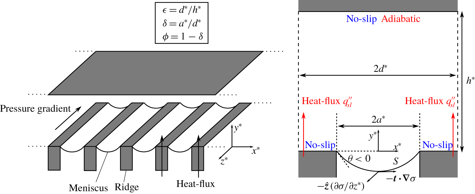
Many asymptotic techniques exploiting the multi-scale nature of superhydrophobic ridged surfaces have been essential to the development of analytical results for slip length, but also insight into the importance of different physical factors affecting it. Sbragaglia & Prosperetti (Reference Sbragaglia and Prosperetti2007) accounted for weak protrusion (small meniscus curvature) in a channel with longitudinal ridges on one wall by performing boundary perturbation, reducing the problem to a pair of dual-series equations. Wang, Teo & Khoo (Reference Wang, Teo and Khoo2014) repeated the analysis for a pipe geometry, and Kirk, Hodes & Papageorgiou (Reference Kirk, Hodes and Papageorgiou2017) extended it to the convective heat transfer problem in a channel with ridges on both walls. Such small curvature expansions were shown to have a good range of validity compared to numerical solutions, with the slip length formulae accurate to within 10 % error for protrusion angles  $\unicode[STIX]{x1D703}$ (see figure 1 for the channel geometry and definition of
 $\unicode[STIX]{x1D703}$) in the range -40° ≲𝜃≲ 40° (Teo & Khoo Reference Teo and Khoo2010), and the Nusselt number formulae this accurate for the even larger range -87° ≲𝜃≲ 50° (Game et al. Reference Game, Hodes, Kirk and Papageorgiou2018). These accuracy bounds are valid for ridge periods as large as the channel height, and for any slip fraction, which corresponds to the ratio of cavity width to ridge period. To produce slip length formulae valid for any protrusion angle up to ±90°, Crowdy (Reference Crowdy2010, Reference Crowdy2016) used conformal mapping techniques in the ‘dilute’ meniscus packing limit (small slip fraction), whereas Schnitzer (Reference Schnitzer2017) considered (for
 $0\leqslant \unicode[STIX]{x1D703}\leqslant 90^{\circ }$) the ‘dense’ packing limit (slip fraction close to one), both for shear flows. The connection between these shear flows and pressure-driven channel flows was explained by Kirk (Reference Kirk2018) who considered the small-ridge-period limit, with exponentially small error, using a matched asymptotic expansion. Despite several nested asymptotic limits, the resulting slip formulae in the dilute limit compared to finite-element solutions were shown to be remarkably accurate over an extended range of validity, i.e. for ridge periods not small but large enough for the menisci to contact the opposing (flat) channel surface. The dense packing limit was not considered in Kirk (Reference Kirk2018), but Yariv & Schnitzer (Reference Yariv and Schnitzer2018) considered this limit, albeit only for semi-circular bubbles, with ridges on both channel walls, where a plug flow occurs to leading order.
Most of the aforementioned research considers adiabatic flows. Studies on diabatic ones, i.e. those in the presence of heat transfer, are discussed by Game et al. (Reference Game, Hodes, Kirk and Papageorgiou2018). An application of them is enhanced microchannel cooling of microelectronics, either in a direct liquid cooling configuration, where liquid flows through a heat-dissipating semiconductor, or an indirect one, where it flows through a cold plate. The pioneering study on direct liquid cooling in conventional (smooth) microchannels was by Tuckerman & Pease (Reference Tuckerman and Pease1981). Water was pumped through a bank of 50 μm-wide  $\times$ 302 μm-tall × 1 cm long microchannels etched into a 1 cm × 1 cm footprint × 400 μm-thick Si test specimen. In the key experiment, the pressure drop across the microchannels was 214 kPa and a uniform heat flux of 790 W cm-2 was imposed, resulting in a modest 71 °C temperature rise on account of the high convection heat transfer coefficient; 31 % of the thermal resistance was caloric, i.e. on account of the bulk temperature rise of the water with the rest being primarily on account of the surface-to-bulk liquid temperature difference.
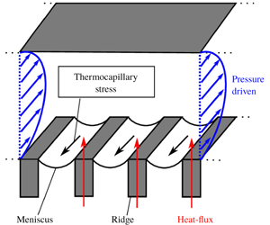
Schematic of the pressure-driven channel flow aligned with a periodic array of ridges of period  $2d^{\ast }$ and spacing
 $2a^{\ast }$. Circular cross-section menisci contact the ridge corner at angle
 $\unicode[STIX]{x1D703}$ (with
 $\unicode[STIX]{x1D703}<0$ corresponding to downward protrusion). The top wall is flat and a distance
 $h^{\ast }$ from the ridge tips. On the meniscus, only thermocapillary stresses are shown for clarity.

Recently, Galinstan, a (non-toxic) liquid metal, has emerged as a promising alternative to water for microchannel cooling because of its favourable thermophysical properties (Hodes et al. Reference Hodes, Zhang, Lam, Wilcoxon and Lower2014; Lam et al. Reference Lam, Hodes and Enright2015; Zhang et al. Reference Zhang, Hodes, Lower and Wilcoxon2015). It is a eutectic alloy of gallium, indium and tin that melts at -19 °C, boils above 1300 °C, has a density of 6440 kg m-3 and a viscosity of 0.0024 kg m-1 s-1 at 20 °C, i.e. approximately 2.5 times that of water (Geratherm 2009; Hodes et al. Reference Hodes, Zhang, Lam, Wilcoxon and Lower2014). Its volumetric heat capacity ( $\unicode[STIX]{x1D70C}c_{p}$) is less than half of that of water (Hodes et al. Reference Hodes, Zhang, Lam, Wilcoxon and Lower2014). A key advantage of Galinstan relative to water is that its thermal conductivity (16.5 W m-1 K-1) is 28 times larger (Geratherm 2009) and it remains in the liquid phase. An experiment by Zhang et al. (Reference Zhang, Hodes, Lower and Wilcoxon2015) resulted in a lower thermal resistance than measured by Tuckerman and Pease (0.077 °C/W versus 0.090 °C/W) at a higher heat flux (i.e. 1214 W cm-2). Caloric resistance dominates convective resistance in the case of Galinstan-based microchannel cooling on account of its high viscosity and low volumetric heat capacity. Consequently, lubrication, as may be achieved using superhydrophobic microchannels, is of great benefit. Indeed, Lam et al. using apparent slip lengths and Nusselt numbers in the literature (Maynes & Crockett Reference Maynes and Crockett2014; Kirk et al. Reference Kirk, Hodes and Papageorgiou2017) showed in a modelling study that a net enhancement can be achieved by texturing the microchannels with parallel ridges, despite the loss of surface area for solid-to-liquid heat transfer on account of menisci. (This was not possible with water, where the loss of heat transfer surface area was intolerable.) However, secondary effects such as phase change, thermocapillary stress and curvature along menisci were not captured in the study. The present analysis enables one to capture the latter two effects’ impact on flow (caloric) resistance. Also relevant is that the surface tension of Galinstan is approximately 7.4 times that of water and the advancing contact angle of Galinstan on Teflon is 161. 2° (cf. 110° for water) (Liu, Sen & Kim Reference Liu, Sen and Kim2012). Consequently, approximately 20 times the pressure difference may be imposed across a microchannel while maintaining the Cassie state when the liquid is Galinstan rather than water.
In microchannel cooling, the temperature of the liquid changes along the menisci, in both the streamwise and transverse directions, producing shear stresses (Marangoni stresses) due to variations in surface tension that impact the flow resistance. Marangoni stresses can be a significant detriment to lubrication, as recent experimental work on surfactants has shown (Peaudecerf et al. Reference Peaudecerf, Landel, Goldstein and Luzzatto-Fegiz2017; Song et al. Reference Song, Song, Hu, Du, Du, Choi and Rothstein2018). In particular, surfactant gradients on a meniscus of finite extent in the flow direction can produce adverse stresses large enough to completely immobilise the meniscus, even for trace amounts of surfactants – a possible explanation for the lubrication in experiments being much lower than predicted for parallel or transverse ridges. Another plausible explanation recently presented is the often-neglected slow streamwise variation of meniscus curvature as the liquid pressure decreases in the flow direction (Game, Hodes & Papageorgiou Reference Game, Hodes and Papageorgiou2019).
The effect of thermocapillary stress on heated superhydrophobic surfaces was first considered for droplets, with convection within the drops arising from vertical temperature gradients (Tam et al. Reference Tam, von Arnim, McKinley and Hosoi2009). The effect of thermocapillary stresses on slip length was first studied by Baier, Steffes & Hardt (Reference Baier, Steffes and Hardt2010), who considered flow driven by thermocapillary stress, with no background pressure gradient present. A constant streamwise temperature gradient was imposed along the ridges and the slip length for a semi-infinite domain was computed utilising the Lorentz reciprocal theorem. The slip lengths were consistent with their numerical simulations, and it was found that imposing temperature gradients of the order of 10 °C per cm may pump water through microchannels at mean velocities of the order of several mm per second. This type of thermocapillary-driven flow proposed by Baier et al. has been further extended to internal flows for temperature gradients imposed either longitudinally or transverse to the ridges (Yariv Reference Yariv2018; Yariv & Crowdy Reference Yariv and Crowdy2019). For longitudinally imposed temperature gradients, Yariv (Reference Yariv2018) developed a simple transformation to convert solutions from the literature for internal pressure-driven flows to those for thermocapillary-stress-driven internal (creeping) flows when the menisci are flat. He also used matched asymptotic expansions to resolve the transverse flow and temperature fields in the small ridge-period-to-channel-height limit. The analysis was extended to temperature gradients imposed transverse to the ridges in Yariv & Crowdy (Reference Yariv and Crowdy2019) in several geometric limits (small solid fraction limit, and large- or small-ridge-period-to-channel height limits). Very recently Yariv & Crowdy (Reference Yariv and Crowdy2020) extended the original longitudinal flow for  $\unicode[STIX]{x1D703}=0^{\circ }$ in Baier et al. (Reference Baier, Steffes and Hardt2010) to the special case of
 $\unicode[STIX]{x1D703}=+90^{\circ }$ in the densely packed limit, and is the only such study to consider non-flat menisci.
Hodes et al. (Reference Hodes, Kirk, Karamanis and MacLachlan2017) considered the effect of thermocapillary stress on a pressure-driven background flow parallel to ridges on one wall of a channel, which were held at constant heat flux. They accounted for thermocapillary stress in both the streamwise and transverse directions, the latter inducing a transverse cell flow. The menisci were assumed to be flat, allowing an exact solution to be found for the decoupled streamwise flow. Thermocapillary stress was found to have a significant impact on slip, with slip degradation (and in some cases negative slip lengths for water) for positive heat flux. For significant inertia in the transverse direction, full numerical solutions capturing the transverse flow field were also performed.
As all previous studies on thermocapillary stress have assumed a flat meniscus (except Yariv & Crowdy (Reference Yariv and Crowdy2020) for thermocapillary-driven flow), in this paper we study the coupled effects of thermocapillary stress and meniscus curvature on pressure-driven flow. Whereas Baier et al. (Reference Baier, Steffes and Hardt2010), Yariv (Reference Yariv2018) and Yariv & Crowdy (Reference Yariv and Crowdy2019, Reference Yariv and Crowdy2020) impose a linear temperature gradient via the solid substrate to generate a flow in that direction, here (and in Hodes et al. Reference Hodes, Kirk, Karamanis and MacLachlan2017) the only condition imposed on the temperature field is a constant heat flux along the length of the ridges. A linear temperature gradient in the streamwise direction then arises naturally from advection due to the pressure gradient, and the fully developed assumption. In order to account for thermocapillary stresses on a meniscus of fixed shape, i.e. a circular arc, we identify a transverse capillary number  $Ca_{\bot }$ that must be small. Further, when the transverse Reynolds number
 $Re_{\bot }$ is small, the streamwise problem can be completely decoupled from the transverse cell flow, reducing to the (nonlinear) problem (3.10)–(3.14) for the streamwise velocity. The thermocapillary stress is constant, but its magnitude depends on the unknown flow rate, since the temperature gradient is induced by the flow itself (along with a constant heat flux), not externally imposed.
To solve for the streamwise velocity, we employ the accurate asymptotic methods developed for curved menisci, and modify them appropriately to account for the additional interfacial stresses. The main approach relies on a matched asymptotic expansion in the small-ridge-period (or ‘aspect ratio’) limit, as in Kirk (Reference Kirk2018), and we take two different further limits: (i) small meniscus curvature (close to flat) using boundary perturbation; and (ii) arbitrarily curved menisci that are dilutely packed (i.e. small slip fraction). These limits are complementary and, to the orders presented here, are good approximations (with an error of only a few per cent) up to  $|\unicode[STIX]{x1D703}|\lesssim 40^{\circ }$ and slip fractions
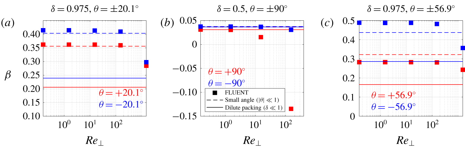
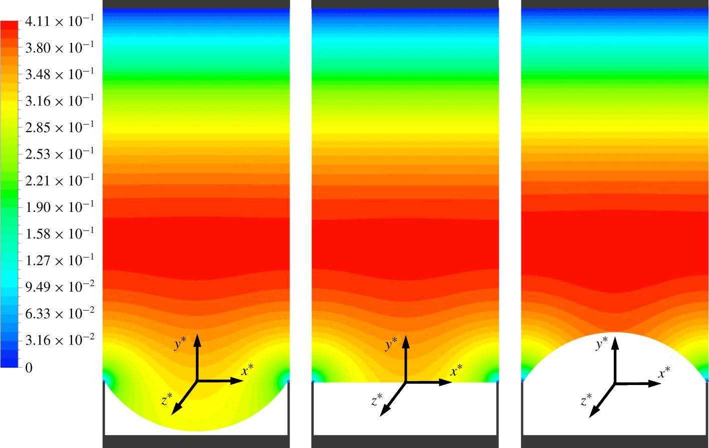
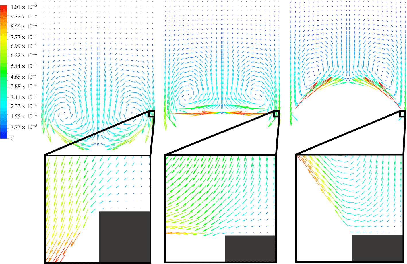
 $\unicode[STIX]{x1D6FF}\lesssim 0.75$, respectively, when compared against full numerical solutions. In the analysis we focus on the effect of heat transfer on the hydrodynamic problem only, and do not give results for the temperature problem or Nusselt number. However, when inertia in the transverse flow is not negligible, we solve for the full coupled hydrodynamic and thermal problems numerically and demonstrate that inertia is always detrimental to slip, for negative and positive protrusion angles.
The structure of the paper is as follows. The full three-dimensional problem for the coupled flow and temperature fields is formulated in § 2. The scaling and decoupling of the streamwise flow is in § 3, with the various asymptotic solutions presented in § 4. The results from these solutions are given in § 5, and compared with numerical solutions of the full coupled problem in § 6, with the conclusions in § 7.
2 Formulation
We consider steady, hydrodynamically and thermally fully developed flow in a parallel plate channel, the bottom wall patterned with uniformly spaced parallel ridges aligned with the flow direction, as in figure 1. The top wall could be a flat no-slip surface (Sbragaglia & Prosperetti Reference Sbragaglia and Prosperetti2007; Teo & Khoo Reference Teo and Khoo2009, Reference Teo and Khoo2010), or patterned identically to the lower wall so that the flow is symmetric about the centre plane of the channel (Kirk et al. Reference Kirk, Hodes and Papageorgiou2017). We will focus on the former case, although selected results for the latter case are included in appendix C. Surface tension maintains the liquid in the Cassie state, i.e. the liquid contacts the ridges only at their tips, and the cavities between ridges are filled with trapped gas. The pressure difference at the liquid–gas interfaces (menisci) results in protrusion into or out of the cavities, forming circular arcs  $S$ of angle
 $\unicode[STIX]{x1D703}$ with the horizontal at the ridge corners. The ridge structuring and resulting flow is periodic with period
 $2d^{\ast }$ and the width of each cavity (or distance between adjacent ridges) is
 $2a^{\ast }$. One period window,
 $x^{\ast }\in [-d^{\ast },d^{\ast }]$, with the cavity located at
 $x^{\ast }\in [-a^{\ast },a^{\ast }]$, is shown in figure 1. We note that an asterisk will denote that a quantity is dimensional. The channel spacing, i.e. the distance from the tips of the ridges to the top surface, is denoted
 $h^{\ast }$. The geometry of the channel can be characterised by two length ratios: the ratio of (half) the period to channel spacing,
 $\unicode[STIX]{x1D716}=d^{\ast }/h^{\ast }$; and the ratio of cavity width to period,
 $\unicode[STIX]{x1D6FF}=a^{\ast }/d^{\ast }$ (the cavity or slip fraction). The flow is driven by a constant pressure gradient
 $\unicode[STIX]{x2202}p^{\ast }/\unicode[STIX]{x2202}z^{\ast }$ in the
 $z^{\ast }$ direction.
Heat is supplied to (or removed from) the liquid where it contacts the ridges, i.e. their tips, where a constant heat flux boundary condition is imposed. If we assume that the direction of heat flow is into the domain, i.e. the heat flux  $q_{sl}^{\prime \prime }$ through the ridge tips per unit area is positive, then the temperature of the liquid will increase in the streamwise direction
 $z^{\ast }$, but decrease towards the centre of the meniscus in the transverse direction. Thus, as we will include the variation of surface tension at the meniscus with respect to temperature, thermocapillary stresses are induced at the meniscus in both directions. (However, we will assume that this variation is small enough that the meniscus shape is still approximately a circular arc, as in the adiabatic case – see § 3 for detailed scaling arguments.) The transverse stresses induce a velocity field in the cross-plane; therefore, the velocity is three-dimensional, i.e.
 $\boldsymbol{u}^{\ast }=(u^{\ast },v^{\ast },w^{\ast })$, and satisfies the Navier–Stokes and continuity equations,
 $$\begin{eqnarray}\displaystyle & \displaystyle \unicode[STIX]{x1D70C}\left(u^{\ast }\frac{\unicode[STIX]{x2202}u^{\ast }}{\unicode[STIX]{x2202}x^{\ast }}+v^{\ast }\frac{\unicode[STIX]{x2202}u^{\ast }}{\unicode[STIX]{x2202}y^{\ast }}\right)=-\frac{\unicode[STIX]{x2202}p^{\ast }}{\unicode[STIX]{x2202}x^{\ast }}+\unicode[STIX]{x1D707}\left(\frac{\unicode[STIX]{x2202}^{2}u^{\ast }}{\unicode[STIX]{x2202}x^{\ast 2}}+\frac{\unicode[STIX]{x2202}^{2}u^{\ast }}{\unicode[STIX]{x2202}y^{\ast 2}}\right), & \displaystyle\end{eqnarray}$$
 $$\begin{eqnarray}\displaystyle & \displaystyle \unicode[STIX]{x1D70C}\left(u^{\ast }\frac{\unicode[STIX]{x2202}v^{\ast }}{\unicode[STIX]{x2202}x^{\ast }}+v^{\ast }\frac{\unicode[STIX]{x2202}v^{\ast }}{\unicode[STIX]{x2202}y^{\ast }}\right)=-\frac{\unicode[STIX]{x2202}p^{\ast }}{\unicode[STIX]{x2202}y^{\ast }}+\unicode[STIX]{x1D707}\left(\frac{\unicode[STIX]{x2202}^{2}v^{\ast }}{\unicode[STIX]{x2202}x^{\ast 2}}+\frac{\unicode[STIX]{x2202}^{2}v^{\ast }}{\unicode[STIX]{x2202}y^{\ast 2}}\right), & \displaystyle\end{eqnarray}$$
 $$\begin{eqnarray}\displaystyle & \displaystyle \unicode[STIX]{x1D70C}\left(u^{\ast }\frac{\unicode[STIX]{x2202}w^{\ast }}{\unicode[STIX]{x2202}x^{\ast }}+v^{\ast }\frac{\unicode[STIX]{x2202}w^{\ast }}{\unicode[STIX]{x2202}y^{\ast }}\right)=-\frac{\unicode[STIX]{x2202}p^{\ast }}{\unicode[STIX]{x2202}z^{\ast }}+\unicode[STIX]{x1D707}\left(\frac{\unicode[STIX]{x2202}^{2}w^{\ast }}{\unicode[STIX]{x2202}x^{\ast 2}}+\frac{\unicode[STIX]{x2202}^{2}w^{\ast }}{\unicode[STIX]{x2202}y^{\ast 2}}\right), & \displaystyle\end{eqnarray}$$
 $$\begin{eqnarray}\displaystyle & \displaystyle \frac{\unicode[STIX]{x2202}u^{\ast }}{\unicode[STIX]{x2202}x^{\ast }}+\frac{\unicode[STIX]{x2202}v^{\ast }}{\unicode[STIX]{x2202}y^{\ast }}=0, & \displaystyle\end{eqnarray}$$
where  $\unicode[STIX]{x1D70C}$ is the density,
 $\unicode[STIX]{x1D707}$ is the dynamic viscosity and the
 $\unicode[STIX]{x2202}/\unicode[STIX]{x2202}z^{\ast }$ terms vanish due to the fully developed assumption. The temperature field
 $T^{\ast }$ satisfies the thermal energy equation
 $$\begin{eqnarray}u^{\ast }\frac{\unicode[STIX]{x2202}T^{\ast }}{\unicode[STIX]{x2202}x^{\ast }}+v^{\ast }\frac{\unicode[STIX]{x2202}T^{\ast }}{\unicode[STIX]{x2202}y^{\ast }}+w^{\ast }\frac{\unicode[STIX]{x2202}T^{\ast }}{\unicode[STIX]{x2202}z^{\ast }}=\unicode[STIX]{x1D6FC}\left(\frac{\unicode[STIX]{x2202}^{2}T^{\ast }}{\unicode[STIX]{x2202}x^{\ast 2}}+\frac{\unicode[STIX]{x2202}^{2}T^{\ast }}{\unicode[STIX]{x2202}y^{\ast 2}}+\frac{\unicode[STIX]{x2202}^{2}T^{\ast }}{\unicode[STIX]{x2202}z^{\ast 2}}\right),\end{eqnarray}$$
where  $\unicode[STIX]{x1D6FC}$ is the thermal diffusivity. The boundary conditions on the top wall
 $y^{\ast }=h^{\ast }$ are no slip and impermeability,
 $\boldsymbol{u}^{\ast }=0$, and the adiabatic condition,
 $\unicode[STIX]{x2202}T^{\ast }/\unicode[STIX]{x2202}y^{\ast }=0$. The conditions on the tips of the ridges are no slip,
 $\boldsymbol{u}^{\ast }=0$, and constant heat flux,
 $$\begin{eqnarray}-k\frac{\unicode[STIX]{x2202}T^{\ast }}{\unicode[STIX]{x2202}y^{\ast }}=q_{sl}^{\prime \prime }\quad \text{for }y^{\ast }=0,\,a<|x^{\ast }|\leqslant d^{\ast }.\end{eqnarray}$$
The conditions on the meniscus are impermeability,  $\boldsymbol{n}\boldsymbol{\cdot }\boldsymbol{u}^{\ast }=0$, and the stress balances and adiabatic conditions,
 $$\begin{eqnarray}\displaystyle & \displaystyle [\boldsymbol{T}^{\ast }\boldsymbol{\cdot }\boldsymbol{n}]_{gas}^{liquid}=\unicode[STIX]{x1D70E}\unicode[STIX]{x1D705}^{\ast }\boldsymbol{n}-\unicode[STIX]{x1D735}_{s}^{\ast }\unicode[STIX]{x1D70E},\quad \text{on }S, & \displaystyle\end{eqnarray}$$
 $$\begin{eqnarray}\displaystyle & \displaystyle \boldsymbol{n}\boldsymbol{\cdot }\unicode[STIX]{x1D735}^{\ast }T^{\ast }=0,\quad \text{on }S, & \displaystyle\end{eqnarray}$$
where  $\boldsymbol{T}^{\ast }=-p^{\ast }\boldsymbol{I}+\unicode[STIX]{x1D707}[\unicode[STIX]{x1D735}^{\ast }\boldsymbol{u}^{\ast }+(\unicode[STIX]{x1D735}^{\ast }\boldsymbol{u}^{\ast })^{\text{T}}]$ is the hydrodynamic stress tensor,
 $\unicode[STIX]{x1D70E}$ is the surface tension,
 $\boldsymbol{n}$ is the inward unit normal,
 $\unicode[STIX]{x1D705}^{\ast }$ is the mean curvature and
 $\unicode[STIX]{x1D735}_{s}^{\ast }=(\boldsymbol{I}-\boldsymbol{n}\boldsymbol{n})\boldsymbol{\cdot }\unicode[STIX]{x1D735}^{\ast }$ is the surface gradient.
We neglect the effects arising from the non-condensable gas (NCG) and/or vapour which may be present in the grooves. We first discuss this assumption when the liquid in the Cassie state is water. Then, NCG in the form of air at atmospheric pressure is normally trapped in the grooves during the filling of a superhydrophobic microchannel. This air remains there, unless the water being pumped through it is degassed. Water vapour will also be present; however, at ambient temperature (20 °C), its vapour pressure is only 2.34 kPa or 0.023 atm (NIST 2020) and its effect may be ignored. Conversely, when heat transfer causes a sufficiently large temperature excursion along menisci, the vapour pressure of water along menisci becomes comparable to that of ambient air (1 atmosphere). Consequently, the viscosity of the ideal gas mixture of water vapour and air becomes the relevant thermophysical quantity that should be used to evaluate the interfacial shear exerted by the sub-phase on the water. Many previous studies have quantified the degradation in lubrication due to interfacial shear relative to the limiting case of shear-free menisci – see, e.g. Maynes et al. (Reference Maynes, Jeffs, Woolford and Webb2007), Game et al. (Reference Game, Hodes, Keaveny and Papageorgiou2017) and Crowdy (Reference Crowdy2017), the latter two studies also considering curved menisci. The degradation may be significant or negligible, depending on geometric parameters and the sub-phase-to-liquid viscosity ratio. Representatively, Game et al. (Reference Game, Hodes, Keaveny and Papageorgiou2017) show that for an adiabatic microchannel textured on both sides when the solid fraction of the ridges is 0.2, the groove depth-to-microchannel height ratio is 0.1 and the microchannel height-to-ridge pitch ratio is 2, the degradation in volumetric flow rate relative to the limiting case when the menisci are shear free increases from 12 % to 26 % as the protrusion angle increases from 0° (flat meniscus) to 30° (into the grooves). (Game et al. (Reference Game, Hodes, Keaveny and Papageorgiou2017) includes the depth of the grooves in the microchannel height.) Additionally, in a diabatic microchannel, heat transfer intro the microchannel will drive evaporation near the triple contact line and condensation near the (relatively cold) centre of menisci – see Hodes et al. (Reference Hodes, Lam, Cowley, Enright and MacLachlan2015). By implication, the velocity normal to menisci is finite, an effect which has yet to be treated in the literature and is not considered here.
When the liquid in the Cassie state is Galinstan, the effects of the subphase are always negligible. Indeed, diabatic Galinstan microchannels are filled under vacuum conditions (Zhang et al. Reference Zhang, Hodes, Lower and Wilcoxon2015) to avoid the formation of gallium oxide particles and the vapour pressure of Galinstan is negligible. Consequently, the subphase is essentially a vacuum and plays no role. We choose to neglect the subphase in our analysis, a good assumption under many circumstances in the case of water and one that applies perfectly well to Galinstan, unless an inert gas was used to help maintain the Cassie state. We also neglect natural convection. Indeed, Grashof numbers are very small at representative conditions; e.g. in the case of water assuming a length scale (channel height) of 80 μm and temperature difference of 20 °C, the Grashof number of water is approximately 0.04, small compared to a typical Reynolds number (squared) based on the hydraulic diameter of the channel. This implies that the Richardson number ( $Gr/Re^{2}$) is small and buoyancy-induced flow is unimportant.
We make the common assumption that the streamwise channel length is much larger than its height, in which case meniscus curvature in the streamwise direction is small, and thus  $\unicode[STIX]{x1D705}^{\ast }$ at a given streamwise location corresponds to the principal curvature
 $\unicode[STIX]{x1D705}_{\bot }^{\ast }$ in the transverse direction only. In reality, the meniscus curvature varies (albeit slowly compared to cavity width) in the streamwise direction due to decreasing liquid pressure. However, Game et al. (Reference Game, Hodes and Papageorgiou2019) considered this effect in detail and showed that one can predict the slip length extremely well if the meniscus curvature at the location of the mean pressure in the channel is chosen. This gives relevance to the constant curvature approximation considered here.
The tangential stress components of (2.7) in the streamwise and transverse directions are, respectively,
 $$\begin{eqnarray}\displaystyle & \displaystyle \unicode[STIX]{x1D707}\,\boldsymbol{n}\boldsymbol{\cdot }\unicode[STIX]{x1D735}^{\ast }w^{\ast }=-\frac{\unicode[STIX]{x2202}\unicode[STIX]{x1D70E}}{\unicode[STIX]{x2202}z^{\ast }},\quad \text{on }S, & \displaystyle\end{eqnarray}$$
 $$\begin{eqnarray}\displaystyle & \displaystyle \unicode[STIX]{x1D707}\,\boldsymbol{t}\boldsymbol{\cdot }[\unicode[STIX]{x1D735}^{\ast }\boldsymbol{u}_{\bot }^{\ast }+(\unicode[STIX]{x1D735}^{\ast }\boldsymbol{u}_{\bot }^{\ast })^{\text{T}}]\boldsymbol{\cdot }\boldsymbol{n}=-\boldsymbol{t}\boldsymbol{\cdot }\unicode[STIX]{x1D735}^{\ast }\unicode[STIX]{x1D70E},\quad \text{on }S, & \displaystyle\end{eqnarray}$$
where  $\boldsymbol{t}$ is the unit tangent to the meniscus (in the direction of increasing
 $x^{\ast }$), and
 $\boldsymbol{u}_{\bot }^{\ast }=(u^{\ast },v^{\ast })$ is the cross-plane component of the velocity, both in the
 $xy$-plane. We approximate
 $\unicode[STIX]{x1D70E}$ as a linear function of temperature,
 $\unicode[STIX]{x1D70E}(T^{\ast })=\unicode[STIX]{x1D70E}_{0}-\unicode[STIX]{x1D6FE}(T^{\ast }-T_{0}^{\ast })$ where
 $\unicode[STIX]{x1D70E}_{0},\unicode[STIX]{x1D6FE}$ and
 $T_{0}^{\ast }$ are constants, and the right-hand sides of (2.9) and (2.10) can be replaced with
 $\unicode[STIX]{x1D6FE}\unicode[STIX]{x2202}T^{\ast }/\unicode[STIX]{x2202}z^{\ast }$ and
 $\unicode[STIX]{x1D6FE}\boldsymbol{t}\boldsymbol{\cdot }\unicode[STIX]{x1D735}^{\ast }T^{\ast }$, respectively.
For a constant heat flux boundary condition it can be shown, by considering an energy balance on a control volume of period cross-section and depth  $\text{d}z^{\ast }$, that the fully developed assumption implies that
 $\unicode[STIX]{x2202}T^{\ast }/\unicode[STIX]{x2202}z^{\ast }$ is constant, and so
 $T^{\ast }$ increases linearly with
 $z^{\ast }$, and the axial diffusion term (the final term on the right-hand side of (2.5)) is identically equal to zero – see Bergman et al. (Reference Bergman, Lavine, Incropera and DeWitt2011). Moreover, the constant is conveniently found to be
 $$\begin{eqnarray}\frac{\unicode[STIX]{x2202}T^{\ast }}{\unicode[STIX]{x2202}z^{\ast }}=\frac{\unicode[STIX]{x1D6FC}q_{sl}^{\prime \prime }(d^{\ast }-a^{\ast })}{d^{\ast }kQ^{\ast }},\end{eqnarray}$$
where  $Q^{\ast }=(2d^{\ast })^{-1}\iint _{period}w^{\ast }\,\text{d}x^{\ast }\,\text{d}y^{\ast }$ is the volume flow rate in the
 $z^{\ast }$ direction per unit width in
 $x^{\ast }$.
For the general problem just described, all three components of the velocity field and the temperature field are coupled. The streamwise velocity, which is the only non-zero component when thermocapillary stress is absent, is coupled here to a cross-plane velocity component through the momentum equation (2.3). All velocity components appear in the temperature equation (2.5), and the temperature then couples to the cross-plane velocity through the tangential stress balance (2.10).
3 Scaling and the decoupled limit
The general coupled problem for the three-dimensional velocity field and temperature field is a formidable one, for which a full numerical solution is necessary, as per § 6. However, under some modest scaling assumptions, considerable simplifications can be made. First, there is a parameter regime in which the streamwise velocity  $w^{\ast }$ decouples from the cross-plane velocity
 $\boldsymbol{u}_{\bot }^{\ast }$, but still retains the streamwise thermocapillary stress on the meniscus, equation (2.9). Secondly, there is a regime in which the surface tension variation due to temperature can be included in the tangential stress balance (2.10), but neglected in the normal one.
3.1 The transverse Reynolds number,  $Re_{\bot }$

The appropriate velocity scale for  $w^{\ast }$ is one based on the prescribed constant pressure gradient
 $\unicode[STIX]{x2202}p^{\ast }/\unicode[STIX]{x2202}z^{\ast }$, balancing pressure terms and viscous terms in (2.3). The driving force of the cross-plane velocity
 $\boldsymbol{u}_{\bot }^{\ast }$, however, is the cross-plane thermocapillary stress (2.10). Therefore the cross-plane velocity will be localised around the meniscus, where
 $x^{\ast }\sim y^{\ast }\sim a^{\ast }$, and
 $u^{\ast }\sim v^{\ast }$ from continuity. The temperature change
 $\unicode[STIX]{x0394}T^{\ast }$ along the meniscus is estimated from heat flux condition (2.6) giving
 $\unicode[STIX]{x0394}T^{\ast }\sim |q_{sl}^{\prime \prime }|a^{\ast }/k$. Substituting into the tangential stress condition (2.10) results in the characteristic scale for the cross-plane velocity components,
 $$\begin{eqnarray}u^{\ast }\sim v^{\ast }\sim U_{\bot }^{\ast }=\frac{\unicode[STIX]{x1D6FE}|q_{sl}^{\prime \prime }|a^{\ast }}{\unicode[STIX]{x1D707}k}.\end{eqnarray}$$
Then, using this estimate in the ratio of the inertial to viscous terms in the momentum equation for  $w^{\ast }$ gives the appropriate Reynolds number definition,
 $$\begin{eqnarray}Re_{\bot }=\frac{\unicode[STIX]{x1D70C}U_{\bot }^{\ast }a^{\ast }}{\unicode[STIX]{x1D707}}=\frac{\unicode[STIX]{x1D70C}\unicode[STIX]{x1D6FE}|q_{sl}^{\prime \prime }|a^{\ast 2}}{\unicode[STIX]{x1D707}^{2}k},\end{eqnarray}$$
as in Hodes et al. (Reference Hodes, Kirk, Karamanis and MacLachlan2017) for a flat meniscus. If this is small, inertial terms are negligible and the streamwise velocity component  $w^{\ast }$ decouples from the rest of the fields and can be solved for independently. We emphasise that
 $Re_{\bot }$ can be small independently of the streamwise Reynolds number based on the streamwise flow. There is no streamwise variation in the flow field, hence the solutions here are independent of the streamwise Reynolds number. However, if the slow variation of meniscus curvature in the streamwise direction due to the pressure gradient is accounted for, this is not true since the flow cross-section varies and the streamwise Reynolds number then has a small but important effect on slip – see Game et al. (Reference Game, Hodes and Papageorgiou2019) for further details in the absence of heating.
3.2 The transverse capillary number, $Ca_{\bot }$

Next, consider the dependence of surface tension on temperature, which we take to be the linear relation  $\unicode[STIX]{x1D70E}(T^{\ast })=\unicode[STIX]{x1D70E}_{0}-\unicode[STIX]{x1D6FE}(T^{\ast }-T_{0}^{\ast })$. Only the gradient
 $\unicode[STIX]{x2202}\unicode[STIX]{x1D70E}/\unicode[STIX]{x2202}T^{\ast }=-\unicode[STIX]{x1D6FE}$ is relevant to tangential (Marangoni) stresses, but
 $\unicode[STIX]{x1D70E}$ itself appears in the normal stress balance. In general, the cross-plane flow and temperature-dependent surface tension in the normal stress induce a non-uniform meniscus curvature. Writing the pressure throughout the cross-section as
 $p^{\ast }=p_{0}^{\ast }+{p^{\prime }}^{\ast }(x^{\ast },y^{\ast })$, where
 $p_{0}^{\ast }$ is the average liquid pressure on the meniscus, then the normal stress balance as per (2.7) can be written
 $$\begin{eqnarray}-(p_{0}^{\ast }-p_{g}^{\ast })-{p^{\prime }}^{\ast }+\unicode[STIX]{x1D707}\boldsymbol{n}\boldsymbol{\cdot }[\unicode[STIX]{x1D735}^{\ast }\boldsymbol{u}_{\bot }^{\ast }+(\unicode[STIX]{x1D735}^{\ast }\boldsymbol{u}_{\bot }^{\ast })^{\text{T}}]\boldsymbol{\cdot }\boldsymbol{n}=[\unicode[STIX]{x1D70E}_{0}-\unicode[STIX]{x1D6FE}(T^{\ast }-T_{0}^{\ast })]\unicode[STIX]{x1D705}_{\bot }^{\ast },\end{eqnarray}$$
where  $p_{g}^{\ast }$ is the constant subphase (gas) pressure. If we scale the pressure perturbation with transverse viscous stresses (as per the transverse Navier–Stokes equations (2.1)–(2.2)), and introduce the scalings
 $$\begin{eqnarray}{p^{\prime }}^{\ast }=\frac{\unicode[STIX]{x1D707}U_{\bot }^{\ast }}{a^{\ast }}p^{\prime },\quad \unicode[STIX]{x1D735}^{\ast }\boldsymbol{u}_{\bot }^{\ast }=\frac{U_{\bot }^{\ast }}{a^{\ast }}\unicode[STIX]{x1D735}\boldsymbol{u}_{\bot },\quad T^{\ast }-T_{0}^{\ast }=\unicode[STIX]{x0394}T^{\ast }(T-T_{0}),\quad \unicode[STIX]{x1D705}_{\bot }^{\ast }=\frac{\unicode[STIX]{x1D705}_{\bot }}{a^{\ast }},\end{eqnarray}$$
then (3.3) can be written in non-dimensional form as
 $$\begin{eqnarray}-\frac{(p_{0}^{\ast }-p_{g}^{\ast })a^{\ast }}{\unicode[STIX]{x1D70E}_{0}}+Ca_{\bot }\{-p^{\prime }+\boldsymbol{n}\boldsymbol{\cdot }[\unicode[STIX]{x1D735}\boldsymbol{u}_{\bot }+(\unicode[STIX]{x1D735}\boldsymbol{u}_{\bot })^{\text{T}}]\boldsymbol{\cdot }\boldsymbol{n}\}=[1-Ca_{\bot }(T-T_{0})]\unicode[STIX]{x1D705}_{\bot },\end{eqnarray}$$
where  $Ca_{\bot }$ is a transverse capillary number, given by the ratio of transverse viscous stresses to surface tension,
 $$\begin{eqnarray}Ca_{\bot }=\frac{\unicode[STIX]{x1D707}U_{\bot }^{\ast }}{\unicode[STIX]{x1D70E}_{0}}=\frac{\unicode[STIX]{x1D6FE}|q_{sl}^{\prime \prime }|a^{\ast }}{\unicode[STIX]{x1D70E}_{0}k}.\end{eqnarray}$$
If  $Ca_{\bot }\ll 1$, then (3.5) reduces to the Young–Laplace balance,
 $$\begin{eqnarray}-\frac{(p_{0}^{\ast }-p_{g}^{\ast })a^{\ast }}{\unicode[STIX]{x1D70E}_{0}}=\unicode[STIX]{x1D705}_{\bot },\end{eqnarray}$$
giving constant curvature, i.e. the meniscus is a circular arc. The viscous stresses and temperature terms in the surface tension are both of the same order,  $O(Ca_{\bot })$, which may be expected from the tangential stress balance, equation (2.10), which we used to derive these scalings. The assumption that
 $Ca_{\bot }\ll 1$ is justified here as typical values of
 $Ca_{\bot }$ for the application of microprocessor cooling (using parameters in Hodes et al. (Reference Hodes, Kirk, Karamanis and MacLachlan2017)) are
 $O(10^{-3})$ for water, and
 $O(10^{-5})$ for Galinstan.
The transverse Reynolds number is a dimensionless parameter independent of  $Ca_{\bot }$ since the former depends only on the gradient of the surface tension,
 $\unicode[STIX]{x2202}\unicode[STIX]{x1D70E}/\unicode[STIX]{x2202}T^{\ast }=-\unicode[STIX]{x1D6FE}$, while the latter depends on both the gradient and its magnitude,
 $\unicode[STIX]{x1D70E}_{0}$. They are related, however, via
 $$\begin{eqnarray}Ca_{\bot }=Oh_{\bot }^{2}Re_{\bot },\quad Oh_{\bot }=\frac{\unicode[STIX]{x1D707}}{\sqrt{\unicode[STIX]{x1D70C}\unicode[STIX]{x1D70E}_{0}a^{\ast }}},\end{eqnarray}$$
where  $Oh_{\bot }$ is an Ohnesorge number, which depends only on the liquid properties and cavity width. For water and Galinstan on a cavity of (half) width
 $a^{\ast }=10~\unicode[STIX]{x03BC}\text{m}$, we have
 $Oh_{\bot }^{2}=1.5\times 10^{-3}$ and
 $Oh_{\bot }^{2}=1.8\times 10^{-4}$, respectively. Hence, in practice, for these liquids it is sufficient to ensure
 $Re_{\bot }\ll 1$, since
 $Ca_{\bot }\ll 1$ then follows from (3.8).
3.3 The decoupled streamwise problem
Assuming that  $Re_{\bot },Ca_{\bot }\ll 1$, we define the non-dimensional quantities
 $$\begin{eqnarray}x=\frac{x^{\ast }}{h^{\ast }},\quad y=\frac{y^{\ast }}{h^{\ast }},\quad w=-\frac{h^{\ast 2}}{2\unicode[STIX]{x1D707}}\frac{\unicode[STIX]{x2202}p^{\ast }}{\unicode[STIX]{x2202}z^{\ast }}w^{\ast },\end{eqnarray}$$
and the streamwise problem reduces to Poisson’s equation in the cross-plane as per
 $$\begin{eqnarray}\displaystyle & \displaystyle \unicode[STIX]{x1D6FB}^{2}w=-2,\quad x\in [-\unicode[STIX]{x1D716},\unicode[STIX]{x1D716}], & \displaystyle\end{eqnarray}$$
 $$\begin{eqnarray}\displaystyle & \displaystyle \frac{\unicode[STIX]{x2202}w}{\unicode[STIX]{x2202}x}=0,\quad \text{on }x=\pm \unicode[STIX]{x1D716},y\in [0,1], & \displaystyle\end{eqnarray}$$
 $$\begin{eqnarray}\displaystyle & \displaystyle w=0,\quad \text{on }y=1,x\in [-\unicode[STIX]{x1D716},\unicode[STIX]{x1D716}], & \displaystyle\end{eqnarray}$$
 $$\begin{eqnarray}\displaystyle & \displaystyle w=0,\quad \text{on }y=0,x\notin [-\unicode[STIX]{x1D716}\unicode[STIX]{x1D6FF},\unicode[STIX]{x1D716}\unicode[STIX]{x1D6FF}], & \displaystyle\end{eqnarray}$$
 $$\begin{eqnarray}\displaystyle & \displaystyle \boldsymbol{n}\boldsymbol{\cdot }\unicode[STIX]{x1D735}w=A/Q,\quad \text{on the meniscus }S, & \displaystyle\end{eqnarray}$$
where  $\unicode[STIX]{x1D6FB}^{2}=\unicode[STIX]{x2202}^{2}/\unicode[STIX]{x2202}x^{2}+\unicode[STIX]{x2202}^{2}/\unicode[STIX]{x2202}y^{2}$. The streamwise thermocapillary stress on the meniscus, which is a circular arc, takes the form
 $A/Q$ where
 $$\begin{eqnarray}Q=\frac{1}{2\unicode[STIX]{x1D716}}\iint _{period}w(x,y)\,\text{d}x\,\text{d}y,\end{eqnarray}$$
is the non-dimensional flow rate per unit width in  $x$, and
 $A$ is the non-dimensional quantity
 $$\begin{eqnarray}A=\frac{4\unicode[STIX]{x1D707}\unicode[STIX]{x1D6FE}\unicode[STIX]{x1D6FC}q_{sl}^{\prime \prime }(1-\unicode[STIX]{x1D6FF})}{kh^{\ast 4}(\unicode[STIX]{x2202}p^{\ast }/\unicode[STIX]{x2202}z^{\ast })^{2}}.\end{eqnarray}$$
Even though this problem for the streamwise velocity  $w$ appears linear, there is a subtle nonlinear structure due to the shear stress condition (3.14). Although the shear stress is constant, its magnitude depends on the global quantity
 $Q$, which in an integral of the solution itself. It encapsulates the entire feedback mechanism between the streamwise velocity and the temperature field. The parameter
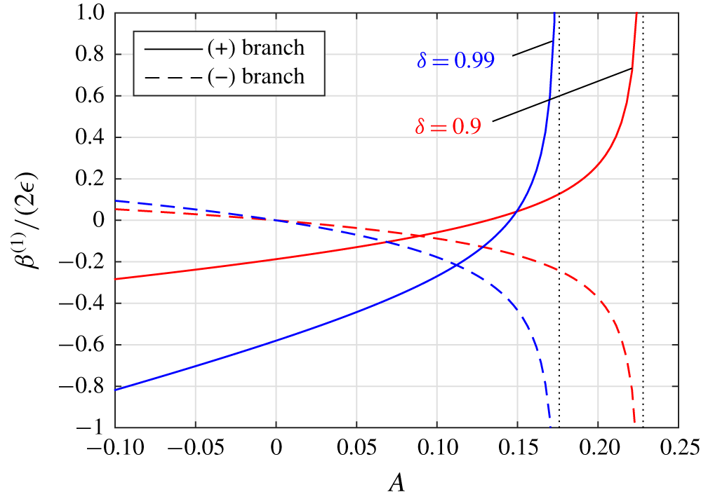
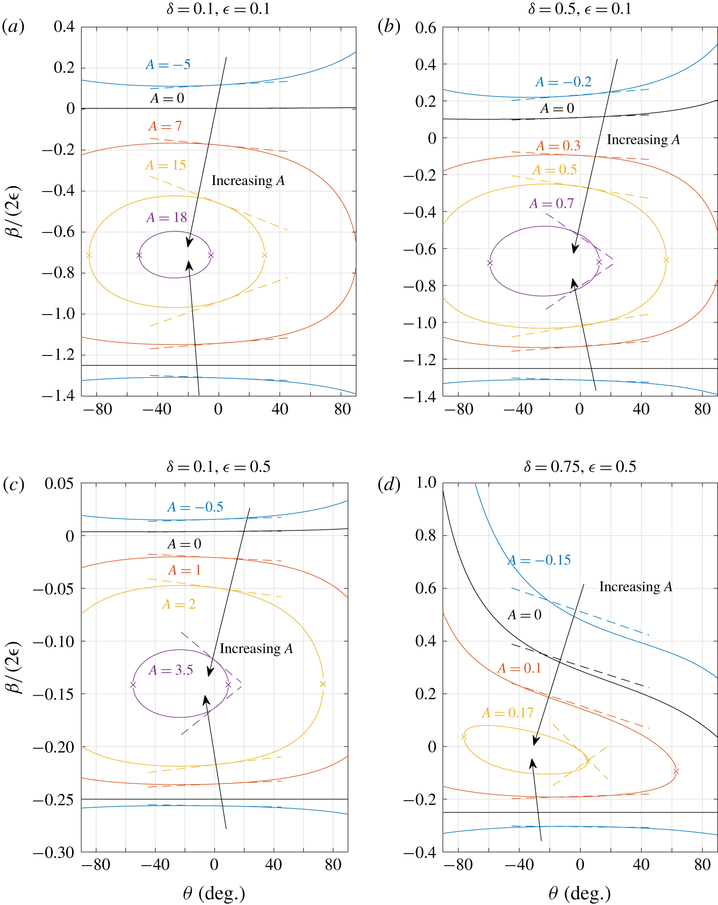
 $A$ is similar to a streamwise Marangoni number, measuring the strength of this feedback mechanism, and its sign is controlled by the direction of the heat flux. For a positive heat flow into the liquid,
 $q_{sl}^{\prime \prime }>0$, then
 $A$ is positive. Assuming
 $Q$ remains positive, this results in a shear stress at the meniscus acting counter to the flow. When
 $q_{sl}^{\prime \prime }<0$, then
 $A<0$ and the shear stress acts in the direction of the flow, increasing the flow rate.
In our analysis we will focus solely on the effect of thermocapillary stress on the hydrodynamic problem. As the thermocapillary stress can be calculated purely from the hydrodynamics, we forgo solving (2.5) for the temperature field (except in the numerical solutions of § 6). Using the formulae in this paper, results for the Nusselt number, and therefore convective resistance, could be calculated by subsequently solving the thermal energy equation (2.5) with negligible transverse advection.
The non-dimensional apparent slip length,  $\unicode[STIX]{x1D6FD}=\unicode[STIX]{x1D6FD}^{\ast }/h^{\ast }$, of a channel flow is defined, following Lauga & Stone (Reference Lauga and Stone2003), by equating the flow rate
 $Q$ with that of an effective one-dimensional Navier slip profile
 $$\begin{eqnarray}w_{NS}=-y^{2}+\frac{y+\unicode[STIX]{x1D6FD}}{1+\unicode[STIX]{x1D6FD}},\quad Q_{NS}=\frac{2}{3}-\frac{1}{2(1+\unicode[STIX]{x1D6FD})},\end{eqnarray}$$
satisfying  $w_{NS}=0$ at
 $y=1$, and the Navier slip condition
 $w_{NS}=\unicode[STIX]{x1D6FD}\,\text{d}w_{NS}/\text{d}y$ at
 $y=0$. An application of the Buckingham pi theorem (Bertrand Reference Bertrand1878) shows that
 $\unicode[STIX]{x1D6FD}$ is a function of eight independent parameter groups,
 $\unicode[STIX]{x1D6FD}=\unicode[STIX]{x1D6FD}(\unicode[STIX]{x1D716},\unicode[STIX]{x1D6FF},\unicode[STIX]{x1D703},Re_{\bot },Ca_{\bot },A,Pr,Br)$, where
 $\unicode[STIX]{x1D716}$,
 $\unicode[STIX]{x1D6FF}$,
 $\unicode[STIX]{x1D703}$,
 $Re_{\bot }$,
 $Ca_{\bot }$ and
 $A$ are as defined above, and the others are the Prandtl number
 $Pr=\unicode[STIX]{x1D707}/(\unicode[STIX]{x1D70C}\unicode[STIX]{x1D6FC})$ and Brinkman number
 $Br=h^{\ast 4}(\unicode[STIX]{x2202}p^{\ast }/\unicode[STIX]{x2202}z^{\ast })^{2}/(4\unicode[STIX]{x1D707}q_{sl}^{\prime \prime }d^{\ast })$. The latter represents viscous dissipation, which we have neglected in the thermal energy equation (2.5). Under the two approximations
 $Re_{\bot }\ll 1$ and
 $Ca_{\bot }\ll 1$, which we make for our asymptotic analysis in § 4, the thermal energy equation becomes irrelevant, and the slip length reduces to a function of only four parameters,
 $\unicode[STIX]{x1D6FD}=\unicode[STIX]{x1D6FD}(\unicode[STIX]{x1D716},\unicode[STIX]{x1D6FF},\unicode[STIX]{x1D703},A)$.
4 Asymptotic solutions of the decoupled streamwise problem
In this section we consider several asymptotic limits of the decoupled streamwise problem (3.10)–(3.14), in particular the limits of small (ridge) period ( $\unicode[STIX]{x1D716}\ll 1$), small meniscus curvature (
 $|\unicode[STIX]{x1D703}|\ll 1$), and small slip fraction (
 $\unicode[STIX]{x1D6FF}\ll 1$) in different combinations. The small period (
 $\unicode[STIX]{x1D716}\ll 1$) will always be taken, so we will consider it first.
4.1 The small period limit ($\unicode[STIX]{x1D716}\ll 1$)

As we have scaled the channel height to unity, the scaled ridge period is given by  $2d^{\ast }/h^{\ast }=2\unicode[STIX]{x1D716}$. Therefore, we refer to the limit
 $\unicode[STIX]{x1D716}\ll 1$ as the small period (compared to channel height) limit, but
 $\unicode[STIX]{x1D716}$ could also be interpreted as the aspect ratio of (half) a period window. Considered in several studies, this limit has been formalised recently in Hodes et al. (Reference Hodes, Kirk, Karamanis and MacLachlan2017) and Kirk (Reference Kirk2018) using matched asymptotics, who demonstrated that remarkable accuracy can be achieved, far outside the small period regime. Corresponding Nusselt number expressions in this limit have also been shown to be accurate (Game et al. Reference Game, Hodes, Kirk and Papageorgiou2018). The domain decomposes into an outer region where
 $y=O(1)$ and the flow is one-dimensional and parabolic, with the periodicity due to the ridges confined to an inner region of height
 $y=O(\unicode[STIX]{x1D716})$.
After rescaling the transverse coordinate  $X=x/\unicode[STIX]{x1D716}$ in (3.10) and searching for an asymptotic solution
 $w=\sum _{n=0}^{\infty }\unicode[STIX]{x1D716}^{n}w_{n}$ with
 $X,y,w_{n}=O(1)$, the solution to all algebraic orders takes the form
 $w=-y^{2}+(y+\unicode[STIX]{x1D716}\hat{\unicode[STIX]{x1D706}})/(1+\unicode[STIX]{x1D716}\hat{\unicode[STIX]{x1D706}})$ where
 $\hat{\unicode[STIX]{x1D706}}=\hat{\unicode[STIX]{x1D706}}(\unicode[STIX]{x1D716})$ is a constant that depends (algebraically) on
 $\unicode[STIX]{x1D716}$. This profile must match with another (inner) solution valid near the ridges, where the solution becomes periodic. The solution
 $w=W(X,Y)$ in the inner region
 $(X,Y)=(x/\unicode[STIX]{x1D716},y/\unicode[STIX]{x1D716})=(O(1),O(1))$ can be related to one for a linear shear flow by the transformation
 $$\begin{eqnarray}W=-\unicode[STIX]{x1D716}^{2}Y^{2}+\frac{\unicode[STIX]{x1D716}}{1+\unicode[STIX]{x1D716}\hat{\unicode[STIX]{x1D706}}}\widehat{W},\end{eqnarray}$$
with  $\widehat{W}$ satisfying
 $$\begin{eqnarray}\displaystyle & \displaystyle \frac{\unicode[STIX]{x2202}^{2}\widehat{W}}{\unicode[STIX]{x2202}X^{2}}+\frac{\unicode[STIX]{x2202}^{2}\widehat{W}}{\unicode[STIX]{x2202}Y^{2}}=0, & \displaystyle\end{eqnarray}$$
 $$\begin{eqnarray}\displaystyle & \displaystyle \widehat{W}=0,\quad \text{on }Y=0,X\notin [-\unicode[STIX]{x1D6FF},\unicode[STIX]{x1D6FF}], & \displaystyle\end{eqnarray}$$
 $$\begin{eqnarray}\displaystyle & \displaystyle \boldsymbol{n}\boldsymbol{\cdot }\unicode[STIX]{x1D735}_{XY}\widehat{W}=[1+\unicode[STIX]{x1D716}\hat{\unicode[STIX]{x1D706}}(\unicode[STIX]{x1D716})]\left[\frac{A}{Q}+\boldsymbol{n}\boldsymbol{\cdot }\unicode[STIX]{x1D735}_{XY}(\unicode[STIX]{x1D716}Y^{2})\right],\quad \text{on the meniscus }S, & \displaystyle\end{eqnarray}$$
 $$\begin{eqnarray}\displaystyle & \displaystyle \widehat{W}\sim Y+\hat{\unicode[STIX]{x1D706}}(\unicode[STIX]{x1D716}),\quad \text{as }Y\rightarrow \infty , & \displaystyle\end{eqnarray}$$
where the last equation, (4.5), is the matching condition with the parabolic outer solution. The undetermined constant has been written in terms of  $\hat{\unicode[STIX]{x1D706}}=O(1)$, the constant term in the far-field condition of
 $\widehat{W}$, which has the appearance of a slip length but does not correspond to the channel flow slip length
 $\unicode[STIX]{x1D6FD}$ as defined in this paper. The effective slip profile is in a rectangular channel, and so the effective slip length
 $\unicode[STIX]{x1D6FD}$ will have contributions from
 $\hat{\unicode[STIX]{x1D706}}$ and from the cross-section being non-rectangular. However, when
 $\unicode[STIX]{x1D716}=0$,
 $\hat{\unicode[STIX]{x1D706}}$ coincides with the slip length of a shear flow over the same surface. There are two distinct forcing terms on the meniscus: the
 $A/Q$ term represents thermocapillary stress, which is an unknown constant, and the remaining term is known explicitly and due to meniscus curvature.
The above formulation accounts for all algebraic orders in  $\unicode[STIX]{x1D716}$, and given a solution for
 $\widehat{W}$, a uniformly valid composite asymptotic solution is simply the inner solution (4.1). We remark that taking the limit
 $\unicode[STIX]{x1D716}\ll 1$ first is most directly relevant to § 4.3, where the small-slip-fraction limit is then taken.
4.2 Small meniscus curvature ($|\unicode[STIX]{x1D703}|\ll 1$), arbitrary slip fraction $\unicode[STIX]{x1D6FF}$


Here we consider small meniscus curvature, i.e. a meniscus close to flat, but valid for any slip fraction  $\unicode[STIX]{x1D6FF}\in [0,1]$. This small curvature limit (
 $|\unicode[STIX]{x1D703}|\ll 1$) can be taken before or after taking
 $\unicode[STIX]{x1D716}\ll 1$, but we do the former as the calculation is simpler. Thus we perform a boundary perturbation on the decoupled streamwise problem (3.10)–(3.14), then take
 $\unicode[STIX]{x1D716}\ll 1$.
The meniscus is a circular arc, and we express its shape in terms of its non-dimensional (signed) curvature, given by  $\unicode[STIX]{x1D705}=\unicode[STIX]{x1D705}^{\ast }d^{\ast }/2=-\sin \unicode[STIX]{x1D703}/(2\unicode[STIX]{x1D6FF})$, the sign chosen so that
 $\unicode[STIX]{x1D705}>0$ corresponds to a downward protruding meniscus. Therefore, for a fixed slip fraction
 $\unicode[STIX]{x1D6FF}$, small meniscus curvature
 $|\unicode[STIX]{x1D705}|\ll 1$ is equivalent to small protrusion angle
 $|\sin \unicode[STIX]{x1D703}|\sim |\unicode[STIX]{x1D703}|\ll 1$. Expansion of the meniscus shape for
 $|\unicode[STIX]{x1D705}|\ll 1$ results in
 $$\begin{eqnarray}Y=-\unicode[STIX]{x1D705}(\unicode[STIX]{x1D6FF}^{2}-X^{2})+O(\unicode[STIX]{x1D705}^{3}),\quad -\unicode[STIX]{x1D6FF}\leqslant X\leqslant \unicode[STIX]{x1D6FF}.\end{eqnarray}$$
Therefore, up to first order in  $\unicode[STIX]{x1D705}$, we can approximate the meniscus deflection as
 $Y=-\unicode[STIX]{x1D705}\unicode[STIX]{x1D702}(X)$ where
 $\unicode[STIX]{x1D702}(X)=\unicode[STIX]{x1D6FF}^{2}-X^{2}$ and perform a regular perturbation expansion in
 $\unicode[STIX]{x1D705}$
 $$\begin{eqnarray}\displaystyle & \displaystyle w=w^{(0)}+\unicode[STIX]{x1D705}w^{(1)}+O(\unicode[STIX]{x1D705}^{2}), & \displaystyle\end{eqnarray}$$
 $$\begin{eqnarray}\displaystyle & \displaystyle Q=Q^{(0)}+\unicode[STIX]{x1D705}Q^{(1)}+O(\unicode[STIX]{x1D705}^{2}), & \displaystyle\end{eqnarray}$$
 $$\begin{eqnarray}\displaystyle & \displaystyle \unicode[STIX]{x1D6FD}=\unicode[STIX]{x1D6FD}^{(0)}+\unicode[STIX]{x1D705}\unicode[STIX]{x1D6FD}^{(1)}+O(\unicode[STIX]{x1D705}^{2}). & \displaystyle\end{eqnarray}$$
In addition, the boundary condition on the meniscus, equation (3.14), is Taylor expanded onto  $y=0$, resulting in a rectangular domain at each order of
 $\unicode[STIX]{x1D705}$, allowing the use of separable series solutions. The relations between the
 $\unicode[STIX]{x1D6FD}^{(i)}$ and
 $Q^{(i)}$ are found by expanding (3.17), giving
 $$\begin{eqnarray}\displaystyle & \displaystyle \unicode[STIX]{x1D6FD}^{(0)}=\frac{1}{2(2/3-Q^{(0)})}-1, & \displaystyle\end{eqnarray}$$
 $$\begin{eqnarray}\displaystyle & \displaystyle \unicode[STIX]{x1D6FD}^{(1)}=2(\unicode[STIX]{x1D6FD}^{(0)}+1)^{2}Q^{(1)}. & \displaystyle\end{eqnarray}$$
4.2.1 Zeroth-order solution, $w^{(0)}$

After substituting the above expansions in  $\unicode[STIX]{x1D705}$ into the decoupled streamwise flow problem (3.10)–(3.14), the resulting problem for
 $w^{(0)}$ is simply the problem for a flat meniscus, given by
 $$\begin{eqnarray}\displaystyle & \displaystyle \unicode[STIX]{x1D6FB}^{2}w^{(0)}=-2,\quad |x|\leqslant \unicode[STIX]{x1D716},0<y<1, & \displaystyle\end{eqnarray}$$
 $$\begin{eqnarray}\displaystyle & \displaystyle w^{(0)}=0,\quad |x|\leqslant \unicode[STIX]{x1D716},y=1, & \displaystyle\end{eqnarray}$$
 $$\begin{eqnarray}\displaystyle & \displaystyle w^{(0)}=0,\quad \unicode[STIX]{x1D6FF}\unicode[STIX]{x1D716}<|x|<\unicode[STIX]{x1D716},y=0, & \displaystyle\end{eqnarray}$$
 $$\begin{eqnarray}\displaystyle & \displaystyle \frac{\unicode[STIX]{x2202}w^{(0)}}{\unicode[STIX]{x2202}y}=\frac{A}{Q^{(0)}},\quad |x|<\unicode[STIX]{x1D716}\unicode[STIX]{x1D6FF},y=0, & \displaystyle\end{eqnarray}$$
with symmetry at  $|x|=\unicode[STIX]{x1D716}$, and solved by Hodes et al. (Reference Hodes, Kirk, Karamanis and MacLachlan2017) (up to scaling differences). A series solution is readily found to be
 $$\begin{eqnarray}w^{(0)}=-y^{2}+y+\unicode[STIX]{x1D716}\tilde{w}^{(0)},\end{eqnarray}$$
where, recalling that  $X=x/\unicode[STIX]{x1D716}$,
 $$\begin{eqnarray}\tilde{w}^{(0)}=(1-y)a_{0}^{(0)}+\mathop{\sum }_{n=1}^{\infty }a_{n}^{(0)}\frac{\text{e}^{-n\unicode[STIX]{x03C0}y/\unicode[STIX]{x1D716}}-\text{e}^{n\unicode[STIX]{x03C0}(y-2)/\unicode[STIX]{x1D716}}}{1-\text{e}^{-2n\unicode[STIX]{x03C0}/\unicode[STIX]{x1D716}}}\cos (n\unicode[STIX]{x03C0}X),\end{eqnarray}$$
and the coefficients  $a_{n}^{(0)}$ are determined by the dual-series equations resulting from the conditions at
 $y=0$
 $$\begin{eqnarray}\displaystyle & \displaystyle a_{0}^{(0)}+\mathop{\sum }_{n=1}^{\infty }a_{n}^{(0)}\cos (n\unicode[STIX]{x03C0}X)=0,\quad \unicode[STIX]{x1D6FF}<|X|<1, & \displaystyle\end{eqnarray}$$
 $$\begin{eqnarray}\displaystyle & \displaystyle \mathop{\sum }_{n=1}^{\infty }a_{n}^{(0)}n\unicode[STIX]{x03C0}\coth \left(\frac{n\unicode[STIX]{x03C0}}{\unicode[STIX]{x1D716}}\right)\cos (n\unicode[STIX]{x03C0}X)=1-\frac{A}{Q^{(0)}}-\unicode[STIX]{x1D716}a_{0}^{(0)},\quad |X|<\unicode[STIX]{x1D6FF}. & \displaystyle\end{eqnarray}$$
These series are for arbitrary  $\unicode[STIX]{x1D716}$ and
 $\unicode[STIX]{x1D6FF}$, but if we now consider the limit of
 $\unicode[STIX]{x1D716}\ll 1$, we see that
 $\coth (n\unicode[STIX]{x03C0}/\unicode[STIX]{x1D716})=1+O(\text{e}^{-2n\unicode[STIX]{x03C0}/\unicode[STIX]{x1D716}})$, and therefore we can approximate
 $\coth (n\unicode[STIX]{x03C0}/\unicode[STIX]{x1D716})\sim 1$ with an exponentially small error. The resulting equations have solution (Sneddon Reference Sneddon1966)
 $$\begin{eqnarray}\displaystyle & \displaystyle a_{0}^{(0)}\sim \frac{(1-A/Q^{(0)})\unicode[STIX]{x1D709}}{1+\unicode[STIX]{x1D716}\unicode[STIX]{x1D709}},\quad \text{where }\unicode[STIX]{x1D709}=\frac{2}{\unicode[STIX]{x03C0}}\log \left[\sec \left(\frac{\unicode[STIX]{x03C0}\unicode[STIX]{x1D6FF}}{2}\right)\right], & \displaystyle\end{eqnarray}$$
 $$\begin{eqnarray}\displaystyle & \displaystyle \tilde{w}^{(0)}(X,0)\sim \frac{1-A/Q^{(0)}}{1+\unicode[STIX]{x1D716}\unicode[STIX]{x1D709}}\frac{2}{\unicode[STIX]{x03C0}}\cosh ^{-1}\left[\frac{\cos \left(\unicode[STIX]{x03C0}X/2\right)}{\cos (\unicode[STIX]{x03C0}\unicode[STIX]{x1D6FF}/2)}\right],\quad |X|<\unicode[STIX]{x1D6FF}, & \displaystyle\end{eqnarray}$$
with flow rate  $Q^{(0)}$ given by
 $$\begin{eqnarray}Q^{(0)}=\frac{1}{6}+\frac{1}{2}\unicode[STIX]{x1D716}a_{0}^{(0)}=\frac{1}{6}+\frac{1}{2}\frac{\unicode[STIX]{x1D716}\unicode[STIX]{x1D709}}{1+\unicode[STIX]{x1D716}\unicode[STIX]{x1D709}}\left(1-\frac{A}{Q^{(0)}}\right).\end{eqnarray}$$
This quadratic equation for  $Q^{(0)}$ gives two roots,
 $$\begin{eqnarray}Q_{\pm }^{(0)}=\frac{1+4\unicode[STIX]{x1D716}\unicode[STIX]{x1D709}}{12(1+\unicode[STIX]{x1D716}\unicode[STIX]{x1D709})}\pm \sqrt{\frac{(1+4\unicode[STIX]{x1D716}\unicode[STIX]{x1D709})^{2}}{144(1+\unicode[STIX]{x1D716}\unicode[STIX]{x1D709})^{2}}-\frac{\unicode[STIX]{x1D716}\unicode[STIX]{x1D709}A}{2(1+\unicode[STIX]{x1D716}\unicode[STIX]{x1D709})}},\end{eqnarray}$$
and formula (4.10) gives correspondingly two solutions for  $\unicode[STIX]{x1D6FD}_{\pm }^{(0)}$,
 $$\begin{eqnarray}\unicode[STIX]{x1D6FD}_{\pm }^{(0)}\sim \frac{(1-A/Q_{\pm }^{(0)})\unicode[STIX]{x1D716}\unicode[STIX]{x1D709}}{1+(A/Q_{\pm }^{(0)})\unicode[STIX]{x1D716}\unicode[STIX]{x1D709}},\quad \unicode[STIX]{x1D716}\ll 1,\end{eqnarray}$$
agreeing with Hodes et al. (Reference Hodes, Kirk, Karamanis and MacLachlan2017), as expected.
4.2.2 First-order solution, $w^{(1)}$

The problem for the first-order correction is given by, along with symmetry at $|x|=\unicode[STIX]{x1D716}$,
 $$\begin{eqnarray}\displaystyle & \displaystyle \unicode[STIX]{x1D6FB}^{2}w^{(1)}=0,\quad |x|\leqslant \unicode[STIX]{x1D716},0<y<1, & \displaystyle\end{eqnarray}$$
 $$\begin{eqnarray}\displaystyle & \displaystyle w^{(1)}=0,\quad |x|\leqslant \unicode[STIX]{x1D716},y=1, & \displaystyle\end{eqnarray}$$
 $$\begin{eqnarray}\displaystyle & \displaystyle w^{(1)}=0,\quad \unicode[STIX]{x1D6FF}\unicode[STIX]{x1D716}<|x|<\unicode[STIX]{x1D716},y=0, & \displaystyle\end{eqnarray}$$
 $$\begin{eqnarray}\displaystyle & \displaystyle \frac{\unicode[STIX]{x2202}w^{(1)}}{\unicode[STIX]{x2202}y}=-\frac{AQ^{(1)}}{(Q^{(0)})^{2}}-\frac{\unicode[STIX]{x2202}}{\unicode[STIX]{x2202}x}\left(\unicode[STIX]{x1D716}\unicode[STIX]{x1D702}\frac{\unicode[STIX]{x2202}w^{(0)}}{\unicode[STIX]{x2202}x}\right)-2\unicode[STIX]{x1D716}\unicode[STIX]{x1D702},\quad |x|<\unicode[STIX]{x1D716}\unicode[STIX]{x1D6FF},y=0, & \displaystyle\end{eqnarray}$$
where (4.12) has been used to simplify the equation on the meniscus (it can be shown that  $w^{(0)}$ indeed satisfies (4.12) there). Similarly to leading order, since the domain is rectangular there is a solution of the form
 $w^{(1)}=\unicode[STIX]{x1D716}\tilde{w}^{(1)}$ with
 $$\begin{eqnarray}\tilde{w}^{(1)}=(1-y)a_{0}^{(1)}+\mathop{\sum }_{n=1}^{\infty }a_{n}^{(1)}\frac{\text{e}^{-n\unicode[STIX]{x03C0}y/\unicode[STIX]{x1D716}}-\text{e}^{n\unicode[STIX]{x03C0}(y-2)/\unicode[STIX]{x1D716}}}{1-\text{e}^{-2n\unicode[STIX]{x03C0}/\unicode[STIX]{x1D716}}}\cos (n\unicode[STIX]{x03C0}X).\end{eqnarray}$$
The coefficients  $a_{n}^{(1)}$ are determined by the dual-series equations that result from enforcing the mixed conditions at
 $y=0$
 $$\begin{eqnarray}\displaystyle & \displaystyle a_{0}^{(1)}+\mathop{\sum }_{n=1}^{\infty }a_{n}^{(1)}\cos (n\unicode[STIX]{x03C0}X)=0,\quad \unicode[STIX]{x1D6FF}<|X|<1, & \displaystyle\end{eqnarray}$$
 $$\begin{eqnarray}\displaystyle & \displaystyle \mathop{\sum }_{n=1}^{\infty }a_{n}^{(1)}n\unicode[STIX]{x03C0}\coth \left(\frac{n\unicode[STIX]{x03C0}}{\unicode[STIX]{x1D716}}\right)\cos (n\unicode[STIX]{x03C0}X)=\frac{AQ^{(1)}}{(Q^{(0)})^{2}}-\unicode[STIX]{x1D716}a_{0}^{(1)}+\frac{\unicode[STIX]{x2202}}{\unicode[STIX]{x2202}X}\left(\unicode[STIX]{x1D702}\frac{\unicode[STIX]{x2202}\tilde{w}^{(0)}}{\unicode[STIX]{x2202}X}\right)+2\unicode[STIX]{x1D716}\unicode[STIX]{x1D702},\quad |X|<\unicode[STIX]{x1D6FF}. & \displaystyle \nonumber\\ \displaystyle & & \displaystyle\end{eqnarray}$$
For arbitrary  $\unicode[STIX]{x1D716}$ these must be solved numerically, but for
 $\unicode[STIX]{x1D716}\ll 1$ we approximate
 $\coth (n\unicode[STIX]{x03C0}/\unicode[STIX]{x1D716})\sim 1$ and the resulting equations can be solved analytically (see (Sneddon Reference Sneddon1966, p. 161) or equations A5–A9 in Sbragaglia & Prosperetti (Reference Sbragaglia and Prosperetti2007)) to give the first coefficient
 $$\begin{eqnarray}a_{0}^{(1)}\sim \frac{1}{1+\unicode[STIX]{x1D716}\unicode[STIX]{x1D709}}\left[\frac{AQ^{(1)}\unicode[STIX]{x1D709}}{(Q^{(0)})^{2}}+\frac{1-A/Q^{(0)}}{1+\unicode[STIX]{x1D716}\unicode[STIX]{x1D709}}L(\unicode[STIX]{x1D6FF})+\unicode[STIX]{x1D716}M(\unicode[STIX]{x1D6FF})\right],\quad \unicode[STIX]{x1D716}\ll 1,\end{eqnarray}$$
where
 $$\begin{eqnarray}\displaystyle & \displaystyle L(\unicode[STIX]{x1D6FF})=-\unicode[STIX]{x1D6FF}^{3}\int _{0}^{1}\frac{[1-\cos (\unicode[STIX]{x1D6FF}\unicode[STIX]{x03C0}s)](1-s^{2})\,\text{d}s}{\cos (\unicode[STIX]{x1D6FF}\unicode[STIX]{x03C0}s)-\cos (\unicode[STIX]{x1D6FF}\unicode[STIX]{x03C0})}, & \displaystyle\end{eqnarray}$$
 $$\begin{eqnarray}\displaystyle & \displaystyle M(\unicode[STIX]{x1D6FF})=2\sqrt{2}\unicode[STIX]{x1D6FF}^{4}\int _{0}^{1}\frac{s(1-s^{2}/3)\sin (\unicode[STIX]{x1D6FF}\unicode[STIX]{x03C0}s/2)\,\text{d}s}{\sqrt{\cos (\unicode[STIX]{x1D6FF}\unicode[STIX]{x03C0}s)-\cos (\unicode[STIX]{x1D6FF}\unicode[STIX]{x03C0})}}. & \displaystyle\end{eqnarray}$$
The flow-rate correction  $Q^{(1)}$ has two contributions, one from the correction to the velocity field itself
 $(Q_{1}^{(1)})$, and one due to the change in cross-sectional area of the domain
 $(Q_{2}^{(1)})$:
 $$\begin{eqnarray}Q^{(1)}=\underbrace{\frac{1}{2\unicode[STIX]{x1D716}}\int _{0}^{1}\!\int _{-\unicode[STIX]{x1D716}}^{\unicode[STIX]{x1D716}}w^{(1)}\,\text{d}x\,\text{d}y}_{Q_{1}^{(1)}}+\underbrace{\frac{1}{2\unicode[STIX]{x1D716}}\int _{-\unicode[STIX]{x1D716}}^{\unicode[STIX]{x1D716}}\unicode[STIX]{x1D716}\unicode[STIX]{x1D702}w^{(0)}(x,0)\,\text{d}x}_{Q_{2}^{(1)}}.\end{eqnarray}$$
From (4.29), we find  $Q_{1}^{(1)}=(1/2)\unicode[STIX]{x1D716}a_{0}^{(1)}$. In the limit
 $\unicode[STIX]{x1D716}\ll 1$, using (4.21) in
 $Q_{2}^{(1)}$ gives
 $$\begin{eqnarray}Q_{2}^{(1)}\sim \frac{1-A/Q^{(0)}}{2(1+\unicode[STIX]{x1D716}\unicode[STIX]{x1D709})}\unicode[STIX]{x1D716}^{2}M(\unicode[STIX]{x1D6FF}),\quad \unicode[STIX]{x1D716}\ll 1.\end{eqnarray}$$
The full expression  $Q^{(1)}=Q_{1}^{(1)}+Q_{2}^{(1)}$ must be rearranged to find
 $Q^{(1)}$ explicitly, using (4.32) and (4.36), giving
 $$\begin{eqnarray}Q^{(1)}\sim \frac{\unicode[STIX]{x1D716}[(1+\unicode[STIX]{x1D716}\unicode[STIX]{x1D709})^{-1}(1-A/Q^{(0)})L(\unicode[STIX]{x1D6FF})+(2-A/Q^{(0)})\unicode[STIX]{x1D716}M(\unicode[STIX]{x1D6FF})]}{2(1+\unicode[STIX]{x1D716}\unicode[STIX]{x1D709})-\unicode[STIX]{x1D716}\unicode[STIX]{x1D709}A/(Q^{(0)})^{2}},\quad \unicode[STIX]{x1D716}\ll 1.\end{eqnarray}$$
This constitutes two corrections, one for each of the two roots for  $Q^{(0)}$. The slip length corrections are then given by (4.11), and the full solution by
 $$\begin{eqnarray}\unicode[STIX]{x1D6FD}=\unicode[STIX]{x1D6FD}^{(0)}+\unicode[STIX]{x1D705}\unicode[STIX]{x1D6FD}^{(1)}+O(\unicode[STIX]{x1D705}^{2})=\unicode[STIX]{x1D6FD}^{(0)}-\frac{\unicode[STIX]{x1D703}}{2\unicode[STIX]{x1D6FF}}\unicode[STIX]{x1D6FD}^{(1)}+O(\unicode[STIX]{x1D703}^{2}).\end{eqnarray}$$
4.2.3 Without thermocapillary stress, $A/Q^{(0)}=0$

If thermocapillary stress is switched off, i.e. we set  $A/Q^{(0)}=0$, the above formulae reduce to
 $$\begin{eqnarray}\displaystyle & \displaystyle \unicode[STIX]{x1D6FD}^{(0)}\sim \unicode[STIX]{x1D716}\unicode[STIX]{x1D709},\quad \unicode[STIX]{x1D716}\ll 1, & \displaystyle\end{eqnarray}$$
 $$\begin{eqnarray}\displaystyle & \displaystyle \unicode[STIX]{x1D6FD}^{(1)}\sim \unicode[STIX]{x1D716}\left[\frac{1}{1+\unicode[STIX]{x1D716}\unicode[STIX]{x1D709}}L(\unicode[STIX]{x1D6FF})+2\unicode[STIX]{x1D716}M(\unicode[STIX]{x1D6FF})\right],\quad \unicode[STIX]{x1D716}\ll 1, & \displaystyle\end{eqnarray}$$
which are extensions of the leading-order formulae of Sbragaglia & Prosperetti (Reference Sbragaglia and Prosperetti2007) to all algebraic orders in  $\unicode[STIX]{x1D716}$ – a significant improvement in accuracy.
4.3 Arbitrary meniscus curvature ($\unicode[STIX]{x1D703}$), small slip fraction ($\unicode[STIX]{x1D6FF}\lesssim 0.75$)


In this section we make no assumption about the size of the meniscus protrusion, instead considering the limit of small slip fraction  $\unicode[STIX]{x1D6FF}$, as in Crowdy (Reference Crowdy2016) and Kirk (Reference Kirk2018). This is in addition to the small period limit,
 $\unicode[STIX]{x1D716}\ll 1$, described in § 4.1, but no further approximation or expansion in
 $\unicode[STIX]{x1D716}$ is made. Therefore, we start from equations (4.2)–(4.5) corresponding to a shear-flow in an inner region close to the ridges. Kirk (Reference Kirk2018) considered the same problem but absent the thermocapillary stress (
 $A/Q$), and therefore we extend their analysis to account for this additional forcing term. We refer to Kirk (Reference Kirk2018) for more details, and here we only present the modified solution.
Since  $\widehat{W}$ is a harmonic function, let
 ${\hat{h}}(z)$ with
 $z=X+\text{i}Y$ be its analytic complex potential such that
 $\widehat{W}=\text{Im}\{{\hat{h}}(z)\}$. If the complex potential for only a single meniscus (with shear stress (4.4)) is
 ${\hat{h}}_{s}(z)$, then the potential for a periodic array of menisci is given approximately by
 $$\begin{eqnarray}\displaystyle & \displaystyle {\hat{h}}_{1}(z)={\hat{h}}_{s}(z)+\hat{\unicode[STIX]{x1D706}}_{1}(\unicode[STIX]{x1D703})\left[\frac{2}{\unicode[STIX]{x03C0}z}-\cot \left(\frac{\unicode[STIX]{x03C0}z}{2}\right)+\frac{\unicode[STIX]{x03C0}}{6}(h_{s}(z)-z)\right], & \displaystyle\end{eqnarray}$$
 $$\begin{eqnarray}\displaystyle & \displaystyle \hat{\unicode[STIX]{x1D706}}_{1}(\unicode[STIX]{x1D703})=\frac{\unicode[STIX]{x1D706}_{1}(\unicode[STIX]{x1D703})-\left[1+{\displaystyle \frac{\unicode[STIX]{x03C0}}{6}}\unicode[STIX]{x1D706}_{1}(\unicode[STIX]{x1D703})\right]\left[{\displaystyle \frac{A}{Q}}\unicode[STIX]{x1D6FF}^{2}J(\unicode[STIX]{x1D703})+\unicode[STIX]{x1D716}\unicode[STIX]{x1D6FF}^{3}I(\unicode[STIX]{x1D703})\right]}{1+\unicode[STIX]{x1D716}\left[1+{\displaystyle \frac{\unicode[STIX]{x03C0}}{6}}\unicode[STIX]{x1D706}_{1}(\unicode[STIX]{x1D703})\right]\left[{\displaystyle \frac{A}{Q}}\unicode[STIX]{x1D6FF}^{2}J(\unicode[STIX]{x1D703})+\unicode[STIX]{x1D716}\unicode[STIX]{x1D6FF}^{3}I(\unicode[STIX]{x1D703})\right]}, & \displaystyle\end{eqnarray}$$
where (Crowdy Reference Crowdy2010, Reference Crowdy2016)
 $$\begin{eqnarray}\displaystyle & \displaystyle h_{s}(z)=\frac{\unicode[STIX]{x1D6FF}}{\unicode[STIX]{x1D6FC}}\frac{4(z/\unicode[STIX]{x1D6FF}-1)^{1/\unicode[STIX]{x1D6FC}}(z/\unicode[STIX]{x1D6FF}+1)^{1/\unicode[STIX]{x1D6FC}}}{(z/\unicode[STIX]{x1D6FF}-1)^{2/\unicode[STIX]{x1D6FC}}-(z/\unicode[STIX]{x1D6FF}+1)^{2/\unicode[STIX]{x1D6FC}}},\quad \unicode[STIX]{x1D6FC}=\frac{2}{\unicode[STIX]{x03C0}}(\unicode[STIX]{x03C0}-\unicode[STIX]{x1D703}), & \displaystyle\end{eqnarray}$$
 $$\begin{eqnarray}\displaystyle & \displaystyle \unicode[STIX]{x1D706}_{1}(\unicode[STIX]{x1D703})=\frac{\unicode[STIX]{x1D6FF}^{2}(3\unicode[STIX]{x03C0}^{3}-4\unicode[STIX]{x03C0}^{2}\unicode[STIX]{x1D703}+2\unicode[STIX]{x03C0}\unicode[STIX]{x1D703}^{2})}{72(\unicode[STIX]{x03C0}-\unicode[STIX]{x1D703})^{2}-\unicode[STIX]{x1D6FF}^{2}\unicode[STIX]{x03C0}(3\unicode[STIX]{x03C0}^{3}-4\unicode[STIX]{x03C0}^{2}\unicode[STIX]{x1D703}+2\unicode[STIX]{x03C0}\unicode[STIX]{x1D703}^{2})}, & \displaystyle\end{eqnarray}$$
 $$\begin{eqnarray}\displaystyle & \displaystyle I(\unicode[STIX]{x1D703})=16\sin \unicode[STIX]{x1D703}\int _{0}^{\unicode[STIX]{x03C0}/2}\frac{\tan ^{2\unicode[STIX]{x1D6FC}}\unicode[STIX]{x1D719}[\cos \unicode[STIX]{x1D703}\tan ^{2\unicode[STIX]{x1D6FC}}\unicode[STIX]{x1D719}+2\tan ^{\unicode[STIX]{x1D6FC}}\unicode[STIX]{x1D719}+\cos \unicode[STIX]{x1D703}]\,\text{d}\unicode[STIX]{x1D719}}{[\tan ^{2\unicode[STIX]{x1D6FC}}\unicode[STIX]{x1D719}+2\cos \unicode[STIX]{x1D703}\tan ^{\unicode[STIX]{x1D6FC}}\unicode[STIX]{x1D719}+1]^{3}}, & \displaystyle\end{eqnarray}$$
 $$\begin{eqnarray}\displaystyle & \displaystyle J(\unicode[STIX]{x1D703})=4\int _{0}^{\unicode[STIX]{x03C0}/2}\frac{\tan ^{\unicode[STIX]{x1D6FC}}\unicode[STIX]{x1D719}\,\text{d}\unicode[STIX]{x1D719}}{\tan ^{2\unicode[STIX]{x1D6FC}}\unicode[STIX]{x1D719}+2\cos \unicode[STIX]{x1D703}\tan ^{\unicode[STIX]{x1D6FC}}\unicode[STIX]{x1D719}+1}. & \displaystyle\end{eqnarray}$$
The subscript ‘1’ is for consistency with Kirk (Reference Kirk2018), where it indicates the asymptotic solution with an error of  $O(\unicode[STIX]{x1D6FF}^{6})$. The potential
 $h_{s}(z)$ is for a single shear-free meniscus (Crowdy Reference Crowdy2010). The thermocapillary stress is indicated in (4.42) by the new term
 $(A/Q)\unicode[STIX]{x1D6FF}^{2}J(\unicode[STIX]{x1D703})$. It also modifies
 ${\hat{h}}_{s}(z)$, which is found by conformally mapping the flow domain to the unit disk and applying the Poisson integral formula – the result is given in appendix A.
We note that the flow rate per unit width,  $Q$, which appears in the above formulae, is still unknown. To calculate
 $Q$ we use a reciprocal result from Green’s second identity in the period cross-section
 $D$, which states that for arbitrary choices
 $\unicode[STIX]{x1D713}$ regular in
 $D$,
 $$\begin{eqnarray}\iint _{D}(w\unicode[STIX]{x1D6FB}^{2}\unicode[STIX]{x1D713}-\unicode[STIX]{x1D713}\unicode[STIX]{x1D6FB}^{2}w)\,\text{d}A=-\oint _{\unicode[STIX]{x2202}D}\left(w\frac{\unicode[STIX]{x2202}\unicode[STIX]{x1D713}}{\unicode[STIX]{x2202}n}-\unicode[STIX]{x1D713}\frac{\unicode[STIX]{x2202}w}{\unicode[STIX]{x2202}n}\right)\text{d}s,\end{eqnarray}$$
where  $\unicode[STIX]{x2202}/\unicode[STIX]{x2202}n$ here is the inward normal derivative. Crowdy (Reference Crowdy2017) has shown previously how use of this identity leads to explicit formulae for the correction to the slip length when the meniscus curvature is small (that prior study did not, however, incorporate thermocapillary stress). In (4.47), choosing
 $w(x,y)$ to be the solution of (3.10)–(3.14) and
 $\unicode[STIX]{x1D713}=(1/2)y^{2}$ results in
 $$\begin{eqnarray}2\unicode[STIX]{x1D716}Q=-\iint _{D}y^{2}\,\text{d}A+\int _{y=1}-\frac{1}{2}\frac{\unicode[STIX]{x2202}w}{\unicode[STIX]{x2202}y}\,\text{d}x+\int _{S}\frac{1}{2}y^{2}\frac{A}{Q}\,\text{d}s-\int _{S}w\frac{\unicode[STIX]{x2202}}{\unicode[STIX]{x2202}n}\left(\frac{1}{2}y^{2}\right)\text{d}s.\end{eqnarray}$$
Note that the third integral is due to thermocapillary stress and can be evaluated exactly. Substituting the outer solution at  $y=1$, the inner solution (4.1) with approximation (4.41) for
 $\unicode[STIX]{x1D6FF}\ll 1$ on
 $S$, this evaluates to
 $$\begin{eqnarray}Q=\overbrace{\frac{2}{3}-\frac{1}{2(1+\unicode[STIX]{x1D716}\hat{\unicode[STIX]{x1D706}})}}^{Q_{outer}}+Q^{\prime },\end{eqnarray}$$
 $$\begin{eqnarray}\displaystyle Q^{\prime } & = & \displaystyle -\frac{\unicode[STIX]{x1D716}^{2}\unicode[STIX]{x1D6FF}^{3}\left[1+{\displaystyle \frac{\unicode[STIX]{x03C0}}{6}}\hat{\unicode[STIX]{x1D706}}_{1}(\unicode[STIX]{x1D703})\right]}{2[1+\unicode[STIX]{x1D716}\hat{\unicode[STIX]{x1D706}}(\unicode[STIX]{x1D703})]}I(\unicode[STIX]{x1D703})+\frac{A}{2Q}\unicode[STIX]{x1D716}^{2}\unicode[STIX]{x1D6FF}^{3}[F_{1}(\unicode[STIX]{x1D703})-G_{1}(\unicode[STIX]{x1D703})]\nonumber\\ \displaystyle & & \displaystyle +\,\frac{1}{2}\unicode[STIX]{x1D716}^{3}\unicode[STIX]{x1D6FF}^{4}[F_{2}(\unicode[STIX]{x1D703})-G_{2}(\unicode[STIX]{x1D703})]+O(\unicode[STIX]{x1D6FF}^{7}),\nonumber\end{eqnarray}$$
where  $Q_{outer}$ is the flow rate of the outer slip profile down to
 $y=0$, and
 $Q^{\prime }$ the extra contribution from the change in boundary shape, with
 $$\begin{eqnarray}\displaystyle & \displaystyle F_{1}(\unicode[STIX]{x1D703})={\textstyle \frac{1}{2}}\csc ^{3}\unicode[STIX]{x1D703}\left[\unicode[STIX]{x1D703}(2+\cos 2\unicode[STIX]{x1D703})-{\textstyle \frac{3}{2}}\sin 2\unicode[STIX]{x1D703}\right], & \displaystyle\end{eqnarray}$$
 $$\begin{eqnarray}\displaystyle & \displaystyle F_{2}(\unicode[STIX]{x1D703})=\csc ^{4}\unicode[STIX]{x1D703}\left[\unicode[STIX]{x1D703}(3+2\cos 2\unicode[STIX]{x1D703})-{\textstyle \frac{7}{3}}\sin 2\unicode[STIX]{x1D703}-{\textstyle \frac{1}{12}}\sin 4\unicode[STIX]{x1D703}\right], & \displaystyle\end{eqnarray}$$
and  $G_{1}(\unicode[STIX]{x1D703})$ and
 $G_{2}(\unicode[STIX]{x1D703})$ are given explicitly in appendix B.
We remark that  $\hat{\unicode[STIX]{x1D706}}(\unicode[STIX]{x1D703})$ and
 $Q^{\prime }$ depend on
 $Q$ itself therefore (4.49) implicitly determines
 $Q$. Remarkably, substituting the approximation (4.42) for
 $\hat{\unicode[STIX]{x1D706}}(\unicode[STIX]{x1D703})$ into (4.49) still leads to a quadratic equation for
 $Q$, roots given by
 $$\begin{eqnarray}Q^{\pm }(\unicode[STIX]{x1D703})=\frac{b(\unicode[STIX]{x1D703})}{2}\pm \sqrt{\frac{b(\unicode[STIX]{x1D703})^{2}}{4}-Ac(\unicode[STIX]{x1D703})},\end{eqnarray}$$
where
 $$\begin{eqnarray}\displaystyle b(\unicode[STIX]{x1D703}) & = & \displaystyle -\frac{1+\unicode[STIX]{x1D716}^{2}\unicode[STIX]{x1D6FF}^{3}I(\unicode[STIX]{x1D703})\left[1+{\displaystyle \frac{\unicode[STIX]{x03C0}}{6}}\unicode[STIX]{x1D706}_{1}(\unicode[STIX]{x1D703})\right]\left[2+\left(\unicode[STIX]{x1D716}-{\displaystyle \frac{\unicode[STIX]{x03C0}}{6}}\right)\unicode[STIX]{x1D716}\unicode[STIX]{x1D6FF}^{3}I(\unicode[STIX]{x1D703})\right]}{2[1+\unicode[STIX]{x1D716}\unicode[STIX]{x1D706}_{1}(\unicode[STIX]{x1D703})]}\nonumber\\ \displaystyle & & \displaystyle +\,\frac{2}{3}+\frac{1}{2}\unicode[STIX]{x1D716}^{3}\unicode[STIX]{x1D6FF}^{4}[F_{2}(\unicode[STIX]{x1D703})-G_{2}(\unicode[STIX]{x1D703})],\end{eqnarray}$$
 $$\begin{eqnarray}\displaystyle c(\unicode[STIX]{x1D703}) & = & \displaystyle \frac{\unicode[STIX]{x1D716}\unicode[STIX]{x1D6FF}^{2}J(\unicode[STIX]{x1D703})\left[1+{\displaystyle \frac{\unicode[STIX]{x03C0}}{6}}\unicode[STIX]{x1D706}_{1}(\unicode[STIX]{x1D703})\right]\left[1+\left(\unicode[STIX]{x1D716}-{\displaystyle \frac{\unicode[STIX]{x03C0}}{6}}\right)\unicode[STIX]{x1D716}\unicode[STIX]{x1D6FF}^{3}I(\unicode[STIX]{x1D703})\right]}{2[1+\unicode[STIX]{x1D716}\unicode[STIX]{x1D706}_{1}(\unicode[STIX]{x1D703})]}\nonumber\\ \displaystyle & & \displaystyle -\,\frac{1}{2}\unicode[STIX]{x1D716}^{2}\unicode[STIX]{x1D6FF}^{3}[F_{1}(\unicode[STIX]{x1D703})-G_{1}(\unicode[STIX]{x1D703})].\end{eqnarray}$$
Finally, equating (3.17) and (4.52), the two solutions for the channel flow slip lengths are given by
 $$\begin{eqnarray}\unicode[STIX]{x1D6FD}^{\pm }(\unicode[STIX]{x1D703})=\frac{-1+3b(\unicode[STIX]{x1D703})\pm 3\sqrt{b(\unicode[STIX]{x1D703})^{2}-4Ac(\unicode[STIX]{x1D703})}}{+4-3b(\unicode[STIX]{x1D703})\mp 3\sqrt{b(\unicode[STIX]{x1D703})^{2}-4Ac(\unicode[STIX]{x1D703})}}.\end{eqnarray}$$
This is the main result of this section. The formula is explicit, valid with no restriction on angle  $\unicode[STIX]{x1D703}$ or
 $A$, and given in terms of the well-behaved functions
 $\unicode[STIX]{x1D706}_{1}(\unicode[STIX]{x1D703})$,
 $I(\unicode[STIX]{x1D703})$,
 $J(\unicode[STIX]{x1D703})$,
 $F_{1}(\unicode[STIX]{x1D703})$,
 $G_{1}(\unicode[STIX]{x1D703})$,
 $F_{2}(\unicode[STIX]{x1D703})$ and
 $G_{2}(\unicode[STIX]{x1D703})$. Both solutions are real if
 $b(\unicode[STIX]{x1D703})^{2}-4Ac(\unicode[STIX]{x1D703})\geqslant 0$ (notice that
 $b(\unicode[STIX]{x1D703})$ and
 $c(\unicode[STIX]{x1D703})$ are independent of
 $A$). The sign of
 $c(\unicode[STIX]{x1D703})$ is not obvious but we numerically observe it to always be positive, implying the upper bound
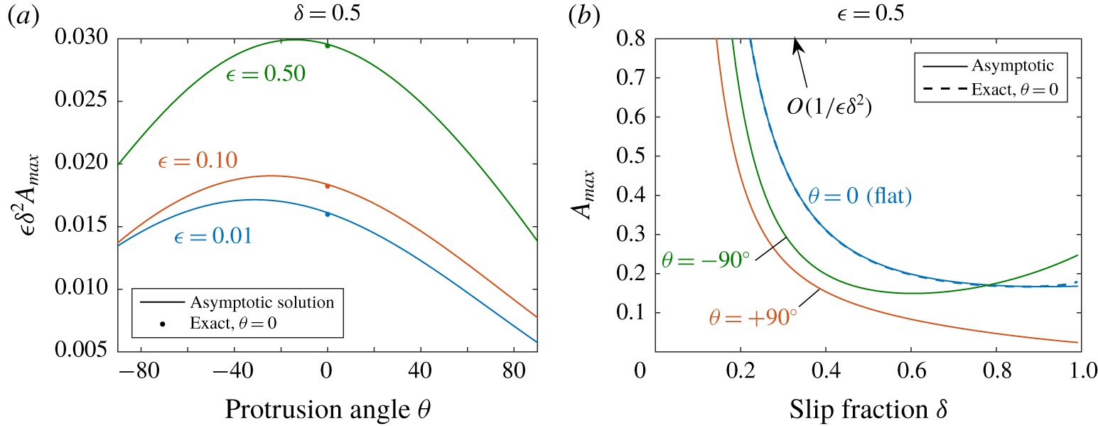
 $A\leqslant A_{max}\sim b(\unicode[STIX]{x1D703})^{2}/[4c(\unicode[STIX]{x1D703})]$ for real solutions. Taking the limit of negligible thermocapillary stress,
 $A\rightarrow 0$, the (+) solution reduces to the hydrodynamic solution in Kirk (Reference Kirk2018), where
 $F_{2}(\unicode[STIX]{x1D703})$ and
 $G_{2}(\unicode[STIX]{x1D703})$ correspond to
 $F(\unicode[STIX]{x1D703})$ and
 $G(\unicode[STIX]{x1D703})$, respectively. Here, the quantities
 $F_{1}(\unicode[STIX]{x1D703})$,
 $G_{1}(\unicode[STIX]{x1D703})$ and
 $J(\unicode[STIX]{x1D703})$ are entirely new, however.
The two limits  $\unicode[STIX]{x1D716}\ll 1$ and
 $\unicode[STIX]{x1D6FF}\ll 1$ were taken to derive (4.55), but we expect it to have an extended range of validity, i.e. up to
 $\unicode[STIX]{x1D716}\lesssim 1$ and
 $\unicode[STIX]{x1D6FF}\lesssim 0.75$ with ≲5 % relative error. Setting
 $\unicode[STIX]{x1D703}=0$, the above formulae for
 $\unicode[STIX]{x1D6FD}^{\pm }(0)$ and
 $Q^{\pm }(0)$ reduce exactly (up to
 $O(\unicode[STIX]{x1D6FF}^{6})$) to those for a flat meniscus given earlier ((4.24) and (4.23)) with the quantity
 $\unicode[STIX]{x1D709}=(2/\unicode[STIX]{x03C0})\log [\sec (\unicode[STIX]{x1D6FF}\unicode[STIX]{x03C0}/2)]$ substituted with
 $\unicode[STIX]{x1D706}_{1}=(\unicode[STIX]{x03C0}/4)\unicode[STIX]{x1D6FF}^{2}/(1-(\unicode[STIX]{x03C0}^{2}/24)\unicode[STIX]{x1D6FF}^{2})$, which differ by only
 $O(\unicode[STIX]{x1D6FF}^{6})$.
5 Results and discussion
In this section we present the effect of the thermocapillary stress, its strength measured by  $A$, on the slip length
 $\unicode[STIX]{x1D6FD}$ and velocity field when the meniscus is curved, as calculated by the asymptotic formulae (4.38) and (4.55). In each asymptotic case considered, when heat transfer is present and thermocapillary stress is included, the shear stress
 $A/Q$ becomes a function of the solution, and therefore
 $Q$ becomes a function of itself, i.e.
 $Q=Q(\unicode[STIX]{x1D716},\unicode[STIX]{x1D6FF},\unicode[STIX]{x1D703},A/Q)$. This results in a quadratic equation for
 $Q$, and therefore two possible solutions,
 $Q^{\pm }$, for each parameter set. Consequently, there are two possible flow fields
 $w^{\pm }$ and slip lengths
 $\unicode[STIX]{x1D6FD}^{\pm }(\unicode[STIX]{x1D703})$, for any value of the parameters
 $\unicode[STIX]{x1D716}$,
 $\unicode[STIX]{x1D6FF}$ or
 $\unicode[STIX]{x1D703}$. It is likely that only the (+) solution is physically relevant – see the discussion on p. 319 of Hodes et al. (Reference Hodes, Kirk, Karamanis and MacLachlan2017).
5.1 Effect of small meniscus curvature
To see the effect of perturbing the meniscus from flat when thermocapillary stress is present, we can study the first correction  $-\unicode[STIX]{x1D703}\unicode[STIX]{x1D6FD}^{(1)}/(2\unicode[STIX]{x1D6FF})$ (see (4.38)) to the slip length for
 $|\unicode[STIX]{x1D703}|\ll 1$, given by (4.11), (4.37). The coefficient
 $\unicode[STIX]{x1D6FD}^{(1)}$ is shown in figure 2 against
 $A$. We will focus on the physically relevant (+) solution branch but the (-) solution is included for completeness. Recall that
 $A>0$ corresponds to a positive heat flux into the domain, i.e. heating of the liquid, and
 $A<0$ corresponds to a negative heat flux, i.e. cooling of the liquid.
Correction to the slip length,  $\unicode[STIX]{x1D6FD}^{(1)}/(2\unicode[STIX]{x1D716})$, due to small meniscus curvature,
 $|\unicode[STIX]{x1D703}|\ll 1$, against
 $A$. Both (±) solution branches are shown, with (+) the physical solution. Range of
 $A$ is
 $-0.1<A<A_{max}|_{\unicode[STIX]{x1D703}=0}$, with
 $A_{max}|_{\unicode[STIX]{x1D703}=0}=(1+4\unicode[STIX]{x1D716}\unicode[STIX]{x1D709})^{2}/[72\unicode[STIX]{x1D716}\unicode[STIX]{x1D709}(1+\unicode[STIX]{x1D716}\unicode[STIX]{x1D709})]$ the value when the roots become complex in (4.23).
 $\unicode[STIX]{x1D716}=0.5$.

Typically  $\unicode[STIX]{x1D6FD}^{(1)}<0$ for
 $A=0$, i.e. no heating or thermocapillary stress, meaning slip is increased (the exception is when the ridge period is larger than the channel height (
 $\unicode[STIX]{x1D716}\gtrsim 1$) and the change in cross-sectional area becomes more important, resulting in the opposite behaviour) for positive protrusion
 $\unicode[STIX]{x1D703}>0$ (and decreased for negative protrusion
 $\unicode[STIX]{x1D703}<0$). This is because the shear-free meniscus is being moved closer to the centre of the channel. Increasing
 $A$ sufficiently from zero (i.e. heating) causes
 $\unicode[STIX]{x1D6FD}^{(1)}$ to change sign to
 $\unicode[STIX]{x1D6FD}^{(1)}>0$, and the behaviour is reversed: slip is decreased for positive protrusion
 $\unicode[STIX]{x1D703}>0$ (and vice versa for
 $\unicode[STIX]{x1D703}<0$). This is because the induced shear stress eventually becomes large enough – in fact larger than the stress on the solid ridge – that moving the meniscus towards the centre of the channel becomes a detriment rather than enhancement to the flow. And this transition always occurs for large enough
 $A$, until eventually
 $\unicode[STIX]{x1D6FD}^{(1)}\rightarrow +\infty$ and the small curvature expansion breaks down as
 $A\rightarrow A_{max}|_{\unicode[STIX]{x1D703}=0}$, the value when the roots become complex. This is discussed further in the next section.
5.2 Arbitrary meniscus curvature
Plotted in figure 3 for various positive and negative values of  $A$ is the slip length normalised by the ridge period,
 $\unicode[STIX]{x1D6FD}/(2\unicode[STIX]{x1D716})$, over the whole range of
 $\unicode[STIX]{x1D703}\in [-\unicode[STIX]{x03C0}/2,\unicode[STIX]{x03C0}/2]$. The solid and dashed lines are the formulae (4.55) and (4.38) for
 $\unicode[STIX]{x1D6FF}\ll 1$ and for
 $|\unicode[STIX]{x1D703}|\ll 1$, respectively. When
 $A=0$, despite there being two solutions in (4.55), only the (+) solution (the upper branch in figure 3) corresponds to the case where heat transfer is absent,
 $A/Q^{+}=0$, in Kirk (Reference Kirk2018). The (-) solution has (see (4.52)) a vanishing flow rate
 $Q^{-}\rightarrow 0$ as
 $A\rightarrow 0$, with a non-zero shear stress
 $A/Q^{-}\rightarrow b(\unicode[STIX]{x1D703})/c(\unicode[STIX]{x1D703})>0$, which has no physical interpretation and can likely be ignored. The (-) branch is likely to be temporally unstable, but such a determination would need full time-dependent simulations of the coupled hydrodynamic and thermal problems, which is a considerable computational task outside the scope of this paper.
Slip length normalised by the period ( $2\unicode[STIX]{x1D716}$) against protrusion angle for arbitrary angles (4.55) (solid lines) and small angles (4.38) (dashed lines), for various values of the thermocapillary parameter
 $A$, with
 $A>0$ and
 $A<0$ denoting heating and cooling of the liquid, respectively. Upper/lower branches are using the (+)/(-) solutions. Crosses denote saddle-node bifurcation points, beyond which the solutions are complex.

For any set of parameters, and indeed any angle  $\unicode[STIX]{x1D703}$, as
 $A$ is increased the (+) solution decreases (a reduction of slip) until it eventually meets the (-) solution at a saddle-node bifurcation (denoted by a cross) and the solutions become complex. This occurs at the critical value
 $A_{max}=b^{2}/(4c)$, above which (
 $A>A_{max}$) there are no real solutions. Contrary to this behaviour, if
 $A<0$ the (+) solution is increased (an enhancement of slip), with a solution for all parameters. Large angles are most sensitive to an increase in heat flux, with large positive angles transitioning before large negative ones. The range of
 $\unicode[STIX]{x1D703}$ for which real solutions exist,
 $[\unicode[STIX]{x1D703}_{-},\unicode[STIX]{x1D703}_{+}]$ say, shrinks in size and eventually vanishes for
 $A$ large enough, leaving no real solutions for any angle
 $\unicode[STIX]{x1D703}$. This is shown clearly by figure 4 where the maximum value of
 $A$ for real solutions,
 $A_{max}$, is plotted versus
 $\unicode[STIX]{x1D703}$ and slip fraction
 $\unicode[STIX]{x1D6FF}$. There is good agreement with the exact value for a flat meniscus (
 $\unicode[STIX]{x1D703}=0$), but we remark that
 $A_{max}$ for the small
 $\unicode[STIX]{x1D703}$ expansion originates from the leading-order (flat) solution so coincides with the case
 $\unicode[STIX]{x1D703}=0$. Figure 4(a) shows that transition occurs for large positive angles first, and moderate negative angles last (-40° ≲𝜃≲-20°). Large negative angles are not last, as one might expect from the arguments for small angles at the end of § 5.1, and we conclude that the additional meniscus surface area for the thermocapillary stress to act over eventually outweighs the effect of moving the boundary further from the channel centre. The same behaviour is seen for all channel geometries examined, in the range
 $\unicode[STIX]{x1D716},\unicode[STIX]{x1D6FF}\leqslant 1$. From (4.53) and (4.54), to leading order
 $A_{max}=O(1/(\unicode[STIX]{x1D716}\unicode[STIX]{x1D6FF}^{2}))$ as
 $\unicode[STIX]{x1D716}\rightarrow 0$ or
 $\unicode[STIX]{x1D6FF}\rightarrow 0$ (see figure 4b), so for a vanishing ridge period or slip fraction, the menisci vanish and there is always a real solution.
The critical value  $A_{max}$, where real solutions exist for
 $A\leqslant A_{max}$ and none for
 $A>A_{max}$. Solid lines are using
 $A_{max}\sim b^{2}/(4c)$ for
 $\unicode[STIX]{x1D6FF}\ll 1$, and dots or dashes are using the exact solution (Hodes et al. Reference Hodes, Kirk, Karamanis and MacLachlan2017) for
 $\unicode[STIX]{x1D703}=0$ (flat). We plot
 $\unicode[STIX]{x1D716}\unicode[STIX]{x1D6FF}^{2}A_{max}=O(1)$ in (a) for clarity.

For a slip fraction of  $\unicode[STIX]{x1D6FF}=0.75$ (figure 3d), even though the asymptotic solution for
 $\unicode[STIX]{x1D6FF}\ll 1$ may have an error of 5 % or more, the qualitative behaviour is corroborated by the small curvature solutions (dashed lines) which apply with no restriction on
 $\unicode[STIX]{x1D6FF}$. In general, figure 3 shows that the small curvature approximation is good up to ±π/6 (or ±30°) except when
 $A$ approaches
 $A_{max}$ for
 $\unicode[STIX]{x1D703}=0$ and the gradients become large (no small curvature approximation is plotted for
 $A=18$ in 3(a) as the leading-order solution is not real). This also explains the breakdown of the small curvature expansion, i.e. the reason
 $\unicode[STIX]{x1D6FD}^{(1)}$ is singular as
 $A\rightarrow A_{max}|_{\unicode[STIX]{x1D703}=0}$.
The case of no real solutions for some parameter values is a surprising result, but it only implies that there are no solutions satisfying the assumptions and approximations we made in this paper, chiefly, that the flow and temperature is steady, fully developed, with  $Re_{\bot }\ll 1$ and
 $Ca_{\bot }\ll 1$, and satisfies an isoflux boundary condition on the ridge tips. No solutions under these conditions implies at least one condition must be relaxed for a solution to be found. The numerical solutions in § 6, when
 $Re_{\bot }$ is arbitrary, failed to converge if
 $A$ was sufficiently large (above approximately
 $A_{max}$), suggesting the same behaviour is present when the flow and temperature are fully coupled. We hypothesise that the behaviour is due to the particular form of the streamwise shear-stress condition,
 $\unicode[STIX]{x2202}w/\unicode[STIX]{x2202}n=A/Q$. This is due to the exact evaluation of the streamwise temperature gradient
 $\unicode[STIX]{x2202}T/\unicode[STIX]{x2202}z$ being a constant depending on
 $Q$, equation (2.11), which is only the case if the steady-state, fully developed and isoflux conditions are met. As the isoflux condition can always be imposed in practice, this leaves two possibilities: (i) the solution is not steady, i.e. it is time dependent and we have found a novel criterion for temporal instability; or (ii) the solution is steady but three-dimensional, and the fully developed assumptions (where the temperature increases linearly with
 $z$) cannot hold, even with a doubly infinite channel. To distinguish between these possibilities, we anticipate that a full time-dependent solution of the coupled hydrodynamic and thermal equations in three dimensions is necessary, which is outside the scope of this work.
6 Numerical solutions of the coupled problem
6.1 Numerical method
The full steady problem of § 2, consisting of the continuity, Navier–Stokes and thermal energy equations, was solved using ANSYS FLUENT, a commercial computational fluid dynamics finite volume software package, with the viscous dissipation terms in the thermal energy equation switched off. The meniscus was also assumed to be a circular arc (therefore assuming  $Ca_{\bot }\ll 1$) so that its shape did not have to be determined as part of the solution. The computational domain corresponded to half of one period,
 $0<x^{\ast }<d^{\ast }$ (with mirror symmetry at
 $x^{\ast }=0,d^{\ast }$), but necessarily had a finite streamwise length
 $\unicode[STIX]{x0394}z^{\ast }$ due to the structure of FLUENT requiring a three-dimensional domain. Conditions of hydrodynamically and thermally developed flow were therefore imposed via a translational periodic boundary condition in the streamwise direction (Patankar, Liu & Sparrow Reference Patankar, Liu and Sparrow1977) between
 $z^{\ast }=0$ and
 $z^{\ast }=\unicode[STIX]{x0394}z^{\ast }$, where the temperature and pressure were separated into linear and periodic components in
 $z^{\ast }$, the periodic part vanishing upon convergence.
The equations were discretised using a second-order upwind scheme and, because the velocity and temperature fields are coupled, they were computed iteratively. At a given iteration, the thermocapillary stress along the meniscus was calculated and, subsequently, the continuity equation and the Navier–Stokes equations were solved using the pressure-based coupled solver, updating the velocity field. Next, the temperature was updated by solving the thermal energy equation. These steps were repeated sequentially until convergence.
The model was initially executed on a uniform structured spatial mesh. Then, the mesh was refined based on the gradient and boundary adaptation procedures in FLUENT and the model was executed again. The process was repeated multiple times until the calculated value of  $Q$ changed by less than 1 %. This was accomplished after refining the mess typically three times. The mesh refinement was case dependent, but the final number of control volumes for each case was always greater than 4 million.
6.2 Results and comparison with solutions for $Re_{\bot }\ll 1$

For several channel geometries, simulations were performed for a variety of transverse Reynolds numbers  $Re_{\bot }$ to assess the validity of the Stoke flow solutions as
 $Re_{\bot }\rightarrow 0$. The thermophysical parameters used were the same as those in Hodes et al. (Reference Hodes, Kirk, Karamanis and MacLachlan2017) for Galinstan with a channel height of
 $h^{\ast }=40~\unicode[STIX]{x03BC}\text{m}$ and (half) ridge period
 $d^{\ast }=10~\unicode[STIX]{x03BC}\text{m}$, resulting in non-dimensional parameter values
 $Pr=0.043$,
 $\unicode[STIX]{x1D716}=0.25$,
 $A=0.0580$ and
 $Re_{\bot }=1.52\times 10^{2}$ (the differences from Hodes et al. (Reference Hodes, Kirk, Karamanis and MacLachlan2017) are due to slight differences in non-dimensional definitions).
To compare with the asymptotic solutions, which make further assumptions on the protrusion angle  $\unicode[STIX]{x1D703}$ and slip fraction
 $\unicode[STIX]{x1D6FF}$, the following cases were considered: (i) 𝜃 = ±20. 1° with
 $\unicode[STIX]{x1D6FF}=0.975$ (small angle regime); (ii)
 $\unicode[STIX]{x1D703}=\pm 90^{\circ }$ with
 $\unicode[STIX]{x1D6FF}=0.5$ (small slip fraction regime); (iii)
 $\unicode[STIX]{x1D703}=\pm 56.9^{\circ }$ with
 $\unicode[STIX]{x1D6FF}=0.975$ (large angle and slip fraction). Here
 $\unicode[STIX]{x1D703}=-56.9^{\circ }$ is the largest possible negative protrusion angle for Galinstan on Teflon while remaining in the Cassie state, and 𝜃 = -20. 1° is the corresponding angle for water (Liu et al. Reference Liu, Sen and Kim2012). For each of these cases, simulations were performed for five values of
 $Re_{\bot }$ given by 1. 52 × 10-1, 1. 52 × 100, 1. 52 × 101, 1. 52 × 102, 1. 52 × 103, and the slip lengths
 $\unicode[STIX]{x1D6FD}$ are shown in figure 5. The results tend to the corresponding asymptotic solution for
 $Re_{\bot }$ in cases (i) and (ii) as
 $Re_{\bot }$ decreases, with only the small residual error remaining due to the small angle (
 $|\unicode[STIX]{x1D703}|\ll 1$) or slip fraction approximations (
 $\unicode[STIX]{x1D6FF}\ll 1$). See table 1 for the maximum relative errors at the lowest value of
 $Re_{\bot }$. In case (i), the error of the small angle approximation is ⩽2.7 %, and in case (ii) the error of the dilute packing formula is ⩽1.9 %, but in case (iii), where we expect neither to be accurate, the error of both is >10 %. (The fact the error of the small angle solution is the very small value of 0.14 % for
 $\unicode[STIX]{x1D703}=-90^{\circ }$ is coincidental.) For all cases, accounting for inertial effects decreases the slip length, as seen for flat menisci (Hodes et al. Reference Hodes, Kirk, Karamanis and MacLachlan2017), but this decrease is largest for negative protrusion angles.
The slip length  $\unicode[STIX]{x1D6FD}$ from the numerical computations in FLUENT as
 $Re_{\bot }$ is varied. The asymptotic solutions for
 $|\unicode[STIX]{x1D703}|\ll 1$ (4.38) and
 $\unicode[STIX]{x1D6FF}\ll 1$ (4.55) are the horizontal solid and dashed lines, respectively, and are valid for sufficiently small
 $Re_{\bot }$. The colour red (blue) indicates positive (negative)
 $\unicode[STIX]{x1D703}$.

Maximum relative error (%) in slip length  $\unicode[STIX]{x1D6FD}$ between asymptotic solutions for
 $Re_{\bot }\ll 1$ and full numerical simulations at
 $Re_{\bot }=1.52\times 10^{-1}$. Small angle
 $|\unicode[STIX]{x1D703}|\ll 1$ and dilute packing
 $\unicode[STIX]{x1D6FF}\ll 1$ given by (4.38) and (4.55), respectively.

In case (iii), where  $\unicode[STIX]{x1D703}=\pm 56.9^{\circ }$ and
 $\unicode[STIX]{x1D6FF}=0.975$, both of the asymptotic solutions should be invalid, thus we plot the numerical three-dimensional velocity field in figures 6 and 7 for non-negligible inertia (
 $Re_{\bot }=1.52\times 10^{2}$). The transverse velocity field shows a pair of counter-rotating vortices that are driven by the transverse thermocapillary stresses.
Non-dimensional streamwise velocity field from FLUENT simulations of the full coupled problem when inertia is not negligible ( $Re_{\bot }=1.52\times 10^{2}$), and with protrusion angles (left to right)
 $\unicode[STIX]{x1D703}=-56.9^{\circ }$, 0, +56. 9°.

Non-dimensional transverse velocity field from FLUENT simulations of the full coupled problem when inertia is not negligible ( $Re_{\bot }=1.52\times 10^{2}$), and with protrusion angles (left to right)
 $\unicode[STIX]{x1D703}=-56.9^{\circ }$, 0, +56. 9°.

7 Conclusions
Pressure-driven flow in the presence of heat transfer through a microchannel patterned with isoflux longitudinal ridges (on one or both walls) has been considered in detail, simultaneously accounting for curvature and thermocapillary stress at the menisci. The temperature variation at the menisci influences the streamwise flow, but also creates a transverse cell flow. Under the assumption that Reynolds number based on the transverse flow is small, the streamwise flow decouples from the transverse, with only the streamwise thermocapillary stress retained. This resulting problem for the streamwise flow is characterised by three geometric parameters ( $\unicode[STIX]{x1D716},\unicode[STIX]{x1D6FF},\unicode[STIX]{x1D703}$) and a parameter (
 $A$) describing the strength (and direction relative to the imposed pressure gradient) of the thermocapillary stress.
To analyse and quantify the combined influence of thermocapillary stress and meniscus curvature on the apparent slip length, we employed several asymptotic limits, each previously proven to give accurate explicit solutions with very wide ranges of validity. The main approach relied on a matched asymptotic expansion in the small-ridge-period limit ( $\unicode[STIX]{x1D716}\ll 1$), reducing the problem to that of a shear-driven flow close to the ridges with exponentially small errors. In addition to this limit, two different further limits were taken: (i) small meniscus curvature
 $|\unicode[STIX]{x1D703}|\ll 1$ (close to flat) using boundary perturbation; and (ii) arbitrarily curved menisci but with small slip or cavity fraction
 $\unicode[STIX]{x1D6FF}\ll 1$. These limits are complementary and, to the orders presented here, we expect them to be good approximations up to
 $|\unicode[STIX]{x1D703}|\lesssim 40^{\circ }$ and
 $\unicode[STIX]{x1D6FF}\lesssim 0.75$, respectively, covering much of the parameter space. To complete the parameter space, the dense meniscus packing limit of
 $1-\unicode[STIX]{x1D6FF}\ll 1$ with arbitrary angles is one possibility, where the approach of Schnitzer (Reference Schnitzer2017) may be useful (albeit only for positive protrusion angles).
For each solution presented, the thermocapillary stress depends on the resultant flow rate, giving a constraint on the flow rate in the form of a quadratic equation. Consequently, for each choice of parameters, there are up to two solutions (only one of which is physically relevant) for the flow rate, flow field and slip length. For a positive heat flux (heating), the shear stress acts against the flow and slip is reduced for any meniscus shape, until a saddle-node bifurcation after which there are no more real solutions. Curving the meniscus up into the liquid and down out of the liquid amounts to moving the meniscus shear-stress condition closer to and away from the liquid bulk, respectively. When the curvature is small, we found that if the shear stress is large enough (at least as large as the shear stress on the ridge), a protrusion into (out of) the liquid reduces (enhances) slip compared to a flat meniscus. For large curvature the increase in meniscus surface area becomes significant, penalising both large positive and negative protrusion. The combined result is an asymmetry such that large positive protrusion angles always undergo bifurcation first, at the lowest heat fluxes, followed by large negative angles. We give a criterion for real solutions to exist, and when none exist it must be that the flow is time-dependent, or there is a breakdown of the isoflux boundary condition, for which a computational investigation is likely needed. However, a solution always exists for a negative heat flux (cooling), where the shear stress is in the same direction as the flow, giving an unrestricted enhancement of slip.
When the transverse Reynolds number is not sufficiently small and inertia cannot be neglected, we solved the full coupled three-dimensional hydrodynamic and thermal problems to numerically illustrate the effect of curvature on the resulting transverse flow.
Overall, thermocapillary stress can be a significant hindrance or enhancement to slip, but accounting for the curvature of the meniscus is crucial to predicting which, and to what extent. The explicit asymptotic solutions given in this paper could be useful to practitioners interested in microchannel design for both heating and cooling applications.
Another temperature-dependent liquid property that could have significant effect on slip is the viscosity. The variation of viscosity with temperature (≈70 % over 25–70 °C for water) can have a significant effect on convection in smooth microchannels, and its impact for textured microchannels is a topic of future study.
Acknowledgements
T.L.K. was supported by an EPSRC Doctoral Scholarship and Doctoral Prize Fellowship. M.H. was supported in part by NSF grant no. 1402783. D.G.C. is supported by an EPSRC Established Career Fellowship (EP/K019430/10) and by a Royal Society Wolfson Research Merit Award. The authors also thank D. T. Papageorgiou for the suggestion to consider the Ohnesorge number in the analysis in § 3.2.
Declaration of interests
The authors report no conflict of interest.
Appendix A. Formula for ${\hat{h}}_{s}(z)$

In this appendix we give the integral formula for the complex potential  ${\hat{h}}_{s}(z)$ for only a single meniscus. The inner problem (4.2)–(4.5) for
 $\widehat{W}=\text{Im}\{{\hat{h}}(z)\}$, but when only a single meniscus is present (located at
 $-\unicode[STIX]{x1D6FF}\leqslant X\leqslant \unicode[STIX]{x1D6FF}$), translates to the problem of finding an analytic function
 ${\hat{h}}_{s}(z)$ satisfying
 $$\begin{eqnarray}\displaystyle & \displaystyle {\hat{h}}_{s}(z)\sim z,\quad |z|\rightarrow \infty , & \displaystyle\end{eqnarray}$$
 $$\begin{eqnarray}\displaystyle & \displaystyle \text{Im}\{{\hat{h}}_{s}(z)\}=0,\quad \text{on }Y=0,X\notin [-\unicode[STIX]{x1D6FF},\unicode[STIX]{x1D6FF}], & \displaystyle\end{eqnarray}$$
 $$\begin{eqnarray}\displaystyle & \displaystyle \text{Re}\{{\hat{h}}_{s}(z)\}=\unicode[STIX]{x1D712}(z),\quad z\in S, & \displaystyle\end{eqnarray}$$
where  $\unicode[STIX]{x1D712}(z)$ is the real integral
 $[1+\unicode[STIX]{x1D716}\hat{\unicode[STIX]{x1D706}}]\int ^{s}(A/Q+2\unicode[STIX]{x1D716}\unicode[STIX]{x2202}Y/\unicode[STIX]{x2202}n)\,\text{d}s^{\prime }$ in arc length
 $s$ along
 $S$ written in terms of
 $z=X+\text{i}Y$,
 $$\begin{eqnarray}\displaystyle \unicode[STIX]{x1D712}(z) & = & \displaystyle [1+\unicode[STIX]{x1D716}\hat{\unicode[STIX]{x1D706}}]\left\{\frac{A}{Q}\text{i}R\log \left(\frac{z-C}{R}\right)+\frac{\unicode[STIX]{x1D716}}{2\text{i}}\left[\frac{1}{2}(z-C)^{2}+2C(z-C)\right.\right.\nonumber\\ \displaystyle & & \displaystyle \left.\left.-2R^{2}\log \left(\frac{z-C}{R}\right)+\frac{2CR^{2}}{z-C}-\frac{R^{4}}{2(z-C)^{2}}\right]\right\},\end{eqnarray}$$
with
 $$\begin{eqnarray}R=\frac{\unicode[STIX]{x1D6FF}}{\sin \unicode[STIX]{x1D703}},\quad C=-\text{i}\unicode[STIX]{x1D6FF}\cot \unicode[STIX]{x1D703}.\end{eqnarray}$$
The conformal map, and its inverse, taking the flow region for a single meniscus to the upper semi-unit disk is (Crowdy Reference Crowdy2010, Reference Crowdy2016)
 $$\begin{eqnarray}\displaystyle & \displaystyle \unicode[STIX]{x1D701}(z)=\frac{(z/\unicode[STIX]{x1D6FF}-1)^{1/\unicode[STIX]{x1D6FC}}-(z/\unicode[STIX]{x1D6FF}+1)^{1/\unicode[STIX]{x1D6FC}}}{(z/\unicode[STIX]{x1D6FF}-1)^{1/\unicode[STIX]{x1D6FC}}+(z/\unicode[STIX]{x1D6FF}+1)^{1/\unicode[STIX]{x1D6FC}}},\quad \unicode[STIX]{x1D6FC}=\frac{2}{\unicode[STIX]{x03C0}}(\unicode[STIX]{x03C0}-\unicode[STIX]{x1D703}), & \displaystyle\end{eqnarray}$$
 $$\begin{eqnarray}\displaystyle & \displaystyle z(\unicode[STIX]{x1D701})=\unicode[STIX]{x1D6FF}\frac{(1-\unicode[STIX]{x1D701})^{\unicode[STIX]{x1D6FC}}+(1+\unicode[STIX]{x1D701})^{\unicode[STIX]{x1D6FC}}}{(1-\unicode[STIX]{x1D701})^{\unicode[STIX]{x1D6FC}}-(1+\unicode[STIX]{x1D701})^{\unicode[STIX]{x1D6FC}}}. & \displaystyle\end{eqnarray}$$
Analytically continuing to the unit disk and invoking the Poisson integral formula gives the result in the  $\unicode[STIX]{x1D701}$ domain,
 $$\begin{eqnarray}\displaystyle {\hat{h}}_{s}(z(\unicode[STIX]{x1D701}))=\frac{\unicode[STIX]{x1D6FF}}{\unicode[STIX]{x1D6FC}}(\unicode[STIX]{x1D701}-\unicode[STIX]{x1D701}^{-1})+\frac{1}{2\unicode[STIX]{x03C0}\text{i}}\int _{|\unicode[STIX]{x1D701}^{\prime }|=1}\frac{\text{d}\unicode[STIX]{x1D701}^{\prime }}{\unicode[STIX]{x1D701}^{\prime }}\frac{\unicode[STIX]{x1D701}^{\prime }+\unicode[STIX]{x1D701}}{\unicode[STIX]{x1D701}^{\prime }-\unicode[STIX]{x1D701}}f(\unicode[STIX]{x1D701}^{\prime }),\quad f(\unicode[STIX]{x1D701})=\left\{\begin{array}{@{}ll@{}}\unicode[STIX]{x1D712}[z(\unicode[STIX]{x1D701})]\quad & \text{Im}(\unicode[STIX]{x1D701})>0,\\ \unicode[STIX]{x1D712}[z(\unicode[STIX]{x1D701}^{-1})]\quad & \text{Im}(\unicode[STIX]{x1D701})<0.\end{array}\right. & & \displaystyle \nonumber\end{eqnarray}$$
Appendix B. Formulae for $G_{1}(\unicode[STIX]{x1D703})$ and $G_{2}(\unicode[STIX]{x1D703})$


 $$\begin{eqnarray}\displaystyle & \displaystyle G_{1}(\unicode[STIX]{x1D703})=\int _{0}^{\unicode[STIX]{x03C0}}\,\text{d}\unicode[STIX]{x1D719}\,K(\unicode[STIX]{x1D719};\unicode[STIX]{x1D703})\unicode[STIX]{x2A0D}_{-\unicode[STIX]{x03C0}}^{\unicode[STIX]{x03C0}}\frac{\text{d}\unicode[STIX]{x1D713}}{2\unicode[STIX]{x03C0}}\cot \left(\frac{\unicode[STIX]{x1D719}-\unicode[STIX]{x1D713}}{2}\right)g_{1}(\unicode[STIX]{x1D713};\unicode[STIX]{x1D703}), & \displaystyle\end{eqnarray}$$
 $$\begin{eqnarray}\displaystyle & \displaystyle G_{2}(\unicode[STIX]{x1D703})=\int _{0}^{\unicode[STIX]{x03C0}}\,\text{d}\unicode[STIX]{x1D719}\,K(\unicode[STIX]{x1D719};\unicode[STIX]{x1D703})\unicode[STIX]{x2A0D}_{-\unicode[STIX]{x03C0}}^{\unicode[STIX]{x03C0}}\frac{\text{d}\unicode[STIX]{x1D713}}{2\unicode[STIX]{x03C0}}\cot \left(\frac{\unicode[STIX]{x1D719}-\unicode[STIX]{x1D713}}{2}\right)g_{2}(\unicode[STIX]{x1D713};\unicode[STIX]{x1D703}), & \displaystyle\end{eqnarray}$$
where the kernel  $K(\unicode[STIX]{x1D719};\unicode[STIX]{x1D703})$ and integrands
 $g_{1}(\unicode[STIX]{x1D713};\unicode[STIX]{x1D703})$ and
 $g_{2}(\unicode[STIX]{x1D713};\unicode[STIX]{x1D703})$ are
 $$\begin{eqnarray}\displaystyle & \displaystyle K(\unicode[STIX]{x1D719};\unicode[STIX]{x1D703})=4\unicode[STIX]{x1D6FC}\sin \unicode[STIX]{x1D703}\frac{\tan ^{2\unicode[STIX]{x1D6FC}}(\unicode[STIX]{x1D719}/2)[\cos \unicode[STIX]{x1D703}+2\tan ^{\unicode[STIX]{x1D6FC}}(\unicode[STIX]{x1D719}/2)+\cos \unicode[STIX]{x1D703}\tan ^{2\unicode[STIX]{x1D6FC}}(\unicode[STIX]{x1D719}/2)]}{\sin \unicode[STIX]{x1D719}[1+2\cos \unicode[STIX]{x1D703}\tan ^{\unicode[STIX]{x1D6FC}}(\unicode[STIX]{x1D719}/2)+\tan ^{2\unicode[STIX]{x1D6FC}}(\unicode[STIX]{x1D719}/2)]^{3}}, & \displaystyle\end{eqnarray}$$
 $$\begin{eqnarray}\displaystyle & \displaystyle g_{1}(\unicode[STIX]{x1D713};\unicode[STIX]{x1D703})=\csc \unicode[STIX]{x1D703}\,\text{i}\log \left[\text{i}\frac{\text{e}^{\text{i}\unicode[STIX]{x1D703}/2}+\text{e}^{-\text{i}\unicode[STIX]{x1D703}/2}\tan ^{\unicode[STIX]{x1D6FC}}(|\unicode[STIX]{x1D713}|/2)}{\text{e}^{-\text{i}\unicode[STIX]{x1D703}/2}+\text{e}^{\text{i}\unicode[STIX]{x1D703}/2}\tan ^{\unicode[STIX]{x1D6FC}}(|\unicode[STIX]{x1D713}|/2)}\right], & \displaystyle\end{eqnarray}$$
 $$\begin{eqnarray}\displaystyle & & \displaystyle g_{2}(\unicode[STIX]{x1D713};\unicode[STIX]{x1D703})\nonumber\\ \displaystyle & & \displaystyle =\csc ^{2}\unicode[STIX]{x1D703}\,\text{i}\log \left[\text{i}\frac{\text{e}^{\text{i}\unicode[STIX]{x1D703}/2}+\text{e}^{-\text{i}\unicode[STIX]{x1D703}/2}\tan ^{\unicode[STIX]{x1D6FC}}(|\unicode[STIX]{x1D713}|/2)}{\text{e}^{-\text{i}\unicode[STIX]{x1D703}/2}+\text{e}^{\text{i}\unicode[STIX]{x1D703}/2}\tan ^{\unicode[STIX]{x1D6FC}}(|\unicode[STIX]{x1D713}|/2)}\right]\nonumber\\ \displaystyle & & \displaystyle +\csc \unicode[STIX]{x1D703}\frac{[1-\tan ^{2\unicode[STIX]{x1D6FC}}(|\unicode[STIX]{x1D713}|/2)][\cos \unicode[STIX]{x1D703}+2\cos 2\unicode[STIX]{x1D703}\tan ^{\unicode[STIX]{x1D6FC}}(|\unicode[STIX]{x1D713}|/2)+\cos \unicode[STIX]{x1D703}\tan ^{2\unicode[STIX]{x1D6FC}}(|\unicode[STIX]{x1D713}|/2)]}{[1+2\cos \unicode[STIX]{x1D703}\tan ^{\unicode[STIX]{x1D6FC}}(|\unicode[STIX]{x1D713}|/2)+\tan ^{2\unicode[STIX]{x1D6FC}}(|\unicode[STIX]{x1D713}|/2)]^{2}}.\end{eqnarray}$$
The principal value integrals in (B 1) and (B 2) can be easily computed to spectral accuracy using the alternate-point trapezoidal rule: introduce  $2N$ equispaced grid points on the circle, with angular spacing
 $2\unicode[STIX]{x03C0}/(2N)$, beginning at the singular point (due to the cotangent) of the integrand. Then compute the integral using a straightforward trapezoidal rule but using only
 $N$ equispaced points that include the two points either side of the singularity. Alternatively, one can easily fit
 $G_{1}(\unicode[STIX]{x1D703})$ and
 $G_{2}(\unicode[STIX]{x1D703})$ with polynomials, for example, seventh- and eighth-order polynomial approximants accurate to within 0.2 % over
 $\unicode[STIX]{x1D703}\in [-\unicode[STIX]{x03C0}/2,\unicode[STIX]{x03C0}/2]$ compared to their exact integral formulae are given by
 $$\begin{eqnarray}\displaystyle G_{1}(\unicode[STIX]{x1D703}) & {\approx} & \displaystyle -0.5884\,\unicode[STIX]{x1D703}+0.1212\,\unicode[STIX]{x1D703}^{2}-0.2074\,\unicode[STIX]{x1D703}^{3}+0.02428\,\unicode[STIX]{x1D703}^{4}-0.02553\,\unicode[STIX]{x1D703}^{5}\nonumber\\ \displaystyle & & \displaystyle +\,0.01999\,\unicode[STIX]{x1D703}^{6}-0.01842\,\unicode[STIX]{x1D703}^{7},\end{eqnarray}$$
 $$\begin{eqnarray}\displaystyle G_{2}(\unicode[STIX]{x1D703}) & {\approx} & \displaystyle -0.4574\,\unicode[STIX]{x1D703}^{2}+0.08568\,\unicode[STIX]{x1D703}^{3}-0.1654\,\unicode[STIX]{x1D703}^{4}+0.01413\,\unicode[STIX]{x1D703}^{5}-0.01714\,\unicode[STIX]{x1D703}^{6}\nonumber\\ \displaystyle & & \displaystyle +\,0.01450\,\unicode[STIX]{x1D703}^{7}-0.01917\,\unicode[STIX]{x1D703}^{8}.\end{eqnarray}$$
Appendix C. Symmetric channel
In this appendix we present asymptotic solutions analogous to those of § 4.3, but for the case of a symmetric channel. We replace the top smooth wall with structures identical to those on the bottom wall, so that the domain and flow is symmetric about the centreline  $y=H/2$. If a quantity differs from the asymmetric case, it will be marked with a superscript ‘
 $(s)$’, otherwise it is same as in § 4. The choice of scaling is the same, the only difference from (3.10)–(3.14) is that the Dirichlet condition at
 $y=1$ is replaced with
 $\unicode[STIX]{x2202}w^{(s)}/\unicode[STIX]{x2202}y=0$ at
 $y=1/2$. The quantity
 $Q^{(s)}$ now denotes the flow rate per unit width through half of the channel,
 $y\leqslant 1/2$.
In the limit of small ridge period  $\unicode[STIX]{x1D716}\ll 1$, the outer solution is
 $w^{(s)}=-y^{2}+y+\unicode[STIX]{x1D716}\hat{\unicode[STIX]{x1D706}}^{(s)}$, and in the inner region
 $(x,y)=(\unicode[STIX]{x1D716}X,\unicode[STIX]{x1D716}Y)=O(\unicode[STIX]{x1D716})$, after the transformation
 $W^{(s)}=-\unicode[STIX]{x1D716}^{2}Y^{2}+\unicode[STIX]{x1D716}\widehat{W}^{(s)}$,
 $$\begin{eqnarray}\displaystyle & \displaystyle \frac{\unicode[STIX]{x2202}^{2}\widehat{W}^{(s)}}{\unicode[STIX]{x2202}X^{2}}+\frac{\unicode[STIX]{x2202}^{2}\widehat{W}^{(s)}}{\unicode[STIX]{x2202}Y^{2}}=0, & \displaystyle\end{eqnarray}$$
 $$\begin{eqnarray}\displaystyle & \displaystyle \widehat{W}^{(s)}=0,\quad \text{on }Y=0,\,X\notin [-\unicode[STIX]{x1D6FF},\unicode[STIX]{x1D6FF}], & \displaystyle\end{eqnarray}$$
 $$\begin{eqnarray}\displaystyle & \displaystyle \boldsymbol{n}\boldsymbol{\cdot }\unicode[STIX]{x1D735}_{XY}\widehat{W}^{(s)}=\frac{A}{Q^{(s)}}+\boldsymbol{n}\boldsymbol{\cdot }\unicode[STIX]{x1D735}_{XY}(\unicode[STIX]{x1D716}Y^{2}),\quad \text{on the meniscus }S, & \displaystyle\end{eqnarray}$$
 $$\begin{eqnarray}\displaystyle & \displaystyle \widehat{W}^{(s)}\sim Y+\hat{\unicode[STIX]{x1D706}}^{(s)},\quad \text{as }Y\rightarrow \infty . & \displaystyle\end{eqnarray}$$
This is the same as (4.2)–(4.5) but with the factor of  $[1+\unicode[STIX]{x1D716}\hat{\unicode[STIX]{x1D706}}^{(s)}]$ not appearing in the meniscus condition. Therefore, the approximate complex potential solution
 $h_{1}^{(s)}(z)$ for
 $\unicode[STIX]{x1D6FF}\ll 1$ is (4.41), with
 $\hat{\unicode[STIX]{x1D706}}_{1}$ replaced with
 $\hat{\unicode[STIX]{x1D706}}_{1}^{(s)}$ everywhere, but with no factor of
 $[1+\unicode[STIX]{x1D716}\hat{\unicode[STIX]{x1D706}}^{(s)}]$ in (A 4). Then
 $\hat{\unicode[STIX]{x1D706}}_{1}^{(s)}$ is given by
 $$\begin{eqnarray}\hat{\unicode[STIX]{x1D706}}_{1}^{(s)}(\unicode[STIX]{x1D703})=\unicode[STIX]{x1D706}_{1}(\unicode[STIX]{x1D703})-\left[1+\frac{\unicode[STIX]{x03C0}}{6}\unicode[STIX]{x1D706}_{1}(\unicode[STIX]{x1D703})\right]\left[\frac{A}{Q^{(s)}}\unicode[STIX]{x1D6FF}^{2}J(\unicode[STIX]{x1D703})+\unicode[STIX]{x1D716}\unicode[STIX]{x1D6FF}^{3}I(\unicode[STIX]{x1D703})\right].\end{eqnarray}$$
The application of Green’s second identity over  $y\leqslant 1/2$, then substituting the above solution and solving for
 $Q^{(s)}$ results in the two solutions
 $$\begin{eqnarray}Q^{(s),\pm }(\unicode[STIX]{x1D703})=\frac{1}{2}b^{(s)}(\unicode[STIX]{x1D703})\pm \sqrt{\frac{1}{4}b^{(s)}(\unicode[STIX]{x1D703})^{2}-Ac^{(s)}(\unicode[STIX]{x1D703})},\end{eqnarray}$$
where
 $$\begin{eqnarray}\displaystyle b^{(s)}(\unicode[STIX]{x1D703}) & = & \displaystyle -\frac{1}{2}\unicode[STIX]{x1D716}^{2}\unicode[STIX]{x1D6FF}^{3}I(\unicode[STIX]{x1D703})\left[1+\frac{\unicode[STIX]{x03C0}}{6}\unicode[STIX]{x1D706}_{1}(\unicode[STIX]{x1D703})\right]\left[2-\frac{\unicode[STIX]{x03C0}}{6}\unicode[STIX]{x1D716}\unicode[STIX]{x1D6FF}^{3}I(\unicode[STIX]{x1D703})\right]\nonumber\\ \displaystyle & & \displaystyle +\,\frac{1}{12}+\frac{1}{2}\unicode[STIX]{x1D716}\unicode[STIX]{x1D706}_{1}(\unicode[STIX]{x1D703})+\frac{1}{2}\unicode[STIX]{x1D716}^{3}\unicode[STIX]{x1D6FF}^{4}[F_{2}(\unicode[STIX]{x1D703})-G_{2}(\unicode[STIX]{x1D703})],\nonumber\end{eqnarray}$$
 $$\begin{eqnarray}c^{(s)}(\unicode[STIX]{x1D703})=\frac{1}{2}\unicode[STIX]{x1D716}\unicode[STIX]{x1D6FF}^{2}J(\unicode[STIX]{x1D703})\left[1+\frac{\unicode[STIX]{x03C0}}{6}\unicode[STIX]{x1D706}_{1}(\unicode[STIX]{x1D703})\right]\left[1-\frac{\unicode[STIX]{x03C0}}{6}\unicode[STIX]{x1D716}\unicode[STIX]{x1D6FF}^{3}I(\unicode[STIX]{x1D703})\right]-\frac{1}{2}\unicode[STIX]{x1D716}^{2}\unicode[STIX]{x1D6FF}^{3}[F_{1}(\unicode[STIX]{x1D703})-G_{1}(\unicode[STIX]{x1D703})].\end{eqnarray}$$
The Navier slip profile with the same slip length  $\unicode[STIX]{x1D6FD}^{(s)}$ on both walls is
 $w_{NS}^{(s)}=-y^{2}+y+\unicode[STIX]{x1D6FD}^{(s)}$. Equating the flow rate (for
 $y\leqslant 1/2$) per unit width with
 $Q^{(s)}$ results in
 $$\begin{eqnarray}\displaystyle \unicode[STIX]{x1D6FD}^{(s),\pm }(\unicode[STIX]{x1D703}) & = & \displaystyle 2Q^{(s),\pm }-\frac{1}{6},\end{eqnarray}$$
 $$\begin{eqnarray}\displaystyle & = & \displaystyle -\frac{1}{6}+b^{(s)}(\unicode[STIX]{x1D703})\pm \sqrt{b^{(s)}(\unicode[STIX]{x1D703})^{2}-4Ac^{(s)}(\unicode[STIX]{x1D703})}.\end{eqnarray}$$
This formula is slightly simpler than that for a smooth upper wall (4.55), but it depends on the same constituent functions of  $\unicode[STIX]{x1D703}$:
 $I(\unicode[STIX]{x1D703}),J(\unicode[STIX]{x1D703}),F_{1}(\unicode[STIX]{x1D703}),G_{1}(\unicode[STIX]{x1D703}),F_{2}(\unicode[STIX]{x1D703}),G_{2}(\unicode[STIX]{x1D703})$, which are given by (4.45), (4.46), (4.50), (4.51), (B 1), (B 2).