2.1. Problem configuration

The computational domains considered in this study, and their most prominent physical features, are sketched in figure 1. They consist of a channel of length $L$ and width $W$ that is initially filled with a stoichiometric mixture of fuel and air under standard pressure and temperature conditions. The ignition is forced close to the open end of the channel by imposing a sudden increase in temperature at $t=0$ , together with a decrease of the mass fraction of the reactants, as indicated in (2.8). This initial condition mimics the effect of a spark.

Figure 1.

Problem overview: a freely propagating premixed flame travels along a semi-open channel of length $L$ and height $W$ . The truncated computational domain (TD) is shown with orange-dashed lines, while the extended computational domain (XD) is indicated with blue-dashed lines. Ignition is initiated at the open end, and the flame propagates toward the closed end. Dimensions are not to scale.

During ignition, isentropic pressure waves develop to accommodate the non-equilibrium temperature gradient. These waves propagate predominantly in the longitudinal direction with velocity $c$ , reflecting at the end walls and interacting with the auto-sustained flame that originates at the ignition point and propagates toward the closed end of the channel with characteristic velocity $s_L \ll c$ . Under favourable conditions, this interaction induces small-amplitude oscillations in both the flame and the pressure field, referred to as the primary oscillation mode. Over time, these oscillations can grow exponentially in amplitude, driving the reactive front into the secondary oscillation mode (Clavin & Searby Reference Clavin and Searby2016), in which pressure fluctuations are considerably larger. According to Searby (Reference Searby1992), secondary instabilities take place when large-amplitude oscillations and pulsating cellular finger-like structures are observed. The channel length $L$ and width $W$ were chosen to ensure the onset of this transition (Jiménez et al. Reference Jiménez, Fernández-Galisteo and Kurdyumov2021; Rodríguez-Gutiérrez et al. Reference Rodríguez-Gutiérrez, Gómez-Miguel, Fernández-Tarrazo and Sánchez-Sanz2023): large-amplitude oscillations of pressure are observed, of around $3\,\%$ , in consistency with Veiga-López et al. (Reference Veiga-López, Martínez-Ruiz, Kuznetsov and Sánchez-Sanz2020), but the channel is relatively narrow to observe finger-like structures, for that reason this oscillation mode will be referred as the large-oscillation mode instead of secondary instabilities.

Building on this configuration, direct numerical simulations were carried out for two distinct cases: one with a truncated domain (TD case) and one with an extended domain (XD case). In the TD case, only the interior of the channel is solved with the computational domain bounded at the channel exit $x=0$ , where a constant-pressure boundary condition is imposed. This set-up is consistent with the approach adopted in earlier works (Petchenko et al. 2006, Reference Pelcé and Rochwerger2007; Jiménez et al. Reference Jiménez, Fernández-Galisteo and Kurdyumov2021; Rodríguez-Gutiérrez et al. Reference Rodríguez-Gutiérrez, Gómez-Miguel, Fernández-Tarrazo and Sánchez-Sanz2023).

The experiments carried out by Veiga-López et al. (Reference Veiga-López, Martínez-Ruiz, Fernández-Tarrazo and Sánchez-Sanz2019, Reference Veiga-López, Martínez-Ruiz, Kuznetsov and Sánchez-Sanz2020) in a similar configuration have shown a multi-dimensional oscillatory flow at the entrance of the channel that challenges the constant-pressure boundary condition imposed in the TD configuration. To study the effect of this on the solution, the case XD extends the computational domain downstream the channel entrance, including in the computational domain an open, stagnant reservoir of air at standard conditions surrounding the channel, as shown in figure 1.

2.2. Assumptions

The numerical simulations conducted in this study are designed to accurately capture the flame–acoustic interaction while maintaining computational efficiency. To achieve this balance, several key assumptions have been made.

First, chemical reactions are modelled using a single irreversible global reaction, where the reaction rate follows an Arrhenius-type kinetic model with parameters validated by other authors (Jiménez et al. Reference Jiménez, Fernández-Galisteo and Kurdyumov2021; Bhairapurada et al. Reference Bhairapurada, Denet and Boivin2022) so that direct comparisons are feasible. The fuel ( $\text{F}$ ) reacts with air, taken here as a mixture made of 79 % $\text{N2}$ and 21 % $\text {O2}$ (by volume). Similarly, combustion products ( $\text {P}$ ) are highly diluted in $\text {N2}$ , so that in practical terms the whole process can be modelled as follows: $\text {F}+\text {O2}+\text {N2} \rightarrow \text {P}+ \text {N2}$ , with the concentration of products much smaller than the $\text {N2}$ concentration. The gas mixture, comprising both reactants and products, is assumed to behave as an ideal gas mixture made of calorically perfect gases. Diffusion fluxes of the species and heat conduction flux are modelled using Fick’s and Fourier’s laws, respectively. The temperature-dependent transport coefficients are approximated using the Smooke–Giovangigli model (Smooke & Giovangigli Reference Smooke and Giovangigli1991) with the Lewis number of fuel and oxygen equal to $Le =1$ . Soret and Dufour effects are neglected.

External body forces, including gravity ( $g$ ), are also disregarded, as inertia dominates the system with a Froude number of $\textit{Fr} = u_{\textit{e}}/\sqrt {gW} \sim 100 \gg 1$ , being $u_{\textit{e}}$ , the characteristic speed of exhaust gases. Despite the relatively low Reynolds number ( $Re \sim 10$ ) of the flow, we retain compressibility effects to determine the interaction between the flame and the acoustic waves. Finally, channel walls are assumed to be adiabatic to isolate the flame–acoustic interaction from the effects of heat losses, which would also significantly influence the flame dynamics (Flores-Montoya et al. Reference Flores-Montoya, Muntean, Pozo-Estivariz and Martínez-Ruiz2023).

Finally, numerical computations performed in this study are two-dimensional. Despite experimental results showing that three-dimensional effects may be relevant in the problem (Veiga-López et al. Reference Veiga-López, Martínez-Ruiz, Fernández-Tarrazo and Sánchez-Sanz2019), flame–acoustic interaction is driven by longitudinal acoustic waves if the channel aspect ratio is sufficiently large (Gatón-Pérez et al. Reference Gatón-Pérez, Muntean and Martínez-Ruiz2025) as it is the case of the problem of interest in this work, $L/W = 20$ .

These assumptions enable the construction of a simplified yet physically meaningful mathematical model that accurately captures the essential features of the phenomena of interest while limiting the influence of the numerous fluid-dynamic and chemical scales present in real combustion systems, which could obscure the main focus of the study.

2.3. Governing equations

The problem described above involves solving the full two-dimensional, time-dependent Navier–Stokes equations, along with the energy and species mass conservation equations. These are complemented by the equations of state, constitutive relations and associated state functions, as well as a chemical kinetics model. The resulting system of partial differential equations is formulated as follows:

(2.1) \begin{align} \dfrac {\partial \rho }{\partial t} + \boldsymbol{\nabla }\boldsymbol{\cdot }\left (\rho \boldsymbol{v}\right ) &= 0, \end{align}

(2.2) \begin{align} \dfrac {\partial }{\partial t}\left (\rho \boldsymbol{v}\right )+\boldsymbol{\nabla }\boldsymbol{\cdot }\left (\rho \boldsymbol{v} \otimes \boldsymbol{v} + p \boldsymbol{I} \right ) &= \boldsymbol{\nabla }\boldsymbol{\cdot }\boldsymbol{\tau }, \end{align}

(2.3) \begin{align} \dfrac {\partial }{\partial t} \left (\rho E \right ) + \boldsymbol{\nabla }\boldsymbol{\cdot }\left (\rho E \boldsymbol{v} + p\boldsymbol{v} \right ) &= \boldsymbol{\nabla }\boldsymbol{\cdot }\left (\boldsymbol{\tau }\boldsymbol{\cdot }\boldsymbol{v} - \boldsymbol{q} \right ) + \dot {q}_{\textit{comb}}, \end{align}

(2.4) \begin{align} \dfrac {\partial }{\partial t}\left (\rho Y_k \right ) + \boldsymbol{\nabla }\boldsymbol{\cdot }\left (\rho Y_k \boldsymbol{v} \right ) &= \boldsymbol{\nabla }\boldsymbol{\cdot }\left (\rho Y_k \boldsymbol{V_{d,k}}\right ) + \dot {\omega }_k, \end{align}

where $t$ is the time and $\boldsymbol{x}=(x,y)$ is the position vector, with the origin set at the entrance of the channel, as indicated in figure 1. The mixture density is represented by $\rho$ , $\boldsymbol{v}$ is the flow velocity vector, $p$ is the pressure and $Y_{\textit{k}}$ is the mass fraction of species $\textit{k} \in [\textit{F, O}]$ . Note that, as $\sum _{\textit{k}} Y_{\textit{k}} =1$ , it is not necessary to add the mass conservation equation for $\text {N2}$ .

The total mixture energy $E$ is defined as $ E = c_{p}T/\gamma +\boldsymbol{v} \boldsymbol{\cdot }\boldsymbol{v}/2$ and the viscous stress tensor is given by $\boldsymbol{\tau } = \mu ( \boldsymbol{\nabla }\boldsymbol{v} + \boldsymbol{\nabla }\boldsymbol{v^{\text{T}}} ) - (\mu _B-2/3 \mu ) (\boldsymbol{\nabla }\boldsymbol{\cdot }\boldsymbol{v} ) \boldsymbol{I}$ , where $\mu$ is the dynamic viscosity, the bulk viscosity has been considered as $\mu _B=0$ , $\boldsymbol{I}$ is the identity tensor, and the superscript $\text{T}$ means transpose.

The heat flux is given by Fourier’s law $ \boldsymbol{q} = -k_T \boldsymbol{\nabla }T$ , with $k_T$ representing the heat conductivity. The molecular diffusion is calculated using Fick’s law, $Y_k \boldsymbol{V_{d,k}} = D_k \boldsymbol{\nabla }Y_k$ , with $D_k$ indicating the molecular diffusivity of the species k in the rest of the mixture, $D_F = D_O = D = k_T/(\rho c_{\!p} Le)$ . Heat conductivity and viscosity depend on temperature as (see the Smooke & Giovangigli (Reference Smooke and Giovangigli1991) model)

(2.5) \begin{equation} \dfrac {k_T}{c_{\!p}} = \left . \dfrac {k_T}{c_{\!p}}\right |_{\textit{ref}} \boldsymbol{\cdot }\left (\dfrac {T}{T_{\textit{ref}}}\right )^{0.7} \ \ \mathrm{and} \ \ \mu = \textit{Pr}\dfrac {k_T}{c_{\!p}}, \end{equation}

with $ k_{T,\textit{ref}}= 3.196\times 10^{-2},\mathrm{W\,(mK)}^{-1}$ and $T_{\textit{ref}}=300\,\mathrm{K}$ . The Prandtl number is $\textit{Pr}=0.7$ and the Lewis number of all species is $Le=Le_{k}=1$ .

Previous system of equations is complemented with the equation of state for calorically perfect gases $p/\rho T = c_{p}(\gamma - 1)/\gamma$ , with the ratio of specific heats $\gamma = 1.268$ and constant-pressure specific heat $c_{p}=1.354\,\mathrm{KJ\,(kgK)}^{-1}$ .

Finally, the reaction $F+O \to P$ is modelled with an Arrhenius-type law describing the reaction rate $(\dot{\omega})$

(2.6) \begin{equation} \dot {\omega } = A \dfrac {\rho Y_F}{M_F} \dfrac {\rho Y_O}{M_O} \exp {\left (-\dfrac {\gamma }{\gamma -1} \dfrac {E_a}{c_{\textit{p}} T}\right )} \end{equation}

with the pre-exponential factor $A=3\times 10^{12}\,\mathrm{m^3\,(s \,mol)}^{-1}$ (Jiménez et al. Reference Jiménez, Fernández-Galisteo and Kurdyumov2021). The molar masses of fuel and oxidiser are $M_{\textit{F}}=0.016\,\mathrm{kg\,mol}^{-1}$ and $M_{\textit{O}}=0.032\,\mathrm{kg/mol}$ , respectively. The activation energy $E_{\textit{a}}$ is calculated by assuming a moderately large Zel’dovich parameter $\beta = 10$ and the adiabatic temperature of an stoichiometric methane flame $T_{\textit{f}}=8 T_{\textit{ref}}$ , yielding

(2.7) \begin{equation} E_{\textit{a}} = \beta \dfrac {\gamma - 1}{\gamma } \dfrac {c_{p} T_{\textit{f}}^2}{T_{\textit{f}}-T_{\textit{ref}}}. \end{equation}

Once the reaction rate has been defined, the production and consumption of chemical species and the heat release rate can be calculated as $ \dot {\omega }_k = \nu _k \dot {\omega } M_k$ and $ \dot {q}_{\textit{comb}} = \dot {\omega }_F Q_{\textit{comb}}$ , respectively, being $\nu _{\textit{F}}=-1$ and $\nu _{\textit{O}}=-2$ and $ Q_{\textit{comb}} = c_{p}(T_{\textit{f}}-T_0)/Y_{F,0} = 51.64$ MJ kg⁻¹ where $Y_{F,0} = 5.51 \times 10^{-2}$ is the initial methane mass fraction of a stoichiometric mixture.

2.4. Boundary conditions

Regarding the boundary conditions, no-slip adiabatic boundaries $ \boldsymbol{v} = \boldsymbol{0}$ and $\partial T/\partial n=0$ are defined at the channel’s walls $y=0$ , $y=W$ and $x=L$ , with $n$ representing the local normal coordinate to the wall. Apart from these, the rest of boundary conditions to be defined correspond to the exit of the channel $x=0$ , in the TD case, or far from the channel exit $\boldsymbol{x} \to \infty$ , in the XD case.

1. (i) Truncated domain case: downstream constant-pressure conditions. This case corresponds to a computational domain bounded by the walls of the channel and truncated at the channel exit $x=0$ . Constant uniform ambient pressure $p_\infty$ is assumed downstream ( $x\lt 0$ ) as a physical boundary condition, which is numerically implemented by making use of the invariance of the flow characteristics ( $R^+,\,R^-$ ) along the streamlines, also known as Riemann invariants (Carlson Reference Carlson2011).

2. (ii) Extended-domain case: numerical resolution of the channel exit. The main limitation of using a truncated computational domain lies in the implicit assumption that the flow temperature, density and velocity downstream of the channel exit $x \lt 0$ remain uniform. Immediately after ignition, a rapid overpressure develops near the exit, generating a jet of hot gases that suddenly expands into the surrounding cold and quiescent atmosphere. The resulting unsteady flow is characterised by vortex formation and shedding, as well as a pulsating jet that promotes the entrainment of cold air back into the channel.

To take into account this complex dynamics, the computational domain is extended as sketched in figure 1, resulting in a total domain length of 100 and 50 W in the horizontal and vertical directions, respectively. In this way, the flow discharge process and all its associated phenomena, previously overlooked, can be properly solved, evaluating their effect on the flame propagation dynamics. The same mathematical modelling (Riemann invariants) is used for the new boundaries, located now far from the discharge section $x=0$ . As they are now placed in the far field, the combustion process inside the channel together with the associated fluid dynamics processes outside the channel can be solved without artificial constraints at the discharge section.

2.5. Initial conditions

The mathematical model is completed by specifying the initial conditions. As previously mentioned, the stoichiometric mixture is initially at rest under standard conditions: $Y_{F,\mathrm{st}} = 5.51 \times 10^{-2}, Y_{O,\mathrm{st}} = 0.221, p_\infty = 1\,\mathrm{atm}, T_\infty = 300\,\mathrm{K}.$ This uniform state is perturbed solely within the ignition region, where the temperature is locally increased by $\Delta T_i$ , accompanied by corresponding reductions in the reactant mass fractions $\Delta Y_{k,i}$ , defined as

(2.8) \begin{align} \begin{aligned} \Delta T_{i} &= \dfrac {T_{\textit{f}}-T_\infty }{2} \exp \left \{ - \left (\dfrac {x-x_{\textit{ign}}}{R_{\textit{ign}}}\right )^2 - \left (\dfrac {y-y_{\textit{ign}}}{R_{\textit{ign}}}\right )^2\right \}\!, \\ \Delta Y_{k,i} &= - \dfrac {Y_{k,st}}{2} \exp \left \{ - \left (\dfrac {x-x_{\textit{ign}}}{R_{\textit{ign}}}\right )^2 - \left (\dfrac {y-y_{\textit{ign}}}{R_{\textit{ign}}}\right )^2\right \}. \end{aligned} \end{align}

This condition ensures that the maximum temperature is below the adiabatic flame temperature, limiting the initial disturbances introduced into the system by the ignition. With this definition, the heated region is characterised by the centroid $(x_{\textit{ign}},y_{\textit{ign}})$ and its characteristic radius $R_{\textit{ign}}$ . The initial conditions then yield $\boldsymbol{v_i}=\boldsymbol{0}$ , $p_i =p_\infty$ , $T_i = T_\infty + \Delta T_i$ and $Y_{O,i} = Y_{O,st} + \Delta Y_{O,i}$ in the whole domain with $Y_{F,i} = Y_{F,st} + \Delta Y_{F,i}$ for $x\gt 0$ (inside the channel) and $Y_{F,i} = 0$ for $x\lt 0$ (outside the channel).

2.6. Flame intrinsic characteristic scales and magnitudes of reference

Prior to the formulation of the acoustic problem, it is convenient to define the flame intrinsic characteristic scales. The thermal flame thickness $\delta _T$ is defined as the length required by the temperature to increase from fresh reactant conditions to burnt products ${\delta _T = (T_{\textit{max}}-T_{\textit{min}})/( (\boldsymbol{\nabla }T )_{\textit{max}}) \simeq 0.1\,\mathrm{mm} }$ .

The fuel consumption flame speed $s_{\textit{f}}$ , is an integral magnitude obtained from the total fuel consumption rate as

(2.9) \begin{equation} s_{\textit{f}} = \dfrac {M_F}{\rho _\infty Y_{F,st}\textit{WL}} \int ^W_0 \int ^L_0 \dot {\omega } dx dy. \end{equation}

Notice that planar flame propagation speed $s_L$ is defined for an unstretched flame front and will be used below to measure the effect of curvature on the propagation velocity of the reactive front. Based on $s_L$ , we introduce the characteristic residence time, $L/s_{L}$ defined as the time it takes for the unstretched planar flame to propagate along the channel length $L$ . This reference time is used to define the non-dimensional time $t^*=ts_{L}/L$ .

Once the system of equations presented in §§ 2.2–2.5, is numerically integrated, we compute the acoustic variables as the fluctuations of the variables around their mean values. Given the time-dependent nature of the problem, with the mean value of the variables changing over time (Rodríguez-Gutiérrez et al. Reference Gatón-Pérez, Martínez-Ruiz and Muntean2023), these decompositions should be done with caution. A clear example of this can be seen by looking at the slowly increasing value of the mean pressure during the flame propagation. As detailed by Rodríguez-Gutiérrez et al. (Reference Gatón-Pérez, Martínez-Ruiz and Muntean2023), the propagation of the flame induces an increase in pressure within the channel $\Delta p (t) = \overline {p}(t) - p_\infty$ . These pressure changes are expected to occur in characteristic times of the order of $\delta _T/s_{\textit{L}}$ , much longer than the acoustic time $\delta _T/c_\infty$ , provided that $s_{\textit{L}}/c_\infty \ll 1$ . The properties of the fresh, unreacted, medium have been considered for this estimate. When acoustic waves propagate in the burnt media, the case is even more favourable as the sound speed increases by a factor of $\sqrt {T_{\textit{f}}/T_\infty }$ .

Taking advantage of the disparity of time characteristic scales, the mean flow, defined by averaging over a period $\mathcal{T}$ , can be considered quasi-steady at a generic time $t=t_0$ during a time interval of a duration $\Delta t \leqslant \mathcal{T}$ . Several values of $\mathcal{T}$ have been tested, and the value $\mathcal{T}\simeq 40 \delta _T/c_\infty \sim 0.1\delta _T/s_{\textit{L}} \sim 2.5\,\mu s$ is seen to be enough for the solution to be independent of $\mathcal{T}$ , as this value encompasses several acoustic characteristic times ( $\mathcal{T}c_\infty /\delta _T \sim 40$ ), that is, it is big enough to have enough data for the average, while been small enough compared with the combustion flow characteristic time, defined as the time it takes for the planar flame to burnt its own thermal width ( $\mathcal{T}s_{\textit{L}}/\delta _T \sim 0.1$ ). This ensures that the averaged quantities can be considered as constants for this short time interval ( $\mathcal{T}$ ). Having assumed that the mean field varies on a much longer time scale than the fluctuations, the flow variables can be decomposed around $t=t_0$ as $ \phi (x,y,t_0 \pm \Delta t/2) = \overline {\phi }(x,y,t_0) + \phi '(x,y,t_0 \pm \Delta t/2)$ , with the mean flow field defined as

(2.10) \begin{equation} \overline {\phi } (x,y,t_0) = \dfrac {1}{\mathcal{T}}\int _{t_0 - \mathcal{T}/2}^{t_0 + \mathcal{T}/2} \phi (x,y,t) \,\text{d}t, \end{equation}

the fluctuating contribution is then calculated as $\phi ' = \phi - \overline {\phi }$ . Notice that $\overline {\phi }$ has been filtered out of frequencies larger than $\sim 1/\mathcal{T}$ .

5.1. Global effects of the boundary conditions on the propagating flame

Figure 2 illustrates the complete flame propagation process, considering the XD case (blue) and the TD case (orange). In the TD case a steady tulip flame is quickly formed after ignition and propagates to the closed end of the channel without changing its shape. On the other hand, in the XD case, a tulip flame is also formed initially but it soon evolves to a non-symmetric slanted flame which propagates significantly faster than the symmetric tulip flame. Note that the term tulip flame here is merely a geometric description of the flame.

Figure 2.

Comparison of the progress of the flame propagation process for XD and TD cases. Presented as false colour maps of the normalised reaction rates ( $\dot {\omega }/\dot {\omega }_{\textit{max}}$ ). This figure is complemented with a video in the supplementary material are available at https://doi.org/10.1017/jfm.2026.11899.

In the XD case, the early transition to a non-symmetric flame is promoted by the larger early-stage oscillation amplitude. This affects the pressure at both the closed $x=L$ and open $x=0$ ends of the channel, as shown in figures 3(a) and 3(b). The figure presents the temporal pressure evolution for both cases: XD (blue) and TD (orange). Ignition produces an overpressure peak of roughly $0.4\,\%$ above ambient, followed by oscillations driven by flame–acoustic coupling and jet instabilities. During the first part of the propagation, the flame undergoes small-amplitude primary oscillations that do not change the shape of the reactive front and create small variations of pressure $\Delta p/p_a\lt 0.01$ . The second phase, characterised by pressure oscillations with a much larger amplitude $\Delta p/p_a\gt 0.015$ , modify significantly the shape of the reactive front. These oscillations are similar to the secondary oscillations, as defined by Searby (Reference Searby1992). However, here, we will use the term high-amplitude oscillations because the size of the channel does not allow for observation of the large, finger-like deformations observed by Searby (Reference Searby1992) and Veiga-López et al. (Reference Veiga-López, Martínez-Ruiz, Fernández-Tarrazo and Sánchez-Sanz2019). Some of these oscillations correspond to incoming acoustic waves generated in the downstream mixing layer.

In the TD case, the sequence of events is similar but occurs later due to the overly restrictive boundary condition at the channel exit. By artificially damping flame fluctuations, this condition reduces the amplitude of the pressure perturbations, preventing the flame from evolving to a non-symmetric shape.

Figure 3.

Temporal evolution of the over-pressure $\Delta p = p-p_{\textit{a}}$ at the channel closed $x=L$ (a) and open $x=0$ ends (b), respectively, for TD and XD cases (flow conditions at the channel exit are presented in figure 7 for the times highlighted).

Following Kurdyumov (Reference Kurdyumov2011), the symmetry of the flame is characterised using the temperature-based symmetry factor $S$ , defined as

(5.1) \begin{equation} S(t) = \dfrac {1}{\left (T_{\textit{max}} - T_{\textit{min}}\right ) \mathrm{LW}} \int _{\textit{0}}^{{W/2}} \int _0^{L} \left | T(x,y) - T(x,W-y) \right | dx dy. \end{equation}

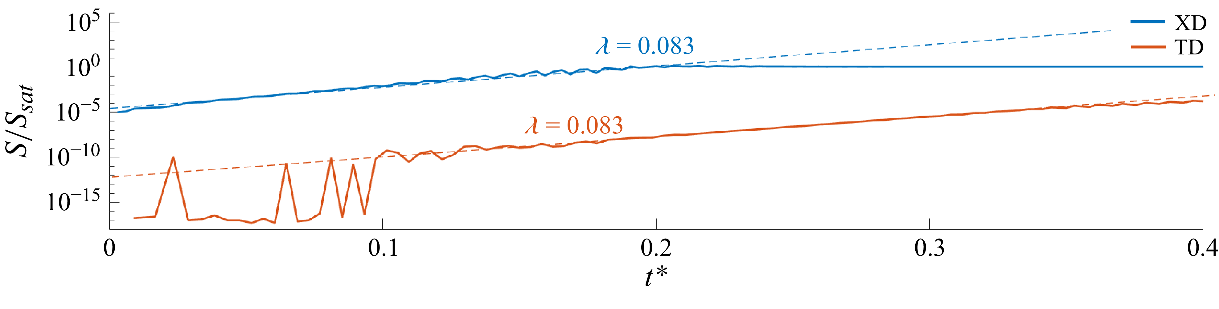
According to this parameter, the flame is symmetric with respect to the plane $y=W/2$ when $S=0$ . Non-zero values of $S$ indicate non-symmetric flames. To model its temporal evolution, we define (Rodríguez-Gutiérrez et al. Reference Rodríguez-Gutiérrez, Gómez-Miguel, Fernández-Tarrazo and Sánchez-Sanz2023) $ S = \mathcal{A} \exp (\lambda t/t_\delta ),$ with $t_\delta =\delta _T/s_{\textit{L}}$ the characteristic flame time and $\mathcal{A}$ the pre-exponential parameter that contains information of the size of the acoustic perturbation corresponding to the early stages of the process introduced into the system during ignition. The non-dimensional growth rate $\lambda$ , an eigenvalue of the problem that characterises the temporal evolution of the perturbation, remains invariant $\lambda =0.083$ for the two cases explored in our calculations as long as the flame remains symmetric, as can be seen in figure 4. Following the transition from a symmetric to a non-symmetric slanted flame at $t^* \simeq 0.2$ , $S$ saturates at $S_{\textit{sat}} \simeq 1.554 \times 10^{-4}$ as the growth rate diminishes, indicating stable flame propagation thereafter.

Figure 4.

Temporal evolution of the symmetry factor $S$ , scaled with the symmetry factor of the equilibrium non-symmetric slanted flame for the specified channel dimensions: $S_{\textit{sat}}=1.554\times 10^{-4}$ , at $t^*\simeq 0.2$ in the TD case. The figure shows the invariance of the eigenvalue with the boundary condition.

Figure 5.

Temporal evolution of the computed dominant frequency for XD (blue curve) and TD (orange curve) compared with the theoretical channel eigenmode frequency (black curve) (Clavin et al. Reference Clavin, Pelcé and He1990).

The difference in the magnitudes of the early-stage perturbation is related to the value of the pre-exponential factor $\mathcal{A}$ . As can be seen in figure 4, in the TD case, after interaction with the boundary condition at the exit, $S$ remains seven orders of magnitude smaller than in the XD case. It is clear that this initial disturbance produced by ignition (much smaller in the TD case) modifies the behaviour of the flame until it is extinguished. This explains why the flame requires much longer times to transition to a non-symmetric state, provided that the symmetric to non-symmetric transition is highly nonlinear the flame structure appears to be symmetric until the very last stage of the process when the symmetry factor $S$ is almost saturated.

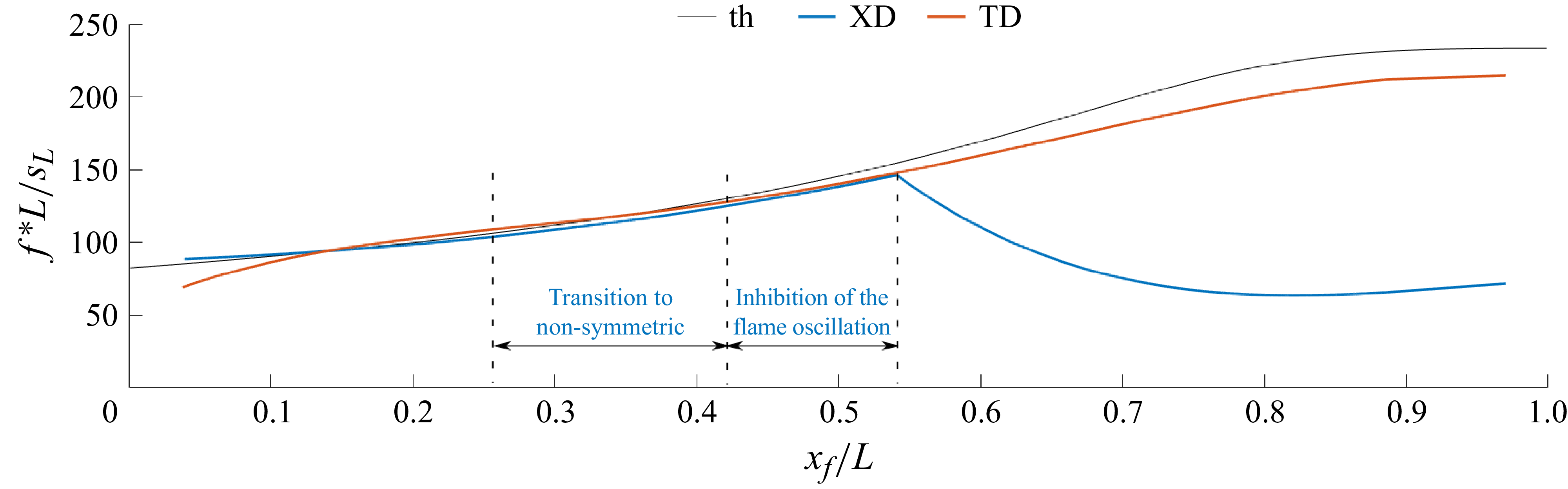
To better understand the physical origin of the observed oscillations, figure 5 shows the frequency of the fundamental mode $f^*$ as a function of the flame position within the channel $x_{\textit{f}}$ for both the XD and TD domains. The frequency is obtained by selecting the maximum from a sequence of power spectral decompositions of the pressure signal at the closed end of the channel ( $\Delta p/p_{\textit{a}}$ ) at different stages of flame propagation. These results are compared with the theoretical fundamental eigenmode frequency of the channel, derived for the asymptotic case of an infinitely thin planar flame advancing in an infinitely long slender adiabatic channel (Clavin et al. Reference Clavin, Pelcé and He1990).

A close agreement is observed between the theoretical prediction and the TD simulations, with differences below $8\,\%$ when the flame is located near the closed end of the channel. The small discrepancy is consistent with the simplifying assumptions in the asymptotic model – namely, an infinitely thin flame with respect to the acoustic wavelength, inviscid flow outside the flame zone and a one-dimensional channel and negligible flame propagation speed – which are only approximations of the physical configuration. Nonetheless, a similar fundamental mode frequency to Clavin et al. (Reference Clavin, Pelcé and He1990) is obtained by Pelcé & Rochwerger (Reference Pelcé and Rochwerger1992) and Dubey et al. (Reference Dubey, Koyama, Hashimoto and Fujita2019) for wrinkled flames. In the latter work (Dubey et al. Reference Dubey, Koyama, Hashimoto and Fujita2019), the effect of the flame propagation speed is quantified, observing a decrease of the eigenfrequencies for $x_{\textit{f}}/L\gt 0.5$ with increasing $s_{\textit{f}}$ . This effect contributes to the justification of the difference between the theoretical and numerical results as the effects of flame propagation speed are not considered in Clavin et al. (Reference Clavin, Pelcé and He1990). In the XD case, the oscillation frequency also follows the theoretical prediction up to $x/L \simeq 0.55$ . Beyond this point, however, the oscillations are progressively damped as the reactive front undergoes a transition to a non-symmetric flame shape. This loss of symmetry alters the coupling between the flame front and the acoustic field, thereby weakening the feedback mechanism responsible for sustaining oscillations.

Taken together, these results indicate that the dominant disturbances in the system arise from flame–acoustic interactions. The agreement with the channel eigenmode frequency confirms that the oscillations are essentially acoustic in nature, while the damping observed in the asymmetric regime highlights the critical role of flame symmetry in maintaining resonance and sustaining large-amplitude fluctuations.

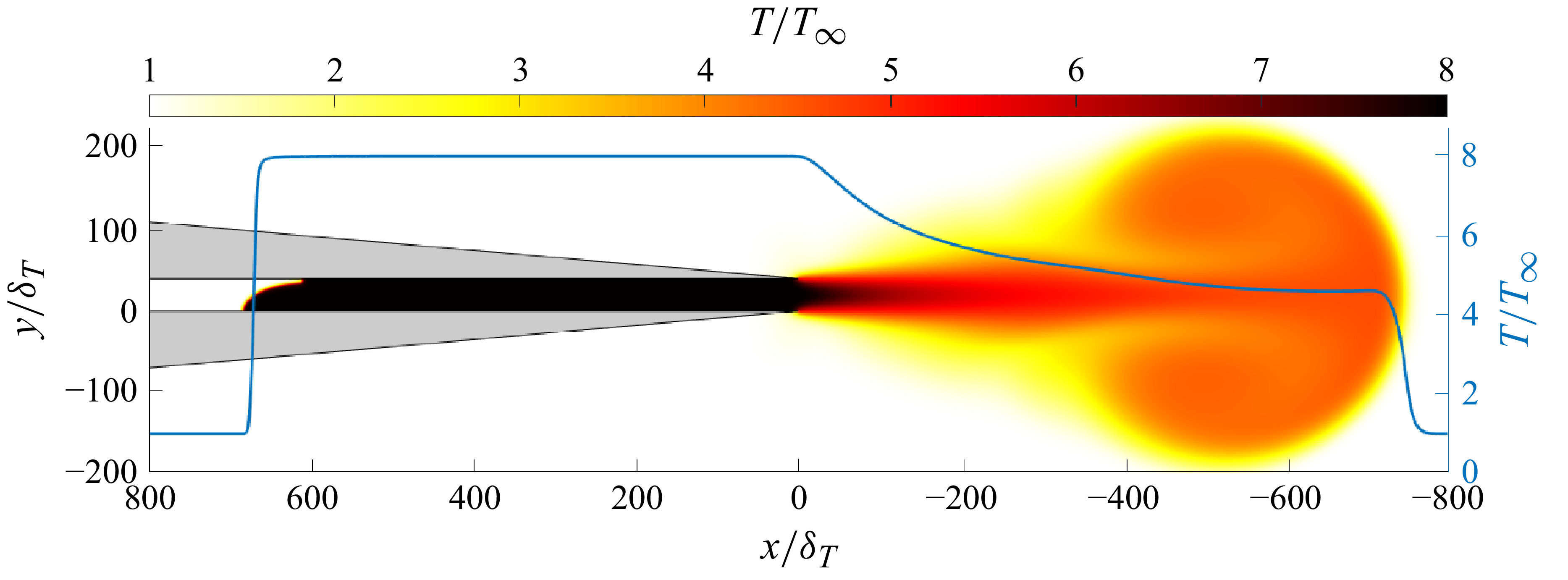
The use of the XD enables the description of the emerging hot jet formed after ignition, as can be seen in figure 6, composed basically of hot combustion products mixed with cold air. The jet emerges into the surrounding atmosphere lead by a hot counter-rotating vortex pair that remains hot until it reaches long distances from the channel’s exit. Figure 6 presents a snapshot of the temperature field and illustrates how the gas temperature remains equal to the adiabatic flame temperature within the channel, corresponding to the adiabatic boundary conditions imposed at the channel walls. Downstream of the exit ( $x \lt 0$ ), the jet cools as cold ambient air is entrained into the jet.

Figure 6.

Temperature field at dimensionless time $t^* = 0.3719$ for the XD configuration in a channel of length $L/\delta _T = 800$ and width $W/\delta _T = 40$ . The figure presents the temperature colour map together with the corresponding temperature profile along the channel centreline (blue line). See video in the supplementary material for temporal evolution.

Figure 6 also includes the longitudinal temperature profile along the symmetry plane, demonstrating that cooling occurs longitudinally as well, influencing the flame dynamics, especially during sub-atmospheric pressure phases that promote ambient air ingestion. Such downstream effects, not included in the TD case, also modify the velocity and mass-flow rate at the channel exit, $x=0$ . Their profiles are plotted in figure 7 for both XD figure 7(a) and TD domains figure 7(b) during the formation of the steady flame after ignition, different times of an oscillation cycle in the high-amplitude oscillatory mode and during the stationary flame propagation achieved once the oscillations have been damped.

We now examine the oscillation cycle of the high-amplitude mode. In the XD case, velocity and mass fraction oscillate with a phase shift relative to the pressure signal (Rodríguez-Gutiérrez et al. Reference Rodríguez-Gutiérrez, Gómez-Miguel, Fernández-Tarrazo and Sánchez-Sanz2025), leading to the entrainment of cold gas ( $\rho u \lt 0$ ) into the channel via the lateral boundary layers near the walls during low-pressure phases (figure 3). The temperature profile exhibits a transition from high values along the channel centreline to ambient conditions within the mixing layers of the discharge jet. This effect is absent in the TD case, where the burned gas retains a uniform temperature $T = T_{\textit{f}}$ at the channel exit $x = 0$ , as can be seen in the bottom panel of figure 7.

The velocity profiles, on the other hand, remain qualitatively similar in both cases. However, it is important to note that the XD case allows fluid entrainment into the channel at $t^*= 0.1797$ . This flow reversal also happens when pressure at the channel exit decreases below ambient pressure. These observations demonstrate that the thermochemical properties of the incoming fluid cannot, in general, be anticipated when the computational domain is truncated.

Figure 7.

Flow conditions at the channel exit at the times indicated in figure 3 (maximum-amplitude oscillation mode) for the XD (a) and TD (b) cases.

5.2. The acoustic energy contained in the channel

We start the analysis by considering the evolution of the acoustic energy, $E_{\textit{ac}}$ , defined in (3.1). The total acoustic energy stored in the channel is calculated as

(5.2) \begin{equation} \mathcal{E}_{\textit{ac}}(t) =\int _0^{L} \int _0^{W} E_{\textit{ac}}(x,y,t) \, dx \, dy. \end{equation}

Figure 8 shows the temporal evolution of $\mathcal{E}_{\textit{ac}}$ for the XD (blue line) and TD (orange line) cases, considering both the reactive (solid line) and inert (dashed line) configurations. The inert case represents the evolution of acoustic energy in a non-reactive mixture after an initial acoustic perturbation, introduced as a Gaussian hotspot centred at $x = 10\delta _T$ , identical to that of the reactive case, to illustrate the channel’s intrinsic dissipation rate.

The decay of acoustic energy is determined by both the channel geometry and the fluid properties. As shown in the figure, $\mathcal{E}_{\textit{ac}}$ decreases more rapidly in the XD case than in the TD case at early times. In the XD configuration, an exhaust jet forms at the channel exit to adjust local pressure gradients, thereby expelling acoustic energy in the process. This trend reverses for $t^* \gt 0.17$ , when the acoustic levels in the XD case exceed those in the TD case. Since no chemical sources are present in the inert configuration, this behaviour likely reflects the combined effects of external acoustic forcing in the XD case and artificial energy dissipation introduced by domain truncation in the TD case at $x = 0$ .

Figure 8.

Comparison of the acoustic energy $\mathcal{E}$ for the XD (blue line) and TD (orange line) configuration considering a reactive (continuous line) and non-reactive (dotted line) flow as a function of time.

For reactive flows (solid lines in figure 8), the magnitude of the initial acoustic energy introduced during the ignition process is the same as in the inert case. Chemical reactions sustain now the temperature gradients, which elevate the acoustic energy levels two orders of magnitude relative to the inert case. Subsequently, the acoustic energy decreases at a rate comparable to the inert case until high-amplitude instabilities develop. These instabilities develop earlier in the XD case, from $t^* \simeq 0.12$ , raising the acoustic energy levels as a consequence of the violent flame oscillations. The flame-front transition towards non-symmetric damps the instabilities and lowers the magnitude of the acoustic energy.

In the TD case, instabilities are triggered at $t^* \simeq 0.24$ , with the acoustic energy rising to a maximum before decreasing as the flame approaches the closed end of the channel and the instabilities vanish. Notably, the flame front remains symmetric throughout this process. In both cases, the acoustic energy drops sharply once the high-amplitude instabilities dissipate, approaching the trend observed in the inert configuration. The TD case exhibits a smooth decay of acoustic energy, whereas the XD case shows a noisier evolution due to fluctuations induced in the exhaust jet by preceding flame oscillations. This dynamics can be clearly observed in the video included in the supplementary material.

5.3. The sources of acoustic energy

To understand the time evolution of the acoustic energy, we analyse the individual terms in the transport (3.2). According to this equation, variations in $\mathcal{E}_{\textit{ac}}$ arise from changes in the source terms or from energy fluxes through the channel exit at $x = 0$ . In this section, we examine these acoustic energy sources to assess the relative contributions of the thermoacoustic source, arising from the interaction between pressure waves and the flame, and the aeroacoustic sources, associated with the vorticity field and the effects of the downstream mixing layer. Notice that, even though previous studies (Ducruix et al. Reference Ducruix, Schuller, Durox and Candel2003; Poinsot & Veynante Reference Poinsot and Veynante2005; Laera et al. Reference Laera, Campa, Camporeale, Bertolotto, Rizzo, Bonzani, Ferrante and Saponaro2014) typically considered only the thermoacoustic source term $D_{TA}$ , neglecting the aeroacoustic contribution, we retained $D_{AA}$ in our simulations to offer a critical evaluation of the effects of both energy sources in the overall acoustic energy balance. Figures in this section are complemented with videos in the supplementary material for a better comprehension of the processes explained.

Figure 9.

Temporal evolution of the aeroacoustic (AA, yellow line) and thermoacoustic (TA, red line) sources for the XD case. The upper and lower labels indicate the different flame propagation regimes and the evolution of the pressure oscillations amplitude, respectively. The insets highlight selected time instants within the oscillation cycle: (2)–(5) correspond to the phase of maximum high-amplitude instability (both sources in phase), and (6)–(8) to the transition toward a non-symmetric flame front (sources in counter-phase). These markers correspond to the violet and green shaded regions in figure 12, further analysed in figures 14 and 15.

We start the analysis by plotting in figure 9 the temporal evolution of the aeroacoustic $\mathcal{D}_{AA}$ and thermoacoustic $\mathcal{D}_{TA}$ sources integrated across the channel volume for the XD case, defined as

(5.3) \begin{equation} \mathcal{D}_{i} = \int _0^{W} \int _0^{L} D_{i} \,\text{d}x \,\text{d}y, \end{equation}

where i refers to the aeroacoustic or thermoacoustic acoustic source. To facilitate the reading, this figure uses a ‘potential’ scale for the y-axis as $(\mathcal{Y}/\mathcal{|Y|})\boldsymbol{\cdot }\mathcal{Y}^{1/10}$ , where $\mathcal{Y}$ represents a linear y-axis scale. This adaptive scale preserves information about relative magnitudes in a manner similar to a logarithmic scale, while avoiding the singularity at zero. It allows both positive and negative values of the source terms, with negative (positive) values of $\mathcal{D}_{i}$ representing sinks (sources) of acoustic energy.

The evolution of the sources shown in figure 9 can be summarised in three stages: suppression, reinforcement and cancellation. In the first phase, immediately after ignition, the flame dynamics is dominated by negative (suppressing) aeroacoustic sources that facilitate a smooth non-oscillatory flame propagation. Thermoacoustic sources are positive but several orders of magnitude smaller than the negative aeroacoustic sources $|\mathcal{D}_{TA}|/|\mathcal{D}_{AA}| \ll 1$ , what explains the decay of acoustic energy contained in the channel, as discussed in § 5.2.

In the second stage, that starts approximately at $t^* \sim 0.05$ , the aeroacoustic source becomes positive while the thermoacoustic source grows to become of the same order of magnitude as the aeroacoustic term, feeding them both the onset of the flame oscillations. The acoustic energy peaks at $t^* \sim 0.17$ , with the value of both $\mathcal{D}_{TA}$ and $\mathcal{D}_{AA}$ positive and in phase, thereby reinforcing the growth of acoustic energy, as shown in the black-box inset (in linear scale) of figure 9.

The flame oscillation continues until the flame transition to a non-symmetrical shape and flame propagation becomes, again, non-oscillatory. This occurs because the thermoacoustic $\mathcal{D}_{TA}$ and aeroacoustic $\mathcal{D}_{AA}$ sources are in counterphase, partially cancelling each other. This can be seen in the blue-box inset of the same figure (in linear scale). This agrees with previous observations that the non-symmetric slanted flame becomes free of oscillations (Jiménez et al. Reference Jiménez, Fernández-Galisteo and Kurdyumov2021; Rodríguez-Gutiérrez et al. Reference Rodríguez-Gutiérrez, Gómez-Miguel, Fernández-Tarrazo and Sánchez-Sanz2023). To the best of the authors’ knowledge, the present results provide the first quantitative explanation of the oscillation-damping mechanism associated with the transition to non-symmetric flames.

Figure 10.

Temporal evolution of the aeroacoustic (AA, yellow line) and thermoacoustic (TA, red line) sources for the TD case. The upper and lower labels indicate the different flame propagation regimes and the evolution of the pressure oscillation amplitude, respectively. The inset highlights selected time instants within the oscillation cycle corresponding to the phase of maximum high-amplitude instability, where both sources are in phase, $(2'){-}(4')$ . These markers correspond to the blue shaded region in figure 12, further analysed in figure 16.

The corresponding results for the TD case are included in figure 10. At first, the evolution looks similar to the XD case, but the behaviour soon diverges: after ignition $\mathcal{D}_{AA}$ quickly fades away, while $\mathcal{D}_{TA}$ levels off. High-amplitude oscillations are eventually set off by the thermoacoustic and aeroacoustic sources after $t^*=0.25$ .

As mentioned earlier, the very first moments after ignition play a crucial role in determining how the flame evolves. To gain deeper insight into this stage, we now examine the aeroacoustic source term $\mathcal{D}_{AA}$ in both the XD and TD cases. Traditionally, research has emphasised the interaction between acoustic pressure fluctuations $p'$ and unsteady heat release $\dot {q}_{\textit{comb}}'$ as the primary mechanism of sound generation in low–Mach-number combustion. This process, known as thermoacoustic noise $\mathcal{D}_{\textit{TA}}$ , has long been regarded as the dominant source. As shown in figure 11, however, a more complex picture emerges. This figure compares $\mathcal{D}_{AA}$ for the two domains under consideration. The inset, presented on a linear scale, highlights the principal differences. In the initial stages of flame formation, $\mathcal{D}_{AA}$ exhibits positive values in the XD case, whereas in the TD case it becomes negative, thereby attenuating the acoustic disturbances. This sign reversal reflects the dissipative character of the boundary condition in the TD configuration.

Figure 11.

Comparison of the temporal evolution of sound generation due to vorticity in the XD and TD cases. The inset highlights an oscillation cycle during the early stages of the combustion process after ignition, $(1){-}(1')$ . This period corresponds to the brown shaded region in figure 12 and is further analysed in figure 13.

Figure 12.

Summary of the main events observed during the flame propagation process: ignition $(1){-}(1')$ , shaded in brown; maximum-amplitude oscillation cycle for the XD case $(2){-}(5)$ , shaded in violet; transition from a symmetric to a non-symmetric flame front for the XD case $(6){-}(8)$ , shaded in green; and maximum-amplitude oscillation cycle for the TD case $(2'){-}(4')$ , shaded in blue.

To contextualise these results, figure 12 identifies the location in the channel at which the events highlighted in the insets of figures 9, 10 and 11 take place. In the following, these events are examined in greater detail in figures 13, 14, 15 and 16 through an analysis of the spatial distribution of the acoustic source terms at the indicated times.

Figure 13.

Colour maps of sound generation due to vorticity ( $D_{\textit{AA}}$ ) for the XD (a) and TD (b) cases shortly after ignition ( $t^* = 0.3125 \times 10^{-3}$ ). The corresponding domain is shaded in brown in the schematic shown in figure 12. The black line denotes the flame front.

Figure 14.

Colour maps of thermoacoustic (a) and aeroacoustic (b) sources and sinks for the realistic XD case at selected time instants within the cycle of maximum-amplitude acoustic instability. Panels (2)–(5) correspond to $t^*= 0.1756,\,0.1776,\,0.1795$ and $0.1815$ , respectively. The corresponding domain is shaded in violet in the schematic shown in figure 12. The black curves depicts the flame front at each instant.

Figure 14 Long description

The image contains two sets of graphs labeled (a) and (b), each with five panels numbered 2 to 5. Each set of graphs shows color maps of thermoacoustic and aeroacoustic sources and sinks for a realistic XD case at selected time instants within the cycle of maximum-amplitude acoustic instability. The corresponding domain is shaded in violet in the schematic shown in figure 12. The black line depicts the flame front at each instant. Panel (a) shows thermoacoustic sources and sinks, while panel (b) shows aeroacoustic sources and sinks. Each panel is a line graph with the x-axis labeled x/delta_T and the y-axis labeled y/delta_T. The color maps range from -6000 to 6000 for both thermoacoustic and aeroacoustic sources and sinks. The graphs show the distribution and intensity of these sources and sinks at different time instants within the cycle of maximum-amplitude acoustic instability. The black line in each panel represents the flame front at the corresponding time instant.

We start with figure 13, which presents the two-dimensional distributions of $\mathcal{D}_{AA}$ at $t^* \sim 3 \times 10^{-4}$ when the flame kernel forms shortly after ignition. This figure corresponds with the shaded region labelled as (1) in figure 12. At this point, pressure fluctuations have already generated vorticity fields that will amplify, or attenuate, the acoustic energy. In this figure is evident that the acoustic field develops in a time scale that is much shorter than the characteristic time of flame propagation. Comparing the two panels of figure 13, we can see that aeroacoustic inhibition $\mathcal{D}_{AA} \lt 0$ remains confined within the incipient vortices that are formed along the channel walls and at the channel’s exit in the XD case. Around the flame, the aeroacoustic energy in a strongly positive $\mathcal{D}_{AA}\gt 0$ , resulting in a net positive contribution to the acoustic energy budget. Conversely, in the TD case, a large sink of acoustic energy $\mathcal{D}_{AA} \lt 0$ develops near the exit section, leading to a net negative contribution that delays the onset of flame oscillations.

The spatial distribution of acoustic sources during flame propagation along the channel is shown in figure 14. For the XD case, both the aeroacoustic ( $\mathcal{D}_{AA}$ ) and thermoacoustic ( $\mathcal{D}_{TA}$ ) source terms are presented at the times corresponding to the onset of maximum flame oscillations (shaded region labelled (2)–(5) in figure 12, and indicated by circular symbols in the black-box inset of figure 9).

Figure 15.

Colour maps of thermoacoustic (a) and aeroacoustic (b) sink/sources for XD case, at selected instants of time within the cycle of flame-front transition towards non-symmetric structure: (6)–(8) correspond to $t s_{L}/{L} = 0.2017,\,0.2023,\,0.2029$ , respectively. In this time interval, the domain shown in the figures is shown shadowed in green in the sketch of figure 12. The black line shows the flame shape at each instant of time.

The results indicate that thermoacoustic sources are confined to localised regions in the immediate vicinity of the reaction zone, where the heat release attains non-zero values. In contrast, aeroacoustic sources are significant not only near the flame front but also within the mixing layers formed between the jet emerging from the channel exit and the surrounding atmosphere. For the thermoacoustic sources (figure 14 a), positive contributions, associated with an increase in acoustic energy $E_{\textit{ac}}$ , consistently dominate over negative ones. The aeroacoustic sources, shown in the left panel (b), exhibit a more balanced spatial distribution of positive and negative contributions (figure 14 b, panels (2)–(5)), with periods of net acoustic energy suppression (panel (2)) rapidly followed by phases of intense generation (panel (3)). This alternating behaviour had already been anticipated from the trends observed in the black-box inset of figure 9.

As the system transitions toward a non-symmetric, slanted flame configuration, the source distributions undergo marked changes. Figure 15, corresponding to the blue-box inset in figure 9, illustrates this evolution. The thermoacoustic source remains predominantly positive, whereas the aeroacoustic source develops extended regions of negative contribution (in green), leading to a net suppression of acoustic energy. This suppression of acoustic energy eliminates the oscillations of the flame, explaining the observations illustrated in figure 9. Note that the channel exit region is omitted in figure 15, as acoustic energy production and suppression are negligible near $x=0$ once the jet at the channel exit ceases its oscillations.

To complete the analysis, we analyse the TD in figure 16. The first difference comes from the flame shape, that adopts a symmetric tulip configuration that reaches its maximum oscillation amplitude at $t^* \sim 0.3$ . The thermoacoustic source remains mostly positive and localised near the flame front while the aeroacoustic source extends into the flame vicinity but is negligible elsewhere. As in the XD configuration, the aeroacoustic source exhibits broad regions of negative contribution, suppressing acoustic energy due to perturbations in the velocity and vorticity fields over a region larger than the reaction zone. Importantly, the artificial truncation of the channel excludes contributions from the downstream mixing layer, where additional acoustic interactions are actually taking place. This exclusion introduces an artificial damping effect that alters the flame propagation dynamics, as demonstrated above.

Figure 16.

Colour maps of thermoacoustic (a) and aeroacoustic (b) sink/sources for TD case, at selected instants of time within the cycle of maximum-amplitude acoustic instability: (2’), (3’) and (4’) correspond to $ts_{L}/{L} = 0.3009,\,0.3016,\,0.3023$ , respectively. In this time interval, the domain shown in the figures is shown shadowed in blue in the sketch of figure 12. The black line shows the flame shape at each instant of time.

5.4. The acoustic fluxes through the exit section

As stated in (3.2), the total acoustic energy in the channel can also vary due to the changes in acoustic flux through the exit. This term is plotted in figure 17 for the XD and TD cases. The instantaneous flow of acoustic power is shown to take alternating positive and negative values of an amplitude that varies as the acoustic energy level (this can be observed by comparing figures 8 and 17) and has the same order of magnitude as the aeroacoustic and thermoacoustic sources ( $\left | P_{\textit{ac}}/\Delta p_{\textit{ac}} W s_{\textit{L}} \right |_{\textit{max}} \sim \left | D_{\textit{ac}}/\Delta p_{\textit{ac}} W s_{\textit{L}} \right |_{\textit{max}} \sim 10^3$ , as shown in figures 9, 10 and 17).

Focusing on the XD case (blue line), the signal exhibits a predominance of positive values in the early stages ( $t^* \lt 0.10$ ), indicating that the acoustic flux leaving the channel exceeds that entering it. This behaviour suggests that the exchange of acoustic energy with the surrounding atmosphere has a globally stabilising effect. Nonetheless, an incoming acoustic flux persists throughout the entire process, continuously interacting with the flame and contributing to its destabilisation. This effect is particularly pronounced in the early stages, when the flame is located near the channel exit.

In the TD case (orange line), the acoustic flux initially matches the magnitude observed in the XD case but is rapidly overdamped by the boundary conditions. After $t^* \sim 0.10$ , the flux remains essentially zero, except for the interval $0.25 \lt t^* \lt 0.40$ , which coincides with the onset of a high-amplitude acoustic oscillation in the TD flame. During this period, the acoustic power flux remains negative ( $p'v' \lt 0$ ), indicating pressure fluctuations in counterphase with the velocity field. This contrasts with the XD case, where the flux alternates between positive and negative values due to the more complex pressure–velocity interactions captured in the resolved outer flow. The boundary conditions in the TD domain further suppress the acoustic response, yielding amplitudes several orders of magnitude lower than those in the XD case during the high-amplitude instability phase ( $0.12 \lt t^* \lt 0.25$ ).

Figure 17.

Comparison of the instantaneous acoustic power fluxes, $P_{\textit{ac}}$ , through the channel exit for XD and TD cases.