1. Introduction
Marine propulsion is a significant source of noise (Renilson, Leaper & Boisseau Reference Renilson, Leaper and Boisseau2013). This results in two major drawbacks. In civilian transportation it contributes to the environmental impact of shipping, with detrimental effects on marine life (Merchant Reference Merchant2019; Vakili, Ölcer & Ballini Reference Vakili, Ölcer and Ballini2020; Chou et al. Reference Chou, Southall, Robards and Rosenbaum2021). In addition, the noise from propellers is a major issue in negatively affecting the stealth capabilities of military boats (surface ships or submarines). Unfortunately, an accurate characterisation of the acoustic signature of marine propellers is still problematic. Laboratory experiments face, for instance, the problem of reflections, hindering accurate measurements and generating significant scattering across experiments conducted at different facilities (Tani et al. Reference Tani2020). Computational fluid dynamics is a powerful tool, able to provide a significant contribution to the field and complement experiments. The typical approach relies on the acoustic analogy (Lighthill Reference Lighthill1952), assuming that the effect of the acoustic waves on the fluid dynamics is negligible (examples can be found in the works by Wang, Lele & Moin Reference Wang, Lele and Moin1996, Brentner & Farassat Reference Brentner and Farassat1998, Farassat & Brentner Reference Farassat and Brentner1998, Morris & Farassat Reference Morris and Farassat2002, Casalino Reference Casalino2003, Karabasov et al. Reference Karabasov, Afsar, Hynes, Dowling, McMullan, Pokora, Page and McGuirk2010, Najafi-Yazdi, Brès & Mongeau Reference Najafi-Yazdi, Brès and Mongeau2011, Yang & Wang Reference Yang and Wang2013 and Wang, Wang & Wang Reference Wang, Wang and Wang2021). This assumption allows computing the acoustic pressure with numerical simulations, by solving the Ffowcs-Williams and Hawkings (FWH) equation (Ffowcs-Williams & Hawkings Reference Ffowcs-Williams and Hawkings1969).
The use of numerical simulations for the acoustic characterisation of marine propellers requires high-fidelity approaches, characterised by levels of accuracy and computational efforts beyond the typical in both industry and academia (for a review, see the work by Wang, Freund & Lele Reference Wang, Freund and Lele2006). Recent theoretical studies (Ianniello & De Bernardis Reference Ianniello and De Bernardis2015; Ianniello Reference Ianniello2016) reinforced this point. They revealed the need to carefully resolve the wake of marine propellers to achieve an accurate estimate of their acoustic signature, in contrast to the established assumptions from the field of aero-acoustics. Their analysis pointed out that, while in aero-acoustics the contribution by the quadrupole, nonlinear sources can be usually neglected, except for transonic and supersonic flow regimes, this is not the case in hydroacoustics. In his conclusions, Ianniello (Reference Ianniello2016) recommended the use of high-fidelity, eddy-resolving computations of marine propellers, able to reproduce properly the phenomena of instability of the large structures they shed, which are expected to have a major impact on their acoustic signature. This is not the case of most methodologies typically adopted, also for the acoustic characterisation of propellers, including Reynolds-averaged Navier–Stokes (RANS) simulations, relying on turbulence modelling (Özden et al. Reference Özden, Gürkan, Özden, Canyurt and Korkut2016; Bagheri et al. Reference Bagheri, Seif, Mehdigholi and Yaakob2017; Wu et al. Reference Wu, Huang, Wang, Cao and Zhu2018; Naseer et al. Reference Naseer, Uddin, Mubashar, Sajid, Ali and Akhtar2020).
Ianniello (Reference Ianniello2016) found his theoretical analysis in close agreement with his earlier studies dealing with marine propellers (Ianniello, Muscari & Di Mascio Reference Ianniello, Muscari and Di Mascio2013, Reference Ianniello, Muscari and Di Mascio2014), based on RANS computations: moving away from the propeller, they verified a very quick decay of the noise associated with the monopole and dipole terms, making that from the quadrupole terms non-negligible. However, in the same works they acknowledged that RANS is inherently not well suited to reproduce the dynamics of the vortices populating the propeller wake and their instability, which were expected to become the major source of noise at a short distance from the propeller through the quadrupole terms of FWH. This conclusion was confirmed in later studies (Lidtke, Humphrey & Turnock Reference Lidtke, Humphrey and Turnock2016; Sezen & Kinaci Reference Sezen and Kinaci2019; Sezen et al. Reference Sezen, Cosgun, Yurtseven and Atlar2021b), urging the need for more accurate techniques, as detached-eddy simulation (DES) or large-eddy simulation (LES), in order to be able to capture properly the propeller wake, cavitation phenomena and their contribution to noise from marine propulsion. To verify the latter point, Cianferra, Ianniello & Armenio (Reference Cianferra, Ianniello and Armenio2019a) conducted LES on a canonical case, represented by a square cylinder of finite spanwise extent, immersed in a uniform flow. Their eddy-resolving approach was able to verify the importance of the nonlinear sources in defining the hydroacoustic signature. They adopted indeed a direct approach to distinguish the monopole, dipole and quadrupole terms of the FWH equation, enabling a comparison across the several sources of noise.
In the field of marine propellers, Keller, Kumar & Mahesh (Reference Keller, Kumar and Mahesh2018) recently utilised the results of accurate LES computations on a grid consisting of 181 million volumes to conduct a study on the DTMB 4381 model in open-water conditions, based on the acoustic analogy. However, they still based their analysis on the assumption that the monopole and dipole terms dominate the quadrupole terms everywhere, in disagreement with the recommendations by Ianniello (Reference Ianniello2016). Therefore, the latter were not computed. The acoustic analogy, coupled with wall-modelled implicit LES, was adopted also by Bensow & Liefvendahl (Reference Bensow and Liefvendahl2016) to simulate a five-bladed propeller in the standalone and hull–propeller configurations. They utilised grids consisting of about 5 million and 27 million volumes for the two cases, respectively. They adopted the porous formulation by Di Francescantonio (Reference Di Francescantonio1997), which allowed them to take into account the contribution associated with the nonlinear sources. It should be noted, however, that the use of the porous formulation prevented from decoupling the signature of the linear and nonlinear components of sound. This decoupling potentially enables the direct verification of the theoretical analysis presented by Ianniello & De Bernardis (Reference Ianniello and De Bernardis2015) and Ianniello (Reference Ianniello2016). In addition, the porous formulation is typically affected by the issue of the spurious sound due to the eddies crossing the permeable surface of integration, although the recent works by Zhou, Wang & Wang (Reference Zhou, Wang and Wang2021a) and Zhou et al. (Reference Zhou, Wang, Wang and He2021b, Reference Zhou, Zang, Wang and Wang2022) proposed a fix to this problem. The porous approach was recently pursued by Stark & Shi (Reference Stark and Shi2021) and Kimmerl, Mertes & Abdel-Maksoud (Reference Kimmerl, Mertes and Abdel-Maksoud2021). In particular, Stark & Shi (Reference Stark and Shi2021) analysed the acoustic signature of four-bladed ducted thrusters, using data from improved delayed detached-eddy simulation (IDDES), conducted on an unstructured hexahedral mesh consisting of about 13 million elements. Implicit LES on grids composed of  $O(10^7)$ volumes was utilised by Kimmerl et al. (Reference Kimmerl, Mertes and Abdel-Maksoud2021) to study the Newcastle propeller and the P1595 test case.
Based on the conclusions by Ianniello (Reference Ianniello2016), Cianferra, Petronio & Armenio (Reference Cianferra, Petronio and Armenio2019b) and Cianferra & Armenio (Reference Cianferra and Armenio2021) utilised the results of a wall-modelled LES computation on a grid consisting of 3 million volumes to perform the acoustic analysis of the SVA VP1304 propeller. In contrast with earlier studies, the direct approach to the computation of the different terms of the FWH equation was pursued. In this way they were able to confirm the results of the theoretical study by Ianniello (Reference Ianniello2016), finding that as one moves away from the propeller, the volume terms become dominant. However, the studies by Cianferra et al. (Reference Cianferra, Petronio and Armenio2019b) and Cianferra & Armenio (Reference Cianferra and Armenio2021) were still based on rather coarse simulations, unable to reproduce the instability mechanisms of the wake, which are expected to enhance the role of the quadrupole terms. In addition, the tractor configuration they considered prevented the generation of the hub vortex. Its role in the wake dynamics of marine propellers is important. Therefore, its contribution to the radiated sound is significant and cannot be neglected.
In the present study we adopted data generated by LES computations on a submarine propeller (Posa et al. Reference Posa, Broglia, Felli, Falchi and Balaras2019b), conducted on a much finer grid than in earlier studies on the hydroacoustics of marine propellers, consisting of 840 million points. Results were carefully validated by Posa et al. (Reference Posa, Broglia, Felli, Falchi and Balaras2019b) against particle imaging velocimetry (PIV) experiments in the wake by Felli & Falchi (Reference Felli and Falchi2018). In the following, we show that the acoustic signature associated with the quadrupole sources of sound becomes more significant than that of the monopole and dipole terms. The quadrupole source even increases, owing to the development of wake instabilities. In comparison with the simulations reported by Cianferra et al. (Reference Cianferra, Petronio and Armenio2019b), those by Posa et al. (Reference Posa, Broglia, Felli, Falchi and Balaras2019b) utilised a computational grid two orders of magnitude finer and included also the signature of the hub vortex, which is the largest coherent structure shed by propellers. This was found to be a significant source of noise, characterised by frequencies smaller than the tonal noise. The tonal noise is dominant only in the near field, due to the linear terms and to the nonlinear acoustic sources associated with the tip vortices, which experience a faster break-up, in comparison with the hub vortex.
This paper reports a summary of the methodologies utilised for the solution of the flow (§ 2.1) and the acoustic analysis (§ 2.2). The set-up considered for the Navier–Stokes simulations and the computation of the terms of FWH is discussed in § 3. Then, the wake topology (§ 4.1.1), the correlation of the flow structures with the acoustic signature of the propeller (§ 4.1.2) and the spectral characterisation of the propeller wake (§ 4.1.3) are presented. In particular, phase-averaged statistics of the flow were utilised to extract quantities relevant to the acoustic emission from the propeller wake and identify the most significant sources of noise. The results of the hydroacoustic analysis are reported in § 4.2, including a comparison with experiments (§ 4.2.1) and both streamwise (§ 4.2.2) and radial (§ 4.2.3) evolution of the acoustic signature. Final conclusions are presented in § 5.
2. Methodology
2.1. Hydrodynamic model
The data utilised for the hydroacoustic analysis reported in this study were generated by LES computations, based on the solution of the filtered Navier–Stokes equations for incompressible flows in non-dimensional form:
 $$\begin{gather} \frac{\partial \tilde{u}_i}{\partial x_i} = 0, \end{gather}$$
 $$\begin{gather}\frac{\partial \tilde{u}_i }{\partial t} + \frac{\partial \tilde{u}_i \tilde{u}_j}{\partial x_j } ={-} \frac{\partial \tilde{p}}{\partial x_i} - \frac{\partial \tau_{ij}}{\partial x_j} + \frac{1}{Re} \frac{\partial^2 \tilde{u}_i}{\partial x_j^2} + f_i, \end{gather}$$
where  $i$ and
 $j$ are indices spanning the three directions in space,
 $x_i$ is the coordinate in space in the direction
 $i$,
 $\tilde {u}_i$ and
 $\tilde {p}$ are the filtered velocity component in the direction
 $i$ and the pressure, respectively,
 $t$ is time,
 $\tau _{ij}$ is the
 $ij$ element of the subgrid stress (SGS) tensor,
 $Re$ is the Reynolds number and
 $f_i$ is a forcing term. The Reynolds number comes from scaling the momentum equation using a reference velocity,
 $\mathscr {U}$, a reference length,
 $\mathscr {L}$, and the density
 $\rho$ of the fluid. It is defined as
 $Re=\mathscr {UL}/\nu$, where
 $\nu$ is the molecular viscosity of the fluid. In this study
 $\mathscr {U}=U_\infty$ and
 $\mathscr {L}=D$, where
 $U_\infty$ and
 $D$ are the free-stream velocity and the diameter of the propeller, respectively.
The SGS tensor comes from filtering the nonlinear terms of the momentum equation:
 \begin{equation} \tau_{ij}=\widetilde{u_iu_j}-\tilde{u}_i\tilde{u}_j ={-} \nu_t \left(\frac{\partial \tilde{u}_i}{\partial x_j} + \frac{\partial \tilde{u}_j}{\partial x_i}\right), \end{equation}
where  $\nu _t$ is the eddy viscosity. This was computed in the present study using the wall-adaptive local eddy viscosity (WALE) model by Nicoud & Ducros (Reference Nicoud and Ducros1999), which properly reproduces the limiting behaviour of the eddy viscosity in the vicinity of walls without ad hoc corrections.
The forcing term  $f_i$ in (2.2) was utilised to represent the action of the body on the flow, exploiting an immersed-boundary (IB) methodology. This technique allows decoupling the topology of the Eulerian grid, where the Navier–Stokes equations are resolved, from the geometry of the body, which is represented by a suitable Lagrangian grid. This is ‘immersed’ within the Eulerian grid, whose points are tagged as body, fluid and interface, depending on their position, relative to the Lagrangian grid. The forcing term
 $f_i$ is utilised to enforce proper conditions at the solid and interface points, whereas it is equal to zero at the fluid points. At the solid points of the Eulerian grid the velocity boundary condition is equivalent to the local velocity of the body. At the interface points the velocity condition is defined from a linear reconstruction of the solution, based on the no-slip requirement on the surface of the body, defined by the Lagrangian grid, and the fluid points surrounding the interface points. Practically, the explicit computation of
 $f_i$ is not required, since velocity conditions at the solid and interface points are directly enforced during the time integration.
The Navier–Stokes equations were discretised on a regular, staggered cylindrical grid, using second-order, central finite differences. The equation was integrated in time using a fractional-step method (Van Kan Reference Van Kan1986). The discretisation in time of all convective, viscous and SGS terms of radial and axial derivatives was based on the explicit, three-step Runge–Kutta scheme, whereas the implicit Crank–Nicolson scheme allowed relaxing the stability requirements otherwise arising at the axis of the cylindrical grid from the terms of azimuthal derivatives. The solution of the hepta-diagonal Poisson problem stemming from the continuity requirement was achieved using trigonometric transformations across the azimuthal direction and an efficient direct solver (Rossi & Toivanen Reference Rossi and Toivanen1999) to invert the resulting series of penta-diagonal systems of equations. The overall solver was demonstrated globally second-order accurate in both space and time by Balaras (Reference Balaras2004) and Yang & Balaras (Reference Yang and Balaras2006). Applications in the field of marine propulsion were recently reported by Posa et al. (Reference Posa, Broglia, Felli, Falchi and Balaras2019b), Posa, Broglia & Balaras (Reference Posa, Broglia and Balaras2019a, Reference Posa, Broglia and Balaras2020a,Reference Posa, Broglia and Balarasb, Reference Posa, Broglia and Balaras2021, Reference Posa, Broglia and Balaras2022) and Posa & Broglia (Reference Posa and Broglia2021, Reference Posa and Broglia2022).
In the following discussion the streamwise coordinates are with respect to the propeller plane. In addition, all simulation results only represent the resolved quantities, so the notation  $\widetilde {{\cdot }}$ for the filter operator is dropped.
2.2. Acoustic model
In this work the hydroacoustic analysis is based on the acoustic analogy (Lighthill Reference Lighthill1952), which assumes that the acoustic signal, arising from the flow, propagates in a quiescent, uniform and unbounded medium and does not affect the flow. This approach allows reconstructing the acoustic field in post-processing from the solution of the flow, whose procedure is discussed below. This reconstruction is based on the integral solution of the differential form of the FWH equation:
 \begin{align} & \left (\frac{1}{c_0^2} \frac{\partial^2}{\partial t^2} - \frac{\partial^2}{\partial x_i \partial x_j}\right) H(\,f)\hat{p} \nonumber\\ &\quad =\frac{\partial \{[\rho_0 v_{n} + \rho' (u_{n} - v_{n}) ] \delta ( f )\}}{\partial t} \nonumber\\ &\qquad - \frac{\partial \{[p' \hat{n}_i +\rho u_i (u_{n} - v_{n}) ] \delta (\,f) \}}{\partial x_i} + \frac{\partial^2 [T_{ij} H ( f ) ]}{\partial x_i \partial x_j }, \end{align}
where  $c_0$ is the speed of sound,
 $H$ and
 $\delta$ are the Heaviside and Dirac delta functions, respectively,
 $\hat {p}$ is the acoustic pressure,
 $\rho _0$ is a reference density,
 $\rho '$ is the deviation of the density from
 $\rho _0$ and
 $p'$ is the deviation of the hydrodynamic pressure from the reference value
 $p_0$. The function
 $f(\boldsymbol {x},t)$ is defined in such a way to identify the surface
 $S$ as location of points in space,
 $\boldsymbol {x}$, where
 $f(\boldsymbol {x},t)=0$, with the additional requirements that
 $f(\boldsymbol {x},t)<0$ for the points
 $\boldsymbol {x}$ placed within the region of space bounded by
 $S$ and
 $f(\boldsymbol {x},t)>0$ for those points
 $\boldsymbol {x}$ located outside. The quantity
 $v_n$ is the velocity component of the surface
 $S$ in the outward normal direction, whereas
 $u_n$ is the velocity of the flow along the same direction. Here
 $T_{ij}$ is the Lighthill tensor,
 $T_{ij}=\rho u_i u_j +[ (\,p-p_0) - c_0^2 (\rho - \rho _0)]\delta _{ij} - \sigma _{ij}$, where
 $\delta _{ij}$ is the Kronecker delta, and where
 $\sigma _{ij}$ is the viscous stress tensor, which can be usually considered negligible. Therefore, in the case of incompressible flows the Lighthill tensor can be computed as
 $T_{ij}=\rho u_i u_j + (\,p-p_0) \delta _{ij}$.
The Heaviside and Dirac delta functions define the region of integration of the FWH integral solution. Here  $V$ is the volume outside the region of space bounded by
 $S$,
 $H(\,f)=1$ for
 $\boldsymbol {x}$ located within
 $V$, whereas
 $H(\,f)=0$ elsewhere,
 $\delta (\,f) \neq 0$ only for
 $\boldsymbol {x}$ on the surface
 $S$ and
 $\boldsymbol {\nabla } H(\,f)$ =
 $\boldsymbol {\nabla } f \delta (\,f) = \boldsymbol {\hat {n}} \delta (\,f)$, where
 $\boldsymbol {\hat {n}}$ is the outward unit vector normal to
 $S$.
In the direct formulation (2.4) is integrated taking  $S$ to be the surface of the propeller. The integration of (2.4) results in the following integral form of the FWH equation:
 \begin{align} & 4 {\rm \pi}\hat{p}(\boldsymbol{x},t) \nonumber\\ &\quad =\frac{\partial}{\partial t} \int_S \left[\frac{\rho_0 v_n}{r |1-M_r|}\right]_\mathscr{T} {\rm d} S + \frac{1}{c_0}\frac{\partial}{\partial t} \int_S \left[\frac{p' \hat{n}_i \hat{r}_i}{r |1-M_r|} \right ]_\mathscr{T} {\rm d} S \nonumber\\ &\quad + \int_S \left[\frac{p' \hat{n}_i \hat{r}_i}{r^2 |1-M_r|} \right ]_\mathscr{T} {\rm d} S + \frac{1}{c_0^2}\frac{\partial^2}{\partial t^2} \int_V \left[\frac{T_{rr}}{r |1-M_r|} \right ]_\mathscr{T} {\rm d} V \nonumber\\ &\quad +\frac{1}{c_0}\frac{\partial}{\partial t} \int_V \left[\frac{3T_{rr} -T_{ii}}{r^2 |1-M_r|} \right ]_\mathscr{T} {\rm d} V+ \int_V \left[\frac{3T_{rr} -T_{ii}}{r^3 |1-M_r|} \right ]_\mathscr{T} {\rm d} V, \end{align}
where the vector  $\boldsymbol {r}=\boldsymbol {x}-\boldsymbol {y}$ and
 $r$ is its magnitude;
 $\boldsymbol {x}$ identifies the position of the observer,
 $\boldsymbol {y}$ is the source location,
 $M_r$ is the Mach number in the direction of
 $\boldsymbol {r}$,
 $\hat {\boldsymbol {r}}$ is the unit vector associated with
 $\boldsymbol {r}$,
 $T_{rr}=T_{ij} \hat {r}_i \hat {r}_j$ and
 $T_{ii}$ is the trace of the Lighthill tensor. Here
 $V$ represents the volume of space surrounding
 $S$, which should be selected including all important sources of noise.
 $\mathscr {T}$ is the emission time, given by
 \begin{equation} \mathscr{T} = t - r/c_0 = t - |\boldsymbol{x}(t)-\boldsymbol{y}(\mathscr{T)}|/c_0. \end{equation}
Of course, the compressibility delay, represented in (2.6) by the ratio  $r/c_0$, complicates substantially the computation of the integrals in (2.5). However, we verified that in the present case it is small enough to be neglected, as also reported in the earlier studies by Ianniello et al. (Reference Ianniello, Muscari and Di Mascio2013) and Cianferra et al. (Reference Cianferra, Petronio and Armenio2019b), dealing with the hydroacoustic analysis of marine propellers. This assumption (
 $\mathscr {T} \approx t$) is therefore legitimate for marine propellers, due to their small velocities in comparison with the speed of sound in water, and is exploited in the acoustic analysis reported here.
The first term on the right-hand side of (2.5) comes from the displacement of fluid by the body and is called thickness or monopole term, the second and the third terms are tied to the pressure on the surface of the body and are called loading or dipole terms, whereas the remaining volume integrals are the quadrupole terms and depend on the nonlinear sources of noise populating the flow field. In the following discussion the linear monopole and dipole terms are compared with the nonlinear components, demonstrating how the latter experience a rise across the near wake, becoming quickly the leading terms as the structures shed by the propeller develop instability phenomena.
3. Computational set-up
The present study deals with the seven-bladed submarine propeller INSEAN E1658, working in open-water (isolated) conditions. It was carefully characterised in the experiments by Felli & Falchi (Reference Felli and Falchi2018). Then, LES-IB was adopted by Posa et al. (Reference Posa, Broglia, Felli, Falchi and Balaras2019b) to perform its numerical study. A very close agreement was found between experiments and computations on both global parameters of performance and wake features. The results of those simulations are utilised in this study to analyse the acoustic signature of the propeller. In the following some details about the adopted computational set-up are recalled.
The Reynolds number was defined assuming as length scale the chord of the propeller blades at  $70\,\%$ of its radius,
 $c_{70\,\%R}$, and as velocity scale the relative velocity of the flow at the same radial location:
 \begin{equation} Re_p=\frac{c_{70\,\%R} \sqrt{(2{\rm \pi} n0.70R)^2+V^2}}{\nu} \approx 360\,000, \end{equation}
where  $n$ is the frequency of the propeller rotation,
 $R$ is its radius and
 $V$ the advance velocity, in this case equal to the free-stream velocity,
 $U_\infty$.
The advance coefficient was defined as
 \begin{equation} J=\frac{V}{nD}=0.56. \end{equation}
These particular values of  $Re_p$ and
 $J$ were selected referring to the experimental study carried out by Felli & Falchi (Reference Felli and Falchi2018), that we utilised in our earlier work (Posa et al. Reference Posa, Broglia, Felli, Falchi and Balaras2019b) to validate the overall approach. A value of
 $Re_p=3.6 \times 10^5$ is typical for conducting open-water tests and characterising the performance of propellers within experimental facilities. The advance coefficient
 $J=0.56$ is chosen for a higher rotational speed than the design value for the INSEAN E1658 propeller (corresponding to
 $J \approx 0.90$), with the purpose of reproducing highly loaded conditions and generating strong hub and tip vortices.
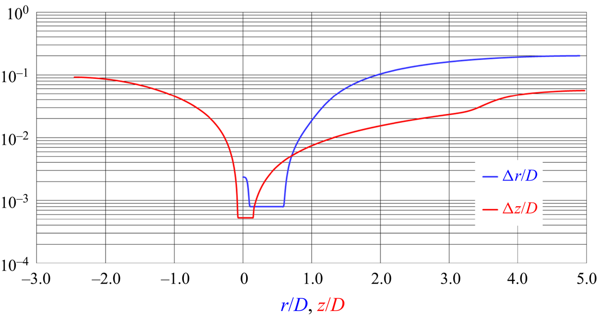
The simulation was conducted on an Eulerian, cylindrical grid consisting of  $800\times 1026\times 1026$ (840 million) points across the radial, azimuthal and axial directions, respectively. The angular spacing along the azimuthal direction was uniform, whereas stretching was adopted in the radial and axial directions to cluster points in the region of the propeller and its wake. It is also worth noting that the cylindrical topology of the grid inherently allowed increasing the resolution at smaller radii, in the area of interest. Figure 1 provides a visualisation of both radial and axial distributions of the grid spacing. The radial grid was uniform across the span of the propeller blades, with a spacing
 ${\rm \Delta} r/D=8.0 \times 10^{-4}$. The axial grid was uniform across the streamwise extent of the propeller blades, with a spacing
 ${\rm \Delta} z/D=5.3 \times 10^{-4}$. The azimuthal, linear spacing of the grid at
 $70\,\%$ of the radial extent of the propeller was equivalent to
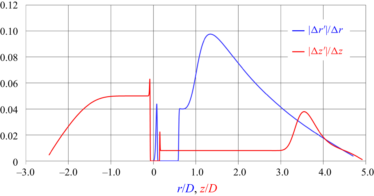
 $0.7R {\rm \Delta} \vartheta /D = 2.1 \times 10^{-3}$. For accuracy, care was taken to stretch the grid smoothly across both radial and axial directions. In particular, the ratio between the local derivative of the grid spacing and the grid spacing itself was kept well below
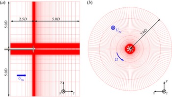
 $10\,\%$ across the whole extent of the computational domain, as shown in figure 2. More details on the resolution of the Eulerian grid can be found in the work by Posa et al. (Reference Posa, Broglia, Felli, Falchi and Balaras2019b), where validation and a detailed discussion of the flow features are reported. Two slices of the cylindrical grid are illustrated in figure 3, where for clarity of visualisation only 1 of every 64 points is shown.
Resolution of the cylindrical grid across the radial and axial directions.

Stretching of the cylindrical grid across the radial and axial directions.

Slices of the computational grid: simplified representation of 1 of every 64 points.

The Eulerian grid discretised a cylindrical domain extending from  $2.5D$ upstream of the propeller plane to
 $5.0D$ downstream of it. Its radial extent was equivalent to
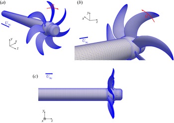
 $5.0D$. A uniform axial velocity was prescribed at the inlet boundary, whereas convective conditions on all three velocity components were utilised at the outlet boundary. Homogeneous Neumann conditions were prescribed at the lateral, cylindrical boundary of the domain. Homogeneous Neumann conditions were also utilised at all boundaries for pressure and eddy viscosity. In the framework of the IB methodology the geometry of the propeller was represented using a Lagrangian grid, consisting of 166 000 triangles. During the simulations, the rotation of this Lagrangian grid within the stationary, Eulerian grid was prescribed, based on the advance coefficient. The Lagrangian grid is represented in figure 4, enabling also the visualisation of the propeller geometry. In particular, it should be noted that, in agreement with the experiments conducted by Felli & Falchi (Reference Felli and Falchi2018), the propeller was simulated in the more realistic push configuration (shaft upstream of the propeller plane), allowing the generation of a large hub vortex.
Geometry of the INSEAN E1658 propeller, together with its Lagrangian grid.

The resolution in time was tied to that in space, as defined by the stability requirements of the adopted numerical scheme. Simulations were carried out at a constant value of the Courant–Friedrichs–Lewy (CFL) number, equal to 1. Therefore, the time step was computed as  ${\rm \Delta} t = ({\rm \Delta} x_i/u_i)_{max}$, where
 $i=1,2,3$ and
 $({\rm \Delta} x_i/u_i)_{max}$ is the maximum of the ratio between the local grid spacing along the direction
 $i$ and the local velocity of the flow in the direction
 $i$, evaluated across the whole extent of the computational domain. This resulted in a very fine time resolution, equivalent to a rotation of
 $0.06^{\circ }$ per time step. The solution of the flow was developed during one flow-through time, to remove the memory of initial transients. Then, statistics of the flow were computed at run time during 10 additional revolutions. Parallel computing was exploited, relying on calls to Message-Passing Interface (MPI) libraries, using 1024 cores of a distributed-memory cluster.
The hydroacoustic analysis of the propeller was conducted in post-processing, using instantaneous realisations of the flow from LES-IB. They included the whole extent of the computational domain, with the purpose of exploiting the direct approach to the computation of all volume terms of the integral FWH equation (2.5). More than four propeller rotations were considered, saving 168 solutions per revolution, for a total of 714 instantaneous realisations of the flow. The angular spacing between them was equal to  $2.14^{\circ }$, equivalent to a sampling frequency of
 $24 \,f_{bp}$, where
 $\,f_{bp}$ is the frequency of the blade passage. The surface terms of (2.5) were computed with the velocities of each element of the Lagrangian grid and the pressure values on them. They were interpolated at each instant in time from the solution of the flow on the Eulerian grid. The volume
 $V$ in (2.5) was taken to be a cylindrical subdomain of
 $z/D \in [-1.0, 4.5]$ and
 $r/D \leq 0.56$, with the purpose of including the whole radial extent of the wake shed by the propeller and its sound sources. Both
 $S$ and
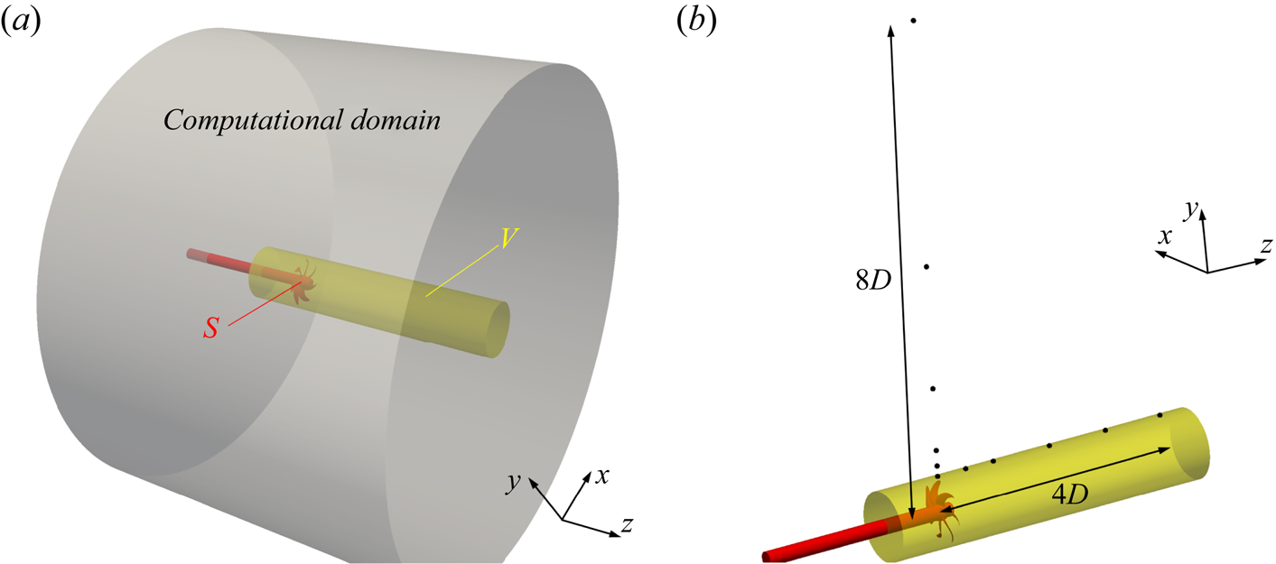
 $V$ are represented in figure 5(a), in red and yellow colours, respectively, within the computational domain of the LES simulations in grey. The hydrophones were distributed along both streamwise and radial directions, as shown in figure 5(b), in order to analyse the streamwise and radial evolution of the acoustic signature of the propeller.
(a) Surface,  $S$, and volume,
 $V$, of integration of the terms in (2.5), within the computational domain of the LES simulations; (b) positions of the hydrophones considered for the acoustic analysis of the propeller.

4. Results
4.1. Overview of the flow downstream of the propeller
In this section the main features of the propeller wake are presented. The fluid dynamics of this flow was already discussed in depth in our earlier work (Posa et al. Reference Posa, Broglia, Felli, Falchi and Balaras2019b). However, due to the complexity of the wake topology and its importance in defining the acoustic signature through the nonlinear component of sound, we decided to report in § 4.1.1 a summary of the main flow features. In addition, in § 4.1.2 we provide results for the Lamb vector, due to its correlation with the noise generated by vorticity and turbulence within the propeller wake. Eventually, § 4.1.3 provides the pressure and velocity spectra along the streamwise direction, to be correlated in § 4.2 with those of the acoustic pressure.
4.1.1. Wake topology
Phase-averaged statistics were computed on a cylindrical grid rotating with the propeller, with the purpose of isolating the coherent structures populating the wake, as long as they keep synchronised with the propeller rotation, before instability. The phase average of any quantity  $\mathcal {G}$ is defined as
 \begin{equation} \langle \mathcal{G} \rangle \left ( r, \vartheta, z \right) = \frac{1}{\mathcal{N}} \sum^{\mathcal{N}}_{i=1} \mathcal{G} \left ( r, \vartheta + \varOmega t_i, z, t_i\right), \end{equation}
where  $r$,
 $\vartheta$ and
 $z$ are the cylindrical coordinates on the Eulerian grid,
 $\varOmega = 2 {\rm \pi}n$ is the angular speed of the propeller,
 $\mathcal {N}$ is the size of the statistical sample and
 $t_i$ the time of the
 $i$th sample.
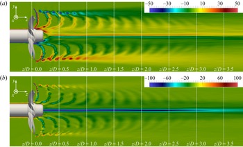
Figure 6 shows the azimuthal and axial components of the vorticity vector. Figure 6(a) highlights the signature of the tip vortices at outer radii in the near wake. This signature is quickly lost away from the propeller plane, because the tip vortices develop instability and lose their synchronisation with the rotation of the propeller blades, smearing out their footprint in the phase-averaged statistics of the wake. This occurs within the first diameter downstream. Figure 6(b) shows the presence of a strong hub vortex at the wake axis. The negative peak of axial vorticity there experiences a gradual diffusion moving downstream, due to the development of oscillations around the wake axis, but this process is slower than for the tip vortices, revealing that the hub vortex plays a longer-lasting role within the propeller wake, keeping coherent across wider distances downstream.
Contours of phase-averaged (a)  $x$ and (b)
 $z$ components of vorticity on a meridian plane through the propeller axis. Vorticity scaled by
 $U_\infty /D$.

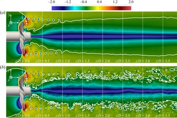
This point is also illustrated in figure 7, where both the phase average and an instantaneous realisation of the flow are visualised, considering both contours and isolines of the hydrodynamic pressure coefficient,  $c_p$. This was defined as
 $c_p=(\,p-p_\infty )/(0.5 \rho U_\infty ^2)$, where
 $p_\infty$ is the free-stream pressure, taken at the inlet of the computational domain. The isolines in figure 7 refer to a value of
 $c_p=-0.1$. They are useful to isolate the areas of low pressure, which are affected the most by the tip and hub vortices. In particular, it is shown that the influence by the hub vortex quickly spreads to outer radii, as also observed in the experimental studies reported by Felli, Camussi & Di Felice (Reference Felli, Camussi and Di Felice2011) and Felli & Falchi (Reference Felli and Falchi2018). The core of the hub vortex, although developing oscillations around the wake axis, remains distinct across the whole extent of the computational domain. In contrast, the tip vortices at the outer boundary of the wake experience break-up into smaller structures, feeding the process of turbulent energy cascade and contributing to the range of the highest frequencies of the sound coming from the propeller wake.
Contours of (a) phase-averaged and (b) instantaneous pressure coefficient on a meridian plane through the propeller axis. Isolines for a value of pressure coefficient  $c_p=-0.1$.

In figure 8 the results for the phase-averaged turbulent kinetic energy are reported, which is defined as  $k=1/2 [ (u_r')^2 + (u_\vartheta ')^2 + (u_z')^2 ]$, where
 $u_r'$,
 $u_\vartheta '$ and
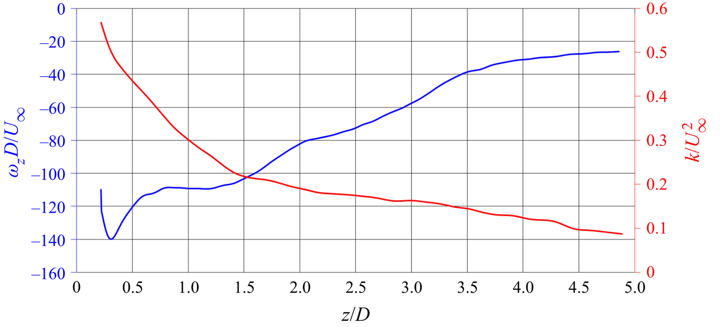
 $u_z'$ are the root-mean-squares of the radial, azimuthal and axial velocity components. Figure 8 displays the highest values of turbulent kinetic energy at the wake axis, due to the hub vortex. Those at the outer boundary of the wake, associated with the tip vortices, are also significant, but lower. In addition, as the wake develops instability the maxima in figure 8 experience diffusion, which is the result of growing fluctuations by both tip and hub vortices. In particular, the diffusion of the axial peaks of vorticity and turbulent kinetic energy is shown in figure 9, where their streamwise evolution is reported. Both of them display a gradual decay just downstream of the onset of the hub vortex.
Contours of phase-averaged turbulent kinetic energy on a meridian plane through the propeller axis. Values scaled by  $U_\infty ^2$.


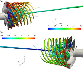
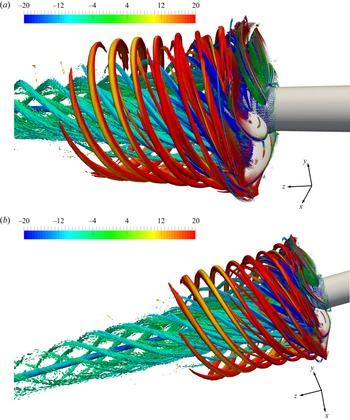
For the sake of clarity a three-dimensional visualisation of the wake structures is reported in figure 10, dealing with phase-averaged statistics. They show isosurfaces of the second invariant of the velocity gradient tensor (the Q-criterion by Hunt, Wray & Moin Reference Hunt, Wray and Moin1988), coloured by azimuthal and axial vorticity in the top and bottom panels, respectively. They demonstrate that the near wake is actually populated by a wealth of structures across all radii, in addition to the stronger hub and tip vortices. As for the tip vortices, they have a helical trajectory, whose pitch angle decreases from inner towards outer radii. They are also synchronised with the rotation of the propeller blades, so they contribute to the tonal component of the sound produced by its wake. They are smaller and less intense than the tip vortices, but they keep coherent further downstream, especially at the smallest radii, as shown in figure 11, where a lower value of  $Q$ was selected for the inner structures to be better distinguishable. In fact, the smaller pitch of the tip vortices, corresponding to a shorter relative distance between them, contributes to their stronger interaction. This accelerates their process of instability through mutual inductance phenomena, as discussed by Felli et al. (Reference Felli, Camussi and Di Felice2011), where the pitch of the tip vortices was modified by changing the rotational speed of the marine propeller INSEAN E779A. Both panels of figure 10 provide further evidence that the signature of the hub vortex remains distinct far downstream, in comparison with all other structures shed by the propeller. It should be noted that, although on average the core of the hub vortex keeps obviously oriented along the wake axis, this structure develops instantaneous fluctuations around it, as demonstrated by the pressure contours in figure 7(b). This is the reason why the values of axial vorticity at its core in figure 10(b) undergo a decrease.
Phase-averaged isosurfaces of  $QD^2/U_\infty ^2=100$, coloured by (a) azimuthal and (b) axial vorticity in the top and bottom panels, respectively. Vorticity scaled by
 $U_\infty /D$.

Phase-averaged isosurfaces of  $QD^2/U_\infty ^2=40$, coloured by azimuthal vorticity. Vorticity scaled by
 $U_\infty /D$.

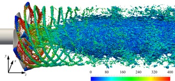
Figure 12 reinforces the last point. An instantaneous visualisation is illustrated, using isosurfaces of pressure coefficient, coloured by vorticity magnitude. As a result of the growing fluctuations of the hub vortex, the region of low pressure at the wake axis spreads towards outer radii, while the tip vortices lose their coherence and break up into smaller structures. As discussed later in § 4.2, these phenomena result in increasing levels of acoustic pressure within the near wake, involving both small and large frequencies: the former are due to phenomena of wake meandering, the latter to the instability and break-up of the large structures, starting the process of turbulent energy cascade.
Instantaneous isosurfaces of pressure coefficient ( $c_p=-0.4$), coloured by vorticity magnitude. Vorticity scaled by
 $U_\infty /D$.

4.1.2. Identification of the major sources of noise in the wake
In this section the major sources of noise populating the propeller wake are identified through the Lamb vector, which is the cross product of the vorticity and velocity vectors,  $\boldsymbol {L} = \boldsymbol {\omega } \times \boldsymbol {u}$, and appears as a source in the Powell acoustic analogy (Powell Reference Powell1964). For more details about Powell's vortex sound theory the reader is referred also to Felli, Falchi & Dubbioso (Reference Felli, Falchi and Dubbioso2015).
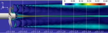
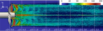
The root-mean-squares of  $|\boldsymbol {L}|$ are shown in figure 13, in terms of phase-averaged statistics. Just downstream of the propeller plane the highest values occur in the wake of each blade, in particular at the outer radii, populated by the tip vortices. Already at a half-diameter downstream the highest fluctuations occur at the wake axis, demonstrating the importance of the hub vortex in influencing the acoustic signature of the overall wake system. However, at the same streamwise location the values achieved at the outer radii are still significant. Moving further downstream the axial peak keeps stronger than the outer ones, which experience a faster diffusion, due to the faster instability of the tip vortices.
Contours of the phase-averaged root-mean-squares of the magnitude of the Lamb vector on a meridian plane through the wake axis.

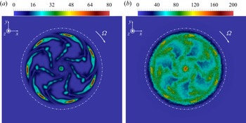
The wake of the propeller is illustrated in more details in figure 14 at the streamwise coordinate  $z/D=0.5$ by both first- and second-order phase-averaged statistics. Although the highest values of the Lamb vector are achieved at the core of the tip vortices, which are still quite coherent, the highest fluctuations in time affect the wake axis. Nonetheless, at
 $z/D=0.5$ the tip vortices as well as the shear layer shed from each propeller blade have still a significant role in terms of unsteadiness of the Lamb vector, especially because they affect a wider extent of the propeller wake, if compared with the hub vortex.
Contours of phase-averaged (a) first-order (mean) and (b) second-order (root-mean-squares) statistics of the magnitude of the Lamb vector on a cross-section placed at  $z/D=0.5$. The dotted-dashed line encompasses the projection of the area swept by the propeller blades.

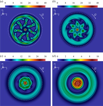
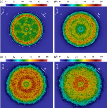
Further downstream the tip vortices lose their coherence, due to instability, whereas the hub vortex keeps the leading wake structure, as demonstrated by the phase-averaged contours in figure 15: the local maxima at the wake outer boundary are replaced by a diffused area of lower values of  $|\boldsymbol {L}|$, whereas the highest values are achieved at inner radii, associated with the large hub vortex. This is also the case for the second-order statistics, as shown in figure 16, where the root-mean-squares in time are visualised. Figure 16(a) shows that in the near wake at
 $z/D=1.0$ the tip vortices are able to affect a wide area at the outer boundary of the propeller wake, thus resulting in their leading influence on the acoustic signature. This is also the case in figure 16(b), where the streamwise coordinate
 $z/D=2.0$ is considered. However, further downstream the area of the largest time fluctuations moves to inner radii, suggesting a switch from an acoustic signature dominated by the tip vortices and the structures generated by their instability to an acoustic signature affected especially by the phenomena of instability occurring at the wake core, involving the hub vortex.
Contours of phase-averaged magnitude of the Lamb vector on cross-sections placed at (a)  $z/D=1.0$, (b)
 $z/D=2.0$, (c)
 $z/D=3.0$ and (d)
 $z/D=4.0$. The dotted-dashed line encompasses the projection of the area swept by the propeller blades.

Contours of phase-averaged root-mean-squares of the magnitude of the Lamb vector on cross-sections placed at (a)  $z/D=1.0$, (b)
 $z/D=2.0$, (c)
 $z/D=3.0$ and (d)
 $z/D=4.0$. The dotted-dashed line encompasses the projection of the area swept by the propeller blades.

4.1.3. Spectral analysis of the wake
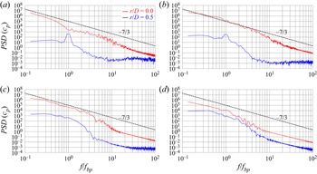
Figure 17 shows results for the power spectral density (PSD) of the hydrodynamic pressure coefficient in the wake of the propeller. The four panels refer to streamwise positions at  $z/D=0.25$,
 $z/D=0.50$,
 $z/D=1.0$ and
 $z/D=2.0$. Comparisons between the radial locations
 $r/D=0.0$ and
 $r/D=0.5$ are considered. The results in figure 17 demonstrate that a wide range of frequencies was resolved, reproducing for the inertial ones the
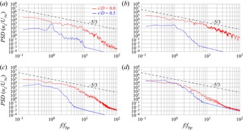
 $-$7/3 slope expected from Kolmogorov's theory. Interestingly, pressure fluctuations are substantially higher at the wake axis than at its outer boundary, providing additional evidence of the importance of the hub vortex in the wake dynamics. High levels of pressure fluctuations gradually extend to outer radii across the downstream development of the propeller wake. Similar results are shown in figure 18, dealing with the PSD at the same locations, but for the time history of the streamwise velocity at the selected probes within the propeller wake. As expected, in this case the slope in the range of the inertial frequencies approximates the value
 $-$5/3, especially in the wake core. It should be noted that pressure and velocity fluctuations at
 $r/D = 0.5$ are already growing between
 $z/D=0.25$ and
 $z/D=0.5$, where the influence by the hub vortex is still limited and the tip vortices remain coherent. This is consistent with the dynamics of the tip vortices. Their instability is a gradual process, resulting in growing levels of pressure and velocity fluctuations through phenomena of long-wave and short-wave oscillations of their trajectories, leading eventually to mutual inductance. This instability is reinforced as the wake develops downstream, also as a result of the interaction with the hub vortex (see for more details Posa et al. Reference Posa, Broglia, Felli, Falchi and Balaras2019b, Reference Posa, Broglia and Balaras2022).
Power spectral density of the hydrodynamic pressure coefficient at probes placed at the streamwise coordinates (a)  $z/D=0.25$, (b)
 $z/D=0.50$, (c)
 $z/D=1.0$ and (d)
 $z/D=2.0$: comparison between radial locations at
 $r/D=0.0$ and
 $r/D=0.5$. The dashed line is for the slope in the inertial range of frequencies for pressure from Kolmogorov's theory on homogeneous, isotropic turbulence.

Power spectral density of the streamwise velocity at probes placed at the streamwise coordinates (a)  $z/D=0.25$, (b)
 $z/D=0.50$, (c)
 $z/D=1.0$ and (d)
 $z/D=2.0$: comparison between radial locations at
 $r/D=0.0$ and
 $r/D=0.5$. The dotted-dashed line is for the slope in the inertial range of frequencies for velocity from Kolmogorov's theory on homogeneous, isotropic turbulence.

4.2. Analysis of the acoustic signature of the propeller
4.2.1. Comparisons with the experiments
The numerical hydrodynamic results utilised for the present hydroacoustic analysis were extensively validated in the earlier work by Posa et al. (Reference Posa, Broglia, Felli, Falchi and Balaras2019b). Both the parameters of global performance and the flow fields in the wake were found in excellent agreement with the dynamometric and PIV measurements conducted by Felli & Falchi (Reference Felli and Falchi2018). In this section, comparisons will be also provided dealing with the sound pressure level (SPL) generated by the propeller. We define SPL as
 \begin{equation} \textrm{SPL} = 20 \log_{10} \left(\frac{\hat{p}}{\hat{p}_0}\right), \end{equation}
where the reference acoustic pressure  $\hat {p}_0$ was taken equal to
 $1\,\mathrm {\mu }$Pa, as is typical for underwater noise.
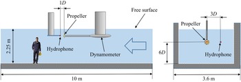
The experiment was performed in the Large Cavitation Channel at CNR-INM. Details on the facility are available in the works by Felli, Falchi & Pereira (Reference Felli, Falchi and Pereira2010) and Di Mascio et al. (Reference Di Mascio, Dubbioso, Muscari and Felli2015). The propeller, having a diameter of  $D=0.25$ m, was mounted backwards in the typical push-type arrangement, as shown in figure 19. Although this configuration yields non-homogeneous inflow conditions, due to the wake from the nacelle and the strut, it was preferred over the pull-type arrangement (i.e. propeller mounted forward, in front of the shaft), because in the latter case the shaft would interfere with the propeller wake, affecting its dynamics significantly (Cianferra et al. Reference Cianferra, Petronio and Armenio2019b).
Experimental set-up of the hydrophone measurements in the Large Cavitation Channel at CNR-INM.

The set-up consisted of a hydrophone, placed  $0.5D$ downstream of the propeller plane at a radial distance of
 $1D$ from its axis (see figure 19). The hydrophone was a miniature, high-sensitivity transducer, suitable for performing absolute sound measurements over the frequency range between 0.1 and 180 kHz and with a receiving sensitivity of
 $-$211 dB or 1 V
 $\mathrm {\mu }$Pa
 $^{-1}$ (Brüel & Kjær 8103 model). Hydrophone signals were conditioned by the Brüel & Kjær ‘NEXUS’ charge amplifier and then acquired by a multi-channel 24-bit acquisition system (PROSIG P8200). The A/D converter was set up to sample pressure fluctuation signals at 100 kHz, equivalent to 800
 $\,f_{bp}$, during 90 s. Any unwanted contribution from turbulence and vortex flow on measured pressure fluctuation signals was filtered out using the technique discussed by Felli, Grizzi & Falchi (Reference Felli, Grizzi and Falchi2014). This returned acoustic pressure fluctuation signals decontaminated from any hydrodynamic perturbation. The problem of separating the acoustic (sound) and the hydrodynamic (pseudo-sound) pressure fluctuations was tackled through a filtering method, based on the wavelet transform (Farge, Schneider & Kevlahan Reference Farge, Schneider and Kevlahan1999). This method exploits the peculiar ability of the wavelet transform to identify intermittent events (Ruppert-Felsot, Farge & Petitjeans Reference Ruppert-Felsot, Farge and Petitjeans2009) as well as the different nature of the pressure fluctuations associated with the hydrodynamic and acoustic perturbations, which are intermittent and homogeneous, respectively. Their separation is achieved through the selection of a proper threshold. This allows dividing the wavelet coefficients into two sets, depending on their values relative to the threshold level. Then, they are anti-transformed from the wavelet to the physical space to obtain separated sound and pseudo-sound pressure fluctuation signals. A more extensive discussion dealing with the separation method, together with examples of practical implementations of the technique, are reported by Felli et al. (Reference Felli, Grizzi and Falchi2014, Reference Felli, Falchi and Dubbioso2015).
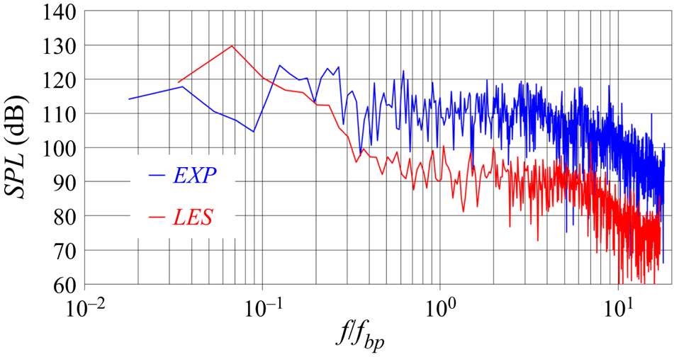
Figure 20 shows the results from both experiments and LES computations. The frequencies on the horizontal axis were scaled by the frequency of the blade passage,  $\,f_{bp}$. The agreement is satisfactory, especially taking into account the challenge of performing acoustic measurements in a confined environment, as well as the modelling assumptions of the simulations. In particular, the comparison in figure 20 shows that the experiment has higher SPL than the simulation. It is likely that the effects of reverberation from the walls of the experimental facility, free-surface (Cianferra & Armenio Reference Cianferra and Armenio2021), self-induced noise from the hydrophone and the background noise in the experiments, all missing in the computations, contribute to higher SPLs. In addition, both experiments and computations were carried out in absence of cavitation phenomena: in such conditions the propeller is quite silent, making even more demanding capturing accurately its acoustic signature. The issue of performing accurate acoustic measurements was extensively demonstrated by the ‘round Robin’ experimental study recently reported by Tani et al. (Reference Tani2020). They verified a significant scatter across measurements of the sound produced by a marine propeller, conducted in different facilities. In particular, the deviations across experiments were often above the values of 20 dB shown in figure 20. It should also be noted that comparisons between experiments and computations on the noise from marine propellers were rarely reported in the literature (for a few exceptions see Bensow & Liefvendahl Reference Bensow and Liefvendahl2016, Ebrahimi, Seif & Nouri-Borujerdi Reference Ebrahimi, Seif and Nouri-Borujerdi2019, Sezen et al. Reference Sezen, Atlar, Fitzsimmons, Sasaki, Tani, Yilmaz and Aktas2020, Sezen, Atlar & Fitzsimmons Reference Sezen, Atlar and Fitzsimmons2021a, Kimmerl et al. Reference Kimmerl, Mertes and Abdel-Maksoud2021 and Lidtke et al. Reference Lidtke, Lloyd, Lafeber and Bosschers2022, where also similar or more significant deviations were found). Therefore, the results in figure 20 compare well with similar studies in the literature and can serve as a useful reference to assess the performance of high-fidelity simulations in matching acoustic measurements.
SPLs at the radial coordinate  $r/D=1.0$ and the streamwise coordinate
 $z/D=0.5$: comparison between experiments and computations.

4.2.2. Streamwise evolution of the acoustic signature
Results for the streamwise evolution of the SPLs from the LES computations are reported in figure 21. Hydrophones located at the radial coordinate  $r/D=0.58$ are considered at five streamwise positions:
 $z/D=0.0$,
 $z/D=0.5$,
 $z/D=1.0$,
 $z/D=2.0$ and
 $z/D=3.0$. At
 $z/D=0.0$ the peaks at
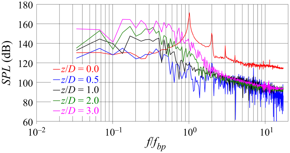
 $\,f_{bp}$ and its higher harmonics are well distinguishable and dominate the acoustic signature of the propeller. This is already not the case at
 $z/D=0.5$, characterised by a drop of the SPLs across all frequencies, with the exception of the lowest ones. Interestingly, moving further downstream the acoustic signature at the lowest frequencies experiences even an increase. As suggested by the hydrodynamic analysis of the flow, reported earlier by Posa et al. (Reference Posa, Broglia, Felli, Falchi and Balaras2019b), this behaviour can be attributed to the increasing instability of the wake system. In particular, the hub vortex, whose oscillations around the wake axis are characterised by frequencies lower than
 $\,f_{bp}$, extends quickly its footprint to outer coordinates, as discussed in § 4.1.1. However, it should be acknowledged that wake meandering is typically characterised by very small frequencies, which we were unable to investigate in detail, due to the required large period of integration in time and the prohibitive computational cost when using the present approach. Nonetheless, wake meandering phenomena affecting axial-flow rotors were already reported in the literature as a typical feature of their wake (Kang, Yang & Sotiropoulos Reference Kang, Yang and Sotiropoulos2014; Foti, Yang & Sotiropoulos Reference Foti, Yang and Sotiropoulos2018). The oscillations of the hub vortex, also discussed by Felli et al. (Reference Felli, Camussi and Di Felice2011), accelerate the process of instability of the tip vortices, whose break-up into smaller structures provides more energy also to higher frequencies, through the process of turbulent energy cascade, as shown in figure 21.
SPLs at hydrophones placed at the radial coordinate  $r/D=0.58$ across five streamwise locations, ranging from
 $z/D=0.0$ to
 $z/D=3.0$.

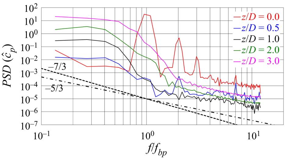
The strong correlation between the process of energy cascade of turbulence and the levels of acoustic pressure is demonstrated in more detail in figure 22, where results for the spectral analysis of the noise generated by the propeller are represented in terms of PSD of a pressure coefficient for the acoustic pressure,  $\hat {c}_p$, defined as
 \begin{equation} \hat{c}_p=\frac{\hat{p}-p_\infty}{0.5 \rho U_\infty^2}. \end{equation}
In figure 22 the slopes for velocity ( $-$5/3) and pressure (
 $-$7/3) fluctuations from Kolmogorov's theory on homogeneous, isotropic turbulence within the inertial range of frequencies are reported by dotted-dashed and dashed lines, respectively. It is important to clarify that in the results of figure 22 only the integral and the largest inertial scales are represented. The present simulation was actually able to resolve a much wider range of scales, as demonstrated in § 4.1.3, but data for the hydroacoustic analysis were saved with a period two orders of magnitude larger than the size of the step of advancement in time of the solution, due to storage requirements. Therefore, the analysis of the acoustic pressure was able to capture only the largest inertial scales. Nonetheless, the results in figure 22 are very interesting, because they demonstrate that at downstream locations the inertial range of frequencies of the acoustic pressure approaches the
 $-$5/3 behaviour of velocity, more than the
 $-$7/3 one of the hydrodynamic pressure, indicating that the acoustic signal at those frequencies is dominated by the fluctuations of velocity arising from the process of turbulent energy cascade, rather than by those of the hydrodynamic pressure. It should be noted that the smallest frequencies shown in figure 22 deviate from Kolmogorov's slope, because pressure fluctuations in that range are still dominated by the largest scales, especially those associated with the tip vortices and the wake shed by each blade, and turbulence is still far from Kolmogorov's hypotheses of homogeneity and isotropy. Nonetheless, when the turbulent cascade moves energy towards higher frequencies the behaviour of the spectra approaches the well-known
 $-$5/3 slope.
PSD of  $\hat {c}_p$ at hydrophones placed at the radial coordinate
 $r/D=0.58$ across five streamwise locations, ranging from
 $z/D=0.0$ to
 $z/D=3.0$. Dotted-dashed and dashed lines are the slopes in the inertial range of frequencies for velocity and hydrodynamic pressure, respectively, from Kolmogorov's theory on homogeneous, isotropic turbulence.

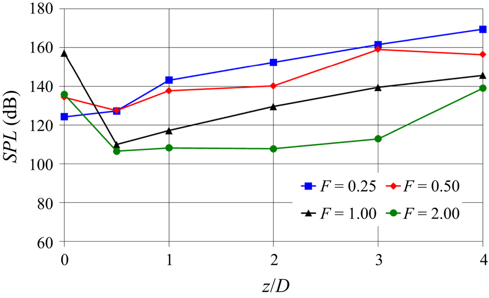
With the purpose of summarising the results in figure 21, SPLs were computed in one-third octave bands at some selected frequencies. They are reported in figure 23. There the four sets of data refer to frequencies  $f/f_{bp}=0.25$,
 $f/f_{bp}=0.50$,
 $f/f_{bp}=1.00$ and
 $f/f_{bp}=2.00$, respectively. Figure 23 highlights that the streamwise evolution at the lowest frequency is monotonically increasing, due to the growing large-scale instability of the wake system. For increasing frequencies the streamwise evolution becomes non-monotonic, with the inversion from the decreasing to the increasing trends moving downstream; as demonstrated by our analysis, dealing with the PSDs of the acoustic pressure, this may be a result of the process of turbulent energy cascade, operating a transfer of energy from the lowest to the highest frequencies. Although in the vicinity of the propeller SPLs are dominated by the frequency of the blade passage, moving downstream the lowest frequencies become the leading ones, achieving SPLs even higher than those produced over the propeller plane at
 $z/D=0.0$. This result is consistent with the mechanism of vortex grouping described by Felli et al. (Reference Felli, Camussi and Di Felice2011) and Wang et al. (Reference Wang, Martin, Felli and Carrica2020), involving a process of energy transfer from the blade frequency to harmonics of the shaft frequency.
Streamwise evolution of SPL in one-third octave bands at the radial location  $r/D=0.58$ across four values of the non-dimensional frequency
 $F=f/f_{bp}$.

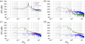
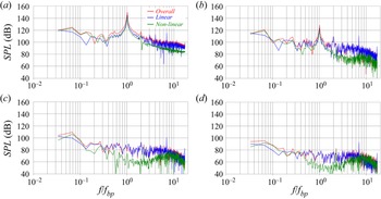
The direct approach to the hydroacoustic analysis by means of (2.5) gave us also the opportunity to distinguish between linear and nonlinear sources of noise. A comparison between them is reported in figure 24. In figure 24(a) the hydrophone at  $r/D=0.58$ and
 $z/D=0.0$ is considered. The main contribution is provided by the linear sources, although that from the nonlinear sources is non-negligible, especially in the range of very low frequencies. Already at
 $r/D=0.58$ and
 $z/D=0.5$ in figure 24(b) the change is dramatic. Although the highest frequencies are still dominated by the linear terms, the opposite is true for frequencies lower than
 $\,f_{bp}$. This trend is reinforced further downstream in figure 24(c) (
 $z/D=1.0$) and figure 24(d) (
 $z/D=2.0$), where the quadrupole terms become the leading ones across all frequencies. This result is in agreement with the theoretical analysis recently reported by Ianniello & De Bernardis (Reference Ianniello and De Bernardis2015) and Ianniello (Reference Ianniello2016), indicating the importance of the volume terms in the hydroacoustics of marine propellers. Figure 24 agrees also with the findings reported from RANS computations in the earlier studies by Ianniello et al. (Reference Ianniello, Muscari and Di Mascio2013, Reference Ianniello, Muscari and Di Mascio2014). However, they acknowledged that RANS, damping the nonlinear sources and unable to reproduce the instability phenomena affecting the wake development, was likely to underestimate the importance of the quadrupole terms in defining the acoustic signature of marine propellers. The results shown in figure 24 are also consistent with this conclusion: due to wake instability the noise from the nonlinear sources, especially at low frequencies, experiences even a rise, in contrast with that from the loading and thickness terms.
SPLs at hydrophones placed at the radial coordinate  $r/D=0.58$ and the streamwise coordinates (a)
 $z/D=0.0$, (b)
 $z/D=0.5$, (c)
 $z/D=1.0$ and (d)
 $z/D=2.0$: comparison between linear and nonlinear sources of noise.

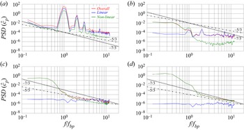
The decomposition between linear and nonlinear components is represented also in terms of PSDs, to clarify the source of the  $-$5/3 behaviour observed above in figure 22 within the inertial range of frequencies. The results in figure 25 are straightforward in demonstrating that the
 $-$5/3 slope comes from the nonlinear sources, because they are those associated with the turbulent structures populating the wake. In figure 25(a), dealing with the coordinates
 $r/D=0.58$ and
 $z/D=0.0$, the tonal noise is still dominant, on both linear and nonlinear components, so the spectra deviate from both
 $-$5/3 and
 $-$7/3 slopes. In the region of development of instability of the wake system, energising substantially the smallest frequencies, the slope of PSD still departs significantly from that of Kolmogorov's theory, as shown in figure 25(b). However, eventually the process of turbulent energy cascade towards smaller scales leads to the spectra in figure 25(c) (
 $z/D=1.0$), where the nonlinear component of sound, which became by far the dominant one, develops the
 $-$5/3 slope at the highest frequencies. This trend is reinforced further downstream at
 $z/D=2.0$, as shown in figure 25(d). As expected, the behaviour at the lowest frequencies, which is tied to phenomena of wake meandering, the dynamics of the largest structures and coupling between them, keeps far from that of the homogeneous, isotropic turbulence. Instead, moving towards larger frequencies the agreement with Kolmogorov's slope improves substantially. It is also worth noting that actually in figure 25 only the smallest frequencies of the acoustic signature of the propeller are included, due to the storage limitations associated with the sampling frequency during the LES computations.
PSD of  $\hat {c}_p$ at hydrophones placed at the radial coordinate
 $r/D=0.58$ and the streamwise coordinates (a)
 $z/D=0.0$, (b)
 $z/D=0.5$, (c)
 $z/D=1.0$ and (d)
 $z/D=2.0$: comparison between linear and nonlinear sources of noise. Dotted-dashed and dashed lines are for the slopes in the inertial range of frequencies for velocity and hydrodynamic pressure, respectively, from Kolmogorov's theory on homogeneous, isotropic turbulence.

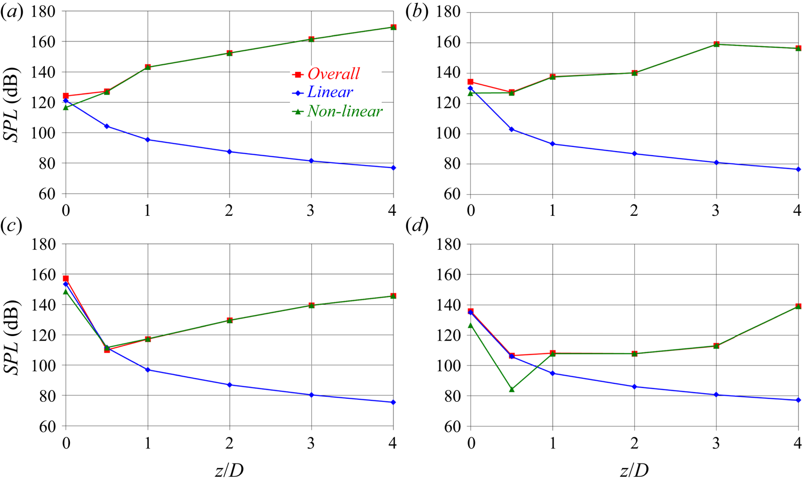
The results of figure 24 are summarised, considering the SPLs in one-third octave bands. Figure 26 deals with the same frequencies considered in figure 23. Over the propeller plane ( $z/D=0.0$) the linear component of the SPL is higher than the nonlinear component at all frequencies, although the two contributions are actually quite close. This is obviously not the case anymore at downstream locations, where the linear component experiences a substantial decay, whereas the opposite occurs for the nonlinear component. In particular, for the smallest frequencies, already at
 $z/D=0.5$ the SPLs are largely dominated by the nonlinear sources and the linear sources become negligible, as shown in both figures 26(a) and 26(b). At higher frequencies (figure 26c,d) this ‘transition’ is slower. However, already at
 $z/D = 1.0$ most sound comes from the quadrupole terms.
Streamwise evolution of the SPLs in one-third octave bands at the radial location  $r/D=0.58$ and the frequencies (a)
 $f/f_{bp}=0.25$, (b)
 $f/f_{bp}=0.50$, (c)
 $f/f_{bp}=1.00$ and (d)
 $f/f_{bp}=2.00$: comparison between linear and nonlinear sources of noise.

An advantage of the direct approach to the exploitation of the FWH acoustic analogy consists in the possibility of computing the terms contributing to the SPLs in different regions of the computational domain. The results of this ‘decomposition’ provide a clue about the flow structures having the most significant role in defining the acoustic signature. A similar strategy was adopted by Keller et al. (Reference Keller, Kumar and Mahesh2018) and Cianferra et al. (Reference Cianferra, Petronio and Armenio2019b), although in the former case only the linear terms of the acoustic signature were computed. Following this approach we considered three different regions of the overall cylindrical domain of integration. The inner region goes from the wake axis to the radial coordinate  $r/D=0.15$. This is roughly the radial size of the hub of the propeller. The middle region is defined between
 $0.15 < r/D < 0.35$, and is placed in the wake of the propeller blades. The outer region,
 $0.35 < r/D < 0.56$, is that populated by the tip vortices. As discussed by Posa et al. (Reference Posa, Broglia, Felli, Falchi and Balaras2019b), they experience a shift towards inner radial coordinates, due to the wake contraction produced by the acceleration of the flow by the propeller.
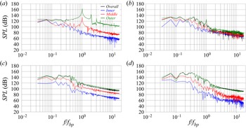
The SPLs in figure 24 coming from nonlinear sources were computed in the inner, middle and outer regions of the propeller wake and visualised in figure 27, together with the overall sound from nonlinear sources across the whole propeller wake. In all cases the major contribution comes by the outer region, populated by the tip vortices. It should be acknowledged that this result is certainly affected by the strong dependence of the sound from nonlinear sources on the distance of the hydrophones. These are closer to the outer boundary of the wake than to the wake axis, therefore the former has a more significant effect on the SPLs than the latter. In figure 27(a) the lead of the sound from the outer region is especially evident at the highest frequencies. However, it should be noted that this result is likely due to the outer region of the shear layer shed from the trailing edge of the propeller blades, rather than to the tip vortices, because they are still very stable and coherent at the considered streamwise location, resulting in large SPLs at the frequency of the blade passage and its harmonics. It is also interesting to see that the outer region of the propeller wake is that experiencing the most evident non-monotonic streamwise evolution. From  $z/D=0.0$ to
 $z/D=0.5$ a decrease occurs at the highest frequencies, which is the result of the decline of the turbulence levels in the wake of each propeller blade, affecting especially the frequency of the blade passage in both outer and middle regions. This is not the case in the inner wake, where the SPLs increase, although they are still lower than those in the middle and outer regions. In contrast, the SPLs in the middle and outer wakes rise between
 $z/D=0.5$ and
 $z/D=1.0$, which is the region where the influence by the hub vortex is felt at outer radial coordinates and the breakup of the tip vortices undergoes an acceleration. Further downstream at
 $z/D = 2.0$ the low-frequency noise in the outer region increases, as the process of instability of the tip vortices generates phenomena of mutual inductance, meandering and coupling between them (Felli et al. Reference Felli, Camussi and Di Felice2011).
SPLs at hydrophones placed at the radial coordinate  $r/D=0.58$ and the streamwise coordinates (a)
 $z/D=0.0$, (b)
 $z/D=0.5$, (c)
 $z/D=1.0$ and (d)
 $z/D=2.0$: comparison between nonlinear sources of noise from the inner (
 $r/D<0.15$), middle (
 $0.15< r/D<0.35$) and outer (
 $0.35< r/D<0.56$) regions of the propeller wake.

The hydrodynamic analysis of the flow downstream of the propeller demonstrated that its wake is initially quite stable. Between  $z/D=0.5$ and
 $z/D=1.0$ the instantaneous fluctuations of the tip and hub vortices around their mean trajectories grow significantly, energising the lowest frequencies. The tip vortices start breaking up into smaller structures, which is likely to be a reason for the increasing high-frequency noise. Meanwhile the PSD of the acoustic pressure approaches the expected trend from Kolmogorov's theory, as we found at downstream hydrophones. In contrast, the hub vortex remains coherent further downstream, but extending its signature up to outer radii, triggering the development of large fluctuations around the wake axis, further energising the range of low frequencies. This wake dynamics was also found in agreement with the earlier experimental study on the INSEAN E779A marine propeller reported by Felli et al. (Reference Felli, Camussi and Di Felice2011).
4.2.3. Radial evolution of the acoustic signature
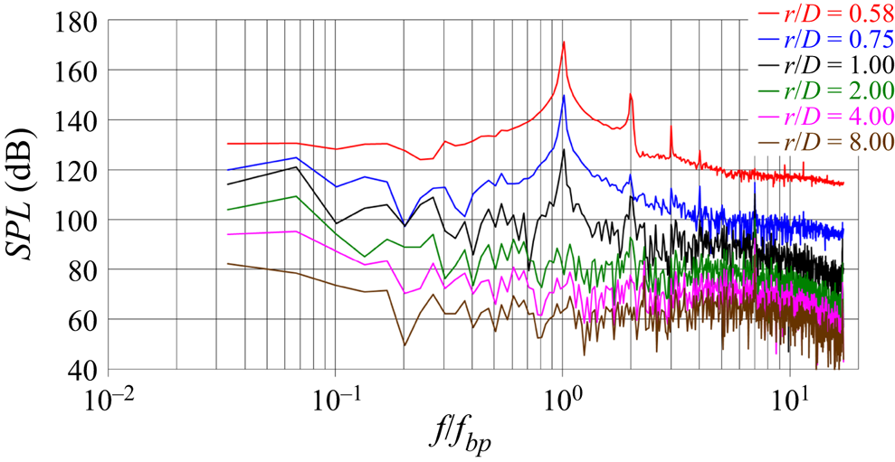
The radial evolution of the SPLs is reported in figure 28. In this case the hydrophones share the same streamwise position at  $z/D=0.0$ and are located at
 $r/D=0.58$,
 $r/D=0.75$,
 $r/D=1.0$,
 $r/D=2.0$,
 $r/D=4.0$ and
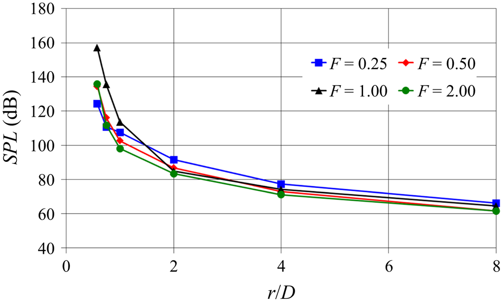
 $r/D=8.0$. The comparison with figure 21 reveals important differences. SPLs drop substantially across all frequencies. The results in figure 21 show that the instability of the wake, developing along the streamwise direction, promotes a streamwise increase. In contrast, moving away from the propeller along the radial direction results in a decline of the acoustic signature.
SPLs at hydrophones placed at the axial coordinate  $z/D=0.0$ across six radial locations, ranging from
 $r/D=0.58$ to
 $r/D=8.00$.

The results in figure 28 were computed in one-third octave bands and reported in figure 29. Although the acoustic signature is tonal in the vicinity of the propeller, this is increasingly not the case moving away along the radial direction. The spectra in figure 28 become indeed more homogeneous across frequencies as the hydrophones are shifted away from the propeller.
Radial evolution of the SPLs in one-third octave bands at the streamwise location  $z/D=0.0$ across four values of non-dimensional frequency
 $F=f/f_{bp}$.

In this case we also extended our analysis distinguishing at each hydrophone the contributions from the linear and the nonlinear sources and results are significantly different from those in figure 24. Figure 30(a) deals with the hydrophone at  $r/D=0.75$. Although around the frequency of the blade passage the noise from linear and nonlinear sources is similar, at the lowest frequencies the main contribution is from the latter and at the highest frequencies from the former. However, moving away from the propeller the range of frequencies dominated by the monopole and dipole terms becomes wider, as demonstrated by the other panels of figure 30. The comparison with the results reported in § 4.2.2 reveals that, without the contribution by the nonlinear sources associated with the wake instability, the linear terms of the FWH equation get the upper hand moving away from the propeller, whereas the opposite trend was found along the streamwise direction, that is the direction of wake development.
SPLs at hydrophones placed at the axial coordinate  $z/D=0.0$ and the radial coordinates (a)
 $r/D=0.75$, (b)
 $r/D=1.00$, (c)
 $r/D=2.00$ and (d)
 $r/D=4.00$: comparison between linear and nonlinear sources of noise.

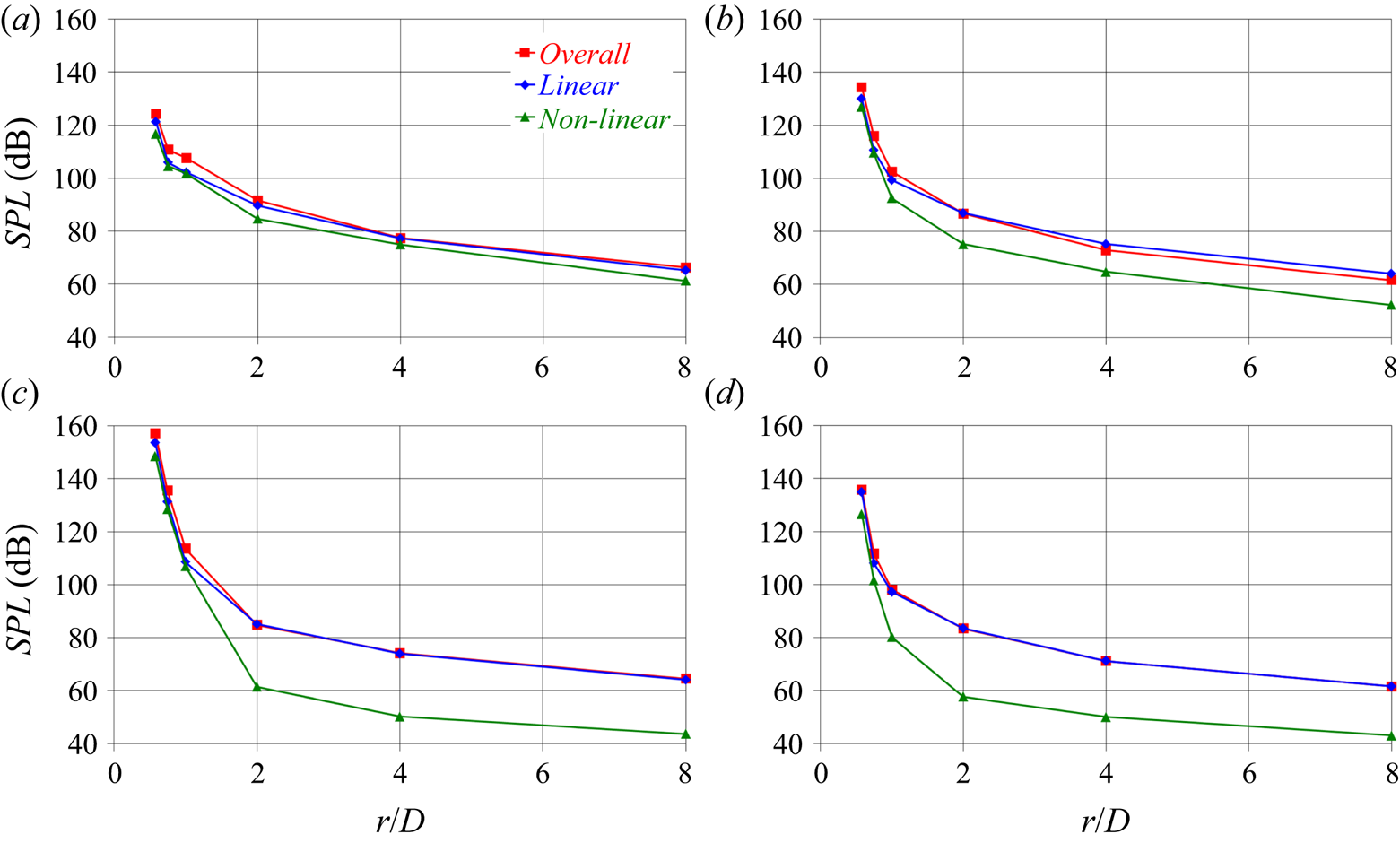
The conclusions above are summarised in figure 31, where values of SPLs in one-third octave bands are reported at selected frequencies. Figure 31(a) shows that at  $f/f_{bp}=0.25$ the decay of the linear and nonlinear sources is similar. Already at
 $f/f_{bp}=0.50$ (figure 31b) the trends are modified: the nonlinear terms are experiencing a faster decline, in comparison with the linear ones. This behaviour is reinforced at
 $f/f_{bp}=1.00$ and
 $f/f_{bp}=2.00$, as illustrated in the panels of figures 31(c) and 31(d), respectively. As a result, the linear sources, which are already more significant than the nonlinear ones in the vicinity of the propeller at
 $r/D=0.58$, become increasingly the leading ones as one moves away along the radial direction. The results in figure 31 point out that this phenomenon is especially evident around the frequency of the blade passage.
Radial evolution of the SPLs in one-third octave bands at the streamwise location  $z/D=0.0$ and the frequencies (a)
 $f/f_{bp}=0.25$, (b)
 $f/f_{bp}=0.50$, (c)
 $f/f_{bp}=1.00$ and (d)
 $f/f_{bp}=2.00$: comparison between linear and nonlinear sources of noise.

5. Conclusions
The acoustic signature of a submarine propeller has been analysed relying on the acoustic analogy. The direct approach to the computation of all terms of the integral form of the FWH equation has been utilised. The analysis was based on high-fidelity LES computations, validated in an earlier study against PIV measurements in the propeller wake (Posa et al. Reference Posa, Broglia, Felli, Falchi and Balaras2019b).
The results of this study demonstrated that the acoustic signature of the propeller decays along the radial direction, with the linear terms keeping the dominant source of noise on the propeller plane. This was found to not be the case along the streamwise direction, that is the direction of wake development. The quadrupole terms, associated with the wealth of structures shed by the propeller and their instabilities, became quickly the major source of acoustic pressure. In particular, we found that, although the linear terms faced the expected decay moving away from the propeller plane, this was not the case for the nonlinear terms. The latter experienced even an increase, involving initially the lowest frequencies and then spreading also to the highest frequencies. The instability of the tip vortices was likely accelerated by the low-frequency oscillations of the hub vortex around the wake axis, leading to break-up into smaller structures and feeding the process of turbulent energy cascade, promoting this way also an increase of the acoustic signature at higher frequencies. The resulting behaviour of the acoustic pressure in the range of inertial frequencies was found in line with that of turbulent velocity fluctuations expected from Kolmogorov's theory on homogeneous, isotropic turbulence.
This study was verified in very close agreement with the theoretical studies recently reported by Ianniello & De Bernardis (Reference Ianniello and De Bernardis2015) and Ianniello (Reference Ianniello2016): in the hydroacoustics of marine propellers the role of the quadrupole terms cannot be neglected. Instead, they become quickly the dominant source of noise at downstream locations, at least at radial coordinates in the vicinity of the propeller wake. This conclusion was found also in general agreement with the earlier study by Cianferra et al. (Reference Cianferra, Petronio and Armenio2019b), who verified a faster decay of the sound from linear sources. In fact, the present analysis demonstrated that the development of wake instability is even able to reinforce the acoustic pressure associated with the nonlinear sources at some distance from the wake generator, depending on the size/intensity of the coherent structures it sheds. Although Cianferra et al. (Reference Cianferra, Petronio and Armenio2019b) considered a marine propeller in pull configuration, here a more realistic push configuration was simulated. This set-up allowed the generation of a large hub vortex, which was actually verified the coherent structure dominating the wake dynamics and the acoustic signature of the propeller downstream of the break-up of the tip vortices.
Funding
The authors wish to thank Drs K.-H. Kim and E. McCarthy of the Office of Naval Research and Office of Naval Research Global for their support through NICOP grant N62909-19-1-2001. This study was funded in part by the European Union's Horizon 2020 research and innovation programme under grant agreement N. 101006443 (SATURN, Developing solutions for underwater radiated noise). We are grateful to Michael Brown (Naval Surface Warfare Center, Carderock Division, Maryland), for generating the Lagrangian grid of the INSEAN E1658 propeller and to Massimiliano Guarrasi (CINECA) for his support for access to HPC resources. We acknowledge PRACE for awarding us access to Marconi KNL at CINECA, Italy, with an allocation granted to the project ‘High Fidelity LES on High Skewed Propellers with Upstream Disturbances’ (project no. 2016163889) in the framework of the 15th PRACE Call for Proposals for Project Access.
Declaration of interests
The authors report no conflict of interest.