1 Introduction
Multigrid methods are among the most efficient numerical methods for solving large-scale systems of equations – linear and non-linear alike – arising from the discretization of partial differential equations. These types of methods can be viewed as an acceleration of traditional iterative methods based on local relaxation, such as Gauss–Seidel and Jacobi methods. For linear systems arising from finite element or finite difference discretization of elliptic boundary value problems, local relaxation methods were observed to converge very rapidly for the high-frequency part of the solution. The low-frequency part of the solution, although slow to converge, corresponds to a relatively smooth part of the function that can be well approximated on a coarser grid. The main idea behind such multigrid methods is to project the error obtained after applying a few iterations of local relaxation methods onto a coarser grid. The projected error equations have two characteristics. First, the resulting system is smaller. Second, part of the slowly converging low-frequency error on a finer grid becomes relatively high-frequency on the coarser grid, and these frequencies can be further corrected via a local relaxation method, but this time on the coarse grid. By repeating this process via ever coarser grids, a multilevel iterative process is obtained. Such algorithms have been proved to have uniform convergence with nearly optimal complexity for a large class of linear algebraic systems arising from the discretization of partial differential equations, especially elliptic boundary problems of second and fourth order. One main component of this type of multilevel algorithm is a hierarchy of geometric grids, typically a sequence of nested grids obtained by successive refinement. The resulting algorithms are known as geometric multigrid (GMG) methods.
Despite their extraordinary efficiency, however, GMG methods have limitations. They depend on a hierarchy of geometric grids, which is often not readily available, and it can be argued that the range of applicability of GMG methods is therefore limited.
Algebraic multigrid (AMG) methods were designed in an attempt to address such limitations. They were proposed as a means to generalize geometric multigrid methods for systems of equations that share properties with discretized PDEs, such as the Laplacian equation, but potentially have unstructured grids in the underlying discretization. The first AMG algorithm in Brandt, McCormick and Ruge (Reference Brandt, Mccormick and Ruge1982) was a method developed under the assumption that such a problem was being solved. The AMG algorithm was later generalized using several heuristics to extend its applicability to more general problems and matrices. As a result, a variety of AMG methods have been developed in the past three decades, and they have been successfully applied to many practical problems.
In this paper we give an overview of AMG methods from a theoretical viewpoint. AMG methods have been developed via a combination of certain theoretical considerations and heuristic arguments, and many AMG methods work, with varying efficiency, for different applications. We find it very hard to give a coherent picture of the state of the art of AMG methods by simply choosing to make a comprehensive list of existing algorithms without digging into their theoretical foundations. Unfortunately, a good theoretical understanding of how and why these methods work is still seriously lacking.
In preparing this paper, we have undertaken the task of making a thorough investigation into the design and analysis of AMG from a theoretical point of view. While there are many bits and pieces of ideas diffused in the literature, we have managed to re-examine most of the existing results and ‘re-invent the wheel’ in trying to deliver a coherent theoretical description. To do this, we have developed several tools for the design and analysis of AMG.
With very few exceptions, most AMG algorithms have targeted the solution of symmetric positive definite (SPD) systems. In this paper we choose to present our studies for a slightly larger class of problems, namely symmetric positive semi-definite (SPSD) systems. This approach is not only more inclusive, but more importantly, the SPSD class of linear systems can be viewed as more intrinsic to AMG ideas. For example, while the standard discretizations of the Laplacian operator with homogeneous Dirichlet boundary conditions results in an SPD system, the design of AMG may be better understood by using local problems (defined on subdomains) with homogeneous Neumann boundary conditions, yielding SPSD sub-systems.
In short, in this paper we consider AMG techniques for solving the linear system of equations
 $$\begin{eqnarray}Au=f,\end{eqnarray}$$
where
 $A$
is a given SPSD operator or sparse matrix, and the problem is posed in a vector space of large dimension. The starting point of an AMG procedure is first to choose a smoother, which is often taken to be some local relaxation iterative method such as pointwise Jacobi or Gauss–Seidel, or, more generally, overlapping Schwarz methods. The use of pointwise smoothers seems to encompass most of the efforts in the literature to construct and implement most (if not all) AMG methods. More general smoothers based on overlapping Schwarz methods are necessary for some problems, but we shall not study them in detail in this paper. In any event, any chosen smoother is expected to converge well only on certain components of the solution, which will be known as algebraic high frequencies with respect to the given smoother. With the smoother fixed, the main task of an AMG method is then to identify a sequence of coarse spaces that would complement this smoother well. Roughly speaking, an ideal sequence of coarse spaces is such that any vector (namely the solution to (1.1) for any
 $f$
) in the finest space can be well represented by a linear combination of all the algebraic high frequencies on all coarse spaces. As a result, the AMG method would converge well for problem (1.1).
It is hard to translate the above multilevel setting into a concise mathematical statement. Instead we will focus on first answering this question for a two-level setting. For a two-level setting, the first theoretical question is as follows: ‘Given a smoother, say
 $R$
, what is the optimal coarse space of given dimension such that the resulting AMG has the best convergence rate?’ This question will be thoroughly addressed in Section 5. As it turns out, the optimal coarse space will consist of the eigenvectors corresponding to the lower end of the spectrum of a matrix such as
 $RA$
. While our two-level theory is theoretically pleasing, it does not offer a practical solution, as finding these eigenvectors would be too expensive. Thus, the task of the AMG design is to find a good but inexpensive approximation of this algebraic low-frequency eigenspace that will still result in an AMG algorithm with desirable convergence properties. We call such an approximation of an optimal coarse space a ‘quasi-optimal’ coarse space.
In the design of all these AMG algorithms, one key component is the coarsening of spaces via the graph associated with the matrix
 $A$
. The two main strategies are based on independent sets and on aggregation. We will present several approaches to the construction of quasi-optimal coarse spaces. We would especially advocate two approaches that have sound theoretical foundations. The first approach is outlined in Section 5 and later on in Section 11. We will first prove that the optimal coarse space from the theory in Section 5 can be characterized, in a mathematically equivalent manner, by solutions to a trace-minimization problem. In a functional setting, such a trace-minimization can be interpreted as minimization of the sum of the energy norms of a set of coarse basis functions. These precise equivalents give very clear guidance as to how some AMG methods can be constructed. One practical approach based on such a theorem is to look for energy-minimization basis functions among locally supported function classes. The resulting algorithms are known as energy-min AMG. Other AMG methods, such as classical AMG and aggregation-based AMG, can be viewed as approximations to energy-min AMG. The second approach is outlined in Section 6. The main idea is to construct a quasi-optimal coarse space by piecing together the low-end eigenspaces of some appropriately defined local operators or matrices. This approach can be used to provide quasi-optimal coarse spaces for various AMG methods, including the standard geometric multigrid method, classical AMG, energy-minimization AMG, unsmoothed and smoothed aggregation AMG, and spectral AMGe. As a simple example, this method relies on the fact that an
 $n_{c}=Jm$
-dimensional low-end eigenspace of an operator can be well approximated by gluing together
 $J$
-pieces of
 $m$
-dimensional low-end eigenspaces, for some carefully chosen local operators. Here
 $m$
is a very small integer, for example,
 $m=1$
for the Laplacian operator and
 $m=3$
(resp.
 $m=6$
) for the two-dimensional (resp. three-dimensional) linear elasticity operator. This important property of eigenspaces is closely related to Weyl’s lemma on the asymptotic behaviour of eigenvalues for elliptic boundary value problems, discussed in Section 2.3.
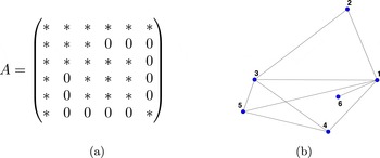
Most AMG methods are designed in terms of the adjacency graph of the coefficient matrix of a given linear algebraic system. In Section 7 we give a brief description of graph theory and the adjacency graph of a sparse matrix. One highlight of Section 7 is the concept of
 $M$
-matrix relatives. This simple tool is instrumental in the design and analysis of the classical AMG method.
One important step in the design of most AMG methods is to zero out some entries of the coefficient matrix
 $A$
by using the concept of connection strength to construct a filtered matrix
 $\tilde{A}$
, which is equivalent to omitting weakly connected edges in the adjacency graph
 ${\mathcal{G}}(A)$
to obtain
 ${\mathcal{G}}(\tilde{A})$
. Several possible strength functions are introduced in Section 8 to describe the connection strength. In Section 9, the graph
 ${\mathcal{G}}(\tilde{A})$
is then coarsened by either keeping a maximal independent set (MIS) as a coarse vertex set
 ${\mathcal{C}}$
and then dropping the rest of grid, or using aggregation/agglomeration. In Section 9 we also give some technical details of the construction of a coarse space by using degrees of freedom.
By using the aforementioned general approaches and theoretical techniques, we then motivate and present a number of AMG methods. Some of the highlights of the paper are outlined below.
We first give an overview of GMG and its relationship with AMG in Section 10. After describing some details of a typical GMG method for linear finite element matrix, we argue that the geometric information used in defining a GMG is essentially the graph information of the underlying finite element grid (without using other geometric information such as coordinates of the grid points). This is a strong indication that at least some GMG methods can be realized in a purely algebraic fashion, using only the stiffness matrix, an algebraic smoother, and the adjacency graph of the stiffness matrix. On the other hand, we prove that a GMG method can also be formally obtained via our general AMG approach, presented in Section 6. Furthermore, we use the example of AMGe in Section 10.4 to demonstrate that geometric information on the grid can be used effectively to construct a geometry-based AMG.
In Section 11 we give a detailed account of AMG methods based on energy-minimization. We first present our new theory that the optimal coarse space shown in the two-level theory in Section 5 can actually be obtained by trace-minimization (Section 11.1), after which we derive the energy-min AMG method by seeking a set of locally supported coarse basis functions for energy-minimization.
Classical AMG, as the first class of AMG algorithms studied in the literature, will be presented in Section 12. We derive and analyse this type of method using the framework in Section 6 together with the notion of
 $M$
-matrix relatives introduced in Section 7.2. We further discuss how a classical AMG method can be viewed as an approximation of the energy-min AMG method.
Aggregation-based AMG will be presented in Section 13. Again we derive and analyse this method using the framework in Section 6. One remarkable feature of aggregation AMG methods is their ease at preserving multi-dimensional near-null spaces, such as rigid body modes in linear elasticity.
To demonstrate how an AMG method addresses possible heterogeneous properties in a given problem, we devote Section 14 to showing how classical AMG is designed to address the difficulties arising from discretized elliptic problems with strong discontinuous jumps, or anisotropy in the coefficients of the underlying PDE.
In Section 15 we outline a class of AMG methods that attempt to choose the coarse spaces in a bootstrap and adaptive fashion. This class of AMG algorithms does not fall within the theoretical frameworks presented in this paper, but they provide a practical approach to generalizing many existing AMG techniques to more general problems. Finally we make some concluding remarks in Section 16.
We conclude these introductory remarks with a brief summary of the acronyms used for the various AMG algorithms reviewed in this paper.

2 Model problems and discretization
While AMG has found applications to a wide range of linear algebraic systems, its development has been mainly motivated by the solution of systems arising from the discretization of partial differential equations by finite element, finite difference or other numerical methods. In this section we will discuss a model of second-order elliptic boundary problems, their finite difference and finite element discretization, and relevant properties of the underlying differential operators and their discretization.
2.1 Model elliptic PDE operators
We consider the boundary value problems
 $$\begin{eqnarray}{\mathcal{L}}u=-\unicode[STIX]{x1D6FB}\cdot \unicode[STIX]{x1D6FC}(x)\unicode[STIX]{x1D6FB}u=f,\quad x\in \unicode[STIX]{x1D6FA},\end{eqnarray}$$
where
 $\unicode[STIX]{x1D6FC}:\unicode[STIX]{x1D6FA}\mapsto \mathbb{R}^{d\times d}$
is an SPD matrix function satisfying
 $$\begin{eqnarray}\unicode[STIX]{x1D6FC}_{0}\Vert \unicode[STIX]{x1D709}\Vert ^{2}\leq \unicode[STIX]{x1D709}^{T}\unicode[STIX]{x1D6FC}(x)\unicode[STIX]{x1D709}\leq \unicode[STIX]{x1D6FC}_{1}\Vert \unicode[STIX]{x1D709}\Vert ^{2},\quad \unicode[STIX]{x1D709}\in \mathbb{R}^{d},\end{eqnarray}$$
for some positive constants
 $\unicode[STIX]{x1D6FC}_{0}$
and
 $\unicode[STIX]{x1D6FC}_{1}$
. Here
 $d=1,2,3$
, and
 $\unicode[STIX]{x1D6FA}\subset \mathbb{R}^{d}$
is a bounded domain with boundary
 $\unicode[STIX]{x1D6E4}=\unicode[STIX]{x2202}\unicode[STIX]{x1D6FA}$
.
A variational formulation for (2.1) is as follows: find
 $u\in V$
such that
 $$\begin{eqnarray}a(u,v)=(f,v),\quad \text{for all}~v\in V.\end{eqnarray}$$
Here
 $$\begin{eqnarray}a(u,v)=\int _{\unicode[STIX]{x1D6FA}}(\unicode[STIX]{x1D6FC}(x)\unicode[STIX]{x1D6FB}u)\cdot \unicode[STIX]{x1D6FB}v,\quad (f,v)=\int _{\unicode[STIX]{x1D6FA}}fv,\end{eqnarray}$$
and
 $V$
is a Sobolev space that can be chosen to address different boundary conditions accompanying equation (2.1). One case is that of mixed boundary conditions
 $$\begin{eqnarray}\begin{array}{@{}rll@{}}u & =0, & x\in \unicode[STIX]{x1D6E4}_{D},\\ (\unicode[STIX]{x1D6FC}\unicode[STIX]{x1D6FB}u)\cdot n & =0, & x\in \unicode[STIX]{x1D6E4}_{N},\end{array}\end{eqnarray}$$
where
 $\unicode[STIX]{x1D6E4}=\unicode[STIX]{x1D6E4}_{D}\cup \unicode[STIX]{x1D6E4}_{N}$
. The pure Dirichlet problem is when
 $\unicode[STIX]{x1D6E4}_{D}=\unicode[STIX]{x1D6E4}$
, while the pure Neumann problem is when
 $\unicode[STIX]{x1D6E4}_{N}=\unicode[STIX]{x1D6E4}$
. We thus have
 $V$
as
 $$\begin{eqnarray}V=\left\{\begin{array}{@{}l@{}}H^{1}(\unicode[STIX]{x1D6FA})=\{v\in L^{2}(\unicode[STIX]{x1D6FA}):\unicode[STIX]{x2202}_{i}v\in L^{2}(\unicode[STIX]{x1D6FA}),i=1:d\},\\ H_{D}^{1}(\unicode[STIX]{x1D6FA})=\{v\in H^{1}(\unicode[STIX]{x1D6FA}):v|_{\unicode[STIX]{x1D6E4}_{D}}=0\}.\end{array}\right.\end{eqnarray}$$
When we consider a pure Dirichlet problem,
 $\unicode[STIX]{x1D6E4}_{D}=\unicode[STIX]{x1D6E4}$
, we denote the space by
 $V=H_{0}^{1}(\unicode[STIX]{x1D6FA})$
. In addition, for pure Neumann boundary conditions, the following condition is added to ensure the existence of the solution to (2.3):
 $$\begin{eqnarray}\int _{\unicode[STIX]{x1D6FA}}f=0.\end{eqnarray}$$
One of the most commonly used model problems is when
 $$\begin{eqnarray}\unicode[STIX]{x1D6FC}(x)=1,\quad x\in \unicode[STIX]{x1D6FA},\end{eqnarray}$$
which corresponds to the Poisson equation
 $$\begin{eqnarray}-\unicode[STIX]{x1D6E5}u=f.\end{eqnarray}$$
This simple problem provides a good representative model for isotropic problems.
There are two other cases that are of special interest. The first case is when
 $\unicode[STIX]{x1D6FC}$
is a scalar and has discontinuous jumps such as
 $$\begin{eqnarray}\unicode[STIX]{x1D6FC}(x)=\left\{\begin{array}{@{}ll@{}}\unicode[STIX]{x1D716}\quad & x\in \unicode[STIX]{x1D6FA}_{1},\\ 1\quad & x\in \unicode[STIX]{x1D6FA}_{2}.\end{array}\right.\end{eqnarray}$$
The second case is when
 $\unicode[STIX]{x1D6FC}$
is a diagonal matrix such as (for
 $d=2$
)
 $$\begin{eqnarray}\unicode[STIX]{x1D6FC}(x)=\left(\begin{array}{@{}cc@{}}1 & 0\\ 0 & \unicode[STIX]{x1D716}\end{array}\right)\!,\end{eqnarray}$$
which corresponds to the operator
 $$\begin{eqnarray}-u_{xx}-\unicode[STIX]{x1D716}u_{yy}=f.\end{eqnarray}$$
In both cases we assume that
 $\unicode[STIX]{x1D716}$
is sufficiently small to investigate the robustness of algorithms with respect to discontinuous jumps and anisotropy.
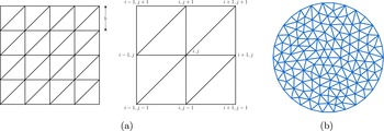
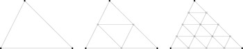
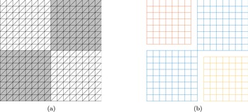
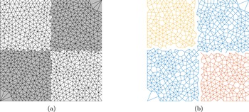
(a) Regular (uniform) triangulations for the unit square, and (b) unstructured mesh approximating the unit disk.

2.2 Examples of finite difference and finite element discretizations
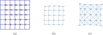
As an illustrative example, we consider a finite difference discretization of the Poisson equation (2.8) with pure Dirichlet boundary conditions on the unit square
 $\unicode[STIX]{x1D6FA}=(0,1)\times (0,1)$
. We consider a uniform triangulation of
 $\unicode[STIX]{x1D6FA}$
(see Figure 2.1(a)), and we set
 $$\begin{eqnarray}(x_{i},y_{j})=\biggl(\displaystyle \frac{i}{n+1},\displaystyle \frac{j}{n+1}\biggr),\quad u_{i,j}\approx u(x_{i},y_{j}),\quad (i,j=0,\ldots ,n+1).\end{eqnarray}$$
We use the standard central difference approximation to the Laplacian operator
 $$\begin{eqnarray}(-\unicode[STIX]{x1D6E5}u)(x_{i},y_{j})\approx \displaystyle \frac{4u_{i,j}-u_{i+1,j}-u_{i-1,j}-u_{i,j+1}-u_{i,j-1}}{h^{2}}.\end{eqnarray}$$
The finite difference scheme is then given by
 $$\begin{eqnarray}4u_{i,j}-(u_{i+1,j}+u_{i-1,j}+u_{i,j+1}+u_{i,j-1})=h^{2}f_{i,j},\end{eqnarray}$$
where
 $$\begin{eqnarray}f_{i,j}=f(x_{i},y_{j})\end{eqnarray}$$
and
 $u_{i,j}\approx u(x_{i},y_{j})$
. The approximations
 $u_{i,j}$
are found by solving a linear system. We order the points
 $(x_{i},y_{j})$
lexicographically, and for
 $k=1,\ldots ,n^{2}$
we have
 $$\begin{eqnarray}k=(j-1)n+i,\quad x_{k}^{h}=(x_{i},y_{j}),\quad \unicode[STIX]{x1D707}_{k}=u_{i,j},\quad 1\leq i,j\leq n,\end{eqnarray}$$
We can then write (2.12) as
 $$\begin{eqnarray}A\unicode[STIX]{x1D707}=b,\end{eqnarray}$$
where
 $$\begin{eqnarray}A=\operatorname{tridiag}(-I,B,-I)\quad \text{and}\quad B=\operatorname{tridiag}(-1,4,-1).\end{eqnarray}$$
A slightly different scheme is obtained using more of the neighbouring points of
 $(x_{i},y_{j})$
. We can build an approximation using 8 points
 $(x_{i\pm 1},y_{j\pm 1})$
together with the ‘centre’ point
 $(x_{i},y_{j})$
. As a result we have the following 9-point finite difference scheme:
 $$\begin{eqnarray}\displaystyle & 8\unicode[STIX]{x1D707}_{i,j}-\unicode[STIX]{x1D707}_{i-1,j}-\unicode[STIX]{x1D707}_{i+1,j}-\unicode[STIX]{x1D707}_{i,j-1}-\unicode[STIX]{x1D707}_{i,j+1} & \displaystyle \nonumber\\ \displaystyle & \qquad \phantom{8\unicode[STIX]{x1D707}_{i,j}}-\unicode[STIX]{x1D707}_{i-1,j-1}-\unicode[STIX]{x1D707}_{i+1,j-1}-\unicode[STIX]{x1D707}_{i-1,j+1}-\unicode[STIX]{x1D707}_{i+1,j+1}=2h^{2}f_{i,j}. & \displaystyle\end{eqnarray}$$
Again, if we order
 $(x_{i},y_{j})$
lexicographically, then (2.17) is the linear system (2.15) corresponding to the 9-point finite difference discretization of the Laplace equation, where
 $$\begin{eqnarray}A=\operatorname{tridiag}(-C,B,-C),\quad B=\operatorname{tridiag}(-1,8,-1),~C=\operatorname{tridiag}(1,1,1).\end{eqnarray}$$
We now give an example of finite element discretization. Given a triangulation
 ${\mathcal{T}}_{h}$
for
 $\unicode[STIX]{x1D6FA}$
, such as that given in Figure 2.1, let
 $V_{h}\subset V$
be a finite element space consisting of piecewise linear (or higher-order) polynomials with respect to the triangulation
 ${\mathcal{T}}_{h}$
. The finite element approximation of the variational problem (2.3) is: find
 $u_{h}\in V_{h}$
such that
 $$\begin{eqnarray}a(u_{h},v_{h})=(f,v_{h}),\quad \text{for all}~\,v_{h}\in V_{h}.\end{eqnarray}$$
Assume
 $\{\unicode[STIX]{x1D719}_{i}\}_{i=1}^{N}$
is the nodal basis of
 $V_{h}$
, namely
 $\unicode[STIX]{x1D719}_{i}(x_{j})=\unicode[STIX]{x1D6FF}_{ij}$
for any nodes
 $x_{j}$
. We write
 $u_{h}(x)=\sum _{j=1}^{N}\unicode[STIX]{x1D707}_{j}\unicode[STIX]{x1D719}_{j}(x)$
. Equation (2.19) is then equivalent to
 $$\begin{eqnarray}\mathop{\sum }_{j=1}^{N}\unicode[STIX]{x1D707}_{j}a(\unicode[STIX]{x1D719}_{j},\unicode[STIX]{x1D719}_{i})=(f,\unicode[STIX]{x1D719}_{i}),\quad j=1,2,\ldots ,N,\end{eqnarray}$$
which is a linear system of equations:
 $$\begin{eqnarray}A\unicode[STIX]{x1D707}=b,\quad (A)_{ij}=a(\unicode[STIX]{x1D719}_{j},\unicode[STIX]{x1D719}_{i})\quad \text{and}\quad (b)_{i}=(f,\unicode[STIX]{x1D719}_{i}).\end{eqnarray}$$
The matrix
 $A$
is known as the stiffness matrix of the nodal basis
 $\{\unicode[STIX]{x1D719}_{i}\}_{i=1}^{N}$
.
For
 $d=2$
and the special uniform triangulation shown in Figure 2.1, this stiffness matrix for the Laplacian operator turns out to be exactly the one given by (2.12). This special case is an example of the close relationship between finite difference and finite element methods.
We note that the finite element method is based on the variational formulation (2.3), whereas the finite difference method is not. In the development of the AMG method, however, the variational method is also used to derive coarse level equations for finite difference methods.
For any
 $T\in {\mathcal{T}}_{h}$
, we define
 $$\begin{eqnarray}\overline{h}_{T}=\text{diam}(T),\quad h_{T}=|T|^{1/d},\quad \text{}\underline{h}_{T}=2\sup \{r>0:B(x,r)\subset T\text{ for }x\in T\}.\end{eqnarray}$$
We say that the mesh
 ${\mathcal{T}}_{h}$
is shape-regular if there exists a uniformly bounded constant
 $\unicode[STIX]{x1D70E}\geq 1$
such that
 $$\begin{eqnarray}\text{}\underline{h}_{T}\leq h_{T}\leq \overline{h}_{T}\leq \unicode[STIX]{x1D70E}\text{}\underline{h}_{T},\quad \text{for all}~T\in {\mathcal{T}}_{h}.\end{eqnarray}$$
We call
 $\unicode[STIX]{x1D70E}$
the shape-regularity constant.
Let
 $h=\max _{T\in {\mathcal{T}}_{h}}\overline{h}_{T}$
, with
 $\overline{h}_{T}$
defined as in (2.21). We say that the mesh
 ${\mathcal{T}}_{h}$
is quasi-uniform if there exists a uniformly bounded constant
 $C>0$
such that
 $$\begin{eqnarray}\displaystyle \frac{h}{\text{}\underline{h}_{T}}\leq C.\end{eqnarray}$$
2.3 Spectral properties
We now discuss the spectral properties of the partial differential operator
 ${\mathcal{L}}$
given in (2.1).
We recall the well-known Courant–Fischer min-max principle (Courant and Hilbert Reference Courant and Hilbert1924) for eigenvalues of symmetric matrices.
Theorem 2.1. Let
 $T$
be an
 $n\times n$
symmetric matrix with respect to
 $(\cdot ,\cdot )_{\ast }$
, and let
 $\{\unicode[STIX]{x1D706}_{j},\unicode[STIX]{x1D701}_{j}\}$
be its eigenpairs with
 $\unicode[STIX]{x1D706}_{1}\leq \unicode[STIX]{x1D706}_{2}\leq \cdots \leq \unicode[STIX]{x1D706}_{n}$
. Then
 $$\begin{eqnarray}\unicode[STIX]{x1D706}_{k}=\min _{\dim W=k}\max _{x\in W,x\neq 0}\displaystyle \frac{(Tx,x)_{\ast }}{(x,x)_{\ast }},\end{eqnarray}$$
where the minimum is achieved if
 $$\begin{eqnarray}W=\operatorname{span}\{\unicode[STIX]{x1D701}_{j}:j=1:k\},\end{eqnarray}$$
and
 $$\begin{eqnarray}\unicode[STIX]{x1D706}_{k}=\max _{\dim W=n-k+1}\min _{x\in W,x\neq 0}\displaystyle \frac{(Tx,x)_{\ast }}{(x,x)_{\ast }},\end{eqnarray}$$
where the maximum is achieved if
 $$\begin{eqnarray}W=\operatorname{span}\{\unicode[STIX]{x1D701}_{j}:j=k:n\}.\end{eqnarray}$$
Next, we recall Theorem 1 in Fan (Reference Fan1949), which is known as the Ky–Fan trace-minimization principle.
Theorem 2.2. We assume
 $T$
is symmetric with respect to
 $(\cdot ,\cdot )_{\ast }$
, and
 $\{\unicode[STIX]{x1D706}_{j},\unicode[STIX]{x1D701}_{j}\}$
are its eigenpairs with
 $\unicode[STIX]{x1D706}_{1}\leq \unicode[STIX]{x1D706}_{2}\leq \cdots \leq \unicode[STIX]{x1D706}_{n}$
. Then
 $$\begin{eqnarray}\min _{P\in \mathbb{R}^{n\times k},P^{\ast }P=I}\operatorname{trace}(P^{\ast }TP)=\mathop{\sum }_{j=1}^{k}\unicode[STIX]{x1D706}_{j}.\end{eqnarray}$$
Furthermore, the minimum is achieved when
 $$\begin{eqnarray}\operatorname{range}(P)=\operatorname{span}\{\unicode[STIX]{x1D701}_{j}\}_{j=1}^{k}\quad \text{and}\quad P^{\ast }P=I.\end{eqnarray}$$
Here
 $P^{\ast }\in \mathbb{R}^{k\times n}$
is the adjoint of
 $P$
with respect to the
 $(\cdot ,\cdot )_{\ast }$
-inner product, namely
 $$\begin{eqnarray}(P^{\ast }u,v)=(u,Pv)_{\ast },\quad \text{for all }u\in \mathbb{R}^{n},~v\in \mathbb{R}^{k}.\end{eqnarray}$$
Finally, following Xu (Reference Xu1992), we use the notation
 $a\lesssim b$
to represent the existence of a generic positive constant
 $C$
, which is independent of salient parameters, such as problem size or anisotropic ratio, and such that
 $a\leq Cb$
. Furthermore, we write
 $a{\displaystyle\mathop{=}\limits_{{\sim}}}b$
if and only if
 $a\lesssim b$
and
 $b\lesssim a$
.
Theorem 2.3. The PDE operator
 ${\mathcal{L}}$
has a complete set of eigenfunctions
 $(\unicode[STIX]{x1D711}_{k})$
and non-negative eigenvalues
 $$\begin{eqnarray}0\leq \unicode[STIX]{x1D706}_{1}\leq \unicode[STIX]{x1D706}_{2}\leq \cdots\end{eqnarray}$$
such that
 $$\begin{eqnarray}{\mathcal{L}}\unicode[STIX]{x1D711}_{k}=\unicode[STIX]{x1D706}_{k}\unicode[STIX]{x1D711}_{k},\quad k=1,2,3\ldots ,\end{eqnarray}$$
where
-
(a)
 $\lim _{k\rightarrow \infty }\unicode[STIX]{x1D706}_{k}=\infty ,$
-
(b)
$(\unicode[STIX]{x1D711}_{i})$
forms an orthonormal basis of
$V$
as well as for
$L^{2}(\unicode[STIX]{x1D6FA})$
.



Furthermore,
-
(c) for the pure Neumann problem,
$\unicode[STIX]{x1D706}_{1}\!=0$
, and
$\unicode[STIX]{x1D711}_{1}$
is the constant function,


-
(d) for the pure Dirichlet problem,
$\unicode[STIX]{x1D706}_{1}\!>0$
is simple, and
$\unicode[STIX]{x1D711}_{1}$
does not change sign.


We have the well-known Weyl estimate for the asymptotic behaviour of the Laplacian operator (Weyl Reference Weyl1911, Reference Weyl1912, Reed and Simon Reference Reed and Simon1978).
Lemma 2.4 (Weyl’s law).
Assume that
 $\unicode[STIX]{x1D6FA}$
is ‘contented’, which means that
 $\unicode[STIX]{x1D6FA}$
can be approximated by unions of cubes in
 $\mathbb{R}^{d}$
; see Reed and Simon (Reference Reed and Simon1978, p. 271) for the exact definition. For the homogeneous Dirichlet boundary condition, the eigenvalues of the pure Laplacian operator satisfy
 $$\begin{eqnarray}\lim _{k\rightarrow \infty }\displaystyle \frac{\unicode[STIX]{x1D706}_{k}}{k^{2/d}}=w_{\unicode[STIX]{x1D6FA}},\quad \text{with }w_{\unicode[STIX]{x1D6FA}}=\displaystyle \frac{(2\unicode[STIX]{x1D70B})^{2}}{[\unicode[STIX]{x1D714}_{d}\operatorname{Vol}(\unicode[STIX]{x1D6FA})]^{2/d}},\end{eqnarray}$$
where
 $\unicode[STIX]{x1D714}_{d}$
is the volume of the unit ball in
 $\mathbb{R}^{d}$
, and the eigenvalues of the operator
 ${\mathcal{L}}$
given in (2.1) satisfy
 $$\begin{eqnarray}\unicode[STIX]{x1D706}_{k}{\displaystyle\mathop{=}\limits_{{\sim}}}k^{2/d},\quad \text{for all}~k\geq 1.\end{eqnarray}$$
Next, we extend Weyl’s law to discretized PDE operators. The following theorem gives a discrete version of Weyl’s law for finite element discretization. Further details of this result can be found in Xu, Zhang and Zikatanov (Reference Xu, Zhang and Zikatanov2016b ).
Theorem 2.5. Let
 $V_{h}\subset H_{0}^{1}(\unicode[STIX]{x1D6FA})$
be a family of finite element spaces on a quasi-uniform mesh with
 $\dim V_{h}=N$
. Consider the discretized operator of (2.1),
 $$\begin{eqnarray}{\mathcal{L}}_{h}:V_{h}\mapsto V_{h},\quad ({\mathcal{L}}_{h}u,v)=a(u,v),\quad \text{for all}~u,v\in V_{h},\end{eqnarray}$$
and its eigenvalues,
 $$\begin{eqnarray}\unicode[STIX]{x1D706}_{h,1}\leq \unicode[STIX]{x1D706}_{h,2}\leq \cdots \leq \unicode[STIX]{x1D706}_{h,N}.\end{eqnarray}$$
Then, for all
 $1\leq k\leq N$
, there exists a constant
 $C_{w}>0$
independent of
 $k$
such that we have the estimates
 $$\begin{eqnarray}\unicode[STIX]{x1D706}_{k}\leq \unicode[STIX]{x1D706}_{h,k}\leq C_{w}\unicode[STIX]{x1D706}_{k}\end{eqnarray}$$
and
 $$\begin{eqnarray}\unicode[STIX]{x1D706}_{h,k}{\displaystyle\mathop{=}\limits_{{\sim}}}k^{2/d}.\end{eqnarray}$$
2.4 Properties of finite element matrices
The main algebraic property for the stiffness matrices given by (2.20) is that it is sparse with
 $O(N)$
non-zeros, symmetric positive definite (for both Dirichlet and mixed boundary conditions) and semi-definite for pure Neumann boundary conditions. Its eigenvalues satisfy a discrete Weyl’s law.
For simplicity, we will only consider pure Dirichlet boundary conditions in the rest of this section.
Lemma 2.6. The stiffness matrix
 $A$
given by (2.20) has the following properties.
-
(a) The condition number of
$A$
, defined by the ratio of the extreme eigenvalues of
$A$
, satisfies
$$\begin{eqnarray}\unicode[STIX]{x1D705}(A)=\displaystyle \frac{\unicode[STIX]{x1D706}_{\max }(A)}{\unicode[STIX]{x1D706}_{\min }(A)},\end{eqnarray}$$
Furthermore,
$$\begin{eqnarray}\unicode[STIX]{x1D705}(A){\displaystyle\mathop{=}\limits_{{\sim}}}h^{-2}.\end{eqnarray}$$
$$\begin{eqnarray}\unicode[STIX]{x1D706}_{\min }(A){\displaystyle\mathop{=}\limits_{{\sim}}}h^{2}\quad \text{and}\quad \unicode[STIX]{x1D706}_{ max}(A){\displaystyle\mathop{=}\limits_{{\sim}}}1.\end{eqnarray}$$
-
(b) The discrete version of Weyl’s law holds:
$$\begin{eqnarray}\unicode[STIX]{x1D706}_{k}(A){\displaystyle\mathop{=}\limits_{{\sim}}}\biggl(\displaystyle \frac{k}{N}\biggr)^{2/d}.\end{eqnarray}$$


We next discuss some more refined spectral properties of finite element stiffness matrices from uniform grids for the unit square domain
 $\unicode[STIX]{x1D6FA}=(0,1)\times (0,1)$
for
 $d=2$
. We begin with the Poisson equation. It is easy to derive a closed-form solution of the eigenpairs of
 $A$
given by (2.15), and we have
 $$\begin{eqnarray}\unicode[STIX]{x1D706}_{kl}(A)=4\biggl(\sin ^{2}\displaystyle \frac{k\unicode[STIX]{x1D70B}}{2(n+1)}+\sin ^{2}\displaystyle \frac{l\unicode[STIX]{x1D70B}}{2(n+1)}\biggr)\end{eqnarray}$$
and
 $$\begin{eqnarray}\unicode[STIX]{x1D719}_{ij}^{kl}=\sin \displaystyle \frac{ki\unicode[STIX]{x1D70B}}{n+1}\sin \displaystyle \frac{lj\unicode[STIX]{x1D70B}}{n+1},\quad 1\leq i\leq n,~1\leq j\leq n.\end{eqnarray}$$
Now consider the important case of anisotropic problem (2.11). We order the vertices of the triangulation lexicographically, and, as before, denote them by
 $\{(ih,jh)\}_{i,j=0}^{n}$
. The stiffness matrix is then
 $$\begin{eqnarray}A=\operatorname{tridiag}(-I,B,-I)\quad \text{with }B=\operatorname{tridiag}(-\unicode[STIX]{x1D716},2(1+\unicode[STIX]{x1D716}),-\unicode[STIX]{x1D716}).\end{eqnarray}$$
Obviously,
 $$\begin{eqnarray}A=I\otimes B+C\otimes I\quad \text{with }C=\operatorname{tridiag}(-1,0,-1),\end{eqnarray}$$
and it is easily verified that
 $$\begin{eqnarray}\unicode[STIX]{x1D706}_{i}(B)=2(1+\unicode[STIX]{x1D716})-2\unicode[STIX]{x1D716}\cos \displaystyle \frac{i\unicode[STIX]{x1D70B}}{(n+1)},\quad \unicode[STIX]{x1D706}_{j}(C)=-2\cos \displaystyle \frac{j\unicode[STIX]{x1D70B}}{(n+1)},\quad 1\leq i,j\leq N.\end{eqnarray}$$
which leads to the expression
 $$\begin{eqnarray}\unicode[STIX]{x1D706}_{ij}(A)=4\unicode[STIX]{x1D716}\sin ^{2}\displaystyle \frac{i\unicode[STIX]{x1D70B}}{2(n+1)}+4\sin ^{2}\displaystyle \frac{j\unicode[STIX]{x1D70B}}{2(n+1)}\end{eqnarray}$$
for the eigenvalues, and
 $$\begin{eqnarray}\unicode[STIX]{x1D719}_{ij}^{k\ell }=\sin \displaystyle \frac{ki\unicode[STIX]{x1D70B}}{n+1}\sin \displaystyle \frac{\ell j\unicode[STIX]{x1D70B}}{n+1}\end{eqnarray}$$
for the corresponding eigenvectors.
3 Linear vector spaces and duals
In this paper we will mainly consider linear systems of equations of the form
 $$\begin{eqnarray}Au=f.\end{eqnarray}$$
Here
 $$\begin{eqnarray}A:V\mapsto V^{\prime },\end{eqnarray}$$
 $$\begin{eqnarray}\quad f\in V^{\prime },\end{eqnarray}$$
where
 $V$
is a finite-dimensional linear vector space and
 $V^{\prime }$
is the dual of
 $V$
. If we use the notation
 $\langle \cdot ,\cdot \rangle$
to denote the pairing between
 $V^{\prime }$
and
 $V$
, we can write (3.1) in a variational form: find
 $u\in V$
such that
 $$\begin{eqnarray}a(u,v)=\langle f,v\rangle ,\quad \text{for all}~v\in V,\end{eqnarray}$$
where
 $$\begin{eqnarray}a(u,v)=\langle Au,v\rangle .\end{eqnarray}$$
3.1 Dual and inner product
For convenience of exposition, we will assume that
 $V$
is equipped with an inner product
 $(\cdot ,\cdot )$
. By the Riesz representation theorem, for any
 $f\in V^{\prime }$
, there is a unique
 $u\in V$
such that
 $$\begin{eqnarray}(u,v)=\langle f,v\rangle ,\quad \text{for all}~v\in V.\end{eqnarray}$$
It is via the Riesz representation theorem that we identify the dual space
 $V^{\prime }$
with
 $V$
. In the rest of this paper, for convenience, we will always assume that
 $V^{\prime }=V$
for any finite-dimensional vector space
 $V$
. As a result, we have
 $$\begin{eqnarray}V^{\prime \prime }=(V^{\prime })^{\prime }=V^{\prime }=V.\end{eqnarray}$$
Thanks to the identification
 $V^{\prime }=V$
via (3.5), the identities in (3.6) are clear.
We would like to point out that, in an abstract discussion of all iterative methods for problem (3.1), it suffices to use the abstract dual pairing
 $\langle \cdot ,\cdot \rangle$
without having to introduce an inner product
 $(\cdot ,\cdot )$
on
 $V$
. However, we find that using an inner product is convenient for exposition, as we shall see later. We further point out that we will not use an inner product to identify
 $V^{\prime }=V$
for any infinite-dimensional vector space in this paper.
If
 $\{\unicode[STIX]{x1D719}_{i}\}_{i=1}^{N}$
is a basis of
 $V$
, we will always choose a basis
 $\{\unicode[STIX]{x1D713}_{i}\}_{i=1}^{N}$
of
 $V^{\prime }$
that is dual to the basis of
 $V$
, namely
 $$\begin{eqnarray}(\unicode[STIX]{x1D713}_{j},\unicode[STIX]{x1D719}_{i})=\unicode[STIX]{x1D6FF}_{ij},\quad 1\leq i,~j\leq N.\end{eqnarray}$$
Such a dual basis will be used only for theoretical considerations and not for the actual implementation of any algorithms.
We will consider two kinds of linear vector spaces. The first kind is
 $V=\mathbb{R}^{n}$
and the inner product is just the dot product
 $$\begin{eqnarray}(u,v)_{\ell ^{2}}=\mathop{\sum }_{i=1}^{n}u_{i}v_{i},\quad \text{for all}~u=(u_{i}),~v=(v_{i})\in \mathbb{R}^{n},\end{eqnarray}$$
A canonical basis of
 $\mathbb{R}^{N}$
is formed by the column vectors of the identity matrix,
 $\{e_{i}\}_{i=1}^{N}$
. It is easy to see that the dual basis of
 $(\mathbb{R}^{N})^{\prime }=\mathbb{R}^{N}$
is just the original basis
 $\{e_{i}\}_{i=1}^{N}$
itself.
The second kind is a finite-dimensional functional subspace of
 $L^{2}(\unicode[STIX]{x1D6FA})$
for a given domain
 $\unicode[STIX]{x1D6FA}\subset \mathbb{R}^{d}$
(
 $1\leq d\leq 3$
), equipped with the
 $L^{2}$
-inner product
 $$\begin{eqnarray}(u,v)=\int _{\unicode[STIX]{x1D6FA}}u(x)v(x).\end{eqnarray}$$
One commonly used linear vector space is a finite element space
 $V_{h}$
, and the nodal basis functions
 $\{\unicode[STIX]{x1D719}_{i}\}_{i=1}^{N}$
are often used as a basis. In this case, the dual basis functions
 $\{\unicode[STIX]{x1D713}_{i}\}_{i=1}^{N}$
of
 $V^{\prime }$
are no longer the original nodal basis functions but rather a set of functions (which are usually globally supported) that satisfy (3.7). This set of dual basis functions is usually needed to derive the matrix representation of operators between various spaces and their duals, but they are not needed for the actual implementation of relevant algorithms.
For a linear operator
 $$\begin{eqnarray}L:V\mapsto V,\end{eqnarray}$$
its adjoint,
 $$\begin{eqnarray}L^{\prime }:V\mapsto V,\end{eqnarray}$$
is defined as follows:
 $$\begin{eqnarray}(L^{\prime }u,v)=(u,Lv),\quad u,v\in V.\end{eqnarray}$$
Since
 $V$
plays the role of both
 $V$
and its dual
 $V^{\prime }$
, (3.8) and (3.9) can have four different meanings:
-
(i) if
$L:V\mapsto V$
, then
$L^{\prime }:V^{\prime }\mapsto V^{\prime }$
, -
(ii) if
$L:V\mapsto V^{\prime }$
, then
$L^{\prime }:V\mapsto V^{\prime }$
, -
(iii) if
$L:V^{\prime }\mapsto V$
, then
$L^{\prime }:V^{\prime }\mapsto V$
, -
(iv) if
$L:V^{\prime }\mapsto V^{\prime }$
, then
$L^{\prime }:V\mapsto V$
.


Thanks to the identification we made between
 $V^{\prime }$
and
 $V$
via (3.5), definition (3.10) is applicable to all four cases.
If
 $V=\mathbb{R}^{n}$
and
 $(u,v)=(u,v)_{\ell ^{2}}$
, then
 $L^{\prime }=L^{T}$
, namely the matrix transpose. We say that an operator
 $A:V\mapsto V^{\prime }$
is symmetric positive definite (SPD) if
 $$\begin{eqnarray}A^{\prime }=A,\quad (Av,v)>0,\quad \text{for all}~v\in V\setminus \{0\}.\end{eqnarray}$$
When
 $A$
is SPD, it defines another inner product
 $(\cdot ,\cdot )_{A}$
on
 $V$
,
 $$\begin{eqnarray}(u,v)_{A}=(Au,v),\quad u,v\in V,\end{eqnarray}$$
and a corresponding norm,
 $$\begin{eqnarray}\Vert v\Vert _{A}=(v,v)_{A}^{1/2},\quad v\in V.\end{eqnarray}$$
We use the superscript ‘*’ for the adjoint operator with respect to
 $(\cdot ,\cdot )_{A}$
, that is,
 $$\begin{eqnarray}(Bu,v)_{A}=(u,B^{\ast }v)_{A}.\end{eqnarray}$$
It is easy to see that
 $$\begin{eqnarray}(BA)^{\ast }=B^{\prime }A,\end{eqnarray}$$
and
 $(BA)^{\ast }=BA$
if and only if
 $B^{\prime }=B$
.
3.2 Matrix representation
Let
 $V_{c}\subset V$
be a subspace and consider the inclusion operator
 $\imath _{c}:V_{c}\mapsto V$
. Assume that
 $\{\unicode[STIX]{x1D719}_{i}^{c}\}_{i=1}^{n_{c}}$
and
 $\{\unicode[STIX]{x1D719}_{i}\}_{i=1}^{n}$
are basis functions of
 $V_{c}$
and
 $V$
respectively, and the matrix representation of
 $\imath _{c}$
is the matrix
 $$\begin{eqnarray}P:\mathbb{R}^{n_{c}}\mapsto \mathbb{R}^{n}\text{ satisfying }(\unicode[STIX]{x1D719}_{1}^{c},\ldots ,\unicode[STIX]{x1D719}_{n_{c}}^{c})=(\unicode[STIX]{x1D719}_{1},\ldots ,\unicode[STIX]{x1D719}_{n})P.\end{eqnarray}$$
Equation (3.12) is shorthand for the expansion of the basis in
 $V_{c}$
via the basis in
 $V$
:
 $$\begin{eqnarray}\unicode[STIX]{x1D719}_{k}^{c}=\mathop{\sum }_{j=1}^{n}p_{jk}\unicode[STIX]{x1D719}_{j},\quad P=(p_{jk}),\quad k=1,\ldots ,n_{c},~j=1,\ldots ,n.\end{eqnarray}$$
What is the matrix representation of
 $\imath _{c}^{\prime }:V^{\prime }\mapsto V_{c}^{\prime }$
? Although we have
 $V^{\prime }=V$
and
 $V_{c}^{\prime }=V_{c}$
, we need to use dual bases
 $\{\unicode[STIX]{x1D713}_{i}^{c}\}_{i=1}^{n_{c}}\subset V_{c}^{\prime }$
and
 $\{\unicode[STIX]{x1D713}_{i}\}_{i=1}^{n}\subset V^{\prime }$
respectively. With respect to these dual bases, the matrix representation of
 $\imath _{c}^{\prime }$
is simply
 $P^{T}$
(the transpose of
 $P$
), since it is easy to verify that
 $$\begin{eqnarray}(\imath _{c}^{\prime }\unicode[STIX]{x1D713}_{1},\ldots ,\imath _{c}^{\prime }\unicode[STIX]{x1D713}_{n})=(\unicode[STIX]{x1D713}_{1}^{c},\ldots ,\unicode[STIX]{x1D713}_{n_{c}}^{c})P^{T}.\end{eqnarray}$$
Now consider a linear operator
 $$\begin{eqnarray}A:V\mapsto V.\end{eqnarray}$$
There are two different ways to get a matrix representation of
 $A$
, because
 $V$
plays two roles here:
 $V$
is
 $V$
itself, and
 $V=V^{\prime }$
. For the first case, we use the same basis
 $\{\unicode[STIX]{x1D719}_{i}\}$
for
 $V$
as the domain of
 $A$
and
 $V$
as the range of
 $A$
. In this case, the matrix representation of
 $A$
is the matrix
 $$\begin{eqnarray}\hat{A}\in \mathbb{R}^{n\times n}\text{ satisfying }(A\unicode[STIX]{x1D719}_{1},\ldots ,A\unicode[STIX]{x1D719}_{n})=(\unicode[STIX]{x1D719}_{1},\ldots ,\unicode[STIX]{x1D719}_{n})\hat{A}.\end{eqnarray}$$
In the second case, we use the basis
 $\{\unicode[STIX]{x1D719}_{i}\}$
for
 $V$
as the domain space of
 $A$
, but use the dual basis
 $\{\unicode[STIX]{x1D713}_{i}\}$
for
 $V^{\prime }=V$
as the range space of
 $A$
. In this case, the matrix representation of
 $A$
is the matrix
 $$\begin{eqnarray}\tilde{A}\in \mathbb{R}^{n\times n}\text{ satisfying }(A\unicode[STIX]{x1D719}_{1},\ldots ,A\unicode[STIX]{x1D719}_{n})=(\unicode[STIX]{x1D713}_{1},\ldots ,\unicode[STIX]{x1D713}_{n})\tilde{A}.\end{eqnarray}$$
It is easy to see that
 $$\begin{eqnarray}\tilde{A}=((A\unicode[STIX]{x1D719}_{j},\unicode[STIX]{x1D719}_{i}))\end{eqnarray}$$
and
 $$\begin{eqnarray}\tilde{A}=M\hat{A},\quad M=((\unicode[STIX]{x1D719}_{j},\unicode[STIX]{x1D719}_{i})).\end{eqnarray}$$
The matrix
 $\tilde{A}$
in (3.17) is often called the stiffness matrix of
 $A$
and the matrix
 $M$
in (3.18) is called the mass matrix.
In the early multigrid literature, a discrete inner product equivalent to the
 $L^{2}$
-inner product was often introduced for finite element spaces so that the corresponding mass matrix becomes diagonal. However, if we view the underlying finite element operator (3.14) in a slightly different way,
 $$\begin{eqnarray}A:V\mapsto V^{\prime },\end{eqnarray}$$
we will then see easily that the introduction of the discrete
 $L^{2}$
-inner product is not necessary.
If
 $V=\mathbb{R}^{n}$
and we choose the canonical basis
 $\{e_{i}\}$
for
 $V$
, we would not encounter the mass matrix problem as in the functional space case, since in this case
 $\{e_{i}\}$
is also the dual basis of
 $V^{\prime }$
. This is certainly convenient, but the convenience tends to mask some subtle but important difference between various vectors and matrices in a given problem and the objects (functions) that they represent.
Given a matrix
 $A\in \mathbb{R}^{n\times n}$
, we can view it as either
 $$\begin{eqnarray}A:\mathbb{R}^{n}\mapsto \mathbb{R}^{n}\end{eqnarray}$$
or
 $$\begin{eqnarray}A:\mathbb{R}^{n}\mapsto (\mathbb{R}^{n})^{\prime }.\end{eqnarray}$$
As it turns out, when
 $A$
is obtained from the discretization of partial differential equations, (3.21) is more informative than (3.20). Hence we write a matrix equation
 $$\begin{eqnarray}Ax=b.\end{eqnarray}$$
It is sometimes helpful to regard
 $x$
and
 $b$
as living in two ‘different’ spaces,
 $$\begin{eqnarray}x\in \mathbb{R}^{n}\quad \text{and}\quad b\in (\mathbb{R}^{n})^{\prime }.\end{eqnarray}$$
3.3 Eigenvalues and eigenvectors
Let us briefly discuss eigenvalues and eigenvectors for the symmetric operator
 $T:V\mapsto V$
. If
 $(\unicode[STIX]{x1D706},\unicode[STIX]{x1D719})$
is an eigenpair of
 $T$
,
 $$\begin{eqnarray}T\unicode[STIX]{x1D719}=\unicode[STIX]{x1D706}\unicode[STIX]{x1D719},\end{eqnarray}$$
then it is easy to see that
 $(\unicode[STIX]{x1D706},\tilde{\unicode[STIX]{x1D719}})$
is an eigenpair of the matrix representation
 $\tilde{T}$
of
 $T$
:
 $$\begin{eqnarray}\tilde{T}\tilde{\unicode[STIX]{x1D719}}=\unicode[STIX]{x1D706}\tilde{\unicode[STIX]{x1D719}}.\end{eqnarray}$$
Here
 $\tilde{\unicode[STIX]{x1D719}}\in \mathbb{R}^{n}$
is the vector representation of
 $\unicode[STIX]{x1D719}$
:
 $$\begin{eqnarray}\unicode[STIX]{x1D719}=(\unicode[STIX]{x1D719}_{1},\ldots ,\unicode[STIX]{x1D719}_{n})\tilde{\unicode[STIX]{x1D719}}.\end{eqnarray}$$
For an operator
 $A$
defined in (3.14), we need to be cautious when talking about eigenvalues of
 $A$
. Although we identify
 $V^{\prime }=V$
via (3.5),
 $V^{\prime }$
and
 $V$
play two different roles, so
 $A$
is essentially a mapping between two ‘different’ spaces
 $V$
and
 $V^{\prime }$
, and the spectrum of
 $A$
should be defined carefully. However, if we consider a symmetric operator
 $$\begin{eqnarray}R:V^{\prime }\mapsto V,\end{eqnarray}$$
then
 $RA:V\mapsto V$
is an operator that is symmetric with respect to the
 $A$
-inner product. In this case, if
 $(\unicode[STIX]{x1D706},\unicode[STIX]{x1D719})$
is an eigenpair of
 $RA$
, then
 $(\unicode[STIX]{x1D706},\tilde{\unicode[STIX]{x1D719}})$
is an eigenpair of
 $\tilde{R}\tilde{A}$
(i.e. equal to the matrix representation of
 $RA$
).
We consider the trivial identification operator
 $$\begin{eqnarray}\jmath :V^{\prime }\mapsto V\text{ such that }\jmath \unicode[STIX]{x1D713}_{i}=\unicode[STIX]{x1D713}_{i},~\text{for all}~i,\end{eqnarray}$$
namely
 $\jmath v=v$
for all
 $v\in V^{\prime }=V$
. It is easy to see that the matrix representation of
 $\jmath$
is the inverse of the mass matrix
 $M=((\unicode[STIX]{x1D719}_{j},\unicode[STIX]{x1D719}_{i}))$
, namely
 $$\begin{eqnarray}\tilde{\jmath }=M^{-1}.\end{eqnarray}$$
Using this identification operator, the operator
 $\jmath A:V\mapsto V$
is a symmetric operator from
 $V$
to
 $V$
. We can then talk about its spectrum. For example, if
 $(\unicode[STIX]{x1D706},\unicode[STIX]{x1D719})$
is an eigenpair of
 $\jmath A$
, then
 $(\unicode[STIX]{x1D706},\tilde{\unicode[STIX]{x1D719}})$
satisfies
 $$\begin{eqnarray}\tilde{A}\tilde{\unicode[STIX]{x1D719}}=\unicode[STIX]{x1D706}M\tilde{\unicode[STIX]{x1D719}}.\end{eqnarray}$$
This is often the generalized eigenvalue problem appearing in finite element analysis.
Although, for all
 $v\in V$
,
 $\jmath Av=Av$
because of the identification introduced above,
 $\jmath A$
and
 $A$
are, strictly speaking, two different operators: they have two different ranges and their matrix representations are different.
The discussions above, although simple, may seem a little confusing at first glance, but an unambiguous understanding and clarification of these concepts and the underlying subtleties will be helpful for the presentation of algebraic multigrid methods in the rest of this paper. For more detailed discussions on relevant topics, we refer to Xu (Reference Xu2016).
3.4 Bibliographical notes
For a general reading on the basic linear algebra materials used here, we refer to Halmos (Reference Halmos1974) and Xu (Reference Xu1992, Reference Xu2016). In particular, for a more detailed discussion related to dual spaces and matrix representations, we refer to Xu (Reference Xu1992, Reference Xu2016).
4 Basic iterative methods
We now consider linear iterative methods for solving (2.20). We will focus on two of the most commonly used algorithms, namely the Jacobi and Gauss–Seidel methods. Let us first give a brief introduction to linear iterative methods in a more general setting. Recall the basic problem under consideration. Given a finite-dimensional vector space
 $V$
equipped with an inner product
 $(\cdot ,\cdot )$
, we consider
 $$\begin{eqnarray}Au=f,\end{eqnarray}$$
where
 $A:V\mapsto V^{\prime }$
is symmetric positive definite (SPD) and
 $V^{\prime }$
is the dual of
 $V$
. As mentioned in Section 3, we will identify
 $V^{\prime }=V$
via an inner product
 $(\cdot ,\cdot )$
.
4.1 Basic iterative methods
A general linear iterative method for solving (4.1) can be written as follows. Given
 $u^{0}\in V$
, we define
 $$\begin{eqnarray}u^{m}=u^{m-1}+B(f-Au^{m-1}),\quad m=1,2,\ldots ,\end{eqnarray}$$
where
 $B:V^{\prime }\mapsto V$
is a linear operator which can be thought of as an approximate inverse of
 $A$
.
Sometimes it is more desirable for the iterator
 $B$
to be symmetric. If
 $B$
is not symmetric, there is a natural way to symmetrize it. Consider the following iteration:
 $$\begin{eqnarray}\left\{\begin{array}{@{}rl@{}}u^{m-1/2} & =u^{m-1}+B(f-Au^{m-1}),\\ u^{m} & =u^{m-1/2}+B^{\prime }(f-Au^{m-1/2}).\end{array}\right.\end{eqnarray}$$
The symmetrized iteration (4.3) can be written as
 $$\begin{eqnarray}u^{m}=u^{m-1}+\bar{B}(f-Au^{m-1}),\quad m=1,2,\ldots ,\end{eqnarray}$$
where
 $$\begin{eqnarray}\bar{B}=B^{\prime }+B-B^{\prime }AB,\end{eqnarray}$$
which satisfies
 $$\begin{eqnarray}I-\bar{B}A=(I-BA)^{\ast }(I-BA).\end{eqnarray}$$
Obviously,
 $\unicode[STIX]{x1D70C}(I-\bar{B}A)<0$
 $\Longleftrightarrow \bar{B}>0$
 $\Longleftrightarrow$
 $G\equiv (B^{\prime })^{-1}+B^{-1}-A>0$
.
Theorem 4.1. The following results hold.
-
(a) Equation (4.3) converges if and only if
$G>0$
, which implies that (4.2) converges. Furthermore, (4.7)
$$\begin{eqnarray}\Vert I-BA\Vert _{A}^{2}=\unicode[STIX]{x1D706}_{ max}(I-\bar{B}A)=1-\biggl(\sup _{\Vert v\Vert _{A}=1}(\bar{B}^{-1}v,v)\biggr)^{-1}.\end{eqnarray}$$
-
(b) If
$B^{\prime }=B$
,
$G>0$
if and only if (4.2) converges and, with
$\unicode[STIX]{x1D702}=\unicode[STIX]{x1D706}_{\min }(G)$
, (4.8)
$$\begin{eqnarray}\displaystyle \frac{2\unicode[STIX]{x1D702}}{\unicode[STIX]{x1D702}+1}(Bv,v)\leq (\bar{B}v,v)\leq 2(Bv,v),\quad v\in V.\end{eqnarray}$$


Remark 4.2. As an exercise, the reader may generalize Theorem 4.1 to the case when
 $A$
is SPSD.
4.2 Jacobi and Gauss–Seidel methods
For
 $A=(a_{ij})\in \mathbb{R}^{n\times n}$
, we write
 $$\begin{eqnarray}A=D+L+U,\end{eqnarray}$$
where
 $D$
is the diagonal of
 $A$
, and
 $L$
and
 $U$
are the strict lower and upper triangular parts of
 $A$
respectively.


Given
 $\unicode[STIX]{x1D714}>0$
, the (modified) Jacobi method can be written as (4.2) with
 $$\begin{eqnarray}B=\unicode[STIX]{x1D714}D^{-1}=(\unicode[STIX]{x1D714}^{-1}D)^{-1},\end{eqnarray}$$
as shown in Algorithm 1. The (modified) Gauss–Seidel method can be written as (4.2) with
 $$\begin{eqnarray}B=(\unicode[STIX]{x1D714}^{-1}D+L)^{-1},\end{eqnarray}$$
as shown in Algorithm 2.
The next result, which follows easily from Theorem 4.1, is well known.
Theorem 4.3. The modified Jacobi method converges if and only
 $$\begin{eqnarray}0<\unicode[STIX]{x1D714}<\displaystyle \frac{2}{\unicode[STIX]{x1D70C}(D^{-1}A)},\end{eqnarray}$$
and the modified Gauss–Seidel method converges if and only if
 $$\begin{eqnarray}0<\unicode[STIX]{x1D714}<2.\end{eqnarray}$$
In practice, it is often easy to choose
 $\unicode[STIX]{x1D714}$
to satisfy (4.9) so that the modified Jacobi method is guaranteed to converge. In the rest of this paper, we may always assume that such a choice of
 $\unicode[STIX]{x1D714}$
is made. For the Gauss–Seidel method, we will always choose
 $\unicode[STIX]{x1D714}=1$
(optimal successive over-relaxation is not generally used in multigrid methods). The Jacobi and Gauss–Seidel methods together with their convergence theory can be extended to block matrices in a straightforward fashion.
4.3 The subspace correction method
We consider a sequence of spaces
 $V_{1},\ldots ,V_{J}$
. These spaces, which will be known as auxiliary spaces, are not necessarily subspaces of
 $V$
, but each of them is related to the original space
 $V$
by a linear operator
 $$\begin{eqnarray}\unicode[STIX]{x1D6F1}_{k}:V_{k}\mapsto V.\end{eqnarray}$$
Our very basic assumption is that the following decomposition holds:
 $$\begin{eqnarray}V=\mathop{\sum }_{i=1}^{J}\unicode[STIX]{x1D6F1}_{i}V_{i}.\end{eqnarray}$$
This means that for any
 $v\in V$
there exists
 $v_{i}\in V_{i}$
(which may not be unique) such that
 $$\begin{eqnarray}v=\mathop{\sum }_{i=1}^{J}\unicode[STIX]{x1D6F1}_{i}v_{i}.\end{eqnarray}$$
Furthermore, we assume that each
 $V_{i}$
is equipped with an energy inner product
 $a_{i}(\cdot ,\cdot )$
. We define
 $$\begin{eqnarray}A_{i}:V_{i}\mapsto V_{i}^{\prime }\end{eqnarray}$$
by
 $$\begin{eqnarray}(A_{i}u_{i},v_{i})=a_{i}(u_{i},v_{i}),\quad u_{i},~v_{i}\in V_{i}.\end{eqnarray}$$
Let
 $\unicode[STIX]{x1D6F1}_{i}^{\prime }:V^{\prime }\mapsto V_{i}^{\prime }$
be the adjoint of
 $\unicode[STIX]{x1D6F1}_{i}$
:
 $$\begin{eqnarray}(\unicode[STIX]{x1D6F1}_{i}^{\prime }f,v_{i})=(f,\unicode[STIX]{x1D6F1}_{i}v_{i}),\quad f\in V^{\prime },~v_{i}\in V_{i}.\end{eqnarray}$$
Let
 $P_{i}=\unicode[STIX]{x1D6F1}_{i}^{\ast }:V\mapsto V_{i}$
be the adjoint of
 $\unicode[STIX]{x1D6F1}_{i}$
with respect to the A-inner products:
 $$\begin{eqnarray}(P_{i}u,v_{i})_{A_{i}}=(u,\unicode[STIX]{x1D6F1}_{i}v_{i})_{A},\quad u\in V,~v_{i}\in V_{i}.\end{eqnarray}$$
The following identity holds:
 $$\begin{eqnarray}\unicode[STIX]{x1D6F1}_{i}^{\prime }A=A_{i}P_{i}.\end{eqnarray}$$
If
 $u$
is the solution of (4.1), by (4.14), we have
 $$\begin{eqnarray}A_{i}u_{i}=f_{i},\end{eqnarray}$$
where
 $$\begin{eqnarray}u_{i}=P_{i}u,\quad f_{i}=\unicode[STIX]{x1D6F1}_{i}^{\prime }f.\end{eqnarray}$$
This equation may be regarded as the restriction of (4.1) to
 $V_{i}$
. We assume that each such
 $A_{i}$
has an approximate inverse or preconditioner:
 $$\begin{eqnarray}R_{i}:V_{i}^{\prime }\mapsto V_{i}.\end{eqnarray}$$
The parallel subspace correction (PSC for short) method is (4.2) with
 $B=B_{\operatorname{psc}}$
given by
 $$\begin{eqnarray}B_{\operatorname{psc}}=\mathop{\sum }_{i=1}^{J}\unicode[STIX]{x1D6F1}_{i}R_{i}\unicode[STIX]{x1D6F1}_{i}^{\prime }.\end{eqnarray}$$
The successive subspace correction (SSC for short) method is defined in Algorithm 3.

The algorithm is equivalent to (4.2) with
 $B=B_{\operatorname{ssc}}$
given by
 $$\begin{eqnarray}I-B_{\operatorname{ssc}}A=(I-T_{J})(I-T_{J-1})\cdots (I-T_{1}),\end{eqnarray}$$
where
 $$\begin{eqnarray}T_{i}=\unicode[STIX]{x1D6F1}_{i}R_{i}\unicode[STIX]{x1D6F1}_{i}^{\prime }A=\unicode[STIX]{x1D6F1}_{i}R_{i}A_{i}P_{i}.\end{eqnarray}$$
Theorem 4.4. Assume that all
 $R_{k}$
are SPD. Then
 $$\begin{eqnarray}(B_{\operatorname{psc}}^{-1}v,v)=\min _{\mathop{\sum }_{i}\unicode[STIX]{x1D6F1}_{i}v_{i}=v}\mathop{\sum }_{k=1}^{J}(R_{k}^{-1}v_{k},v_{k}),\end{eqnarray}$$
with the unique minimizer given by
 $$\begin{eqnarray}v_{k}^{\ast }=R_{k}\unicode[STIX]{x1D6F1}_{k}^{\prime }B_{\operatorname{ psc}}^{-1}v.\end{eqnarray}$$
Theorem 4.5. Under the assumptions given above, we obtain the identity
 $$\begin{eqnarray}\displaystyle \Vert I-B_{\operatorname{ssc}}A\Vert _{A}^{2} & = & \displaystyle \Vert (I-T_{J})(I-T_{J-1})\cdots (I-T_{1})\Vert _{A}^{2}\nonumber\\ \displaystyle \phantom{\Vert I-B_{\operatorname{ssc}}A\Vert _{A}^{2}} & = & \displaystyle 1-\displaystyle \frac{1}{1+c_{0}}\end{eqnarray}$$
 $$\begin{eqnarray}\displaystyle \phantom{\Vert I-B_{\operatorname{ssc}}A\Vert _{A}^{2}} & = & \displaystyle 1-\displaystyle \frac{1}{c_{1}}.\end{eqnarray}$$
Here
 $$\begin{eqnarray}c_{0}=\sup _{\Vert v\Vert _{A}=1}c_{0}(v),\quad c_{1}=\sup _{\Vert v\Vert _{A}=1}c_{1}(v)=1+c_{0},\end{eqnarray}$$
and, with
 $$\begin{eqnarray}w_{i}=(I-T_{i}^{-1})\unicode[STIX]{x1D6F1}_{i}v_{i}+\mathop{\sum }_{j=i+1}^{J}\unicode[STIX]{x1D6F1}_{j}v_{j},\end{eqnarray}$$
we obtain
 $$\begin{eqnarray}c_{0}(v)=\inf _{\mathop{\sum }_{i}\unicode[STIX]{x1D6F1}_{i}v_{i}=v}\mathop{\sum }_{i=1}^{J}(T_{i}\overline{T}_{i}^{-1}T_{i}^{\ast }w_{i},w_{i})_{A},\end{eqnarray}$$
and
 $$\begin{eqnarray}\displaystyle c_{1}(v) & = & \displaystyle (\overline{B}_{\operatorname{ssc}}^{-1}v,v)\nonumber\\ \displaystyle \phantom{c_{1}(v)} & = & \displaystyle \inf _{\mathop{\sum }_{i}\unicode[STIX]{x1D6F1}_{i}v_{i}=v}(\overline{T}_{i}^{-1}(\overline{T}_{i}T_{i}^{-1}\unicode[STIX]{x1D6F1}_{i}v_{i}+T_{i}^{\ast }w_{i}),(\overline{T}_{i}T_{i}^{-1}\unicode[STIX]{x1D6F1}_{i}v_{i}+T_{i}^{\ast }w_{i}))_{A}.\end{eqnarray}$$
In particular, if
 $R_{i}=A_{i}^{-1}$
, then
 $$\begin{eqnarray}c_{0}(v)=\inf _{\mathop{\sum }_{i}\unicode[STIX]{x1D6F1}_{i}v_{i}=v}\mathop{\sum }_{i=1}^{J}\biggl\|P_{i}\mathop{\sum }_{j=i+1}^{J}\unicode[STIX]{x1D6F1}_{j}v_{j}\biggr\|_{A_{i}}^{2}\end{eqnarray}$$
and
 $$\begin{eqnarray}c_{1}(v)=\inf _{\mathop{\sum }_{i}\unicode[STIX]{x1D6F1}_{i}v_{i}=v}\mathop{\sum }_{i=1}^{J}\biggl\|P_{i}\mathop{\sum }_{j=i}^{J}\unicode[STIX]{x1D6F1}_{j}v_{j}\biggr\|_{A_{i}}^{2}.\end{eqnarray}$$
Lemma 4.6. If
 $R_{k}=A_{k}^{-1}$
for all
 $k$
, and
 $V_{k}$
are subspaces of
 $V$
, then
 $$\begin{eqnarray}\displaystyle \frac{1}{4}(B_{\operatorname{psc}}^{-1}v,v)\leq (\bar{B}_{\operatorname{ ssc}}^{-1}v,v)\leq c^{\ast }(B_{\operatorname{ psc}}^{-1}v,v),\quad v\in V,\end{eqnarray}$$
where
 $$\begin{eqnarray}c^{\ast }=\max _{1\leq k\leq M}[N(k)]^{2}\text{ and }N(k)=\{j\in \{1,\ldots ,J\}:V_{j}\cap V_{k}\neq \{0\}\}.\end{eqnarray}$$
Proof. Given
 $v=\sum _{i=1}^{J}v_{i}$
, with
 $v_{i}\in V_{i}$
, it follows that
 $$\begin{eqnarray}\displaystyle \Vert v\Vert _{A}^{2} & = & \displaystyle \mathop{\sum }_{k,j=1}^{J}(v_{k},v_{j})_{A}=\mathop{\sum }_{k=1}^{J}(v_{k},v_{k})_{A}+2\mathop{\sum }_{j>k}^{J}(v_{k},v_{j})_{A}\nonumber\\ \displaystyle & = & \displaystyle -\mathop{\sum }_{k=1}^{J}(v_{k},v_{k})_{A}+2\mathop{\sum }_{j\geq k}^{J}(v_{k},v_{j})_{A}.\nonumber\end{eqnarray}$$
Thus
 $$\begin{eqnarray}\displaystyle \mathop{\sum }_{k=1}^{J}\Vert v_{k}\Vert _{A}^{2} & \leq & \displaystyle 2\mathop{\sum }_{k=1}^{J}\mathop{\biggl(v_{k},\mathop{\sum }_{j=k}^{J}v_{j}\biggr)}\nolimits_{A}=2\mathop{\sum }_{k=1}^{J}\mathop{\biggl(v_{k},P_{k}\mathop{\sum }_{j=k}^{J}v_{j}\biggr)}\nolimits_{A}\nonumber\\ \displaystyle & \leq & \displaystyle 2\biggl(\mathop{\sum }_{k=1}^{J}\Vert P_{k}\mathop{\sum }_{j=k}^{J}v_{j}\Vert _{A}^{2}\biggr)^{1/2}\biggl(\mathop{\sum }_{k=1}^{J}\Vert v_{k}\Vert _{A}^{2}\biggr)^{1/2}.\nonumber\end{eqnarray}$$
Consequently,
 $$\begin{eqnarray}\mathop{\sum }_{k=1}^{J}\Vert v_{k}\Vert _{A}^{2}\leq 4\mathop{\sum }_{k=1}^{J}\biggl\|P_{k}\mathop{\sum }_{j=k}^{J}v_{j}\biggr\|_{A}^{2}.\end{eqnarray}$$
By (4.20), (4.27) and (4.25), we have
 $$\begin{eqnarray}(B_{\operatorname{psc}}^{-1}v,v)\leq 4c_{1}(v)=4(\bar{B}_{\operatorname{ssc}}^{-1}v,v).\end{eqnarray}$$
The upper bound also follows easily. From
 $\Vert P_{k}\Vert _{A}=1$
and the Schwarz inequality, we obtain
 $$\begin{eqnarray}\displaystyle \mathop{\sum }_{k=1}^{J}\biggl\|P_{k}\mathop{\sum }_{j=k}^{J}v_{j}\biggr\|_{A}^{2} & = & \displaystyle \mathop{\sum }_{k=1}^{J}\biggl\|P_{k}\mathop{\sum }_{j\in N(k);j\geq k}v_{j}\biggr\|_{A}^{2}\nonumber\\ \displaystyle & \leq & \displaystyle \mathop{\sum }_{k=1}^{J}\biggl\|\mathop{\sum }_{j\in N(k);j\geq k}v_{j}\biggr\|_{A}^{2}\leq \mathop{\sum }_{k=1}^{J}N(k)\mathop{\sum }_{j\in N(k);j\geq k}\Vert v_{j}\Vert _{A}^{2}\nonumber\\ \displaystyle & \leq & \displaystyle \sqrt{c^{\ast }}\mathop{\sum }_{k=1}^{J}\mathop{\sum }_{j\in N(k);j\geq k}\Vert v_{j}\Vert _{A}^{2}\leq c^{\ast }\mathop{\sum }_{k=1}^{J}\Vert v_{k}\Vert _{A}^{2}.\nonumber\end{eqnarray}$$
The proof is concluded by taking the infimum over all decompositions on both sides and applying (4.27).◻
Remark 4.7. We would like to point that the estimate in (4.28) holds for anisotropic and jump coefficient problems, and the constant
 $c^{\ast }$
only depends on the ‘topology’ of the overlaps between the subspaces and does not depend on other ingredients and properties.
The Jacobi and Gauss–Seidel method can be interpreted as PSC and SSC based on the decomposition
 $$\begin{eqnarray}\mathbb{R}^{n}=\mathop{\sum }_{i=1}^{n}\text{span}\{e_{i}\},\end{eqnarray}$$
with exact subspace solves such that
 $$\begin{eqnarray}B_{\operatorname{psc}}=D^{-1},\quad B_{\operatorname{ ssc}}=(D+L)^{-1},\quad \bar{B}_{\operatorname{ ssc}}=(D+U)^{-1}D(D+L)^{-1}.\end{eqnarray}$$
By Theorem 4.5,
 $$\begin{eqnarray}c_{0}=\sup _{\Vert v\Vert _{A}=1}(D^{-1}Uv,Uv),\quad c_{1}=\sup _{\Vert v\Vert _{A}=1}(D^{-1}(D+U)v,(D+U)v).\end{eqnarray}$$
By Lemma 4.6,
 $$\begin{eqnarray}\displaystyle \frac{1}{4}(Dv,v)\leq (D^{-1}(D+U)v,(D+U)v)\leq c_{\ast }(Dv,v),\quad v\in \mathbb{R}^{n}.\end{eqnarray}$$
We note that
 $$\begin{eqnarray}c_{1}=\sup _{v\in V}\displaystyle \frac{(\bar{B}_{\operatorname{ssc}}^{-1}v,v)}{\Vert v\Vert _{A}^{2}}\leq \unicode[STIX]{x1D70E}\sup _{v\in V}\displaystyle \frac{\Vert v\Vert _{D}^{2}}{\Vert v\Vert _{A}^{2}},\end{eqnarray}$$
where
 $$\begin{eqnarray}\unicode[STIX]{x1D70E}=\sup _{v\in V}\displaystyle \frac{\Vert v\Vert _{\bar{B}_{\operatorname{ssc}}^{-1}}^{2}}{(Dv,v)}.\end{eqnarray}$$
In the above presentation, most results are for SPD problems. We would like to point out that all of these results can be extended to a more general class of problems, namely symmetric positive semi-definite problems. When
 $A$
is a matrix, we further assume that all the diagonals of
 $A$
are non-zero and hence positive. When the subspace correction method is used for a more general symmetric positive semi-definite operator
 $A$
, we further assume that each
 $A_{i}$
is SPD. We shall use the acronym SPSD to denote matrices or operators that satisfy the aforementioned properties.
4.4 Bibliographical notes
The general notion of subspace corrections by means of space decompositions was described by Xu (Reference Xu1992), based on Bramble, Pasciak, Wang and Xu (Reference Bramble, Pasciak, Wang and Xu1991b , Reference Bramble, Pasciak, Wang and Xu1991c ). It is an abstract point of view encompassing the theory and practice of a large class of iterative algorithms such as multigrid and domain decomposition methods. In the past two decades a great deal of effort has been put into the investigation of theoretical and practical issues related to these methods. General results, applicable in many cases, in the theory of additive and multiplicative methods in Hilbert space can be found in Xu and Zikatanov (Reference Xu and Zikatanov2002). For a literature review and basic results we refer the reader to the monographs and survey articles by Hackbusch (Reference Hackbusch1985), Bramble (Reference Bramble1993), Vassilevski (Reference Vassilevski2008), Xu (Reference Xu1989, Reference Xu and Ainsworth1997), Xu and Zou (Reference Xu and Zou1998), Yserentant (Reference Yserentant1993), Toselli and Widlund (Reference Toselli and Widlund2005), Griebel and Oswald (Reference Griebel and Oswald1995) and Smith, Bjørstad and Gropp (Reference Smith, Bjørstad and Gropp1996). For detailed studies of classical iterative methods, we refer to the monographs by Young (Reference Young1971), Hackbusch (Reference Hackbusch1994), Varga (Reference Varga2000) and Saad (Reference Saad2003).
Note that in this section we have considered SPSD matrices, and according to Lee, Wu, Xu and Zikatanov (Reference Lee, Wu, Xu and Zikatanov2007, Reference Lee, Wu, Xu and Zikatanov2008) and Ayuso de Dios, Brezzi, Marini, Xu and Zikatanov (Reference Ayuso de Dios, Brezzi, Marini, Xu and Zikatanov2014), all the results in this section are valid for SPSD problems with semi-norms. Relations between the auxiliary space method and subspace correction methods is drawn in Chen (Reference Chen2011). In the classical multigrid literature (Brandt et al.
Reference Brandt, Mccormick and Ruge1982, Brandt, McCormick and Ruge Reference Brandt, Mccormick and Ruge1985, Ruge and Stüben Reference Ruge, Stüben and McCormick1987, Trottenberg, Oosterlee and Schüller Reference Trottenberg, Oosterlee and Schüller2001), the notions of algebraically smooth (low) frequencies and algebraic high frequencies play an important role. They are also instrumental in the design of new AMG methods. As indicated by the convergence estimates, for a given smoother, the desirable coarse spaces should capture or well approximate the lower end of the spectrum of the relaxed matrix
 $\bar{R}A$
or
 $D^{-1}A$
. This is usually referred to as near-null space (Treister and Yavneh Reference Treister and Yavneh2015, Lai and Olson Reference Lai and Olson2011, Xu Reference Xu2009, Brezina et al.
Reference Brezina, Falgout, Maclachlan, Manteuffel, Mccormick and Ruge2006).
5 Abstract multigrid methods and two-level theory
In this section we will present algebraic multigrid methods in an abstract setting. The acronym AMG for ‘algebraic multigrid’ can also be used to stand for ‘abstract multigrid’.
Our focus will be on two-level methods. In view of algorithmic design, the extension of two-level to multilevel is straightforward: a general multilevel
 $V$
-cycle algorithm can be obtained by recursively applying a two-level algorithm. However, the extension of a two-level convergence theory to a multilevel case can be highly non-trivial.
We will only consider SPSD problems as described in Section 4. As is done in most of the literature, the design principle of an AMG is to optimize the choice of coarse spaces with a given smoother. The most commonly used smoothers are the Gauss–Seidel method and the (modified or scaled) Jacobi method. As these smoothers are convergent as iterative methods, the resulting AMG method is always convergent. The task of our AMG convergence theory is to make sure that this convergence is also fast. In particular, for systems arising from the discretization of partial differential equations, we hope that our AMG method converges uniformly with respect to the size of the problem and/or some crucial parameters from the underlying PDEs. We sometimes speak of this as ‘uniformly convergent’ or ‘uniform convergence’.
As it turns out, we are often able to establish such uniform convergence for two-level AMG, but very rarely can we extend a uniform convergence result to the multilevel case. For second-order elliptic boundary value problems, multilevel convergence is very well understood for geometric multigrid methods. However, a rigorous multilevel convergence theory for AMG without using geometric information is still very much an open problem.
We will mainly focus on two-level convergence theory for AMG methods in this section and also in the rest of the paper.
5.1 A two-level method
A two-level method typically consists of the following components:
-
(i) a smoother,
$R:V^{\prime }\mapsto V$
, -
(ii) a coarse space
$V_{c}$
, which may or may not be a subspace of
$V$
, linked to
$V$
via a prolongation operator,
$$\begin{eqnarray}P:V_{c}\mapsto V,\end{eqnarray}$$
-
(iii) a coarse space solver,
$B_{c}:V_{c}^{\prime }\mapsto V_{c}$
.


In the discussion below we need the inner product
 $$\begin{eqnarray}(u,v)_{\bar{R}^{-1}}=(\overline{T}^{-1}u,v)_{A}=(\bar{R}^{-1}u,v),\quad \overline{T}=\overline{R}A\end{eqnarray}$$
and the accompanying norm
 $\Vert \cdot \Vert _{\bar{R}^{-1}}$
. Here we recall that the definition of
 $\bar{R}$
is analogous to that in (4.5).
We always assume that
 $\bar{R}$
is SPD, and hence the smoother
 $R$
is always convergent. Furthermore,
 $$\begin{eqnarray}\Vert v\Vert _{A}^{2}\leq \Vert v\Vert _{\bar{R}^{-1}}^{2}.\end{eqnarray}$$
The restriction of (4.1) is then
 $$\begin{eqnarray}A_{c}u_{c}=f_{c},\end{eqnarray}$$
where
 $$\begin{eqnarray}A_{c}=P^{\prime }AP,\quad f_{c}=P^{\prime }f.\end{eqnarray}$$
The coarse space solver
 $B_{c}$
is often chosen to be the exact solver, namely
 $B_{c}=A_{c}^{-1}$
, for analysis, but in a multilevel setting,
 $B_{c}$
is recursively defined and it is an approximation to
 $A_{c}^{-1}$
. We distinguish two different cases in choosing
 $B_{c}$
:
 $$\begin{eqnarray}\displaystyle & \text{it is an}\mathit{exact}\text{two-level method if }B_{c}=A_{c}^{-1}, & \displaystyle\end{eqnarray}$$
 $$\begin{eqnarray}\displaystyle & \text{it is an}\mathit{inexact}\text{two-level method if }B_{c}\neq A_{c}^{-1}. & \displaystyle\end{eqnarray}$$
When
 $A$
is semi-definite, we use
 $N$
to denote the kernel of
 $A$
and we always assume that
 $N\subset V_{c}$
. Let
 $$\begin{eqnarray}W:=N^{\bot }\quad \text{and}\quad W_{c}:=V_{c}\cap W,\end{eqnarray}$$
where the orthogonality is understood with respect to the
 $(\cdot ,\cdot )_{\bar{R}^{-1}}$
-inner product. Let
 $Q_{1}:V\mapsto W$
be the orthogonal projection with respect to the
 $(\cdot ,\cdot )_{\bar{R}^{-1}}$
-inner product
 $$\begin{eqnarray}(Q_{1}v,w)_{\bar{R}^{-1}}=(v,w)_{\bar{R}^{-1}},\quad \text{for all }v\in V,w\in W.\end{eqnarray}$$
Here
 $A_{c}$
is semi-definite on
 $V_{c}$
but invertible on
 $W_{c}$
. We denote the restriction of
 $A_{c}$
on
 $W_{c}$
by
 $\hat{A}_{c}$
, and define the pseudo-inverse of
 $A_{c}$
by
 $$\begin{eqnarray}A_{c}^{\dagger }:=Q_{1}^{\prime }\hat{A}_{c}^{-1}Q_{1}.\end{eqnarray}$$
With a slight abuse of notation, we will still use
 $A_{c}^{-1}$
to denote the pseudo-inverse of
 $A_{c}$
, namely
 $$\begin{eqnarray}A_{c}^{-1}=A_{c}^{\dagger }.\end{eqnarray}$$
We will use similar notation for the pseudo-inverse of other relevant singular operators and matrices in the rest of the paper.
We choose to define an AMG algorithm in terms of an operator
 $B:V^{\prime }\mapsto V$
, which can be considered as an approximate inverse or a preconditioner of
 $A$
. A typical two-level MG method is shown in Algorithm 4.

In the rest of this section, we take
 $B_{c}=A_{c}^{-1}$
.
There are usually two different (and mathematically equivalent) ways to choose
 $V_{c}$
,
 $V$
,
 $P$
and
 $R$
. The first, known as the operator version, is such that
 $$\begin{eqnarray}V_{c}\subset V.\end{eqnarray}$$
In this case
 $P=\imath _{c}$
, where
 $$\begin{eqnarray}\imath _{c}:V_{c}\mapsto V\end{eqnarray}$$
is the natural inclusion of
 $V_{c}$
into
 $V$
. In the application to finite element discretization for second-order elliptic boundary value problems,
 $V_{c}$
and
 $V$
are just the finite element subspaces of
 $H^{1}(\unicode[STIX]{x1D6FA})$
. This type of notation is convenient for analysis. However, this is not an algorithm that can be directly used for implementation.
The second, known as the matrix version, is such that
 $$\begin{eqnarray}V_{c}=\mathbb{R}^{n_{c}}\quad \text{and}\quad V=\mathbb{R}^{n},\end{eqnarray}$$
and
 $$\begin{eqnarray}P:\mathbb{R}^{n_{c}}\mapsto \mathbb{R}^{n}\end{eqnarray}$$
is the prolongation matrix.
These two different notations are related via the use of basis functions of
 $\{\unicode[STIX]{x1D719}_{i}^{c}\}_{i=1}^{n_{c}}\subset V_{c}$
and
 $\{\unicode[STIX]{x1D719}_{i}\}_{i=1}^{n}\subset V$
. As noted earlier, the prolongation matrix
 $P$
given in (3.12)–(3.13) is simply the matrix representation of
 $\imath _{c}$
given in (5.9), and we have
 $$\begin{eqnarray}(\unicode[STIX]{x1D719}_{i}^{c},\ldots ,\unicode[STIX]{x1D719}_{n_{c}}^{c})=(\unicode[STIX]{x1D719}_{i},\ldots ,\unicode[STIX]{x1D719}_{n})P.\end{eqnarray}$$
The following observation is clear.
Observation 5.1. Finding a coarse space
 $V_{c}\subset V$
is equivalent to finding a prolongation matrix
 $P$
in (5.10).
Lemma 5.2. The error propagation operator for two-level AMG operator
 $E=I-BA$
is
 $$\begin{eqnarray}E=(I-RA)(I-\unicode[STIX]{x1D6F1}_{c}),\end{eqnarray}$$
where
 $\unicode[STIX]{x1D6F1}_{c}=\imath _{c}A_{c}^{-1}\imath _{c}^{\prime }A$
, which is the
 $(\cdot ,\cdot )_{A}$
orthogonal projection on
 $V_{c}$
, in matrix notation
 $\unicode[STIX]{x1D6F1}_{c}=PA_{c}^{-1}P^{T}A$
.
5.2 An optimal two-level AMG theory
The aim of the AMG method is to balance the interplay between smoother
 $R$
and the coarse space
 $V_{c}$
. Most existing AMG methods first fix a smoother, which is often given by the Jacobi or Gauss–Seidel methods (or their combinations and variations), and then optimize the choice of coarse spaces. This is the approach we will mainly discuss in this paper. However, we also comment on a different approach by first fixing the coarse space and then trying to optimize the choice of the smoother. It is also possible to try to make an optimal choice of smoother and coarse space simultaneously, but we will not address this approach here.
Let
 $Q_{c}:V\mapsto V_{c}$
be the orthogonal projection with respect to the
 $(\cdot ,\cdot )_{\bar{R}^{-1}}$
-inner product
 $$\begin{eqnarray}(Q_{c}u,v_{c})_{\bar{R}^{-1}}=(u,v_{c})_{\bar{R}^{-1}},\quad \text{for all }v_{c}\in V_{c}.\end{eqnarray}$$
By the definition of
 $W$
and
 $W_{c}$
, we have that
 $(\cdot ,\cdot )_{A}$
is an inner product on
 $W$
,
 $\Vert \cdot \Vert _{A}$
is a norm on
 $W$
, and the projection
 $\unicode[STIX]{x1D6F1}_{c}:V\mapsto W_{c}$
is well defined:
 $$\begin{eqnarray}(\unicode[STIX]{x1D6F1}_{c}u,v_{c})_{A}=(u,v_{c})_{A},\quad \text{for all}~u\in V,~v_{c}\in W_{c}.\end{eqnarray}$$
The two-level convergence rate is obtained in the following theorem.
Theorem 5.3. Assume that
 $N\subset V_{c}$
. The convergence rate of an exact two-level AMG is given by
 $$\begin{eqnarray}\Vert E\Vert _{A}^{2}=1-\displaystyle \frac{1}{K(V_{c})},\end{eqnarray}$$
where
 $$\begin{eqnarray}K(V_{c})=\max _{v\in W}\displaystyle \frac{{\Vert (I-Q_{c})v\Vert _{\bar{R}^{-1}}}^{2}}{\Vert v\Vert _{A}^{2}}=\max _{v\in W}\min _{v_{c}\in W_{c}}\displaystyle \frac{{\Vert v-v_{c}\Vert _{\bar{R}^{-1}}}^{2}}{\Vert v\Vert _{A}^{2}}.\end{eqnarray}$$
Proof. We note that
 $$\begin{eqnarray}\Vert (I-T)v\Vert _{A}^{2}=((I-\bar{T})v,v)_{A},\quad \text{for all}~v\in V.\end{eqnarray}$$
Then we have
 $$\begin{eqnarray}\displaystyle \Vert E\Vert _{A}^{2} & = & \displaystyle \mathop{\max }_{w\in W}\displaystyle \frac{\Vert (I-T)(I-\unicode[STIX]{x1D6F1}_{c})w\Vert _{A}^{2}}{\Vert w\Vert _{A}^{2}}\nonumber\\ \displaystyle & = & \displaystyle \mathop{\max }_{w\in W}\displaystyle \frac{((I-\overline{T})(I-\unicode[STIX]{x1D6F1}_{c})w,(I-\unicode[STIX]{x1D6F1}_{c})w)_{A}}{\Vert w\Vert _{A}^{2}}\nonumber\\ \displaystyle & = & \displaystyle 1-\mathop{\min }_{w\in W}\displaystyle \frac{(\overline{T}(I-\unicode[STIX]{x1D6F1}_{c})w,(I-\unicode[STIX]{x1D6F1}_{c})w)_{A}}{\Vert w\Vert _{A}^{2}}\nonumber\\ \displaystyle & = & \displaystyle 1-\mathop{\min }_{w\in W}\displaystyle \frac{(Q_{1}\overline{T}(I-\unicode[STIX]{x1D6F1}_{c})w,(I-\unicode[STIX]{x1D6F1}_{c})w)_{A}}{\Vert (I-\unicode[STIX]{x1D6F1}_{c})w\Vert _{A}^{2}+\Vert \unicode[STIX]{x1D6F1}_{c}w\Vert _{A}^{2}}\nonumber\\ \displaystyle & = & \displaystyle 1-\mathop{\min }_{v\in W_{c}^{\bot _{A}}}\displaystyle \frac{(Q_{1}\overline{T}v,v)_{A}}{\Vert v\Vert _{A}^{2}}\nonumber\\ \displaystyle & = & \displaystyle 1-\mathop{\min }_{v\in W_{c}^{\bot _{A}}}\displaystyle \frac{((I-\unicode[STIX]{x1D6F1}_{c})Q_{1}\overline{T}v,v)_{A}}{\Vert v\Vert _{A}^{2}}\nonumber\\ \displaystyle & = & \displaystyle 1-\unicode[STIX]{x1D706}_{\min }(X),\nonumber\end{eqnarray}$$
where
 $$\begin{eqnarray}X=(I-\unicode[STIX]{x1D6F1}_{c})Q_{1}\overline{T}:W_{c}^{\bot _{A}}\mapsto W_{c}^{\bot _{A}},\end{eqnarray}$$
and it is easy to see that
 $X$
is self-adjoint with respect to
 $(\cdot ,\cdot )_{A}$
.
One key observation is that the inverse of
 $X$
can be explicitly written as
 $$\begin{eqnarray}Z=(Q_{1}\overline{T})^{-1}(I-Q_{c}),\end{eqnarray}$$
since by definition, we have, for any
 $u,v\in V$
,
 $$\begin{eqnarray}\displaystyle (\unicode[STIX]{x1D6F1}_{c}Zu,v)_{A} & = & \displaystyle ((Q_{1}\overline{T})^{-1}(I-Q_{c})u,\unicode[STIX]{x1D6F1}_{c}v)_{A}=(\overline{T}(Q_{1}\overline{T})^{-1}(I-Q_{c})u,\unicode[STIX]{x1D6F1}_{c}v)_{\bar{R}^{-1}}\nonumber\\ \displaystyle & = & \displaystyle (Q_{1}\overline{T}(Q_{1}\overline{T})^{-1}(I-Q_{c})u,\unicode[STIX]{x1D6F1}_{c}v)_{\bar{R}^{-1}}=((I-Q_{c})u,\unicode[STIX]{x1D6F1}_{c}v)_{\bar{R}^{-1}}=0,\nonumber\end{eqnarray}$$
which implies
 $\unicode[STIX]{x1D6F1}_{c}Z=0$
. Thus we have
 $$\begin{eqnarray}Z:W_{c}^{\bot _{A}}\mapsto W_{c}^{\bot _{A}},\end{eqnarray}$$
and furthermore
 $$\begin{eqnarray}XZ=(I-\unicode[STIX]{x1D6F1}_{c})(I-Q_{c})=I-\unicode[STIX]{x1D6F1}_{c}=I\text{ on }W_{c}^{\bot _{A}}.\end{eqnarray}$$
Consequently
 $$\begin{eqnarray}\unicode[STIX]{x1D706}_{\min }(X)=\displaystyle \frac{1}{\unicode[STIX]{x1D706}_{\max }(Z)}.\end{eqnarray}$$
Finally,
 $$\begin{eqnarray}\displaystyle \unicode[STIX]{x1D706}_{\max }(Z) & = & \displaystyle \max _{v\in W_{c}^{\bot _{A}}}\displaystyle \frac{((Q_{1}\overline{T})^{-1}(I-Q_{c})v,v)_{A}}{(v,v)_{A}}\nonumber\\ \displaystyle & = & \displaystyle \max _{v\in W_{c}^{\bot _{A}}}\displaystyle \frac{(\overline{T}(Q_{1}\overline{T})^{-1}(I-Q_{c})v,v)_{\bar{R}^{-1}}}{(v,v)_{A}}\nonumber\\ \displaystyle & = & \displaystyle \max _{v\in W_{c}^{\bot _{A}}}\displaystyle \frac{(Q_{1}\overline{T}(Q_{1}\overline{T})^{-1}(I-Q_{c})v,v)_{\bar{R}^{-1}}}{(v,v)_{A}}\nonumber\\ \displaystyle & = & \displaystyle \max _{v\in W_{c}^{\bot _{A}}}\displaystyle \frac{((I-Q_{c})v,v)_{\bar{R}^{-1}}}{(v,v)_{A}}\nonumber\\ \displaystyle & = & \displaystyle \max _{v\in W_{c}^{\bot _{A}}}\displaystyle \frac{{\Vert (I-Q_{c})v\Vert _{\bar{R}^{-1}}}^{2}}{(v,v)_{A}}=K(V_{c}).\nonumber\end{eqnarray}$$
The last identity holds because
 $I-Q_{c}=(I-Q_{c})(I-\unicode[STIX]{x1D6F1}_{c})$
, and we can then take the maximum over all
 $v\in W$
. This completes the proof.◻
Theorem 5.3 can be stated as follows using the matrix representation introduced in Section 3.
Theorem 5.4. Assume that
 $P\in \mathbb{R}^{n\times n_{c}}$
and
 $N(\tilde{A})\subset \operatorname{Range}(P)$
. The convergence rate of an exact two-level AMG is given by
 $$\begin{eqnarray}\Vert E\Vert _{A}^{2}=1-\displaystyle \frac{1}{\tilde{K}(P)},\end{eqnarray}$$
where
 $$\begin{eqnarray}\tilde{K}(P)=\max _{v\in \mathbb{R}^{n}}\min _{v_{c}\in \mathbb{R}^{n_{c}}}\displaystyle \frac{\Vert v-Pv_{c}\Vert _{\tilde{\bar{R}}^{-1}}^{2}}{\Vert v\Vert _{\tilde{A}}^{2}}.\end{eqnarray}$$
Remark 5.5. The result of Theorem 5.4 can be viewed as follows. We note that
 $\overline{T}^{-1}(I-Q_{c})$
is a self-adjoint operator with respect to the
 $A$
-inner product. Hence, we immediately have
 $$\begin{eqnarray}K(V_{c})=\Vert \overline{T}^{-1}(I-Q_{c})\Vert _{A}=\Vert (\overline{R}A)^{-1}(I-Q_{c})\Vert _{A}.\end{eqnarray}$$
In the case of two subspaces, we have the following theorem giving the precise convergence rate of the corresponding SSC method.
Theorem 5.6. Let
 $\{\unicode[STIX]{x1D707}_{j},\unicode[STIX]{x1D701}_{j}\}_{j=1}^{n}$
be the eigenpairs of
 $\bar{T}=\bar{R}A$
, and assume that
 $\{\unicode[STIX]{x1D701}_{j}\}$
are orthogonal with respect to
 $(\cdot ,\cdot )_{\bar{R}^{-1}}$
. The convergence rate
 $\Vert E(V_{c})\Vert _{A}$
is minimal for the coarse space
 $$\begin{eqnarray}V_{c}^{\text{opt}}=\operatorname{span}\{\unicode[STIX]{x1D701}_{j}\}_{j=1}^{n_{c}}\in \operatorname{argmin}_{\dim V_{c}=n_{c},N\subset V_{c}}K(V_{c}).\end{eqnarray}$$
In this case,
 $$\begin{eqnarray}\Vert E\Vert _{A}^{2}=1-\unicode[STIX]{x1D707}_{n_{c}+1}.\end{eqnarray}$$
Proof. By Theorem 5.3, we just need to maximize
 $1/(K(V_{c}))$
. For any
 $v\in V_{c}^{\bot }$
, where
 $\bot$
is with respect to the
 $\bar{R}^{-1}$
-inner product, we have
 $$\begin{eqnarray}\min _{v_{c}\in V_{c}}\Vert v-v_{c}\Vert _{\bar{R}^{-1}}^{2}=\Vert v\Vert _{\bar{R}^{-1}}^{2}.\end{eqnarray}$$
Then it follows that
 $$\begin{eqnarray}\displaystyle \frac{1}{K(V_{c})}=\min _{v\in V}\max _{v_{c}\in V_{c}}\displaystyle \frac{\Vert v\Vert _{A}^{2}}{\Vert v-v_{c}\Vert _{\bar{R}^{-1}}^{2}}\leq \min _{v\in V_{c}^{\bot }}\max _{v_{c}\in V_{c}}\displaystyle \frac{\Vert v\Vert _{A}^{2}}{\Vert v-v_{c}\Vert _{\bar{R}^{-1}}^{2}}=\min _{v\in V_{c}^{\bot }}\displaystyle \frac{\Vert v\Vert _{A}^{2}}{\Vert v\Vert _{\bar{R}^{-1}}^{2}}.\end{eqnarray}$$
By the min-max principle (Theorem 2.1), we have
 $$\begin{eqnarray}\max _{\dim V_{c}=n_{c}}\displaystyle \frac{1}{K(V_{c})}\leq \max _{\dim V_{c}=n_{c}}\min _{v\in V_{c}^{\bot }}\displaystyle \frac{\Vert v\Vert _{A}^{2}}{\Vert v\Vert _{\bar{R}^{-1}}^{2}}=\unicode[STIX]{x1D707}_{n_{c}+1}.\end{eqnarray}$$
On the other hand, if we choose
 $V_{c}^{\text{opt}}=\operatorname{span}\{\unicode[STIX]{x1D701}_{j}\}_{j=1}^{n_{c}}$
, it is easy to compute that
 $K(V_{c}^{\text{opt}})=1/(\unicode[STIX]{x1D707}_{n_{c}+1})$
. So we have
 $$\begin{eqnarray}\max _{\dim V_{c}=n_{c}}\displaystyle \frac{1}{K(V_{c})}=\unicode[STIX]{x1D707}_{n_{c}+1},\end{eqnarray}$$
with optimal coarse space
 $$\begin{eqnarray}V_{c}^{\text{opt}}=\operatorname{span}\{\unicode[STIX]{x1D701}_{j}\}_{j=1}^{n_{c}}.\end{eqnarray}$$
◻
Using the matrix representation introduced in Section 3, we state the matrix version of Theorem 5.6 below. For simplicity, with abuse of notation, we still use
 $A$
to denote the matrix representation of operator
 $A$
.
Theorem 5.7. Let
 $\{\unicode[STIX]{x1D707}_{j},\unicode[STIX]{x1D701}_{j}\}_{j=1}^{n}$
be the eigenpairs of
 $\bar{T}=\bar{R}A$
. Let us also assume that
 $\{\unicode[STIX]{x1D701}_{j}\}$
are orthogonal with respect to
 $(\cdot ,\cdot )_{\bar{R}^{-1}}$
. The convergence rate
 $\Vert E(P)\Vert _{A}$
is minimal for
 $P$
such that
 $$\begin{eqnarray}\operatorname{Range}(P)=\operatorname{Range}(P^{\text{opt}}),\end{eqnarray}$$
where
 $$\begin{eqnarray}P^{\text{opt}}=(\unicode[STIX]{x1D701}_{1},\ldots ,\unicode[STIX]{x1D701}_{n_{c}}).\end{eqnarray}$$
In this case,
 $$\begin{eqnarray}\Vert E\Vert _{A}^{2}=1-\unicode[STIX]{x1D707}_{n_{c}+1}.\end{eqnarray}$$
The following theorem is important in motivating most AMG algorithms.
Theorem 5.8. Given
 $\unicode[STIX]{x1D702}>0$
, let
 ${\mathcal{X}}_{\unicode[STIX]{x1D702}}$
be defined as
 $$\begin{eqnarray}{\mathcal{X}}_{\unicode[STIX]{x1D702}}=\{P\in \mathbb{R}^{n\times n_{c}}:(Pv,Pv)_{\bar{R}^{-1}}\geq \unicode[STIX]{x1D702}(v,v),\;\;v\in \mathbb{R}^{n_{c}}\}.\end{eqnarray}$$
Then, with
 $P^{\text{opt}}$
given by (5.23), we have
 $P\in \operatorname{argmin}_{Q\in {\mathcal{X}}_{\unicode[STIX]{x1D702}}}\operatorname{trace}(Q^{T}AQ)$
if
 $$\begin{eqnarray}P\in {\mathcal{X}}_{\unicode[STIX]{x1D702}}\quad \text{and}\quad \operatorname{Range}(P)=\operatorname{Range}(P^{\text{opt}})).\end{eqnarray}$$
Since the eigenvalues of
 $\bar{R}A$
are expensive to compute, the practical value of Theorem 5.6 is limited. However, it provides useful guidance in the design of practical AMG methods.
For finite element discretizations we can use Weyl’s law combined with Theorem 5.6 to prove an estimate for the convergence rate of a two-grid method with an optimal coarse space.
Corollary 5.9. Let the assumptions of the discrete Weyl’s law (Theorem 2.5) hold, and let the smoother
 $\bar{R}$
be spectrally equivalent to the diagonal of the stiffness matrix
 $A$
. Let
 $\unicode[STIX]{x1D6FE}>0$
be such that
 $\unicode[STIX]{x1D6FE}n\leq n_{c}<n$
. Then, for the optimal coarse space, we have the estimate
 $$\begin{eqnarray}\unicode[STIX]{x1D707}_{n_{c}+1}\geq \unicode[STIX]{x1D6FF}_{0}\quad \text{and}\quad \Vert E\Vert _{A}^{2}\leq 1-\unicode[STIX]{x1D6FF}_{0},\end{eqnarray}$$
where
 $\unicode[STIX]{x1D6FF}_{0}\in (0,1)$
only depends on
 $\unicode[STIX]{x1D6FE}$
and the constants
 $\unicode[STIX]{x1D6FE}_{0}$
and
 $\unicode[STIX]{x1D6FE}_{1}$
in (2.31).
Proof. By the assumptions in Theorem 2.5 and the fact that
 $\bar{R}$
is spectrally equivalent to the diagonal of
 $A$
, we have
 $$\begin{eqnarray}|w|_{1}^{2}{\displaystyle\mathop{=}\limits_{{\sim}}}\Vert w\Vert _{A}^{2},\quad \Vert w\Vert _{0}^{2}{\displaystyle\mathop{=}\limits_{{\sim}}}h^{2}\Vert w\Vert _{\bar{R}^{-1}}^{2}.\end{eqnarray}$$
Further, Lemma 2.4 and Theorem 2.5 then show that
 $$\begin{eqnarray}\unicode[STIX]{x1D707}_{n_{c}+1}(\bar{R}A)=\min _{\substack{ W\subset V_{h} \\ \dim W=k}}\max _{\substack{ w\in W \\ \Vert w\Vert _{\bar{R}^{-1}}\neq 0}}\displaystyle \frac{\Vert w\Vert _{A}^{2}}{\Vert w\Vert _{\bar{R}^{-1}}^{2}}{\displaystyle\mathop{=}\limits_{{\sim}}}h^{2}\unicode[STIX]{x1D706}_{n_{c}+1}=O\biggl(\biggl(\displaystyle \frac{n_{c}h^{d}}{\operatorname{Vol}(\unicode[STIX]{x1D6FA})}\biggr)^{2/d}\biggr).\end{eqnarray}$$
The desired result follows immediately from Theorem 5.6 because
 $\operatorname{Vol}(\unicode[STIX]{x1D6FA}){\displaystyle\mathop{=}\limits_{{\sim}}}h^{d}n$
and
 $\unicode[STIX]{x1D6FE}n\leq n_{c}<n$
, which gives
 $\unicode[STIX]{x1D707}_{n_{c}+1}{\displaystyle\mathop{=}\limits_{{\sim}}}1$
.◻
Remark 5.10. Since the coarse space which minimizes the convergence rate is also the coarse space which minimizes
 $K(V_{c})$
, as a corollary we have the inequality
 $$\begin{eqnarray}K(V_{c})=\displaystyle \frac{1}{1-\Vert E\Vert _{A}^{2}}\geq \displaystyle \frac{1}{\unicode[STIX]{x1D707}_{n_{c}+1}},\end{eqnarray}$$
or
 $$\begin{eqnarray}\Vert E\Vert _{A}^{2}\geq 1-\unicode[STIX]{x1D707}_{n_{c}+1}.\end{eqnarray}$$
Theorem 5.3 provides an explicit estimate for the convergence of a two-level method in terms of
 $K(V_{c})$
. For a given method, a smaller bound on
 $K(V_{c})$
means a faster convergence rate. In particular, the two-level AMG method is uniformly convergent if
 $K(V_{c})$
is uniformly bounded with respect to mesh parameters.
5.3 Quasi-optimal theories
We now look at the necessary and sufficient condition for uniform convergence of a two-level method as proved in Section 5.2 (see Theorem 5.3):
 $$\begin{eqnarray}\min _{v_{c}\in V_{c}}\Vert v-v_{c}\Vert _{\bar{R}^{-1}}\leq K(V_{c})\Vert v\Vert _{A}^{2}.\end{eqnarray}$$
Here
 $K(V_{c})$
is the smallest constant for which (5.28) holds for all
 $v\in V$
. The space
 $V_{c}$
which minimizes
 $K(V_{c})$
is
 $V_{c}^{\text{opt}}$
. A similar argument was used in the proof of Theorem 5.6 in Section 5.2. Here we generalize the result to semi-definite
 $A$
.
For a given smoother
 $R$
, one basic strategy in the design of AMG is to find a coarse space such that
 $K(V_{c})$
is as small as possible in practice. There are many cases, however, in which the operator
 $\bar{R}^{-1}$
in the definition of
 $K(V_{c})$
is difficult to work with.
One commonly used approach is to replace
 $\bar{R}^{-1}$
with a simpler but spectrally equivalent SPD operator. More specifically, we assume that
 $D:V\mapsto V^{\prime }$
is an SPD operator such that
 $$\begin{eqnarray}c_{D}(Dv,v)\leq (\bar{R}^{-1}v,v)\leq c^{D}(Dv,v),\quad \text{for all}~v\in V.\end{eqnarray}$$
That is,
 $$\begin{eqnarray}c_{D}\Vert v\Vert _{D}^{2}\leq {\Vert v\Vert _{\bar{R}^{-1}}}^{2}\leq c^{D}\Vert v\Vert _{D}^{2},\quad \text{for all}~v\in V,\end{eqnarray}$$
where
 $$\begin{eqnarray}(u,v)_{D}=(Du,v),\quad \Vert v\Vert _{D}^{2}=(v,v)_{D}.\end{eqnarray}$$
Examples of such equivalent norms for Schwarz smoothers are given in (4.20) and (4.27). As a rule, the norm defined by
 $\bar{R}$
corresponding to the symmetric Gauss–Seidel method, that is,
 $R$
defined by the pointwise Gauss–Seidel method, can be replaced with the norm defined by the diagonal of
 $A$
(i.e., by the Jacobi method, which, while not always convergent as a relaxation, provides an equivalent norm).
In terms of this operator
 $D$
, we introduce the quantity
 $$\begin{eqnarray}K(V_{c},D)=\max _{v}\displaystyle \frac{\Vert v-Q_{D}v\Vert _{D}^{2}}{\Vert v\Vert _{A}^{2}}=\max _{v}\min _{v_{c}\in V_{c}}\displaystyle \frac{\Vert v-v_{c}\Vert _{D}^{2}}{\Vert v\Vert _{A}^{2}},\end{eqnarray}$$
where
 $Q_{D}:V\mapsto V_{c}$
is the
 $(u,v)_{D}$
-orthogonal projection.
By (5.16), (5.31) and (5.30), we have
 $$\begin{eqnarray}c_{D}K(V_{c},D)\leq K(V_{c})\leq c^{D}K(V_{c},D).\end{eqnarray}$$
Theorem 5.11. The two-level algorithm satisfies
 $$\begin{eqnarray}1-\displaystyle \frac{1}{c_{D}K(V_{c},D)}\leq \Vert E\Vert _{A}^{2}\leq 1-\displaystyle \frac{1}{c^{D}K(V_{c},D)}\leq 1-\displaystyle \frac{1}{c^{D}C},\end{eqnarray}$$
where
 $C$
is any upper bound of
 $K(V_{c},D)$
, namely
 $$\begin{eqnarray}\min _{w\in V_{c}}\Vert v-w\Vert _{D}^{2}\leq C\Vert v\Vert _{A}^{2},\quad \text{for all }v\in V.\end{eqnarray}$$
The proof of Theorem 5.11 is straightforward and indicates that, if
 $c_{D}$
and
 $c^{D}$
are ‘uniform’ constants, the convergence rate of the two-level method is ‘uniformly’ dictated by the quantity
 $K(V_{c},D)$
.
We say that
 $V_{c}$
is quasi-optimal if the following inequality holds:
 $$\begin{eqnarray}\min _{w\in V_{c}}\Vert v-w\Vert _{D}^{2}\leq \unicode[STIX]{x1D6FE}\unicode[STIX]{x1D707}_{n_{c}+1}^{-1}\Vert v\Vert _{A}^{2},\quad \text{for all }v\in V,\end{eqnarray}$$
with a constant
 $\unicode[STIX]{x1D6FE}>0$
independent of the size of the problem.
The construction of an approximation to the optimal coarse space
 $V_{c}^{\text{opt}}$
that is used in most AMG algorithms relies on two operators
 $A_{M}$
and
 $D_{M}$
which satisfy
 $$\begin{eqnarray}c_{1}\Vert v\Vert _{D}^{2}\leq \Vert v\Vert _{D_{M}}^{2},\quad \Vert v\Vert _{A_{M}}^{2}\leq c_{2}\Vert v\Vert _{A}^{2},\quad \text{for all }v\in V,\end{eqnarray}$$
with constants
 $c_{1}$
and
 $c_{2}$
independent of the problem size. Here, on the right-hand side, we have a seminorm
 $\Vert \cdot \Vert _{A_{M}}$
, because sometimes
 $A_{M}$
is only semi-definite. We point out that here
 $A_{M}$
and
 $D_{M}$
are analogues of
 ${\displaystyle\mathop{A}\limits_{{\sim}}}_{W}$
and
 ${\displaystyle\mathop{D}\limits_{{\sim}}}$
defined in (6.6) and (6.7), respectively, in the general framework of Section 6; the assumptions in (5.36) are analogous to Assumption 6.4 which we made in the general AMG framework in Section 6.
Theorem 5.12. If
 $D_{M}$
and
 $A_{M}$
satisfy (5.36), and
 $V_{c}$
is a coarse space such that
 $$\begin{eqnarray}\min _{w\in V_{c}}\Vert v-w\Vert _{D_{M}}^{2}\leq \unicode[STIX]{x1D6FE}\unicode[STIX]{x1D707}_{n_{c}+1}^{-1}\Vert v\Vert _{A_{M}}^{2},\quad \text{for all }v\in V,\end{eqnarray}$$
then the following hold.
-
(a) We have
(5.38)
$$\begin{eqnarray}\min _{w\in V_{c}}{\Vert v-w\Vert _{\bar{R}^{-1}}}^{2}\leq \displaystyle \frac{c^{D}}{c_{D}}\displaystyle \frac{c_{2}}{c_{1}}\unicode[STIX]{x1D6FE}\unicode[STIX]{x1D707}_{n_{c}+1}^{-1}\Vert v\Vert _{A}^{2},\quad \text{for all }v\in V.\end{eqnarray}$$
-
(b) The corresponding two-level AMG algorithm satisfies
(5.39)
$$\begin{eqnarray}\Vert I-BA\Vert _{A}^{2}\leq 1-\displaystyle \frac{c_{D}}{c^{D}}\displaystyle \frac{c_{1}}{c_{2}}\displaystyle \frac{1}{\unicode[STIX]{x1D6FE}}\;\unicode[STIX]{x1D707}_{n_{c}+1}.\end{eqnarray}$$


5.4 Algebraically high and low frequencies
In geometric MG, algebraically smooth error is also smooth in the usual geometric sense. However, in AMG settings, smooth error can be geometrically non-smooth. In order to make this distinction, we use the term algebraically smooth error when we refer to the error in the AMG setting that is not damped (eliminated) by the smoother
 $R$
. In general, good interpretation of the algebraically smooth error leads to an efficient and robust AMG algorithm. Careful characterization of the algebraically smooth error is needed, since in this case we can try to construct a coarser level which captures these error components well.
Here is a more formal definition of an algebraically smooth error.
Definition 5.13. Let
 $R:V\mapsto V$
be a smoothing operator such that its symmetrization
 $\overline{R}=R+R^{T}-R^{T}AR$
is positive definite. Given
 $\unicode[STIX]{x1D700}\in (0,1)$
, we say that the vector
 $v$
is algebraically
 $\unicode[STIX]{x1D700}$
-smooth (or
 $v$
is an
 $\unicode[STIX]{x1D700}$
-algebraic low frequency) with respect to
 $A$
if
 $$\begin{eqnarray}\Vert v\Vert _{A}^{2}\leq \unicode[STIX]{x1D700}\Vert v\Vert _{\bar{R}^{-1}}^{2}.\end{eqnarray}$$
The set of algebraically smooth vectors will be denoted by
 $$\begin{eqnarray}{\mathcal{L}}_{\unicode[STIX]{x1D700}}=\{v:\Vert v\Vert _{A}^{2}\leq \unicode[STIX]{x1D700}\Vert v\Vert _{\bar{R}^{-1}}^{2}\}.\end{eqnarray}$$
We point out that this is a set of vectors (a ball, or rather an ellipsoid) and not a linear vector space in general. It is then clear that the elements of this set need to be approximated well by elements from the coarse space.
The rationale of Definition 5.13 can be seen from the following simple result (it is always true that
 $(\bar{R}Av,v)\leq \Vert v\Vert _{A}^{2}$
).
Lemma 5.14. Any vector
 $v\in V$
that satisfies
 $$\begin{eqnarray}(\overline{R}A\mathbf{v},\mathbf{v})_{A}\leq \unicode[STIX]{x1D700}\Vert v\Vert _{A}^{2}\end{eqnarray}$$
is
 $\unicode[STIX]{x1D700}$
-algebraically smooth.
Proof. By the Schwarz inequality for the inner product defined by
 $\overline{R}^{-1}$
and (5.42), we have
 $$\begin{eqnarray}\Vert \mathbf{v}\Vert _{A}^{2}=(\overline{R}A\mathbf{v},\overline{R}^{-1}\mathbf{v})\leq (\overline{R}A\mathbf{v},A\mathbf{v})^{1/2}(\overline{R}^{-1}\mathbf{v},\mathbf{v})^{1/2}\leq \sqrt{\unicode[STIX]{x1D700}}(\overline{R}^{-1}\mathbf{v},\mathbf{v})^{1/2}\Vert \mathbf{v}\Vert _{A}.\end{eqnarray}$$
◻
We can easily show that this definition is equivalent to saying that the algebraically smooth error components are the components for which the smoother converges slowly. Indeed, inequality (5.42) is clearly equivalent to
 $((I-\overline{R}A)v,v)_{A}\geq (1-\unicode[STIX]{x1D700})(v,v)_{A}$
, namely
 $$\begin{eqnarray}\displaystyle \frac{\Vert S\mathbf{v}\Vert _{A}^{2}}{\Vert \mathbf{v}\Vert _{A}^{2}}\geq 1-\unicode[STIX]{x1D700},\quad S=I-T\quad \text{and}\quad T=RA.\end{eqnarray}$$
The property (5.43) is often referred to as the smoothing property.
Remark 5.15. In the classical multigrid literature, an algebraically smooth error is defined as
 $\boldsymbol{e}\in V$
such that
 $$\begin{eqnarray}\Vert \boldsymbol{e}\Vert _{AD^{-1}A}^{2}\leq \unicode[STIX]{x1D700}\Vert \boldsymbol{e}\Vert _{A}^{2},\end{eqnarray}$$
for a small and positive parameter
 $\unicode[STIX]{x1D700}$
which implies
 $$\begin{eqnarray}\Vert \boldsymbol{e}\Vert _{A}^{2}\leq \Vert \boldsymbol{e}\Vert _{D}\Vert \boldsymbol{e}\Vert _{AD^{-1}A}\leq \sqrt{\unicode[STIX]{x1D700}}\Vert \boldsymbol{e}\Vert _{D}\Vert \boldsymbol{e}\Vert _{A}.\end{eqnarray}$$
That is,
 $$\begin{eqnarray}\Vert \boldsymbol{e}\Vert _{A}^{2}\leq \unicode[STIX]{x1D700}\Vert \boldsymbol{e}\Vert _{D}^{2}.\end{eqnarray}$$
As is clearly seen from Definition 5.13, Lemma 5.14 implies (5.45) with
 $\overline{R}\approx D^{-1}$
, where
 $D$
is the diagonal of
 $A$
.
Thanks to (7.9), we have the following result.
Lemma 5.16. If
 $e$
is algebraically smooth, that is,
 $e$
satisfies (5.46), then
 $$\begin{eqnarray}\Vert \boldsymbol{e}\Vert _{\tilde{A}}^{2}\lesssim \unicode[STIX]{x1D700}\Vert \boldsymbol{e}\Vert _{\tilde{D}}^{2}.\end{eqnarray}$$
Namely,
 $e$
is also algebraically smooth with respect to
 $\tilde{A}$
, the
 $M$
-matrix relative of
 $A$
.
On the other hand, note that by the definition of
 $\Vert \cdot \Vert _{\bar{R}^{-1}}$
, we always have
 $\Vert v\Vert _{\bar{R}^{-1}}\geq C\Vert v\Vert _{A}$
, with constant
 $C$
independent of the parameters of interest. Drawing from analogy with the geometric multigrid method, we introduce the notion of algebraic high frequency as follows.
Definition 5.17. Given
 $\unicode[STIX]{x1D6FF}\in (0,1]$
, we call
 $v\in V$
a
 $\unicode[STIX]{x1D6FF}$
-algebraic high frequency if
 $$\begin{eqnarray}\Vert v\Vert _{A}^{2}\geq \unicode[STIX]{x1D6FF}{\Vert v\Vert _{\bar{R}^{-1}}}^{2}.\end{eqnarray}$$
The set of algebraically high-frequency vectors will be denoted by
 $$\begin{eqnarray}{\mathcal{H}}_{\unicode[STIX]{x1D6FF}}=\{v:\Vert v\Vert _{A}^{2}\geq \unicode[STIX]{x1D6FF}\Vert v\Vert _{\bar{R}^{-1}}^{2}\}.\end{eqnarray}$$
The concept of algebraic high and low frequencies will be used in the two-level AMG theory in Section 5.3, and also in the design of classical AMG in Section 12.1.
Lemma 5.18. Let
 $(\unicode[STIX]{x1D719}_{i},\unicode[STIX]{x1D707}_{i})$
be all the eigenpairs for
 $\bar{R}A$
, namely
 $\bar{R}A\unicode[STIX]{x1D719}_{i}=\unicode[STIX]{x1D707}_{i}\unicode[STIX]{x1D719}_{i}$
. Then
 $$\begin{eqnarray}\operatorname{span}\{\unicode[STIX]{x1D719}_{i}:\unicode[STIX]{x1D707}_{i}\leq \unicode[STIX]{x1D700}\}\subset {\mathcal{L}}_{\unicode[STIX]{x1D700}}\end{eqnarray}$$
and
 $$\begin{eqnarray}\operatorname{span}\{\unicode[STIX]{x1D719}_{i}:\unicode[STIX]{x1D707}_{i}\geq \unicode[STIX]{x1D6FF}\}\subset {\mathcal{H}}_{\unicode[STIX]{x1D6FF}}.\end{eqnarray}$$
We now introduce the notion of near-null space.
Definition 5.19 (near-null space).
For sufficiently small
 $\unicode[STIX]{x1D700}\in (0,1)$
, we shall say that
 $\operatorname{span}\{\unicode[STIX]{x1D719}_{i}:\unicode[STIX]{x1D707}_{i}\leq \unicode[STIX]{x1D700}\}$
is an
 $\unicode[STIX]{x1D700}$
-near-null space of
 $\bar{R}A$
.
5.5 Smoothing properties of Jacobi and Gauss–Seidel methods
The essence of multigrid methods is that simple iterative methods such as Jacobi and Gauss–Seidel methods have a special property known as the smoothing property. As an illustration, we apply the Gauss–Seidel method to
 $$\begin{eqnarray}A\unicode[STIX]{x1D707}=b,\end{eqnarray}$$
with
 $A$
given by (2.16) for isotropic problems and (2.34) for anisotropic problems, respectively. We first choose
 $\unicode[STIX]{x1D707}$
randomly (as shown in Figure 5.1) and then compute
 $A\unicode[STIX]{x1D707}$
for both (2.16) and (2.34) to compute right-hand sides
 $b=A\unicode[STIX]{x1D707}$
respectively. We then apply the Gauss–Seidel method to both equations with initial guess
 $\unicode[STIX]{x1D707}^{0}=0$
(see Figure 5.2).


Note that, for
 $A$
given by (2.34) when
 $\unicode[STIX]{x1D716}\ll 1$
, we have
 $$\begin{eqnarray}\unicode[STIX]{x1D706}_{11}<\unicode[STIX]{x1D706}_{21}<\cdots <\unicode[STIX]{x1D706}_{N1}<\unicode[STIX]{x1D706}_{ij},\quad i\geq 1,j\geq 2.\end{eqnarray}$$
The corresponding eigenfunctions, which can be viewed as ‘algebraic low frequencies’, can be highly oscillatory in the
 $x$
-direction.
As an illustration of the difference between algebraic high/low frequencies and geometric high/low frequencies, we consider the linear system given by (2.34) for anisotropic problems. Clearly,
 $A$
can be written as
 $$\begin{eqnarray}A=\unicode[STIX]{x1D716}I\otimes M+M\otimes I\quad \text{with }M=\operatorname{tridiag}(-1,2,-1).\end{eqnarray}$$
We define the vector
 $\unicode[STIX]{x1D707}\in R^{N}$
as
 $$\begin{eqnarray}\unicode[STIX]{x1D707}=x\otimes y,\quad \text{with }x=\mathbf{1}_{n},\quad \text{and}\quad y=(1~0~1~0\cdots 1~0~1)^{T}\in R^{n}.\end{eqnarray}$$
Then it is easy to compute that
 $$\begin{eqnarray}Mx=\left(\begin{array}{@{}c@{}}1\\ 0\\ 0\\ \vdots \\ 0\\ 1\end{array}\right)\quad \text{and}\quad My=\left(\begin{array}{@{}c@{}}2\\ -2\\ 2\\ \vdots \\ -2\\ 2\\ \end{array}\right)\!.\end{eqnarray}$$
We have
 $$\begin{eqnarray}A\unicode[STIX]{x1D707}=\unicode[STIX]{x1D716}(I\otimes M)(x\otimes y)+(M\otimes I)(x\otimes y)=\unicode[STIX]{x1D716}(x\otimes My)+(Mx\otimes y)\end{eqnarray}$$
and
 $$\begin{eqnarray}\displaystyle \Vert \unicode[STIX]{x1D707}\Vert _{A}^{2} & = & \displaystyle \unicode[STIX]{x1D707}^{T}A\unicode[STIX]{x1D707}=\unicode[STIX]{x1D716}(x\otimes y)^{T}(x\otimes My)+(x\otimes y)^{T}(Mx\otimes y)\nonumber\\ \displaystyle & = & \displaystyle \unicode[STIX]{x1D716}(x^{T}x)\otimes (y^{T}My)+(x^{T}Mx)\otimes (y^{T}y)=\unicode[STIX]{x1D716}n(n+1)+n+1.\nonumber\end{eqnarray}$$
Letting
 $D$
be the diagonal of
 $A$
, we then have
 $$\begin{eqnarray}\Vert \unicode[STIX]{x1D707}\Vert _{D}^{2}=2(1+\unicode[STIX]{x1D716})\unicode[STIX]{x1D707}^{T}\unicode[STIX]{x1D707}=(1+\unicode[STIX]{x1D716})n(n+1).\end{eqnarray}$$
This shows that
 $$\begin{eqnarray}\displaystyle \frac{\Vert \unicode[STIX]{x1D707}\Vert _{A}^{2}}{\Vert \unicode[STIX]{x1D707}\Vert _{D}^{2}}=\displaystyle \frac{\unicode[STIX]{x1D716}}{1+\unicode[STIX]{x1D716}}+\displaystyle \frac{1}{(1+\unicode[STIX]{x1D716})(n+1)},\end{eqnarray}$$
which implies that
 $\unicode[STIX]{x1D707}$
is an algebraic low frequency if
 $\unicode[STIX]{x1D716}$
is sufficiently small.
On the other hand, if we denote the nodal basis functions corresponding to the uniform finite element mesh by
 $\{\unicode[STIX]{x1D719}_{ij}:1\leq i,j\leq n\}$
, that is,
 $\unicode[STIX]{x1D719}_{ij}$
is a piecewise linear function such that
 $$\begin{eqnarray}\unicode[STIX]{x1D719}_{ij}(kh,lh)=\unicode[STIX]{x1D6FF}_{ik}\unicode[STIX]{x1D6FF}_{jl},\end{eqnarray}$$
then we define
 $$\begin{eqnarray}\boldsymbol{\unicode[STIX]{x1D6F7}}=(\unicode[STIX]{x1D719}_{11},\unicode[STIX]{x1D719}_{12},\ldots ,\unicode[STIX]{x1D719}_{1n},\unicode[STIX]{x1D719}_{21},\ldots ,\unicode[STIX]{x1D719}_{nn}).\end{eqnarray}$$
If we consider the finite element function corresponding to
 $\unicode[STIX]{x1D707}$
, namely, the function defined by
 $$\begin{eqnarray}u=\boldsymbol{\unicode[STIX]{x1D6F7}}\unicode[STIX]{x1D707}=\mathop{\sum }_{i=1}^{(n+1)/2}\mathop{\sum }_{j=1}^{n}\unicode[STIX]{x1D719}_{2i-1,j},\end{eqnarray}$$
then, in the geometric point of view, this function is highly oscillatory in the
 $x$
-direction, which is a geometric high frequency (see Figure 5.3).
Graph of function defined in (5.49). This function is highly oscillatory in the
 $x$
-direction.

5.6 Convergence theory in view of algebraic high and low frequencies
We next present a convergence theory based on algebraic high and low frequencies. We first prove the following lemma.
Lemma 5.20. Let
 $V_{c}\subset V$
be such that we obtain the ‘stable decomposition’
 $$\begin{eqnarray}V=V_{c}+V_{hf}\end{eqnarray}$$
for some
 $V_{hf}\subset V$
which consists of
 $\unicode[STIX]{x1D6FF}$
-algebraic high frequencies (see Definition 5.17). Namely, for any
 $v\in V$
, there exists
 $v_{c}\in V_{c}$
and
 $v_{hf}\in V_{hf}$
such that
 $$\begin{eqnarray}v=v_{c}+v_{hf},\quad \Vert v_{hf}\Vert _{A}^{2}\leq c_{1}\Vert v\Vert _{A}^{2}.\end{eqnarray}$$
Then the corresponding two-level AMG satisfies
 $$\begin{eqnarray}\Vert E\Vert _{A}\leq 1-\displaystyle \frac{\unicode[STIX]{x1D6FF}}{c_{1}}.\end{eqnarray}$$
Proof. It follows that
 $$\begin{eqnarray}\inf _{w_{c}\in V_{c}}{\Vert v-w_{c}\Vert _{\bar{R}^{-1}}}^{2}\leq {{\Vert v_{hf}\Vert }_{\bar{R}^{-1}}}^{2}\leq \unicode[STIX]{x1D6FF}^{-1}\Vert v_{hf}\Vert _{A}^{2}\leq \displaystyle \frac{c_{1}}{\unicode[STIX]{x1D6FF}}\Vert v\Vert _{A}^{2}.\end{eqnarray}$$
As a result,
 $$\begin{eqnarray}K(V_{c})\leq \displaystyle \frac{c_{1}}{\unicode[STIX]{x1D6FF}},\end{eqnarray}$$
and finally we have
 $$\begin{eqnarray}\Vert E\Vert _{A}=1-\displaystyle \frac{1}{K(V_{c})}\leq 1-\displaystyle \frac{\unicode[STIX]{x1D6FF}}{c_{1}}.\end{eqnarray}$$
◻
Corollary 5.21. If
 $V_{hf}$
consists of
 $\unicode[STIX]{x1D6FF}$
-algebraic high frequencies, then for the coarse space
 $V_{c}$
given by
 $$\begin{eqnarray}V_{c}=\operatorname{Range}(I-P_{hf}),\end{eqnarray}$$
where
 $P_{hf}:V\mapsto V_{hf}$
is the A-orthogonal projection, we obtain
 $$\begin{eqnarray}\Vert E\Vert _{A}\leq 1-\unicode[STIX]{x1D6FF}.\end{eqnarray}$$
5.7 Bibliographical notes
One of the first results on two-level convergence of AMG methods can be found in papers by Brandt et al. (Reference Brandt, Mccormick and Ruge1982) and Ruge and Stüben (Reference Ruge, Stüben and McCormick1987). There has been much research on extending the MG theory to algebraic settings (Maitre and Musy Reference Maitre and Musy1983, Bank and Douglas Reference Bank and Douglas1985, Mandel Reference Mandel1988) and the algebraic variational approach to the two-level MG theory (McCormick Reference Mccormick1985, Reference Mccormick1984, McCormick and Ruge Reference Mccormick and Ruge1982).
For two-grid convergence, sharper results, including two-sided bounds, are given by Zikatanov (Reference Zikatanov2008) and also considered by Falgout and Vassilevski (Reference Falgout and Vassilevski2004) and Falgout, Vassilevski and Zikatanov (Reference Falgout, Vassilevski and Zikatanov2005). These two-level results are more or less a direct consequence of the abstract theory provided by Bramble et al. (Reference Bramble, Pasciak, Wang and Xu1991c ), Xu (Reference Xu1992) and Xu and Zikatanov (Reference Xu and Zikatanov2002). A survey of these and other related results can be found in a recent article by MacLachlan and Olson (Reference Maclachlan and Olson2014). The two approaches included in this section were recently developed by Xu, Zhang and Zikatanov (Reference Xu, Zhang and Zikatanov2016a , Reference Xu, Zhang and Zikatanov2016c ).
Theorem 5.3 can be found in Zikatanov (Reference Zikatanov2008), and can be viewed as a consequence of the XZ identity (Xu and Zikatanov Reference Xu and Zikatanov2002) in the special case of two subspaces from the general framework of the subspace correction method. The original proof of this theorem in Zikatanov (Reference Zikatanov2008) was based on the XZ identity. The proof here is new and more direct.
Multilevel results are difficult to establish in general algebraic settings, and most of them are either based on unrealistic assumptions or they use geometric grids to prove convergence. We refer to Vaněk, Mandel and Brezina (Reference Vaněk, Mandel and Brezina1996) and Brezina and Vassilevski (Reference Brezina, Vassilevski, Lirkov, Margenov and Wasniewski2011) for results in this direction. Rigorous multilevel results for finite element equations can be derived using the auxiliary space framework, which was developed by Xu (Reference Xu1996) for quasi-uniform meshes. More recently, Chen, Nochetto and Xu (Reference Chen, Nochetto and Xu2012) showed that multilevel convergence results for adaptively refined grids are optimal. A multilevel convergence result on shape-regular grids using AMG based on quad-tree coarsening (in two dimensions) and oct-tree coarsening (in three dimensions) is shown in Grasedyck, Wang and Xu (Reference Grasedyck, Wang and Xu2015).
Finally, we point out that the notation used in parts of this section originates in Bank and Dupont (Reference Bank and Dupont1980), Bramble and Pasciak (Reference Bramble and Pasciak1987) and Bramble, Pasciak and Xu (Reference Bramble, Pasciak and Xu1990), and is convenient for the analysis, especially when finite element equations are considered.
6 A general approach to constructing coarse spaces
In this section we describe an abstract framework for constructing coarse spaces by using the notion of space decomposition and subspace corrections.
Let us first introduce some technical results that will be used later as analytic tools.
Lemma 6.1. Let
 ${\displaystyle\mathop{V}\limits_{{\sim}}}$
and
 $V$
be two vector spaces and let
 $\unicode[STIX]{x1D6F1}:{\displaystyle\mathop{V}\limits_{{\sim}}}\mapsto V$
be a surjective map. Let
 ${\displaystyle\mathop{B}\limits_{{\sim}}}:{\displaystyle\mathop{\{}\limits_{{\sim}}}\mapsto {\displaystyle\mathop{V}\limits_{{\sim}}}$
be an SPD operator. Then
 $B:=\unicode[STIX]{x1D6F1}{\displaystyle\mathop{B}\limits_{{\sim}}}\unicode[STIX]{x1D6F1}^{\prime }$
is also SPD. Furthermore,
 $$\begin{eqnarray}(B^{-1}v,v)=\min _{\unicode[STIX]{x1D6F1}{\displaystyle\mathop{ v}\limits_{{\sim}}}=v}\langle {\displaystyle\mathop{B}\limits_{{\sim}}}^{-1}{\displaystyle\mathop{v}\limits_{{\sim}}},{\displaystyle\mathop{v}\limits_{{\sim}}}\rangle ,\end{eqnarray}$$
with the unique minimizer given by
 $$\begin{eqnarray}{\displaystyle\mathop{v}\limits_{{\sim}}}^{\ast }={\displaystyle\mathop{B}\limits_{{\sim}}}\unicode[STIX]{x1D6F1}^{\prime }B^{-1}v.\end{eqnarray}$$
Lemma 6.2. Assume the following two conditions are satisfied for
 $\unicode[STIX]{x1D6F1}$
.
-
(a) For all
${\displaystyle\mathop{v}\limits_{{\sim}}}\in {\displaystyle\mathop{V}\limits_{{\sim}}}$
, (6.3)
$$\begin{eqnarray}\Vert \unicode[STIX]{x1D6F1}{\displaystyle\mathop{v}\limits_{{\sim}}}\Vert _{A}\leq \tilde{\unicode[STIX]{x1D707}}_{1}\Vert {\displaystyle\mathop{v}\limits_{{\sim}}}\Vert _{{\displaystyle\mathop{B}\limits_{{\sim}}}^{-1}}.\end{eqnarray}$$
-
(b) For any
$v\in V$
, there exists
${\displaystyle\mathop{v}\limits_{{\sim}}}\in {\displaystyle\mathop{V}\limits_{{\sim}}}$
such that
$\unicode[STIX]{x1D6F1}{\displaystyle\mathop{v}\limits_{{\sim}}}=v$
and (6.4)
$$\begin{eqnarray}\Vert {\displaystyle\mathop{v}\limits_{{\sim}}}\Vert _{{\displaystyle\mathop{B}\limits_{{\sim}}}^{-1}}\leq \tilde{\unicode[STIX]{x1D707}}_{0}\Vert v\Vert _{A}.\end{eqnarray}$$


Then
 $$\begin{eqnarray}\unicode[STIX]{x1D705}(BA)\leq \biggl(\displaystyle \frac{\tilde{\unicode[STIX]{x1D707}}_{1}}{\tilde{\unicode[STIX]{x1D707}}_{0}}\biggr)^{2}.\end{eqnarray}$$
A direct consequence of Lemma 6.2 is the following result.
Theorem 6.3 (fictitious space lemma).
Assume the following two conditions are satisfied for
 $\unicode[STIX]{x1D6F1}$
. First,
 $$\begin{eqnarray}\Vert \unicode[STIX]{x1D6F1}{\displaystyle\mathop{v}\limits_{{\sim}}}\Vert _{A}\leq \unicode[STIX]{x1D707}_{1}\Vert {\displaystyle\mathop{v}\limits_{{\sim}}}\Vert _{{\displaystyle\mathop{A}\limits_{{\sim}}}},\quad \text{for all}~{\displaystyle\mathop{v}\limits_{{\sim}}}\in {\displaystyle\mathop{V}\limits_{{\sim}}}\end{eqnarray}$$
Second, for any
 $v\in V$
, there exists
 ${\displaystyle\mathop{v}\limits_{{\sim}}}\in {\displaystyle\mathop{V}\limits_{{\sim}}}$
such that
 $\unicode[STIX]{x1D6F1}{\displaystyle\mathop{v}\limits_{{\sim}}}=v$
and
 $$\begin{eqnarray}\Vert {\displaystyle\mathop{v}\limits_{{\sim}}}\Vert _{{\displaystyle\mathop{A}\limits_{{\sim}}}}\leq \unicode[STIX]{x1D707}_{0}\Vert v\Vert _{A}.\end{eqnarray}$$
Then
 $\unicode[STIX]{x1D705}(\unicode[STIX]{x1D6F1})\leq \unicode[STIX]{x1D707}_{1}/\unicode[STIX]{x1D707}_{0}$
and, under the assumptions of Lemma 6.1,
 $$\begin{eqnarray}\unicode[STIX]{x1D705}(BA)\leq \biggl(\displaystyle \frac{\unicode[STIX]{x1D707}_{1}}{\unicode[STIX]{x1D707}_{0}}\biggr)^{2}\unicode[STIX]{x1D705}({\displaystyle\mathop{B}\limits_{{\sim}}}{\displaystyle\mathop{A}\limits_{{\sim}}}).\end{eqnarray}$$
We assume there exists a sequence of spaces
 $V_{1},V_{2},\ldots ,V_{J}$
, which are not necessarily subspaces of
 $V$
, but each of them is related to the original space
 $V$
by a linear operator
 $$\begin{eqnarray}\unicode[STIX]{x1D6F1}_{j}:V_{j}\mapsto V.\end{eqnarray}$$
We assume that
 $V$
can be written as a sum of subspaces, and (4.12) and (4.13) hold.
Let
 $$\begin{eqnarray}{\displaystyle\mathop{W}\limits_{{\sim}}}=V_{1}\times V_{2}\times \cdots \times V_{J},\end{eqnarray}$$
with the inner product
 $$\begin{eqnarray}({\displaystyle\mathop{u}\limits_{{\sim}}},{\displaystyle\mathop{v}\limits_{{\sim}}})=\mathop{\sum }_{i=1}^{J}(u_{i},v_{i}),\end{eqnarray}$$
where
 ${\displaystyle\mathop{u}\limits_{{\sim}}}=(u_{1},\ldots ,u_{J})^{T}$
and
 ${\displaystyle\mathop{v}\limits_{{\sim}}}=(v_{1},\ldots ,v_{J})^{T}$
. More generally, for
 ${\displaystyle\mathop{f}\limits_{{\sim}}}=(f_{1},\ldots ,f_{J})^{T}\in {\displaystyle\mathop{V}\limits_{{\sim}}}^{\prime }$
with
 $f_{i}\in V_{i}^{\prime }$
, we can define
 $$\begin{eqnarray}({\displaystyle\mathop{f}\limits_{{\sim}}},{\displaystyle\mathop{v}\limits_{{\sim}}})=\mathop{\sum }_{i=1}^{J}(f_{i},v_{i}).\end{eqnarray}$$
We now define
 $\unicode[STIX]{x1D6F1}_{W}:{\displaystyle\mathop{W}\limits_{{\sim}}}\mapsto V$
by
 $$\begin{eqnarray}\unicode[STIX]{x1D6F1}_{W}{\displaystyle\mathop{u}\limits_{{\sim}}}=\mathop{\sum }_{i=1}^{J}\unicode[STIX]{x1D6F1}_{i}u_{i},\quad \text{for all}~{\displaystyle\mathop{u}\limits_{{\sim}}}=(u_{1},\ldots ,u_{J})^{T}\in {\displaystyle\mathop{W}\limits_{{\sim}}}.\end{eqnarray}$$
Formally, we can write
 $$\begin{eqnarray}\unicode[STIX]{x1D6F1}_{W}=(\unicode[STIX]{x1D6F1}_{1},\ldots ,\unicode[STIX]{x1D6F1}_{J})\quad \text{and}\quad \unicode[STIX]{x1D6F1}_{W}^{\prime }=\left(\begin{array}{@{}c@{}}\unicode[STIX]{x1D6F1}_{1}^{\prime }\\ \vdots \\ \unicode[STIX]{x1D6F1}_{J}^{\prime }\end{array}\right)\!.\end{eqnarray}$$
We assume there is an operator
 $A_{j}:V_{j}\mapsto V_{j}^{\prime }$
which is symmetric positive semi-definite for each
 $j$
, and define
 ${\displaystyle\mathop{A}\limits_{{\sim}}}_{W}:{\displaystyle\mathop{W}\limits_{{\sim}}}\mapsto {\displaystyle\mathop{W}\limits_{{\sim}}}^{\prime }$
as follows:
 $$\begin{eqnarray}{\displaystyle\mathop{A}\limits_{{\sim}}}_{W}:=\operatorname{diag}(A_{1},A_{2},\ldots ,A_{J}).\end{eqnarray}$$
For each
 $j$
, we assume there is a symmetric positive definite operator
 $D_{j}:V_{j}\mapsto V_{j}^{\prime }$
, and define
 ${\displaystyle\mathop{D}\limits_{{\sim}}}:{\displaystyle\mathop{W}\limits_{{\sim}}}\mapsto {\displaystyle\mathop{W}\limits_{{\sim}}}^{\prime }$
as follows:
 $$\begin{eqnarray}{\displaystyle\mathop{D}\limits_{{\sim}}}:=\operatorname{diag}(D_{1},D_{2},\ldots ,D_{J}).\end{eqnarray}$$
We associate a coarse space
 $V_{j}^{c}$
,
 $V_{j}^{c}\subset V_{j}$
, with each of the spaces
 $V_{j}$
, and consider the corresponding orthogonal projection
 $Q_{j}:V_{j}\mapsto V_{j}^{c}$
with respect to
 $(\cdot ,\cdot )_{D_{j}}$
. We define
 ${\displaystyle\mathop{Q}\limits_{{\sim}}}:{\displaystyle\mathop{W}\limits_{{\sim}}}\mapsto {\displaystyle\mathop{W}\limits_{{\sim}}}^{\prime }$
by
 $$\begin{eqnarray}{\displaystyle\mathop{Q}\limits_{{\sim}}}:=\operatorname{diag}(Q_{1},Q_{2},\ldots ,Q_{J}).\end{eqnarray}$$
Assumption 6.4.
-
(a) The following inequality holds for all
${\displaystyle\mathop{w}\limits_{{\sim}}}\in {\displaystyle\mathop{W}\limits_{{\sim}}}$
: (6.9)for some positive constant
$$\begin{eqnarray}\Vert \unicode[STIX]{x1D6F1}_{W}{\displaystyle\mathop{w}\limits_{{\sim}}}\Vert _{D}^{2}\leq C_{p,2}\Vert {\displaystyle\mathop{w}\limits_{{\sim}}}\Vert _{{\displaystyle\mathop{D}\limits_{{\sim}}}}^{2},\end{eqnarray}$$
$C_{p,2}$
.
-
(b) For each
$w\in V$
, there exists a
${\displaystyle\mathop{w}\limits_{{\sim}}}\in {\displaystyle\mathop{W}\limits_{{\sim}}}$
such that
$w=\unicode[STIX]{x1D6F1}_{W}{\displaystyle\mathop{w}\limits_{{\sim}}}$
and (6.10)with a positive constant
$$\begin{eqnarray}\Vert {\displaystyle\mathop{w}\limits_{{\sim}}}\Vert _{{\displaystyle\mathop{A}\limits_{{\sim}}}_{W}}^{2}\leq C_{p,1}\Vert w\Vert _{A}^{2},\end{eqnarray}$$
$C_{p,1}$
independent of
$w$
.
-
(c) For all
$j$
, (6.11)
$$\begin{eqnarray}N(A_{j})\subset V_{j}^{c}.\end{eqnarray}$$


Remark 6.5. Assumption 6.4 implies that
 $$\begin{eqnarray}w\in N(A)\Rightarrow {\displaystyle\mathop{w}\limits_{{\sim}}}\in N(A_{1})\times \cdots \times N(A_{J}).\end{eqnarray}$$
We define the global coarse space
 $V_{c}$
by
 $$\begin{eqnarray}V_{c}:=\mathop{\sum }_{j=1}^{J}\unicode[STIX]{x1D6F1}_{j}V_{j}^{c}.\end{eqnarray}$$
Further, for each coarse space
 $V_{j}^{c}$
, we define
 $$\begin{eqnarray}\unicode[STIX]{x1D707}_{j}^{-1}(V_{j}^{c}):=\max _{v_{j}\in V_{j}}\min _{v_{j}^{c}\in V_{j}^{c}}\displaystyle \frac{\Vert v_{j}-v_{j}^{c}\Vert _{D_{j}}^{2}}{\Vert v_{j}\Vert _{A_{j}}^{2}}\end{eqnarray}$$
and
 $$\begin{eqnarray}\unicode[STIX]{x1D707}_{c}=\min _{1\leq j\leq J}\unicode[STIX]{x1D707}_{j}(V_{j}^{c}),\end{eqnarray}$$
which is finite, thanks to Assumption 6.4(c) (i.e. (6.11)).
By the two-level convergence theory, if
 $D_{j}$
provides a convergent smoother, then
 $(1-\unicode[STIX]{x1D707}_{j}(V_{j}^{c}))$
is the convergence rate for the two-level AMG method for
 $V_{j}$
with coarse space
 $V_{j}^{c}$
. The next theorem gives an estimate for the convergence of the two-level method in terms of the constants from Assumption 6.4 and
 $\unicode[STIX]{x1D707}_{c}$
.
Theorem 6.6. If Assumption 6.4 holds, then for each
 $v\in V$
we have the error estimate
 $$\begin{eqnarray}\min _{v_{c}\in V_{c}}\Vert v-v_{c}\Vert _{D}^{2}\leq C_{p,1}C_{p,2}\unicode[STIX]{x1D707}_{c}^{-1}\Vert v\Vert _{A}^{2}.\end{eqnarray}$$
Proof. By Assumption 6.4, for each
 $v\in V$
, there exists
 ${\displaystyle\mathop{v}\limits_{{\sim}}}\in {\displaystyle\mathop{V}\limits_{{\sim}}}$
such that
 $$\begin{eqnarray}v=\unicode[STIX]{x1D6F1}_{W}{\displaystyle\mathop{v}\limits_{{\sim}}},\end{eqnarray}$$
and (6.10) is satisfied.
By the definition of
 $\unicode[STIX]{x1D707}_{c}$
, we have
 $$\begin{eqnarray}\Vert {\displaystyle\mathop{v}\limits_{{\sim}}}-{\displaystyle\mathop{Q}\limits_{{\sim}}}{\displaystyle\mathop{v}\limits_{{\sim}}}\Vert _{{\displaystyle\mathop{D}\limits_{{\sim}}}}^{2}\leq \unicode[STIX]{x1D707}_{c}^{-1}\Vert {\displaystyle\mathop{v}\limits_{{\sim}}}\Vert _{{\displaystyle\mathop{A}\limits_{{\sim}}}_{W}}^{2}.\end{eqnarray}$$
We let
 $v_{c}=\unicode[STIX]{x1D6F1}_{W}{\displaystyle\mathop{Q}\limits_{{\sim}}}{\displaystyle\mathop{v}\limits_{{\sim}}}$
. Then
 $v_{c}\in V_{c}$
, and by Assumption 6.4 we have
 $$\begin{eqnarray}\displaystyle \Vert v-v_{c}\Vert _{D}^{2} & = & \displaystyle \Vert \unicode[STIX]{x1D6F1}_{W}({\displaystyle\mathop{v}\limits_{{\sim}}}-{\displaystyle\mathop{Q}\limits_{{\sim}}}{\displaystyle\mathop{v}\limits_{{\sim}}})\Vert _{D}^{2}\leq C_{p,2}\Vert {\displaystyle\mathop{v}\limits_{{\sim}}}-{\displaystyle\mathop{Q}\limits_{{\sim}}}{\displaystyle\mathop{v}\limits_{{\sim}}}\Vert _{{\displaystyle\mathop{D}\limits_{{\sim}}}}^{2}\nonumber\\ \displaystyle & \leq & \displaystyle C_{p,2}\unicode[STIX]{x1D707}_{c}^{-1}\Vert {\displaystyle\mathop{v}\limits_{{\sim}}}\Vert _{{\displaystyle\mathop{A}\limits_{{\sim}}}_{W}}^{2}\leq C_{p,1}C_{p,2}\unicode[STIX]{x1D707}_{c}^{-1}\Vert v\Vert _{A}^{2}.\nonumber\end{eqnarray}$$
◻
We define another product space
 $$\begin{eqnarray}{\displaystyle\mathop{V}\limits_{{\sim}}}:=V_{c}\times V_{1}\times V_{2}\times \cdots \times V_{J},\end{eqnarray}$$
and we set
 $\unicode[STIX]{x1D6F1}_{c}:V_{c}\mapsto V$
to be the natural inclusion from
 $V_{c}$
to
 $V$
. Then we define
 $\unicode[STIX]{x1D6F1}:{\displaystyle\mathop{V}\limits_{{\sim}}}\mapsto V$
by
 $$\begin{eqnarray}\unicode[STIX]{x1D6F1}:=(\unicode[STIX]{x1D6F1}_{c}~\unicode[STIX]{x1D6F1}_{1}~\unicode[STIX]{x1D6F1}_{2}~\cdots ~\unicode[STIX]{x1D6F1}_{J})\end{eqnarray}$$
and
 ${\displaystyle\mathop{A}\limits_{{\sim}}}:{\displaystyle\mathop{V}\limits_{{\sim}}}\mapsto {\displaystyle\mathop{V}\limits_{{\sim}}}^{\prime }$
by
 $$\begin{eqnarray}{\displaystyle\mathop{A}\limits_{{\sim}}}_{:}=\left(\begin{array}{@{}cccc@{}}A_{c} & & & \\ & A_{1} & & \\ & & \ddots & \\ & & & A_{J}\\ \end{array}\right)\!,\end{eqnarray}$$
where
 $A_{c}:V_{c}\mapsto V_{c}^{\prime }$
is given by
 $$\begin{eqnarray}A_{c}:=\unicode[STIX]{x1D6F1}_{c}^{\prime }APi_{c}\end{eqnarray}$$
and
 ${\displaystyle\mathop{B}\limits_{{\sim}}}:{\displaystyle\mathop{V}\limits_{{\sim}}}\mapsto {\displaystyle\mathop{V}\limits_{{\sim}}}^{\prime }$
is given by
 $$\begin{eqnarray}{\displaystyle\mathop{B}\limits_{{\sim}}}:=\left(\begin{array}{@{}ccccc@{}}A_{c}^{-1} & & & & \\ & D_{1}^{-1} & & & \\ & & D_{2}^{-1} & & \\ & & & \ddots & \\ & & & & D_{J}^{-1}\\ \end{array}\right)\!.\end{eqnarray}$$
We introduce the additive preconditioner
 $\widehat{B}$
,
 $$\begin{eqnarray}\widehat{B}:=\unicode[STIX]{x1D6F1}{\displaystyle\mathop{B}\limits_{{\sim}}}\unicode[STIX]{x1D6F1}^{\prime }=\unicode[STIX]{x1D6F1}_{c}A_{c}^{-1}\unicode[STIX]{x1D6F1}_{c}^{\prime }+\mathop{\sum }_{j=1}^{J}\unicode[STIX]{x1D6F1}_{j}D_{j}^{-1}\unicode[STIX]{x1D6F1}_{j}^{\prime },\end{eqnarray}$$
and we have the following results.
Lemma 6.7. If Assumption 6.4 holds, then for any
 $v\in V$
there exists
 ${\displaystyle\mathop{v}\limits_{{\sim}}}\in {\displaystyle\mathop{V}\limits_{{\sim}}}$
such that (6.4) holds, that is,
 $$\begin{eqnarray}\Vert {\displaystyle\mathop{v}\limits_{{\sim}}}\Vert _{{\displaystyle\mathop{B}\limits_{{\sim}}}^{-1}}\leq \tilde{\unicode[STIX]{x1D707}}_{0}\Vert v\Vert _{A},\end{eqnarray}$$
where
 $\tilde{\unicode[STIX]{x1D707}}_{0}$
is a constant depending on
 $C_{p,1}$
,
 $C_{p,2}$
,
 $\unicode[STIX]{x1D707}_{c}$
and
 $c^{D}$
.
Lemma 6.8. If Assumption 6.9 holds, then (6.3) holds with constant
 $\tilde{\unicode[STIX]{x1D707}}_{1}$
depending on
 $C_{p,2}$
and
 $c^{D}$
.
By directly applying Lemma 6.2, we immediately have the following result.
Theorem 6.9. If Assumption 6.4 holds, then
 $$\begin{eqnarray}\unicode[STIX]{x1D705}(\widehat{B}A)\leq \biggl(\displaystyle \frac{\tilde{\unicode[STIX]{x1D707}}_{1}}{\tilde{\unicode[STIX]{x1D707}}_{0}}\biggr)^{2}.\end{eqnarray}$$
The following two-level convergence result is an application of the convergence theorem (Theorem 5.3) with the error estimate in Theorem 6.6.
Theorem 6.10. If Assumption 6.4 holds, then the two-level AMG method with coarse space defined in (6.12) converges with a rate
 $$\begin{eqnarray}\Vert E\Vert _{A}^{2}\leq 1-\displaystyle \frac{\unicode[STIX]{x1D707}_{c}}{C_{p,1}C_{p,2}c^{D}}.\end{eqnarray}$$
6.1 Bibliographical notes
Matsokin and Nepomnyashchikh (Reference Matsokin and Nepomnyashchikh1985) first proved the fictitious space lemma. The work of Xu (Reference Xu1996) on the auxiliary space method is related. An additive version of Lemma 6.1 can be found in Xu and Zikatanov (Reference Xu and Zikatanov2002), and the most general case (including multiplicative preconditioners) is found in Xu (Reference Xu2016).
In later sections we show how the general theory used here can be applied to various AMG algorithms, for example classical AMG (Brandt et al. Reference Brandt, Mccormick and Ruge1982, Ruge and Stüben Reference Ruge, Stüben and McCormick1987), smoothed aggregation AMG (Míka and Vaněk Reference Míka and Vaněk1992a , Reference Míka and Vaněk1992b ), spectral AMGe (Chartier et al. Reference Chartier, Falgout, Henson, Jones, Manteuffel, Mccormick, Ruge and Vassilevski2003, Efendiev, Galvis and Vassilevski Reference Efendiev, Galvis, Vassilevski, Huang, Kornhuber, Widlund and Xu2011), and other algorithms.
Many of the works in the domain decomposition (DD) literature also use techniques for defining coarse spaces, which, to a large extent, have similar aims to the coarse space constructions for AMG outlined in this section. We refer to Toselli and Widlund (Reference Toselli and Widlund2005), Widlund (Reference Widlund1994, Reference Widlund2009), Dohrmann, Klawonn and Widlund (Reference Dohrmann, Klawonn and Widlund2008), Spillane et al. (Reference Spillane, Dolean, Hauret, Nataf, Pechstein and Scheichl2014) and the references therein for more details on using local eigenspaces for constructing coarse spaces in DD methods.
7 Graphs and sparse matrices
In this section we give a brief introduction to the basic graph theory that is often used for sparse matrices and also for the study of AMG.
7.1 Sparse matrix and its adjacency graph
An undirected graph (or simply a graph)
 ${\mathcal{G}}$
is a pair
 $({\mathcal{V}},{\mathcal{E}})$
, where
 ${\mathcal{V}}$
is a finite set of points called vertices, and
 ${\mathcal{E}}$
is a finite set of pairs of vertices, known as edges. We often write
 ${\mathcal{V}}=\{1,\ldots ,n\}$
for some fixed
 $n$
. We will not consider directed graphs in this paper because the graphs corresponding to the symmetric sparse matrices are undirected.
An edge
 $e\in {\mathcal{E}}$
is an unordered pair
 $(j,\,k)$
, where
 $j,\,k\in {\mathcal{V}}$
. The vertices
 $j$
and
 $k$
are said to be adjacent if
 $(j,k)\in {\mathcal{E}}$
. A path from a vertex
 $j$
to a vertex
 $k$
is a sequence
 $(j_{0},\,j_{1},\,j_{2},\ldots ,\,j_{l})$
of vertices where
 $j_{0}=j$
,
 $j_{l}=k$
, and
 $(j_{i},\,j_{i+1})\in {\mathcal{E}}$
for all
 $i=0,\,1,\ldots ,\,l-1$
. A vertex
 $j$
is connected to a vertex
 $k$
if there is a path from
 $j$
to
 $k$
.
 ${\mathcal{G}}=({\mathcal{V}},\,{\mathcal{E}})$
is connected if every pair of vertices is connected by a path; otherwise it is said to be disconnected. A graph
 ${\mathcal{G}}_{0}=({\mathcal{V}}_{0},{\mathcal{E}}_{0})$
is called a subgraph of
 ${\mathcal{G}}=({\mathcal{V}},{\mathcal{E}})$
if
 ${\mathcal{V}}_{0}\subset {\mathcal{V}}$
and
 ${\mathcal{E}}_{0}\subset {\mathcal{E}}$
.
The neighbourhood
 $N(i)$
is the set of vertices adjacent to the vertex
 $i$
. The degree or valency of a vertex is the number of edges that connect to it. These are defined as
 $$\begin{eqnarray}N(i)=\{j:(i,j)\in {\mathcal{E}}\},\quad d_{i}=|\{j:(i,j)\in {\mathcal{E}}\}|.\end{eqnarray}$$
A path connecting two vertices
 $i$
and
 $j$
is a sequence of edges
 $(k_{0},k_{1}),(k_{1},k_{2})$
,
 $\ldots ,(k_{m-1},k_{m})$
in
 ${\mathcal{E}}$
such that
 $k_{0}=i$
and
 $k_{m}=j$
. The length of the path is the number of edges in it. The distance between two vertices
 $i$
and
 $j$
is the length of the shortest path connecting
 $i$
and
 $j$
, and we denote it by
 $\operatorname{dist}(i,j)$
. If
 $i$
,
 $j$
are not connected, then
 $\operatorname{dist}(i,j)=\infty$
. The diameter of a graph is the largest distance between two vertices, that is,
 $\operatorname{diam}({\mathcal{G}})=\max _{(i,j)\in {\mathcal{E}}}\operatorname{dist}(i,j)$
. An independent set is a set of vertices in which no two are adjacent. A maximal independent set is an independent set such that adding any other vertex to the set forces the set to contain an edge.
Given a symmetric matrix
 $A\in \mathbb{R}^{n\times n}$
, the adjacency graph of
 $A$
is an undirected graph, denoted by
 ${\mathcal{G}}(A)$
,
 ${\mathcal{G}}=({\mathcal{V}},\,{\mathcal{E}})$
with
 ${\mathcal{V}}=\{1,\,2,\ldots ,\,n\}$
. The edges
 ${\mathcal{E}}$
are defined as
 $$\begin{eqnarray}{\mathcal{E}}=\{(j,\,k):a_{jk}\neq 0\}.\end{eqnarray}$$
A matrix
 $A$
is called irreducible if its adjacency graph
 ${\mathcal{G}}(A)=({\mathcal{V}},{\mathcal{E}})$
is connected. Otherwise,
 $A$
is called reducible.
An example of a symmetric matrix is shown in Figure 7.1(a) and the corresponding graph is shown in Figure 7.1(b). Pictorial representation of a graph is often not available, and a graph can be drawn in different ways with different coordinates of the vertices. As a general rule, sparse matrices do not provide any geometric information for the underlying graph and only the combinatorial or topological properties of
 ${\mathcal{G}}(A)$
.
(a) A sparse symmetric matrix, and (b) its associated graph.

Given
 $$\begin{eqnarray}S\subset \{1,\ldots ,n\}\times \{1,\ldots ,m\},\end{eqnarray}$$
we define
 $$\begin{eqnarray}\mathbb{R}_{S}^{n\times m}=\{X=(x_{ij})\in \mathbb{R}^{n\times m}:x_{ij}=0\text{ if }(i,j)\notin S\}.\end{eqnarray}$$
We say that
 $X$
has sparsity pattern given by
 $S$
if and only if
 $X\in \mathbb{R}_{S}^{n\times m}$
.
Often, the sparsity pattern of a matrix is determined in advance and the set
 $S$
is determined by a given matrix. For
 $Y\in \mathbb{R}^{n\times m}$
, we let
 $$\begin{eqnarray}\operatorname{S}(Y)=\big\{(i,j):y_{ij}\neq 0\big\}.\end{eqnarray}$$
We now consider the graphs associated with finite element or finite difference stiffness matrices. In the case of finite elements, this is the space of finite element functions
 $V_{h}$
, and for finite difference discretizations this is the space of mesh-functions
 $V_{h}$
, which can be identified with
 $\mathbb{R}^{N}$
.
We assume that we have a finite-dimensional space
 $V_{h}^{N}$
which we use to discretize the Neumann problem. We also have the finite element space for the Dirichlet (or mixed boundary condition) problem, and we assume that the following inclusions hold:
 $V_{h}=V_{h}^{D}\subset V_{h}^{N}$
. Equivalently, we have a subspace of the variables which vanish on
 $V_{h}$
: for example, the values of the finite element or finite difference solution at the nodes on the Dirichlet boundary vanish.
Let
 $A^{{\mathcal{N}}}$
be the matrix corresponding to the finite element or finite difference discretization of the model second-order elliptic equation with Neumann boundary conditions. Clearly we have the identity
 $$\begin{eqnarray}(A^{{\mathcal{N}}}u,v)=\mathop{\sum }_{e\in {\mathcal{E}}}\unicode[STIX]{x1D714}_{e}\unicode[STIX]{x1D6FF}_{e}u\unicode[STIX]{x1D6FF}_{e}v.\end{eqnarray}$$
Here, the sum is over all edges
 ${\mathcal{E}}$
of the graph
 ${\mathcal{G}}(A^{{\mathcal{N}}})=({\mathcal{V}},{\mathcal{E}})$
,
 $\unicode[STIX]{x1D6FF}_{e}v=v_{i}-v_{j}$
, if
 ${\mathcal{E}}\ni e=(i,j)$
,
 $i<j$
. Also,
 $\unicode[STIX]{x1D714}_{e}=-(A^{{\mathcal{N}}})_{ij}$
are the off-diagonal entries of
 $A^{{\mathcal{N}}}$
. Note that since we consider the Neumann problem, the bilinear form defined by
 $A^{{\mathcal{N}}}$
vanishes for
 $u$
(resp.
 $v$
) such that
 $u_{i}=1$
(resp.
 $v_{i}=1$
) for all
 $i$
. For both 5-point and 9-point stencils we have that
 $\unicode[STIX]{x1D714}_{e}=1$
for all
 $e$
.
We consider the stiffness matrix
 $A^{{\mathcal{N}}}$
, corresponding to the model problem (2.1) with Neumann boundary conditions on a bounded domain
 $\unicode[STIX]{x1D6FA}\subset \mathbb{R}^{d}$
, that is, we have the boundary condition
 $$\begin{eqnarray}\unicode[STIX]{x1D6FC}\unicode[STIX]{x1D6FB}u\cdot \boldsymbol{n}=0\quad \text{on }\unicode[STIX]{x2202}\unicode[STIX]{x1D6FA},\end{eqnarray}$$
where
 $\boldsymbol{n}$
is the unit normal vector to
 $\unicode[STIX]{x2202}\unicode[STIX]{x1D6FA}$
pointing outward. It is easy to derive the stiffness matrices corresponding to the Dirichlet or mixed boundary condition problem: we just restrict the bilinear form defined by
 $A^{{\mathcal{N}}}$
to the subspace given by
 $$\begin{eqnarray}(Au,v)=\mathop{\sum }_{e\in {\mathcal{E}}}\unicode[STIX]{x1D714}_{e}\unicode[STIX]{x1D6FF}_{e}u\unicode[STIX]{x1D6FF}_{e}v,\quad u_{j}=v_{j}=0\quad x_{j}\in \unicode[STIX]{x1D6E4}_{D}.\end{eqnarray}$$
Remark 7.1. Similar relations between differential problems with natural (Neumann) and essential (Dirichlet) boundary conditions are seen not only for the model problem considered here, but also for problems on
 $H(\text{curl})$
,
 $H(\operatorname{div})$
, linear elasticity and others.
7.2
$M$
-matrix relatives of finite element stiffness matrices

A symmetric matrix
 $A\in \mathbb{R}^{n\times n}$
is called an
 $M$
-matrix if it satisfies the following three properties:
 $$\begin{eqnarray}\displaystyle & a_{ii}>0\;\;\text{for}\;\;i=1,\ldots ,n, & \displaystyle\end{eqnarray}$$
 $$\begin{eqnarray}\displaystyle & a_{ij}\leq 0\;\;\text{for}\;\;i\neq j,\;\;i,\;j=1,\ldots ,n, & \displaystyle\end{eqnarray}$$
 $$\begin{eqnarray}\displaystyle & A\;\;\text{is semi-definite}. & \displaystyle\end{eqnarray}$$
As the first step in creating a space hierarchy, most AMG algorithms for
 $Au=f$
with positive semi-definite
 $A$
use a simple filtering of the entries of
 $A$
, and construct an
 $M$
-matrix which is then used to define crucial AMG components.
Definition 7.2 (
$M$
-matrix relative).

We call a matrix
 $\widetilde{A}$
an
 $M$
-matrix relative of
 $A$
if
 $\widetilde{A}$
is an
 $M$
-matrix and satisfies the inequalities
 $$\begin{eqnarray}(v,v)_{\widetilde{A}}\lesssim (v,v)_{A}\quad \text{and}\quad (v,v)_{D}\lesssim (v,v)_{\widetilde{D}},\quad \text{for all }v\in V,\end{eqnarray}$$
where
 $\widetilde{D}$
and
 $D$
are the diagonals of
 $\widetilde{A}$
and
 $A$
respectively.
A few remarks are in order.
-
(i) We have used the term
$M$
-matrix to denote semi-definite matrices, and we are aware that this is not the precise definition. It is, however, much more convenient to refer to
$M$
-matrices, and we decided to relax the definition here in the hope that the inaccuracy would pay off by appealing to the reader. -
(ii) We point out that the restricted
$M$
-matrix relatives are instrumental in the definition of coarse spaces and also in the convergence rate estimates. This is clearly seen later in Section 5.2 where we present the unified two-level theory for AMG. -
(iii) Often, the case is that the one-sided inequality in (7.9) is in fact a spectral equivalence.


By definition, we have the following simple but important result.
Lemma 7.3. Let
 $A_{+}$
be an
 $M$
-matrix relative of
 $A$
and let
 $D$
and
 $D_{+}$
be the diagonal matrices of
 $A$
and
 $A_{+}$
, respectively. If
 $V_{c}\subset V$
is a subspace, then the estimate
 $$\begin{eqnarray}\Vert u-u_{c}\Vert _{D}^{2}\lesssim \Vert u\Vert _{A}^{2}\end{eqnarray}$$
holds for some
 $u_{c}\in V_{c}$
, given the estimate
 $$\begin{eqnarray}\Vert u-u_{c}\Vert _{D_{+}}^{2}\lesssim \Vert u\Vert _{A_{+}}^{2}.\end{eqnarray}$$
This result means that we only need to work on the
 $M$
-matrix relative of
 $A$
in order to get the estimate (7.10).
In this section we show how to construct the
 $M$
-matrix relative to the matrix resulting from a finite element discretization of the model problem (2.1) with linear elements. We first consider an isotropic problem with Neumann boundary condition (7.4) and isotropic
 $\unicode[STIX]{x1D6FC}=a(x)I$
. Construction of
 $M$
-matrix relatives in the case of anisotropic tensor
 $\unicode[STIX]{x1D6FC}(x)$
in (2.1) is postponed to Section 14.2.
In the rest of this section we make the following assumptions on the coefficient and the geometry of
 $\unicode[STIX]{x1D6FA}$
.
-
∙ The domain
$\unicode[STIX]{x1D6FA}\subset \mathbb{R}^{d}$
is partitioned into simplices
$\unicode[STIX]{x1D6FA}=\cup _{T\in {\mathcal{T}}_{h}}T$
. -
∙ The coefficient
$a(x)$
is a scalar-valued function, and its discontinuities are aligned with the partition
${\mathcal{T}}_{h}$
. -
∙ We consider the Neumann problem, and hence the bilinear form (2.3) is
(7.12)
$$\begin{eqnarray}\int _{\unicode[STIX]{x1D6FA}}a(x)\unicode[STIX]{x1D6FB}v\cdot \unicode[STIX]{x1D6FB}u=\mathop{\sum }_{(i,j)\in {\mathcal{E}}}(-a_{ij})\unicode[STIX]{x1D6FF}_{e}u\unicode[STIX]{x1D6FF}_{e}v=\mathop{\sum }_{e\in {\mathcal{E}}}\unicode[STIX]{x1D714}_{e}\unicode[STIX]{x1D6FF}_{e}u\unicode[STIX]{x1D6FF}_{e}v.\end{eqnarray}$$
-
∙ It is well known that the off-diagonal entries of the stiffness matrix
$A$
are given by Here,
$$\begin{eqnarray}\displaystyle \displaystyle \unicode[STIX]{x1D714}_{e} & = & \displaystyle -(\unicode[STIX]{x1D719}_{j},\unicode[STIX]{x1D719}_{i})_{A}=\mathop{\sum }_{T\supset e}\unicode[STIX]{x1D714}_{e,T},\nonumber\\ \displaystyle \displaystyle \unicode[STIX]{x1D714}_{e,T} & = & \displaystyle \displaystyle \frac{1}{d(d-1)}\overline{a}_{T}|\unicode[STIX]{x1D705}_{e,T}|\cot \unicode[STIX]{x1D6FC}_{e,T},\quad \overline{a}_{T}=\displaystyle \frac{1}{|T|}\int _{T}a(x)\text{d}x.\nonumber\end{eqnarray}$$
$e=(i,j)$
is a fixed edge with end-points
$x_{i}$
and
$x_{j}$
,
$T\supset e$
is the set of all elements containing
$e$
,
$|\unicode[STIX]{x1D705}_{e,T}|$
is the volume of the
$(d-2)$
-dimensional simplex opposite to
$e$
in
$T$
, and
$\unicode[STIX]{x1D6FC}_{e,T}$
is the dihedral angle between the two faces in
$T$
not containing
$e$
.
-
∙ Let
${\mathcal{E}}$
denote the set of edges in the graph defined by the triangulation and let
${\mathcal{E}}^{-}$
be the set of edges where
$a_{ij}\geq 0$
,
$i\neq j$
. The set complementary to
${\mathcal{E}}^{-}$
is
${\mathcal{E}}^{+}={\mathcal{E}}\setminus {\mathcal{E}}^{-}$
. Then, with
$\unicode[STIX]{x1D714}_{e}=-a_{ij}$
and
$\unicode[STIX]{x1D6FF}_{e}u=(u_{i}-u_{j})$
,
$e=(i,j)$
, we have (7.13)
$$\begin{eqnarray}\int _{\unicode[STIX]{x1D6FA}}a(x)\unicode[STIX]{x1D6FB}v\cdot \unicode[STIX]{x1D6FB}u=\mathop{\sum }_{e\in {\mathcal{E}}^{+}}\unicode[STIX]{x1D714}_{e}\unicode[STIX]{x1D6FF}_{e}u\unicode[STIX]{x1D6FF}_{e}v-\mathop{\sum }_{e\in {\mathcal{E}}^{-}}|\unicode[STIX]{x1D714}_{e}|\unicode[STIX]{x1D6FF}_{e}u\unicode[STIX]{x1D6FF}_{e}v.\end{eqnarray}$$
-
∙ We also assume that the partitioning is such that the constant function is the only function in the null space of the bilinear form (7.12). This is, of course, the case when
$\unicode[STIX]{x1D6FA}$
is connected (which is true, as
$\unicode[STIX]{x1D6FA}$
is a domain).


The non-zero off-diagonal entries of
 $A$
may have either positive or negative sign, and usually
 ${\mathcal{E}}^{-}\neq \emptyset$
. The next theorem shows that the stiffness matrix
 $A$
defined via the bilinear form (7.12) is spectrally equivalent to the matrix
 $A_{+}$
defined as
 $$\begin{eqnarray}(A_{+}u,v)=\mathop{\sum }_{e\in {\mathcal{E}}^{+}}\unicode[STIX]{x1D714}_{e}(u_{i}-u_{j})(v_{i}-v_{j}).\end{eqnarray}$$
Thus, we can ignore any positive off-diagonal entries in
 $A$
, or equivalently we may drop all
 $\unicode[STIX]{x1D714}_{e}$
for
 $e\in {\mathcal{E}}^{-}$
. Indeed,
 $A_{+}$
is obtained from
 $A$
by adding to the diagonal all positive off-diagonal elements and setting the corresponding off-diagonal elements to zero. This is a stronger result that we will need later, because it gives spectral equivalence with the
 $M$
-matrix relative of
 $A_{+}$
.
Theorem 7.4. Assume that
 $A$
is the stiffness matrix corresponding to linear finite element discretization of (2.1) with boundary conditions given by (7.4). Then
 $A_{+}$
is an
 $M$
-matrix relative of
 $A$
which is spectrally equivalent to
 $A$
. The constants of equivalence depend only on the shape-regularity of the mesh. Moreover, the graph corresponding to
 $A_{+}$
is connected.
A simple corollary, which we will use later to prove estimates for the convergence rate, is as follows.
Corollary 7.5. Assume that
 $A$
is the stiffness matrix for piecewise linear discretization of equation (7.12) and
 $A_{+}$
is the
 $M$
-matrix relative defined in Theorem 7.4. Then the diagonal
 $D$
of
 $A$
and the diagonal
 $D_{+}$
of
 $A_{+}$
are spectrally equivalent.
Proof. For the diagonal elements of
 $A$
and
 $A_{+}$
we have
 $$\begin{eqnarray}[D]_{j}=(\unicode[STIX]{x1D719}_{j},\unicode[STIX]{x1D719}_{j})_{A}{\displaystyle\mathop{=}\limits_{{\sim}}}(\unicode[STIX]{x1D719}_{j},\unicode[STIX]{x1D719}_{j})_{A_{+}}=[D_{+}]_{j}.\end{eqnarray}$$
The equivalences written above follow directly from Lemma 7.4. ◻
Corollary 7.5 together with Lemma 7.3 provides a theoretical foundation for using
 $M$
-matrix relatives to design AMG for finite element matrices.
7.3 Bibliographical notes
We have introduced some standard notions from graph theory. For the reader interested in more detailed descriptions, we refer to the classical textbooks by Diestel (Reference Diestel2010) and Gibbons (Reference Gibbons1985) as a general introduction to graph theory, and to Saad (Reference Saad2003) and Varga (Reference Varga2000) for considerations linking graphs, sparse matrices and iterative methods.
Our results on
 $M$
-matrix relatives are related to the some of the works on preconditioning by
 $Z$
-matrices and
 $L$
-matrices (Kraus and Schicho Reference Kraus and Schicho2006, Kraus Reference Kraus2008). They are implicitly used in most of the AMG literature (Ruge and Stüben Reference Ruge, Stüben and McCormick1987) where the classical connection strength definition gives an
 $M$
-matrix. We point out that the
 $M$
-matrix property and the existence of an
 $M$
-matrix relative is often not sufficient to achieve even a two-level uniform convergence of AMG. A typical example is a matrix which has been rescaled and the constant is no longer in the kernel of the discrete operator. In this case, the standard AMG application may fail, and the near kernel needs to be recovered by different means, such as the adaptive AMG processes considered in Section 15 and the references given therein.
8 Connection strength
A central task in AMG is to obtain an appropriate coarse space or prolongation. This process is known as a coarsening process. In a geometric grid or, more generally, the adjacency graph of the stiffness matrix, we need to identify vertices to be deleted from the graph. We need the coarsened graph to still provide a good approximation for algebraically low frequencies.
8.1 Basic idea and strength function
If a subset of vertices on which an algebraically smooth vector, say
 $v$
, changes very slowly, we only need to keep one degree of freedom to represent
 $v$
in this subset. In other words, we can either aggregate this subset together or keep one vertex and delete the rest of the vertices in this subset. We say that the vertices in this subset are strongly connected to each other. Connection strength is a concept introduced to identify strongly connected pairs of vertices. Roughly speaking, we say that
 $i$
and
 $j$
are strongly connected if
 $v_{i}\approx v_{j}$
.
We imagine coarsening the graph in two stages: the first step is to remove some edges and the second step is to remove some vertices. The second step is the goal. Let us examine how the second step is carried out: we either (i) aggregate some neighbouring vertices together or (ii) pick a maximal independent set, denoted by
 ${\mathcal{C}}$
, in the filtered graph and then remove all the remaining vertices. Using the argument above, (i) each aggregate should only consist of strongly connected vertices, or (ii) each of the deleted vertices should be strongly connected to some point in
 ${\mathcal{C}}$
. To guarantee either of these two situations, we then have to remove all the weakly connected edges in the first step.
Let us further use some heuristic arguments to motivate how the connection strength should be defined. Let
 $v$
be an algebraically smooth (5.40), namely
 $$\begin{eqnarray}\Vert v\Vert _{A}^{2}\leq \unicode[STIX]{x1D716}\Vert v\Vert _{\bar{R}^{-1}}^{2}.\end{eqnarray}$$
Let
 $u=v/\Vert v\Vert _{\bar{R}^{-1}}$
. We then have
 $$\begin{eqnarray}(Au,u)\leq \unicode[STIX]{x1D716}\Rightarrow \mathop{\sum }_{e=(i,j)\in {\mathcal{E}}}(-a_{ij})(u_{i}-u_{j})^{2}\leq \unicode[STIX]{x1D716}.\end{eqnarray}$$
Thanks to Lemma 5.16, we can assume that
 $A$
is an
 $M$
-matrix, namely
 $-a_{ij}=|a_{ij}|$
. From (8.1), we have the following observations.
-
(i) A larger
$|a_{ij}|$
means a smaller
$(u_{i}-u_{j})^{2}$
. -
(ii) An algebraically smooth error varies more slowly in the direction where
$|a_{ij}|$
is larger.


This observation leads to the following definition of connection strength. Given a threshold
 $\unicode[STIX]{x1D703}>0$
, we say that the vertex
 $j$
of the adjacency graph is
 $\unicode[STIX]{x1D703}$
-strongly connected to vertex
 $i$
if
 $$\begin{eqnarray}-a_{ij}\geq \unicode[STIX]{x1D703}\max _{k\neq i}-a_{ik}.\end{eqnarray}$$
Note that by the definition above we may have
 $j$
strongly connected to
 $i$
while
 $i$
is not strongly connected to
 $j$
. As a result, the adjacency graph corresponding to the matrix of strong connections may not be symmetric.
However, our theoretical framework is given in terms of the symmetrized operator
 $\bar{R}$
, regardless of whether the original smoother
 $R$
is symmetric. This is due to the fact that we used the energy norm, namely the
 $A$
-norm, to measure the convergence rate, and the resulting convergence rate is given in terms of
 $\bar{R}$
. This is the best convergence theory we have, and we will use this theory to study AMG algorithms. As a result, we will only consider strength functions that are symmetric. A strength function
 $$\begin{eqnarray}s_{c}:{\mathcal{V}}\times {\mathcal{V}}\mapsto \mathbb{R}_{+}\end{eqnarray}$$
associated with an SPSD matrix is symmetric if
 $s_{c}(i,j)=s_{c}(j,i)$
.
Given a threshold
 $\unicode[STIX]{x1D703}>0$
, we say that
 $i$
and
 $j$
are
 $\unicode[STIX]{x1D703}$
-strongly connected if
 $$\begin{eqnarray}s_{c}(i,j)\geq \unicode[STIX]{x1D703}.\end{eqnarray}$$
We then define the strength matrix:
 $$\begin{eqnarray}S=\mathop{\sum }_{s_{c}(i,j)\geq \unicode[STIX]{x1D703}}e_{i}e_{j}^{T}.\end{eqnarray}$$
Note that
 $S$
is a Boolean matrix with entries equal to 0 or 1 depending on the connection strength.
Given the non-overlapping decomposition
 $$\begin{eqnarray}{\mathcal{V}}=\mathop{\bigcup }_{i=1}^{m}{\mathcal{A}}_{i}=\mathop{\bigcup }_{\tilde{{\mathcal{A}}}\in {\mathcal{V}}_{{\mathcal{A}}}}\tilde{{\mathcal{A}}},\quad {\mathcal{V}}_{{\mathcal{A}}}=({\mathcal{A}}_{1},\ldots ,{\mathcal{A}}_{m}),\end{eqnarray}$$
we extend the definition of strength function to
 $$\begin{eqnarray}s_{c}:{\mathcal{V}}_{{\mathcal{A}}}\times {\mathcal{V}}_{{\mathcal{A}}}\mapsto \mathbb{R}_{+},\end{eqnarray}$$
and we assume that
 $s_{c}$
is symmetric.
Given a threshold
 $\unicode[STIX]{x1D703}>0$
, we say that
 ${\mathcal{A}}_{i}$
and
 ${\mathcal{A}}_{j}$
are
 $\unicode[STIX]{x1D703}$
-strongly connected to each other if
 $$\begin{eqnarray}s_{c}({\mathcal{A}}_{i},{\mathcal{A}}_{j})\geq \unicode[STIX]{x1D703}.\end{eqnarray}$$
An example of such a strength function is given in (8.13).
In the AMG literature, a number of heuristics have been proposed for identifying strong connections, particularly when considering discretizations of anisotropic equations. In general, connection strength is a notion that is difficult to address theoretically or to relate to the convergence rate of an algorithm. We refer to the classical papers and monographs mentioned in Section 9.6 for further discussions on related issues. Current trends in AMG development aim to re-evaluate the role of the classical definition of connection strength.
We would finally like to comment that connection strength is used to define the sparsity of
 $P$
, and it is crucial, for example, in the proof of the convergence of the two-level method for discretizations of elliptic equations with jump coefficients. Choosing the ‘right’ sparsity of
 $P$
is crucial, as a denser
 $P$
would lead to a better approximation from a coarser space, and a sparser
 $P$
would lead to a less expensive algorithm.
In the rest of the section, we discuss different definitions of connection strength:
-
(i) classical AMG,
-
(ii) lean AMG,
-
(iii) local-optimization based AMG.
8.2 Classical AMG
With the above motivation, we define the strength function as follows:
 $$\begin{eqnarray}\displaystyle s_{c}(i,j) & = & \displaystyle \displaystyle \frac{-a_{ij}}{\min (\max _{k\neq i}(-a_{ik}),\max _{k\neq j}(-a_{jk}))}\nonumber\\ \displaystyle & = & \displaystyle \displaystyle \frac{a_{ij}}{\max (\min _{k\neq i}a_{ik},\min _{k\neq j}a_{jk})}.\end{eqnarray}$$
Definition (8.7) is a symmetrized version of the strength function used in the classical AMG literature (see (8.2)).
The following definition is also commonly used in classical AMG algorithms:
 $$\begin{eqnarray}s_{c}(i,j)=\displaystyle \frac{|a_{ij}|}{\min (|N(i)|^{-1}\mathop{\sum }_{k\neq i}|a_{ik}|,|N(j)|^{-1}\mathop{\sum }_{k\neq i}|a_{jk}|)}.\end{eqnarray}$$
Again, this is a symmetrized version of strength functions used in the AMG literature.
Finally, we may also have the following two definitions, which are based on Cauchy–Schwarz for SPSD matrices:
 $$\begin{eqnarray}s_{1}(i,j)=\displaystyle \frac{|a_{ij}|}{\sqrt{a_{ii}a_{jj}}}\end{eqnarray}$$
and
 $$\begin{eqnarray}s_{2}(i,j)=\displaystyle \frac{-2a_{ij}}{a_{ii}+a_{jj}}.\end{eqnarray}$$
Note that definition (8.7) (which is mostly associated with classical AMG) ignores all the non-negative entries of the stiffness matrix
 $A=(a_{ij})$
.
8.3 Local-optimization strength function
Suppose that each pair of the index
 $\{i,j\}\subset \{1,\ldots ,n\}$
is associated with a space
 $V_{ij}$
, which is not necessarily a subspace of
 $V$
. Assume now that we have two operators:
 $A_{ij}:V_{ij}\mapsto V_{ij}^{\prime }$
, which is symmetric positive semi-definite, and
 $D_{ij}:V_{ij}\mapsto V_{ij}^{\prime }$
, which is symmetric positive definite.
Given a number
 $k_{ij}<\dim V_{ij}$
, we define a coarse space
 $V_{ij}^{c}\subset V_{ij}$
as
 $$\begin{eqnarray}V_{ij}^{c}:=\operatorname{span}\{\unicode[STIX]{x1D701}_{ij}^{(k)},k=1:k_{ij}\},\end{eqnarray}$$
where
 $\unicode[STIX]{x1D701}_{ij}^{(k)}$
is the eigenvector corresponding to the
 $k$
th smallest eigenvalue of
 $D_{ij}^{-1}A_{ij}$
.
We let
 $Q_{ij}:V_{ij}\mapsto V_{ij}^{c}$
denote the orthogonal projection with respect to
 $(\cdot ,\cdot )_{D_{ij}}$
. Motivated by (6.13), we define the strength function
 $s_{c}$
as follows:
 $$\begin{eqnarray}s_{c}(i,j):=\biggl(\sup _{v\in V_{ij}}\displaystyle \frac{\Vert (I-Q_{ij})v\Vert _{D_{ij}}^{2}}{\Vert v\Vert _{A_{ij}}^{2}}\biggr)^{-1}.\end{eqnarray}$$
A special case of the above definition is introduced in aggregation-based algebraic multigrid (AGMG). Suppose now that we have a set of aggregates
 $\{{\mathcal{A}}_{1},\ldots ,{\mathcal{A}}_{J}\}$
. We fix a pair
 $\{i,j\}\subset \{1,\ldots ,J\}$
, and define
 $$\begin{eqnarray}G={\mathcal{A}}_{i}\bigcup {\mathcal{A}}_{j}.\end{eqnarray}$$
We then let
 $V_{ij}$
define the restriction of
 $V$
to
 $G$
, that is,
 $$\begin{eqnarray}V_{ij}:=\{v|_{G}:v\in V\},\end{eqnarray}$$
where
 $$\begin{eqnarray}v|_{G}(x)=\left\{\begin{array}{@{}ll@{}}v(x)\quad & \text{if }x\in G,\\ 0\quad & \text{if }x\notin G.\end{array}\right.\end{eqnarray}$$
We use
 $A_{ij}$
and
 $D_{ij}$
, respectively, to denote the restriction of
 $A$
and
 $D$
to
 $G$
. We then choose
 $k_{ij}=1$
and define the local coarse space
 $V_{ij}^{c}$
by
 $$\begin{eqnarray}V_{ij}^{C}=\operatorname{span}\{\unicode[STIX]{x1D701}_{G}\},\quad \unicode[STIX]{x1D701}_{G}=\unicode[STIX]{x1D701}_{ij}^{(1)},\end{eqnarray}$$
and the orthogonal projection
 $Q_{ij}:V_{ij}\mapsto V_{ij}^{C}$
with respect to
 $(\cdot ,\cdot )_{D_{ij}}$
, namely,
 $$\begin{eqnarray}Q_{ij}v=\displaystyle \frac{(v,\unicode[STIX]{x1D701}_{G})_{D_{ij}}}{\Vert \unicode[STIX]{x1D701}_{G}\Vert _{D_{ij}}^{2}}\unicode[STIX]{x1D701}_{G}.\end{eqnarray}$$
The strength function based on aggregation is defined as
 $$\begin{eqnarray}s_{c}(i,j):=\biggl(\sup _{v\in V_{ij}}\displaystyle \frac{\Vert (I-Q_{ij})v\Vert _{D_{ij}}^{2}}{\Vert v\Vert _{A_{ij}}^{2}}\biggr)^{-1}.\end{eqnarray}$$
Another example is choosing
 $V_{ij}=\mathbb{R}^{2}$
and
 $$\begin{eqnarray}A_{ij}=\left(\begin{array}{@{}cc@{}}a_{ii} & a_{ij}\\ a_{ij} & a_{jj}\end{array}\right)\!,\quad D_{ij}=\left(\begin{array}{@{}cc@{}}a_{ii} & 0\\ 0 & a_{jj}\end{array}\right)\!.\end{eqnarray}$$
We choose
 $k_{ij}=1$
and define the coarse space
 $V_{ij}^{c}\subset V_{ij}$
as
 $$\begin{eqnarray}V_{ij}^{c}=\operatorname{span}\biggl\{\left(\begin{array}{@{}c@{}}1\\ 1\end{array}\right)\biggr\}.\end{eqnarray}$$
By direct computation, the strength function defined in (8.11) is given by
 $$\begin{eqnarray}s_{c}(i,j)=\displaystyle \frac{1-s_{1}^{2}}{1-s_{2}},\quad s_{1}=\displaystyle \frac{|a_{ij}|}{\sqrt{a_{ii}a_{jj}}},\quad s_{2}=-\displaystyle \frac{2a_{ij}}{a_{ii}+a_{jj}}.\end{eqnarray}$$
We note that
 $s_{1}\geq s_{2}$
and hence
 $$\begin{eqnarray}s_{c}(i,j)\leq 1+s_{2}\leq 1+s_{1}.\end{eqnarray}$$
We point out that the strength function given by (8.14) is obtained by using the theory in Section 6, while the other strength functions such as (8.7) are obtained by heuristic considerations.
8.4 Lean AMG
Instead of using the absolute value of matrix entries as the criterion to determine if two points are strongly coupled, lean AMG uses affinity to measure the connection strength, which is based on the following heuristic observation: Given a vector
 $v$
, if
 $(i,j)$
is a strong connected pair of vertices, after several relaxation on
 $v$
, namely
 $$\begin{eqnarray}v\leftarrow (I-RA)^{\unicode[STIX]{x1D708}}v,\end{eqnarray}$$
the values of
 $v_{i}$
and
 $v_{j}$
should be close.
In lean AMG, we generate
 $K$
test vectors. Each test vector is the result of applying
 $\unicode[STIX]{x1D708}$
Gauss–Seidel relaxation sweeps to
 $Ax=0$
, starting from randomly generated vectors
 $x^{(1)},\ldots ,x^{(K)}\in \mathbb{R}^{n}$
. Further, we denote
 $$\begin{eqnarray}X_{n\times K}:=\left(\begin{array}{@{}c@{}}X_{1}^{T}\\ \vdots \\ X_{n}^{T}\end{array}\right)=(I-RA)^{\unicode[STIX]{x1D708}}(x^{(1)}~\cdots ~x^{(K)}).\end{eqnarray}$$
Here
 $X_{i}^{T}$
is the
 $i$
th row of
 $X_{n\times K}$
. The strength function for lean AMG is then defined as
 $$\begin{eqnarray}s_{c}(i,j):=\displaystyle \frac{|(X_{i},X_{j})|^{2}}{(X_{i},X_{i})(X_{j},X_{j})}.\end{eqnarray}$$
8.5 Bibliographical notes
Classical algorithms for determining connection strength can be found in Brandt et al. (Reference Brandt, Mccormick and Ruge1982), Stüben (Reference Stüben1983), Brandt et al. (Reference Brandt, Mccormick and Ruge1985), Ruge and Stüben (Reference Ruge, Stüben and McCormick1987) and Briggs, Henson and McCormick (Reference Briggs, Henson and Mccormick2000). The original measure of connection strength given by Ruge (Reference Ruge1983, Reference Ruge1985), McCormick and Ruge (Reference McCormick and Ruge1989) and Brandt et al. (Reference Brandt, Mccormick and Ruge1985) is non-symmetric, but for theoretical considerations, which only depend on the symmetrized smoothers, it suffices to use the slightly more restrictive but symmetric versions of connection strength.
Some extensions of these classical algorithms for defining strong connections are based on different measures for connectivity and distance such as measure of importance and algebraic distance. Details can be found in Ruge and Stüben (Reference Ruge, Stüben and McCormick1987) and Trottenberg et al. (Reference Trottenberg, Oosterlee and Schüller2001, Appendix A).
Connection strength functions have had little theoretical backing in the past. The results developed in this section, such as local Poincaré inequalities and especially the strength functions (8.15), show that such heuristics are reasonable, and their choice can be motivated by theoretical results.
For aggregation AMG, typically a symmetric connection strength function is used, as defined by Vaněk et al. (Reference Vaněk, Mandel and Brezina1996). Some recent aggregation algorithms also define connection strength based on sharp theoretical results, and use the local two-level convergence rate (8.11) as a measure (Notay Reference Notay2010, Napov and Notay Reference Napov and Notay2012).
For aggregations based on matching (aggregates of size
 $2$
), the ‘heavy edge’ matching algorithms in Karypis and Kumar (Reference Karypis and Kumar1998) correspond to a connection strength function selecting aggregates depending on edge weights in the adjacency graph. Some recent works (e.g. Livne and Brandt Reference Livne and Brandt2012) use connection strength functions based on the size of the entries in the Gram matrix formed by a set of smoothed test vectors.
9 Coarsening strategies
Once the smoother is identified, the central task of an AMG method is to identify a sequence of coarse spaces, in functional terminology, or equivalently, in an algebraic setting, to identify a sequence of prolongation matrices. This procedure is known as ‘coarsening’. In this section we will discuss this coarsening procedure.
Roughly speaking, given equation (1.1), namely
 $Au=f$
, on a vector space
 $V$
, the goal is to find a subspace
 $V_{c}\subset V$
such that the solution
 $u_{c}\in V_{c}$
of the ‘coarsened’ problem
 $$\begin{eqnarray}A_{c}u_{c}=f_{c},\quad A_{c}=\imath _{c}^{\prime }A\imath _{c},f_{c}=\imath _{c}^{\prime }f\end{eqnarray}$$
would provide a good approximation to the original solution
 $u\in V$
. More specifically, the solution of
 $u_{c}$
of (9.1) would provide a good approximation to those ‘algebraically smooth’ components of the error for which the given smoother does not converge well.
9.1 Motivations
In some sense, ‘coarsening’ is done almost everywhere in numerical analysis. For example, the finite element equation (2.19) can be viewed as a coarsened equation of the original equation (2.3). In this case the finite element space
 $V_{h}$
is a coarsened subspace of
 $V=H_{0}^{1}(\unicode[STIX]{x1D6FA})$
.
It is therefore informative for us to examine how a finite element space is constructed in general. While there are many different ways to construct finite element spaces, mathematically speaking, the most convenient approach is via the use of ‘degrees of freedom’, which refers to a basis of a dual space. More specifically, in a finite element discretization, the finite element space
 $V_{h}$
is obtained by first specifying the dual space
 $V_{h}^{\prime }$
(the so-called space of degrees of freedom, or variables). For linear finite elements,
 $V_{h}^{\prime }=\{\unicode[STIX]{x1D713}_{i}:i=1:n_{h}\}$
is such that
 $$\begin{eqnarray}\unicode[STIX]{x1D713}_{i}(v)=v(x_{i}^{h}).\end{eqnarray}$$
With such variables (nodal evaluation), we then find a dual basis
 $\{\unicode[STIX]{x1D719}_{i}:i=1:n_{h}\}$
which are piecewise linear functions such that
 $$\begin{eqnarray}\unicode[STIX]{x1D713}_{i}(\unicode[STIX]{x1D719}_{j})=\unicode[STIX]{x1D6FF}_{ij},\quad 1\leq i,j\leq n.\end{eqnarray}$$
The finite element space
 $V_{h}$
is then defined by
 $$\begin{eqnarray}V_{h}=\operatorname{span}\{\unicode[STIX]{x1D719}_{i}:i=1:n_{h}\}.\end{eqnarray}$$
In fact, mathematically speaking, all existing finite element spaces
 $V_{h}$
can be obtained by first constructing
 $V_{h}$
. This is the approach taken in the classical literature on finite element methods: see Ciarlet (Reference Ciarlet2002).
In a similar way to the finite element method, we will therefore focus on techniques for constructing a coarse space
 $V_{c}\subset V$
by first identifying its dual basis
 $V_{c}^{\prime }$
. Such an approach is rather abstract, but it turns out to be more intrinsic, more general, and, in fact, more commonly used in the AMG literature, albeit implicitly.
It is interesting to note that we rarely use the word ‘coarsening’ in the design of a geometric multigrid method. Instead, we use a ‘refinement’ procedure to define a sequence of nested spaces. As an example, Figure 9.1 shows a uniformly refined triangular grid used for discretization of the Poisson equation with linear finite elements.
In AMG, we do not have the luxury of this hierarchy of spaces given by a geometric refinement. Instead, we carry out a reverse-engineering of the refinement process, namely coarsening.
Regular refinement of a coarse grid element:
 $\bullet$
, coarsest level vertices;
 $\circ$
, first level of refinement;
 $\Box$
, second level of refinement.

Conceivably, we could also use such a reverse-engineering process to recover geometric multigrid methods by starting from the finest geometric grid, at least for some special cases: for example, if all triangles in the triangulation shown in Figure 9.1 were acute and the graph corresponding to the mesh were also an adjacency graph of the stiffness matrix. It is clear that the coarse grid vertices, that is, the set
 ${\mathcal{C}}$
(known from the refinement), is a maximal independent set (MIS) of vertices in the graph corresponding to the refined mesh. In the simplest case, the coarse grid variables (the dual basis for
 $V_{c}$
) precisely correspond to the MIS. This observation is explored later, in Section 9.3.1, when constructing algorithms in the classical AMG framework for a selection of coarse grid vertices via the MIS algorithm (Algorithm 5). For further examples of relations between geometric AMG and GMG coarsening, we refer to Section 10.2.
The above reverse-engineering for GMG gives some hint as to how a coarsening process needs to be done in AMG, but we need to study the process in a broader framework and – more importantly – we will use the degrees of freedom, i.e. the dual bases, to obtain coarse spaces. In the above GMG example, each grid point in the geometric grid corresponds to exactly one variable. However, this is not always the case in applications.
9.2 Basic approach
By mimicking the construction of finite element spaces as described above, given a linear algebraic system of equation
 $Au=f$
, we adapt a coarsening strategy consisting of the following steps.
-
1 We consider the adjacency graph
${\mathcal{G}}(A)$
of the coefficient matrix
$A$
. Based on a certain strength function
$s_{c}$
as described in Section 8, we remove the weakly connected edge in
${\mathcal{G}}(A)$
, that is, we drop certain entries in
$A$
to form a filtered matrix
$\tilde{A}$
. -
2 We carry out one of the following two substeps.
-
(a) Classical AMG. Find a maximal independent set of
${\mathcal{G}}(\tilde{A})$
to form the set of coarse vertices
${\mathcal{C}}$
. Then remove the rest, namely
${\mathcal{V}}\setminus {\mathcal{C}}\equiv {\mathcal{F}}$
. -
(b) Aggregation AMG. Agglomerate using some greedy algorithm: pick a point and agglomerate its neighbours and go from there.
-
-
3 We obtain a subset of variables obtained from the above steps, i.e.
$(V^{\prime })_{c}$
. -
4 We use
$(V^{\prime })_{c}$
to define a high-frequency space
$V_{hf}=(V^{\prime })_{c}^{(0)}$
by (9.2)
$$\begin{eqnarray}V_{hf}=(V^{\prime })_{c}^{(0)}:=\{v\in V:\langle g,v\rangle =0,~\text{for all}~g\in (V^{\prime })_{c}\}.\end{eqnarray}$$
-
5 Find a tentative coarse space
$W_{c}$
such that (9.3)
$$\begin{eqnarray}V=V_{hf}\oplus W_{c}.\end{eqnarray}$$
-
6 Apply a certain postprocessing (such as smoothing) to
$W_{c}$
to obtain
$V_{c}$
:
$$\begin{eqnarray}V_{c}=SW_{c}.\end{eqnarray}$$
-
7 Using
$V_{c}$
, or equivalently the prolongation
$P$
, we form the coarse matrix
$A_{c}=P^{T}AP$
. -
8 We then repeat the above steps to
$A_{c}$
in place of
$A$
until a desirable coarsest level is reached.


9.2.1 Construction of
$(V^{\prime })_{c}$

Given
 $A\in \mathbb{R}^{n\times n}$
and the associated graph
 ${\mathcal{G}}=({\mathcal{V}},{\mathcal{E}})$
, we proceed as follows.
-
(i) Form the two non-overlapping decompositions
$$\begin{eqnarray}{\mathcal{V}}={\mathcal{C}}\cup {\mathcal{F}},\quad {\mathcal{C}}=\mathop{\bigcup }_{i=1}^{n_{c}}{\mathcal{A}}_{i}.\end{eqnarray}$$
-
(ii) Identify
$(V^{\prime })_{c}=\operatorname{span}\{N_{i}:i=1:n_{c}\}\subset V^{\prime }.$


Here are three examples that will be discussed in detail in later sections (see Sections 11, 12 and 13).
Aggregation AMG.
 ${\mathcal{F}}=\emptyset$
and
 $$\begin{eqnarray}N_{i}(v)=\langle v\rangle _{{\mathcal{A}}_{i}}\equiv \displaystyle \frac{1}{|{\mathcal{A}}_{i}|}\mathop{\sum }_{j\in {\mathcal{A}}_{i}}\unicode[STIX]{x1D713}_{j}(v)=\displaystyle \frac{1}{|{\mathcal{A}}_{i}|}\mathop{\sum }_{j\in {\mathcal{A}}_{i}}v_{j},\quad i=1:n_{c}.\end{eqnarray}$$
Classical AMG.
 ${\mathcal{F}}\neq \emptyset$
and
 $$\begin{eqnarray}{\mathcal{A}}_{i}=\{k_{i}\},\quad N_{i}(v)=\unicode[STIX]{x1D713}_{k_{i}}(v)=v_{k_{i}}.\end{eqnarray}$$
In this case,
 ${\mathcal{C}}$
usually consists of disconnected vertices.
Energy-min AMG.
 ${\mathcal{F}}\neq \emptyset$
and
 ${\mathcal{A}}_{i}$
are aggregates
 $$\begin{eqnarray}N_{i}(v)=\langle v\rangle _{{\mathcal{A}}_{i}}\equiv \displaystyle \frac{1}{|{\mathcal{A}}_{i}|}\mathop{\sum }_{j\in {\mathcal{A}}_{i}}\unicode[STIX]{x1D713}_{j}(v)=\displaystyle \frac{1}{|{\mathcal{A}}_{i}|}\mathop{\sum }_{j\in {\mathcal{A}}_{i}}v_{j},\quad i=1:n_{c}.\end{eqnarray}$$
9.2.2 Construction of
$V_{c}$

Given coarse grid degrees of freedom
 $(V^{\prime })_{c}\subset V^{\prime }$
, we define
 $V_{hf}$
as in (9.2). The following lemma shows how to find a subspace
 $W_{c}$
, a ‘pre-coarse space’, such that
 $V=V_{hf}\oplus W_{c}$
.
Lemma 9.1. If
 $\unicode[STIX]{x1D719}_{k,c}$
,
 $k=1,\ldots ,n_{c}$
are elements of
 $V$
such that the Gram matrix
 $$\begin{eqnarray}G=(G_{km})=(N_{m}(\unicode[STIX]{x1D719}_{k,c}))\end{eqnarray}$$
is non-singular, then we have
 $$\begin{eqnarray}V=V_{hf}\oplus W_{c},\quad W_{c}=\operatorname{span}\{\unicode[STIX]{x1D719}_{k,c}\}_{k=1}^{n_{c}}.\end{eqnarray}$$
Proof. We first show that
 $W_{c}\cap V_{hf}=\{0\}$
. In fact, if
 $$\begin{eqnarray}v:=\mathop{\sum }_{k=1}^{n_{c}}(\tilde{v})_{k}\unicode[STIX]{x1D719}_{k,c}\in W_{c}\cap V_{hf},\end{eqnarray}$$
then we have
 $$\begin{eqnarray}0=N_{m}(v)=\mathop{\sum }_{k=1}^{n_{c}}N_{m}(\unicode[STIX]{x1D719}_{k,c})=\mathop{\sum }_{k=1}^{n_{c}}(\tilde{v})_{k}G_{km},\quad m=1,\ldots ,n_{c}.\end{eqnarray}$$
Hence,
 $$\begin{eqnarray}G\tilde{v}=0,\end{eqnarray}$$
and since, by assumption,
 $G$
is non-singular, we must have
 $v=0$
. Therefore,
 $W_{c}\cap V_{hf}=\{0\}$
.
Next, for any
 $v\in V$
, we define
 $w_{c}\in W_{c}$
as
 $$\begin{eqnarray}w_{c}=\mathop{\sum }_{k=1}^{n_{c}}(\widetilde{w}_{c})_{k}\unicode[STIX]{x1D719}_{k,c},\quad \widetilde{w}_{c}=G^{-1}\left(\begin{array}{@{}c@{}}N_{1}(v)\\ \vdots \\ N_{n_{c}}(v).\end{array}\right)\!.\end{eqnarray}$$
It is immediate to check that
 $$\begin{eqnarray}N_{m}(v-w_{c})=0,\quad m=1,\ldots ,n_{c},\end{eqnarray}$$
and hence
 $(v-w_{c})\in V_{hf}$
. This proves that
 $$\begin{eqnarray}v=w_{c}+(\underbrace{v-w_{c}}_{\in V_{hf}}),\end{eqnarray}$$
and completes the proof. ◻
Lemma 9.1 gives us a way to construct a subspace
 $W_{c}$
such that
 $V=V_{hf}\oplus W_{c}$
.
Lemma 9.2. Assume the coarse grid degrees of freedom are defined as
 $$\begin{eqnarray}N_{k}:=\mathop{\sum }_{j\in {\mathcal{A}}_{k}}\unicode[STIX]{x1D6FC}_{j}\unicode[STIX]{x1D713}_{j},\quad k=1,\ldots ,n_{c},\end{eqnarray}$$
where
 $\sum _{j\in {\mathcal{A}}_{k}}\unicode[STIX]{x1D6FC}_{j}=1$
and
 $\{\unicode[STIX]{x1D713}_{j}\}$
is the dual basis of
 $\{\unicode[STIX]{x1D719}_{j}\}$
. If
 $\{\unicode[STIX]{x1D719}_{k,c}:k=1,\ldots ,n_{c}\}$
are elements of
 $V$
such that the Gram matrix
 $$\begin{eqnarray}G=(N_{l}(\unicode[STIX]{x1D719}_{k,c}))=I,\end{eqnarray}$$
then we have
 $$\begin{eqnarray}\unicode[STIX]{x1D719}_{k,c}=\mathop{\sum }_{j\in {\mathcal{A}}_{k}}\unicode[STIX]{x1D719}_{j}+v_{hf},\quad v_{hf}\in V_{hf}.\end{eqnarray}$$
Proof. We fix a
 $k$
and consider the subset
 $W_{k}\subset V$
such that
 $$\begin{eqnarray}W_{k}:=\{v\in V:N_{k}(v)=1~\text{and}~N_{l}(v)=0,~\text{for all}~l\neq k\}.\end{eqnarray}$$
Pick any
 $v_{1},v_{2}\in W_{k}$
. We have
 $$\begin{eqnarray}N_{l}(v_{1}-v_{2})=N_{l}(v_{1})-N_{l}(v_{2})=0,\quad \text{for all}~l=1,\ldots ,n_{c},\end{eqnarray}$$
and this shows that
 $(v_{1}-v_{2})\in V_{hf}$
.
Furthermore, if we define
 $v_{k}^{c}=\sum _{j\in {\mathcal{A}}_{k}}\unicode[STIX]{x1D719}_{j}$
, then
 $$\begin{eqnarray}N_{k}(v_{k}^{c})=\mathop{\sum }_{j\in {\mathcal{A}}_{k}}\mathop{\sum }_{i\in {\mathcal{A}}_{k}}\unicode[STIX]{x1D6FC}_{j}(\unicode[STIX]{x1D713}_{j},\unicode[STIX]{x1D719}_{i})=\mathop{\sum }_{j\in {\mathcal{A}}_{k}}\unicode[STIX]{x1D6FC}_{j}=1,\end{eqnarray}$$
and
 $N_{l}(v_{k}^{c})=0$
for all
 $l\neq k$
since
 ${\mathcal{A}}_{k}$
and
 ${\mathcal{A}}_{l}$
have no overlap. We then have
 $v_{k}^{c}\in W_{k}$
, and hence
 $$\begin{eqnarray}W_{k}=\{v_{k}^{c}+v_{hf}:v_{hf}\in V_{hf}\}.\end{eqnarray}$$
◻
Next, we describe how to construct the coarse space
 $V_{c}$
using
 $W_{c}$
.
Lemma 9.3. Assume that
 $V=V_{hf}\oplus W_{c}$
and
 $\unicode[STIX]{x1D711}_{1,c},\ldots ,\unicode[STIX]{x1D711}_{n_{c},c}$
is a basis in
 $W_{c}$
. Then
 $\unicode[STIX]{x1D719}_{k,c}=S\unicode[STIX]{x1D711}_{k,c}$
,
 $k=1,\ldots ,n_{c}$
are linearly independent if
 $S:V\mapsto V$
satisfies one of the following conditions:
-
(a)
$S$
maps a linear independent set in
$W_{c}$
into a linear independent set in
$V$
, -
(b)
$S$
is invertible, -
(c)
$S=I-Q_{hf}$
, where
$Q_{hf}:V\mapsto V_{hf}$
.


As a result, we have
 $$\begin{eqnarray}V=V_{hf}\oplus V_{c},\quad V_{c}=\operatorname{span}\{S\unicode[STIX]{x1D711}_{k,c}:k=1,\ldots ,n_{c}\}.\end{eqnarray}$$
Proof. We only need to prove case (c), as cases (a) and (b) are trivial. If
 $\unicode[STIX]{x1D719}_{k,c}$
were linearly dependent, there would be a linear combination of
 $\{\unicode[STIX]{x1D719}_{k,c}\}_{k=1}^{n_{c}}$
which vanishes. Equivalently, this means that there exists
 $w_{c}\in W_{c}$
such that
 $(I-Q_{hf})w_{c}=0$
, which implies that
 $w_{c}\in V_{hf}$
. Since
 $V_{f}\cap W_{c}=\{0\}$
, we have that
 $w_{c}=0$
and the only vanishing linear combination in
 $\operatorname{span}\{\unicode[STIX]{x1D719}_{k,c}\}_{k=1}^{n_{c}}$
is the trivial one, and this completes the proof.◻
Remark 9.4.
(i) For smoothed aggregation,
 $S=I-\unicode[STIX]{x1D714}D^{-1}A$
for some properly chosen
 $\unicode[STIX]{x1D714}$
so that
 $S$
is non-singular, or maps a special linearly independent set of vectors to a linearly independent set of vectors (see Section 13).
(ii) For classical AMG with the ideal interpolation,
 $S=I-Q_{hf}$
, and
 $Q_{hf}$
is the
 $A$
-orthogonal projection (see Section 12).
(iii) For classical AMG with the standard interpolation,
 $S=I-Q_{hf}$
, and
 $Q_{hf}$
is an approximation to the ideal interpolation (see Section 12).
To give a summary of the discussions above, the coarsening algorithms in AMG are methods for determining the coarse grid degrees of freedom, or coarse grid variables. Such algorithms are based on selecting degrees of freedom associated with subsets of vertices in the adjacency graph that correspond to the matrix
 $A$
, or to the strength matrix
 $S$
, as is done in geometric coarsening, when the hierarchy of meshes or adjacency graphs is known.
9.3 Two basic coarsening algorithms
In the next two subsections we present typical algorithms for finding the coarse grid degrees of freedom. Each such degree of freedom is associated with a vertex or a subset of a graph. Two types of algorithm are distinguished: classical AMG algorithms pick coarse grid degrees of freedom that correspond to a maximal independent set of vertices in the adjacency graph of the strength matrix, and aggregation-based AMG algorithms use a splitting of the adjacency graph of the strength matrix in connected subgraphs.
9.3.1 A maximal independent set algorithm
Here we present a simple ‘greedy’ maximal independent set (MIS) algorithm, which has been used in classical AMG algorithms to identify coarse grid degrees of freedom. Given the adjacency graph of the strength matrix, the simple greedy MIS algorithm is shown in Algorithm 5.

Remark 9.5. We note that the MIS algorithm recovers the geometric coarsening if the vertices are visited in such an order that coarse grid vertices are ordered first and all the connections in Figure 9.1 are strong. This is obvious, but nevertheless shows that geometric coarsening can sometimes be recovered by an algebraic algorithm.
Let us point out that for finite element stiffness matrices obtained via adaptive refinement algorithms, the hierarchy of vertices is naturally included in the refinement procedure. For regular refinement this choice of maximal independent set is illustrated in Figure 9.1.
9.3.2 An aggregation algorithm
The class of algorithms known as aggregation algorithms refers to the splitting of the adjacency graph of the strength matrix into a union of connected subgraphs. Let
 $\{{\mathcal{V}}_{k}\}_{k=1}^{n_{c}}$
be a non-overlapping splitting of the set of vertices
 $$\begin{eqnarray}{\mathcal{V}}=\cup _{k=1}^{n_{c}}{\mathcal{V}}_{k},\quad {\mathcal{V}}_{j}\cap {\mathcal{V}}_{k}=\emptyset ,\quad \text{for }j\neq k.\end{eqnarray}$$
We then define
 $$\begin{eqnarray}{\mathcal{E}}_{k}=\{(l,m)\in {\mathcal{E}}:l\in {\mathcal{V}}_{k}~\text{and}~m\in {\mathcal{V}}_{k}\}\end{eqnarray}$$
to be the set of edges associated with
 ${\mathcal{V}}_{k}$
.
An aggregation can be done in many different ways, some very sophisticated. In general, all combinatorial graph-partitioning algorithms can be used for aggregation. We will not consider such algorithms in detail, however, but provide the basic and most important example of the greedy aggregation algorithm: see Algorithm 6. This algorithm can be applied recursively to provide a multilevel hierarchy of aggregates.

9.3.3 Aggressive coarsening
The extended strong connections and the corresponding strength operator are used to construct coarse spaces of smaller dimension. This procedure is also known as aggressive coarsening. We recall the definition of a path in the graph given in Section 7.1, and all our considerations concern the adjacency graph
 ${\mathcal{G}}(S)$
of the strength matrix
 $S\in \mathbb{R}^{n\times n}$
defined in (8.4). Aggressive coarsening refers to a selection of coarse grid vertices as the independent set in the adjacency graph. Specifically, we choose vertices whose distance is larger than 2 with respect to the strength operator.
Definition 9.6 (strong connection along a path).
A vertex
 $i$
is said to connect strongly to a vertex
 $j$
along a path of length
 $l$
if there exists a path
 $(k_{0},k_{1},\ldots ,k_{l})$
in
 ${\mathcal{G}}(S)$
such that
 $k_{0}=i$
,
 $k_{l}=j$
and
 $s_{c}(k_{m},k_{m+1})\geq \unicode[STIX]{x1D703}$
,
 $m=0,1,\ldots ,l-1$
.
The next definition is related to the number of strongly path-connected vertices.
Definition 9.7 (
$(m,l)$
-strong connection).

For given integers
 $m>0$
and
 $l>0$
, a vertex
 $i$
is
 $(m,l)$
-strongly connected to a vertex
 $j$
if and only if
 $i$
strongly connects to
 $j$
along at least
 $m$
paths of length
 $l$
(cf. Definition 9.6).
An aggressive coarsening algorithm generates a maximal independent set using Algorithm 5 for the graph
 ${\mathcal{G}}_{m,l}=({\mathcal{V}},{\mathcal{E}}_{m,l})$
with a set of vertices
 ${\mathcal{V}}=\{1,\ldots ,n\}$
and a set of edges
 ${\mathcal{E}}_{m,l}$
defined as
 $$\begin{eqnarray}{\mathcal{E}}_{m,l}:=\{(i,j):i\text{ is }(m,l)\text{ strongly connected to }j\}.\end{eqnarray}$$
As is well known (Diestel Reference Diestel2010),
 $(S^{l})_{ij}$
is non-zero if and only if there is a path of length
 $\leq l$
between
 $i$
and
 $j$
. An aggressive coarsening exploits this property, and is an algorithm which selects a set of coarse grid degrees of freedom corresponding to vertices in the graph which are at graph distance larger than
 $l$
. It uses the adjacency graph
 ${\mathcal{G}}(S^{l})$
of
 $S^{l}$
in place of
 ${\mathcal{G}}(S)$
in an aggregation or a maximal independent set algorithm.
As an example, let us consider aggressive coarsening with
 $l=2$
and
 $m=1$
. The set of coarse grid degrees of freedom is obtained by applying the standard MIS algorithm twice. First we find a maximal independent set in
 ${\mathcal{G}}(S)$
and obtain a set of coarse grid degrees of freedom
 $C$
(these are at graph distance at least
 $2$
). Then we apply the MIS algorithm for a second time to the graph with vertices the
 $C$
-points, the edges between them being given by the strength operator corresponding to
 $S^{2}$
.
Similarly, for aggregation, an aggressive coarsening corresponds to applying Algorithm 6 recursively, or applying it directly to the graph corresponding to
 $S^{l}$
for a given
 $l$
.
9.4 Adaptive coarsening for classical AMG
An adaptive coarsening algorithm is an algorithm which adaptively chooses the coarse grid degrees of freedom based on a given definition of strength function based on the smoother in a two-grid algorithm. One example of adaptive coarsening follows from the classical compatible relaxation introduced by Brandt. The algorithm takes as input a smoother which leaves the coarse grid variables invariant and only smooths the components in the algebraic high-frequency space
 $V_{\text{hf}}$
.
A typical adaptive coarsening algorithm follows the steps given below.
Step 0. Set
 $k=0$
and choose
 $(V^{\prime })_{k,c}\subset V^{\prime }$
, for example, using the MIS or aggregation method introduced in Section 9.3.
Step 1. Define
 $V_{k,f}$
as the subspace of
 $V$
which is annihilated by the functionals in
 $(V^{\prime })_{k,c}$
, namely
 $$\begin{eqnarray}V_{k,f}=\{v\in V:(g,v)=0,~\text{for all}~g\in (V^{\prime })_{k,c}\}.\end{eqnarray}$$
Step 2. Let
 $\imath _{k,f}:V_{k,f}\mapsto V$
be the natural inclusion operator, and compute an estimate
 $\unicode[STIX]{x1D70C}_{k,f}$
of the norm of the smoother on
 $V_{k,f}$
using
 $$\begin{eqnarray}\unicode[STIX]{x1D70C}_{k,f}\approx \sup _{v\in V_{k,f}}\displaystyle \frac{\Vert (I-\imath _{k,f}R_{k,f}\imath _{k,f}^{\prime }A)v\Vert _{A}^{2}}{\Vert v\Vert _{A}^{2}}.\end{eqnarray}$$
Here,
 $R_{k,f}$
could be the restriction of the smoother
 $R$
on
 $V_{k,f}$
, or more generally, any relaxation on
 $V_{k,f}$
.
Step 3. Given a threshold
 $\unicode[STIX]{x1D6FF}_{f}>0$
, if
 $\unicode[STIX]{x1D70C}_{k,f}>\unicode[STIX]{x1D6FF}_{f}$
, we set
 $k=k+1$
, add more functionals to
 $(V^{\prime })_{c}$
and go to Step 1. Otherwise, we set
 $(V^{\prime })_{c}=(V^{\prime })_{k,c}$
, and accordingly
 $V_{f}=V_{k,f}$
and stop the iteration.
In Step 3, if the stopping criterion is not satisfied, we need to enrich the space
 $(V^{\prime })_{c}$
by extending the set. One example of doing so is introduced in compatible relaxation methods by extending the set
 ${\mathcal{C}}$
using the following procedure.
First we randomly choose a vector
 $v^{0}\in V_{k,f}$
, and form
 $$\begin{eqnarray}v=(I-\imath _{k,f}R_{k,f}\imath _{k,f}^{\prime }A)^{\unicode[STIX]{x1D708}}v^{0}\quad \text{for some }\unicode[STIX]{x1D708}\geq 1.\end{eqnarray}$$
Then, with a given threshold
 $\unicode[STIX]{x1D703}\in (0,1)$
, we let
 $$\begin{eqnarray}{\mathcal{C}}_{0}^{1}=\Bigl\{i\in {\mathcal{F}}:|v_{i}|>\unicode[STIX]{x1D703}\max _{k}|v_{k}|\Bigr\}.\end{eqnarray}$$
and
 $$\begin{eqnarray}{\mathcal{C}}_{1}={\mathcal{C}}_{0}\cup \text{MIS}({\mathcal{C}}_{0}^{1}).\end{eqnarray}$$
Finally, we update
 ${\mathcal{C}}\leftarrow {\mathcal{C}}_{1}$
and proceed with the next compatible relaxation iteration.
As is clear from the algorithm outlined above, we can use any of the definitions of connection strength to obtain
 $(V^{\prime })_{0,c}$
at Step 0. When
 $\unicode[STIX]{x1D70C}_{k,f}>\unicode[STIX]{x1D6FF}_{f}$
, it means that
 ${\mathcal{C}}$
obtained from the strength function
 $s_{0}$
is not satisfactory, namely, too coarse. This means that either the threshold for
 $s_{0}$
is too small or
 $s_{0}$
itself is not satisfactory. We could still use
 $s_{0}$
, but with a smaller threshold to obtain a
 ${\mathcal{C}}_{0}^{\prime }$
that is bigger than
 ${\mathcal{C}}_{0}$
but does not necessarily contain
 ${\mathcal{C}}_{0}$
. For example, if we initially use the
 $(m,l)$
-strong connection defined in Definition 9.7,
 ${\mathcal{C}}$
can be extended by increasing the value of
 $m$
or decreasing the value of
 $l$
. This approach may not be computationally efficient. A more effective approach, as used in compatible relaxation, is to find candidates for additional
 $C$
-points by examining the filtered matrix
 $$\begin{eqnarray}A^{(1)}=\{a_{ij}:i,j\in {\mathcal{F}}_{0}\},\end{eqnarray}$$
where
 ${\mathcal{F}}_{0}=\unicode[STIX]{x1D6FA}\setminus {\mathcal{C}}_{0}$
, to get the set of coarse grid degrees of freedom
 ${\mathcal{C}}_{0}^{1}$
and add them to
 ${\mathcal{C}}_{0}$
to extend the size of
 ${\mathcal{C}}$
.
9.5 AGMG coarsening: a pairwise aggregation
Aggregation-based algebraic multigrid (AGMG) uses the strength function of (8.13) to form aggregations such that the local convergence rate (see (6.13)) on each aggregate is bounded by a given threshold. The main idea of the algorithm can be explained as follows.
It first splits the index set
 $\unicode[STIX]{x1D6FA}$
into aggregates, each of which has at most two elements, namely
 $$\begin{eqnarray}\unicode[STIX]{x1D6FA}=\mathop{\bigcup }_{j}{\mathcal{A}}_{j}^{(0)},\quad {\mathcal{A}}_{i}^{(0)}\bigcap \mathop{{\mathcal{A}}}_{j}^{(0)}=\emptyset \quad \text{and }|{\mathcal{A}}_{j}^{(0)}|\leq 2.\end{eqnarray}$$
This process is done by a greedy algorithm. At each step, the algorithm finds the pair
 $G=\{i,j\}$
for which the strength function defined in (8.14) is maximal.
Using these pairs as aggregates
 $\{{\mathcal{A}}_{j}^{(0)}\}$
, we form the unsmoothed aggregation prolongation
 $P$
, which is piecewise constant with respect to the aggregates and
 $P$
has orthogonal columns.
We let
 $A^{(0)}:=A$
and
 $P^{(0)}:=P$
. Then
 $A^{(1)}:=(P^{(0)})^{T}A^{(0)}P^{(0)}$
. We then apply the pairwise aggregation algorithm on
 $A^{(1)}$
and find larger aggregates
 $\{{\mathcal{A}}_{j}^{(1)}\}$
. Each
 ${\mathcal{A}}_{j}^{(1)}$
is a union of two pairs in
 $\{{\mathcal{A}}_{j}^{(0)}\}$
which minimize the strength function defined in (8.13). Then we obtain
 $P^{(1)}$
and
 $A^{(2)}$
. Applying this procedure recursively, we obtain the final aggregates
 ${\mathcal{A}}_{j}$
, each of which is a union of several pairs in
 $\{{\mathcal{A}}_{j}^{(0)}\}$
.
The pairwise aggregation strategy aims to find the aggregates on which the Poincaré constant
 $\unicode[STIX]{x1D707}_{j}(V_{j}^{c})^{-1}$
is bounded, which is introduced in our abstract framework by (6.13). As stated in the abstract convergence theorem, bounding
 $\unicode[STIX]{x1D707}_{j}(V_{j}^{c})^{-1}$
will bound the convergence rate of the AMG method.
9.6 Bibliographical notes
The coarsening strategies used in AMG are basically of two types: the first uses connection strength to define a ‘strength’ graph and then performs the greedy aggregation or MIS algorithms, and the other is based on algorithms such as compatible relaxation coarsening, which uses the smoother to detect slowly converging components. These are heuristic approaches, which work well on a certain class of problems but rarely have a theoretical justification for their efficiency as AMG splitting algorithms.
Classical algorithms for selection of the coarse grid degrees of freedom are found in Brandt et al. (Reference Brandt, Mccormick and Ruge1982), Stüben (Reference Stüben1983), Brandt et al. (Reference Brandt, Mccormick and Ruge1985), Ruge and Stüben (Reference Ruge, Stüben and McCormick1987), and the MG tutorial of Briggs et al. (Reference Briggs, Henson and Mccormick2000).
Parallel coarse-grid selection algorithms are found in Sterck, Yang and Heys (Reference Sterck, Yang and Heys2006) and, in combination with scalable interpolation algorithms, in De Sterck, Falgout, Nolting and Yang (Reference De Sterck, Falgout, Nolting and Yang2008). Coarsening using information about discretization, i.e. AMGe, is given in Jones and Vassilevski (Reference Jones and Vassilevski2001) and Brezina et al. (Reference Brezina, Cleary, Falgout, Henson, Jones, Manteuffel, Mccormick and Ruge2001). Spectral AMGe coarsening is considered in detail in Chartier et al. (Reference Chartier, Falgout, Henson, Jones, Manteuffel, Mccormick, Ruge and Vassilevski2003). Many of the ‘upscaling’ and related techniques in homogenization (see Efendiev, Hou and Wu Reference Efendiev, Hou and Wu2000, Hou, Wu and Cai Reference Hou, Wu and Cai1999), resemble the coarsening procedures introduced in the classical and modern AMG literature.
More sophisticated maximal independent set (MIS) algorithms for selection of coarse grid degrees of freedom, using different measures for connectivity and distance in the graph corresponding to
 $A$
, are found in Ruge and Stüben (Reference Ruge, Stüben and McCormick1987) and Trottenberg et al. (Reference Trottenberg, Oosterlee and Schüller2001, Appendix A). Most of these algorithms are refinements of the greedy algorithm given in this section. For parallel versions, we refer to Luby (Reference Luby1986), Cleary, Falgout, Henson and Jones (Reference Cleary, Falgout, Henson and Jones1998) and Sterck et al. (Reference Sterck, Yang and Heys2006) for specific details on parallel and parallel randomized MIS algorithms. Other coarsening schemes that are also suitable for parallel implementation are the coupled and decoupled coarsening schemes (Yang Reference Yang2006, Henson and Yang Reference Henson and Yang2002).
Regarding the aggregation coarsening methods, we refer to Vakhutinsky, Dudkin and Ryvkin (Reference Vakhutinsky, Dudkin and Ryvkin1979), Blaheta (Reference Blaheta1986) and Marek (Reference Marek1991) for earlier work on such methods. The greedy aggregation algorithm presented here is found in Vaněk et al. (Reference Vaněk, Mandel and Brezina1996). A special class of aggregation coarsening methods based on matching were first employed by Karypis and Kumar (Reference Karypis and Kumar1998) for fast graph partitioning, and later used in several of the AMG methods. One example is the AGMG algorithm described in Section 9.5 and found in Napov and Notay (Reference Napov and Notay2012) and Notay (Reference Notay2012). The algorithm given by Kim, Xu and Zikatanov (Reference Kim, Xu and Zikatanov2003) also uses this coarsening approach. Special matching techniques which optimize matrix invariants were used by D’Ambra and Vassilevski (Reference D’Ambra and Vassilevski2013, Reference D’Ambra and Vassilevski2014). The compatible relaxation (CR) algorithm, first introduced by Brandt (Reference Brandt2000) and further investigated by Livne (Reference Livne2004), Falgout and Vassilevski (Reference Falgout and Vassilevski2004) and Brannick and Falgout (Reference Brannick and Falgout2010), is a device that reduces the role of connection strength to only define initial set of coarse grid degrees of freedom and then use the smoother to select additional degrees of freedom. Other coarse/fine degrees of freedom partitioning algorithms are considered in MacLachlan and Saad (Reference Maclachlan and Saad2007) from both classical and compatible relaxation perspectives. The aggregation algorithms, which aggregate vertices based on a local measure for two-level convergence (Notay Reference Notay2010, Napov and Notay Reference Napov and Notay2012, Livne and Brandt Reference Livne and Brandt2012), are somewhat different adaptive coarsening algorithms.
10 GMG, AMG and geometry-based AMG
Historically, the algebraic multigrid method was motivated by the geometric multigrid method. In this section we will explore the relationship between these two types of method.
10.1 Geometric multigrid method
We begin our discussion with a simple one-dimensional model problem, namely (2.1) for
 $d=1,\unicode[STIX]{x1D6FA}=(0,1)$
and
 $\unicode[STIX]{x1D6FC}\equiv 1$
with zero Dirichlet boundary condition. For any integer
 $N$
, we consider a uniform grid, denoted by
 ${\mathcal{T}}_{h}$
, of the interval
 $[0,1]$
as follows:
 $$\begin{eqnarray}0=x_{0}<x_{1}<\cdots <x_{N+1}=1,\quad x_{j}=\displaystyle \frac{j}{N+1}(j=0:N+1).\end{eqnarray}$$
This partition consists of uniform sub-intervals with length
 $h=1/(N+1)$
, that is,
 ${\mathcal{T}}_{h}=\bigcup _{i}\{\unicode[STIX]{x1D70F}_{i}\}$
, where
 $\unicode[STIX]{x1D70F}_{i}=(x_{i-1},x_{i})$
for
 $d=1$
. Such a uniform partition is shown in Figure 10.1.
One-dimensional uniform grid.

We define a linear finite element space associated with the partition
 ${\mathcal{T}}_{h}$
:
 $$\begin{eqnarray}V_{h}=\{v:v\text{ is continuous and piecewise linear w.r.t. }{\mathcal{T}}_{h},v(0)=v(1)=0\}.\end{eqnarray}$$
Let
 $V_{h}=V_{h}$
. Recall from the previous section that the finite element approximation of our model problem is then
 $u_{h}\in V_{h}$
, satisfying (2.19). We introduce the operator
 $A_{h}:V_{h}\mapsto V_{h}$
such that
 $$\begin{eqnarray}(A_{h}v_{h},w_{h})=a(v_{h},w_{h}),\quad v_{h},w_{h}\in V_{h}.\end{eqnarray}$$
Then the finite element solution
 $u_{h}$
satisfies
 $$\begin{eqnarray}A_{h}u_{h}=f_{h},\end{eqnarray}$$
where
 $f_{h}\in V_{h}$
is the
 $L^{2}$
-projection of
 $f$
:
 $(f_{h},v_{h})=(f,v_{h})$
,
 $v_{h}\in V_{h}$
.
To describe a geometric multigrid algorithm, we need to have a multiple level of grids, say
 ${\mathcal{T}}_{k}$
, with
 $k=1:J$
and
 ${\mathcal{T}}_{J}={\mathcal{T}}_{h}$
being the finest mesh. One simple definition of the grid points in
 ${\mathcal{T}}_{k}$
is
 $$\begin{eqnarray}x_{i}^{k}=\displaystyle \frac{i}{2^{k}},\quad i=0,1,2,\ldots ,N_{k}+1,~k=1,2,\ldots ,J,\end{eqnarray}$$
where
 $N_{k}=2^{k}-1$
. Note that
 ${\mathcal{T}}_{k}$
can be viewed as being obtained by adding midpoints of the sub-intervals in
 ${\mathcal{T}}_{k-1}$
. For each
 $k$
, the set of above nodes will be denoted by
 ${\mathcal{N}}_{k}$
. This is illustrated in Figure 10.2.
Multiple grids in one dimension.

For
 $k=1:J$
, similar to the finite element space
 $V_{h}$
defined as in (10.2), we define the finite element space
 $V_{k}$
associated with the grid
 ${\mathcal{T}}_{k}$
, to obtain a nested sequence of finite element spaces as follows:
 $$\begin{eqnarray}V_{1}\subset \cdots \subset V_{k}\subset \cdots \subset V_{J}.\end{eqnarray}$$
The classical
 $V$
-cycle GMG method simply applies Algorithm 4 recursively with the following setting:
-
(i)
$V_{k}=V_{k}$
, -
(ii)
$A_{k}:V_{k}\mapsto V_{k}$
defined by
$$\begin{eqnarray}(A_{k}u_{k},v_{k})=a(u_{k},v_{k}),\quad u_{k},v_{k}\in V_{k},\end{eqnarray}$$
-
(iii)
$\imath _{k-1}^{k}:V_{k-1}\mapsto V_{k}$
, the inclusion operator, -
(iv)
$R_{k}:V_{k}\mapsto V_{k}$
corresponding to a smoother such as the Gauss–Seidel method.


Algebraic setting
Equation (10.3) may be called the operator form of the finite element equation. To get an equation in terms of vectors and matrix, we use the nodal basis functions for
 $V_{h}$
:
 $$\begin{eqnarray}\unicode[STIX]{x1D719}_{i}(x)=\left\{\begin{array}{@{}ll@{}}\displaystyle \frac{x-x_{i-1}}{h}\quad & x\in [x_{i-1},x_{i}],\\ \displaystyle \frac{x_{i+1}-x}{h}\quad & x\in [x_{i},x_{i+1}],\\ 0\quad & \text{elsewhere}.\end{array}\right.\end{eqnarray}$$
On each level, as in (10.5), we introduce a set of nodal basis functions
 $\{\unicode[STIX]{x1D719}_{i}^{(k)}:i=1:N_{k}\}$
for the finite element space
 $V_{k}$
. This is illustrated in Figure 10.3.
One-dimensional nodal basis functions on each level.

Each
 $v\in V_{k}$
can be uniquely written as a linear combination of the basis functions:
 $$\begin{eqnarray}v=\unicode[STIX]{x1D709}_{1}\unicode[STIX]{x1D719}_{1}^{(k)}+\unicode[STIX]{x1D709}_{2}\unicode[STIX]{x1D719}_{2}^{(k)}+\cdots +\unicode[STIX]{x1D709}_{N_{k}}\unicode[STIX]{x1D719}_{N_{k}}^{(k)}.\end{eqnarray}$$
This gives an isomorphism from
 $V_{k}$
to
 $\mathbb{R}^{N_{k}}$
, which maps
 $v\in V_{k}$
to
 $\unicode[STIX]{x1D707}\in \mathbb{R}^{N_{k}}$
, that is,
 $$\begin{eqnarray}v=\unicode[STIX]{x1D709}_{1}\unicode[STIX]{x1D719}_{1}^{(k)}+\unicode[STIX]{x1D709}_{2}\unicode[STIX]{x1D719}_{2}^{(k)}+\cdots +\unicode[STIX]{x1D709}_{N_{k}}\unicode[STIX]{x1D719}_{N_{k}}^{(k)}\longrightarrow \unicode[STIX]{x1D707}=\left(\begin{array}{@{}c@{}}\unicode[STIX]{x1D709}_{1}\\ \unicode[STIX]{x1D709}_{2}\\ \vdots \\ \unicode[STIX]{x1D709}_{N_{k}}\\ \end{array}\right)\!.\end{eqnarray}$$
Here
 $\unicode[STIX]{x1D707}$
is called the matrix representation of
 $v$
. Recall from the discussion in Section 2.2, giving a basis of
 $V_{h}$
defined in (10.5), that (2.19) is equivalent to the linear system equations in (2.20).
We introduce the auxiliary space
 $V_{k}:=\mathbb{R}^{N_{k}}$
. The transition operator
 $P_{k}^{k+1}$
from
 $V_{k}$
to
 $V_{k+1}$
is a matrix in
 $\mathbb{R}^{N_{k+1}\times N_{k}}$
, and satisfies
 $$\begin{eqnarray}(\unicode[STIX]{x1D719}_{1}^{(k)}\cdots \unicode[STIX]{x1D719}_{N_{k}}^{(k)})=(\unicode[STIX]{x1D719}_{1}^{(k+1)}\cdots \unicode[STIX]{x1D719}_{N_{k+1}}^{(k+1)})\imath _{k}^{k+1}.\end{eqnarray}$$
For the special one-dimensional problem we are now considering, for
 $k=1,2,\ldots ,J-1$
we have
 $$\begin{eqnarray}\unicode[STIX]{x1D719}_{j}^{(k)}=\displaystyle \frac{1}{2}\unicode[STIX]{x1D719}_{2j-1}^{(k+1)}+\unicode[STIX]{x1D719}_{2j}^{(k+1)}+\displaystyle \frac{1}{2}\unicode[STIX]{x1D719}_{2j+1}^{(k+1)}.\end{eqnarray}$$
The matrix that encodes this relation is
 $$\begin{eqnarray}P_{k}^{k+1}=\left(\begin{array}{@{}ccccc@{}}{\textstyle \frac{1}{2}} & & & & \\ 1 & & & \\ {\textstyle \frac{1}{2}} & {\textstyle \frac{1}{2}} & & & \\ & 1 & & \\ & {\textstyle \frac{1}{2}} & {\textstyle \frac{1}{2}} & \\ & & 1 & & \\ & & {\textstyle \frac{1}{2}} & & \\ & & & \ddots & {\textstyle \frac{1}{2}}\\ & & & & 1\\ & & & & {\textstyle \frac{1}{2}}\end{array}\right)\!.\end{eqnarray}$$
The classical
 $V$
-cycle AMG method is obtained by simply applying Algorithm 4 recursively with the following setting:
-
(i)
$V_{k}=\mathbb{R}^{N_{k}}$
, -
(ii)
$A_{k}\in \mathbb{R}^{N_{k}\times N_{k}}:V_{k}\mapsto V_{k}$
defined by
$$\begin{eqnarray}(A_{k})_{ij}=a(\unicode[STIX]{x1D719}_{i}^{(k)},\unicode[STIX]{x1D719}_{j}^{(k)}),\quad 1\leq i,j\leq N_{k},\end{eqnarray}$$
-
(iii)
$P_{k-1}^{k}:V_{k-1}\mapsto V_{k}$
, a matrix in
$\mathbb{R}^{N_{k+1}\times N_{k}}$
defined by (10.8), -
(iv)
$R_{k}:V_{k}\mapsto V_{k}$
corresponding to a smoother such as the Gauss–Seidel method.


A similar multigrid algorithm can be obtained for problems in two and three dimensions as long as we have a multiple level of grids and the corresponding finite element spaces on each level.
10.2 Obtaining AMG from GMG
The first obstacle to extending GMG to AMG is the geometric information used in GMG. However, a close inspection of GMG reveals that a GMG method only depends on the following two major ingredients:
-
(i) the stiffness matrix corresponding to the finest grid,
-
(ii) the prolongation matrix on each level.
Once all the prolongation matrices are given, the stiffness matrices on all coarser levels are given by
 $$\begin{eqnarray}A_{k}=P_{k}^{T}AP_{k},\quad k=J-1,J-2,\ldots ,1,\quad P_{k}=\mathop{\prod }_{j=k}^{J-1}P_{j}^{j+1}.\end{eqnarray}$$
Of course, a smoother is also needed on each level, but its definition can be considered purely algebraic for the moment.
As the stiffness matrix on the finest grid is always available in any given application, the only thing left is the prolongation matrices. We will now use the example of the linear finite element method to discuss the relationship between the prolongation matrix and geometric information. Two observations are highly relevant.
Observation 1. The prolongation matrix only depends on the natural graph associated with the underlying grid, but not on the coordinates of grid points.
Observation 2. The graph of the underlying grid is very close to the adjacency graph of the stiffness matrix.
Based on the above discussions, roughly speaking, we can essentially recover a geometric multigrid method for the stiffness matrix corresponding to the continuous linear finite element discretization of the Laplace equation by only using the algebraic and graph information provided by the stiffness matrix:
-
(i) form the adjacency graph
${\mathcal{G}}(A)$
of the stiffness matrix
$A$
, -
(ii) coarsen
${\mathcal{G}}(A)$
.


As an illustrative example, let us consider the stiffness matrices corresponding to a discretization of the Laplace equation on a square domain with bilinear elements. It is well known (Ciarlet Reference Ciarlet2002) that the stiffness matrix in this case is the same as the scaled matrix for the 9-point finite difference stencil (2.18). The corresponding adjacency graph shown in Figure 10.4(c) is denser (has more edges) than the mesh graph shown in Figure 10.4(a). The set of its edges includes the diagonals of each of the squares forming the mesh. For the construction of the prolongation/interpolation matrix, we recall that the prolongation matrix gives the coefficients of the expansion of a coarse grid basis function on a grid of size
 $2h$
in terms of the finer grid basis on a grid of size
 $h$
. Locally this matrix looks as follows:
 $$\begin{eqnarray}\displaystyle [(P_{2h}^{h})^{T}]_{i}=\left(\begin{array}{@{}ccc@{}}{\textstyle \frac{1}{4}} & {\textstyle \frac{1}{2}} & {\textstyle \frac{1}{4}}\\ {\textstyle \frac{1}{2}} & 1 & {\textstyle \frac{1}{2}}\\ {\textstyle \frac{1}{4}} & {\textstyle \frac{1}{2}} & {\textstyle \frac{1}{4}}\end{array}\right)\!. & & \displaystyle \nonumber\end{eqnarray}$$
This matrix is often called a ‘prolongation stencil’, and it shows the coefficients in the expansion of a coarse grid basis function in a compact form. In the centre we have the coefficient
 $1$
, in front of the fine grid basis function associated with a coarse grid vertex. The rest of the entries refer to the coefficients corresponding to the fine grid basis functions in the expansion.
(a)
 $6\times 6$
uniform grid, (b) graph of the matrix corresponding to the 5-point finite difference stencil, and (c) graph of the matrix corresponding to the 9-point finite difference stencil.

On regularly refined triangular grids we have an analogous situation. We refer to Section 9 for details of the selection of coarse grid degrees of freedom in this case. Prolongation and restriction matrices only depend on the topological structure of this graph. Similar observations led to the development of the AMG: if the geometric coordinates are unknown, different avenues for constructing coarse spaces are needed, leading to different variants of AMG algorithms.
10.3 Obtaining GMG from AMG
In this section we use the unified theory in Section 6 to obtain GMG from AMG. The main ingredients needed are the spaces
 $V_{j}$
, operators
 $\unicode[STIX]{x1D6F1}_{j}$
,
 $A_{j}$
,
 $D_{j}$
, and coarse spaces
 $V_{j}^{c}$
.
We now consider constructing a two-level geometric multigrid method for (2.1) (or the variational formulation (2.3)). Suppose we have two grids: a fine grid
 ${\mathcal{T}}_{h}$
and a coarse grid
 ${\mathcal{T}}_{H}$
. On each grid we define a linear finite element space
 $V_{h}$
and
 $V_{H}$
with nodal basis functions
 $\{\unicode[STIX]{x1D719}_{j}^{h}\}$
and
 $\{\unicode[STIX]{x1D719}_{j}^{H}\}$
, respectively, and we consider the following partition of the domain
 $\unicode[STIX]{x1D6FA}$
:
 $$\begin{eqnarray}\overline{\unicode[STIX]{x1D6FA}}=\mathop{\bigcup }_{j=1}^{J}\overline{\unicode[STIX]{x1D6FA}}_{j},\quad \text{with }\overline{\unicode[STIX]{x1D6FA}}_{j}=\operatorname{supp}(\unicode[STIX]{x1D719}_{j}^{H}).\end{eqnarray}$$
We then define
 $V_{j}$
as
 $$\begin{eqnarray}V_{j}:=\{\unicode[STIX]{x1D712}_{j}v:v\in V_{h}\},\end{eqnarray}$$
where
 $\unicode[STIX]{x1D712}_{j}$
is the characteristic function of
 $\unicode[STIX]{x1D6FA}_{j}$
. We note that
 $V_{j}$
is not a subspace of
 $H^{1}(\unicode[STIX]{x1D6FA})$
. The operator
 $\unicode[STIX]{x1D6F1}_{j}:V_{j}\mapsto V_{h}$
is defined as follows:
 $$\begin{eqnarray}\unicode[STIX]{x1D6F1}_{j}v_{j}:=I_{h}(\unicode[STIX]{x1D719}_{j}^{H}v_{j}),\quad \text{for all}~v_{j}\in V_{j},~j=1,\ldots ,J,\end{eqnarray}$$
where
 $I_{h}$
is the nodal interpolation operator on the fine grid. Here we note that
 $\unicode[STIX]{x1D719}_{j}^{H}v_{j}$
is continuous in
 $\unicode[STIX]{x1D6FA}$
. We notice that, by definition,
 $\unicode[STIX]{x1D719}_{j}^{H}\unicode[STIX]{x1D712}_{j}=\unicode[STIX]{x1D719}_{j}^{H}$
on
 $\unicode[STIX]{x1D6FA}$
, which implies the identities
 $$\begin{eqnarray}\mathop{\sum }_{j=1}^{J}\unicode[STIX]{x1D6F1}_{j}\unicode[STIX]{x1D712}_{j}v=I_{h}\biggl(\mathop{\sum }_{j=1}^{J}\unicode[STIX]{x1D719}_{j}^{H}\unicode[STIX]{x1D712}_{j}v\biggr)=I_{h}\biggl(\mathop{\sum }_{j=1}^{J}\unicode[STIX]{x1D719}_{j}^{H}v\biggr)=I_{h}(v)=v,\end{eqnarray}$$
and hence
 $$\begin{eqnarray}\mathop{\sum }_{j=1}^{J}\unicode[STIX]{x1D6F1}_{j}\unicode[STIX]{x1D712}_{j}=\text{Id}.\end{eqnarray}$$
The operator
 $A_{j}:V_{j}\mapsto V_{j}^{\prime }$
is the local restriction of the bilinear form
 $a(\cdot ,\cdot )$
, namely,
 $$\begin{eqnarray}(A_{j}u_{j},v_{j}):=a(u_{j},v_{j})_{\unicode[STIX]{x1D6FA}_{j}}=\int _{\unicode[STIX]{x1D6FA}_{j}}\unicode[STIX]{x1D6FC}(x)\unicode[STIX]{x1D6FB}u_{j}\cdot \unicode[STIX]{x1D6FB}v_{j},\quad u_{j},v_{j}\in V_{j}.\end{eqnarray}$$
The following estimate tells us that
 $A_{j}$
satisfies (6.10) with decomposition
 $v=\sum _{j=1}^{J}\unicode[STIX]{x1D6F1}_{j}v_{j}$
where
 $v_{j}=\unicode[STIX]{x1D712}_{j}v$
:
 $$\begin{eqnarray}\mathop{\sum }_{j=1}^{m_{c}}\Vert v_{j}\Vert _{A_{j}}^{2}=\mathop{\sum }_{j=1}^{m_{c}}a(v,v)_{\unicode[STIX]{x1D6FA}_{j}}\leq C_{1}\Vert v\Vert _{A}^{2},\end{eqnarray}$$
where
 $C_{1}$
depends on the number of overlaps of
 $\unicode[STIX]{x1D6FA}_{j}$
.
We choose
 $D:V\mapsto V^{\prime }$
using the fine grid basis functions as follows:
 $$\begin{eqnarray}(D\unicode[STIX]{x1D719}_{i}^{h},\unicode[STIX]{x1D719}_{j}^{h}):=a(\unicode[STIX]{x1D719}_{i}^{h},\unicode[STIX]{x1D719}_{j}^{h})\unicode[STIX]{x1D6FF}_{ij},\quad 1\leq i,j\leq n,\end{eqnarray}$$
and
 $$\begin{eqnarray}(Du,v):=\mathop{\sum }_{j=1}^{n}a(\unicode[STIX]{x1D719}_{j}^{h},\unicode[STIX]{x1D719}_{j}^{h})u_{j}v_{j},\quad u,v\in V.\end{eqnarray}$$
Note that
 $(D\cdot ,\cdot )$
is an inner product on
 $V$
which induces a norm
 $\Vert \cdot \Vert _{D}$
.
In the above definition, the matrix representation of
 $D$
is the diagonal of the matrix representation of
 $A$
. In a similar way, we can define
 $D_{j}:V_{j}\mapsto V_{j}^{\prime }$
using the basis functions for
 $V_{j}$
.
By a simple scaling argument, we obtain
 $$\begin{eqnarray}\Vert v\Vert _{0}^{2}{\displaystyle\mathop{=}\limits_{{\sim}}}h^{d}\Vert v\Vert _{\ell ^{2}}^{2}.\end{eqnarray}$$
From (10.17), using inverse inequality, we then have
 $$\begin{eqnarray}\Vert v\Vert _{D}^{2}\lesssim h^{-2}\mathop{\sum }_{j=1}^{n}\Vert \unicode[STIX]{x1D719}_{j}^{h}\Vert _{0}^{2}v_{j}^{2}{\displaystyle\mathop{=}\limits_{{\sim}}}h^{d-2}\Vert v\Vert _{\ell ^{2}}^{2}{\displaystyle\mathop{=}\limits_{{\sim}}}h^{-2}\Vert v\Vert _{0}^{2}.\end{eqnarray}$$
We also have
 $$\begin{eqnarray}\Vert I_{h}v\Vert _{0}^{2}{\displaystyle\mathop{=}\limits_{{\sim}}}h^{d}\Vert I_{h}v\Vert _{\ell ^{2}}^{2}=h^{d}\Vert v\Vert _{l^{2}}^{2}{\displaystyle\mathop{=}\limits_{{\sim}}}\Vert v\Vert _{0}^{2}.\end{eqnarray}$$
Assumption 6.9 can then be verified by
 $$\begin{eqnarray}\displaystyle \biggl\|\mathop{\sum }_{j=1}^{J}\unicode[STIX]{x1D6F1}_{j}v_{j}\biggr\|_{D}^{2} & {\lesssim} & \displaystyle h^{-2}\biggl\|\mathop{\sum }_{j=1}^{J}\unicode[STIX]{x1D6F1}_{j}v_{j}\biggr\|_{0}^{2}=h^{-2}\biggl\|I_{h}\biggl(\mathop{\sum }_{j=1}^{J}\unicode[STIX]{x1D719}_{j}^{H}v_{j}\biggr)\biggr\|_{0}^{2}\nonumber\\ \displaystyle & {\displaystyle\mathop{=}\limits_{{\sim}}} & \displaystyle h^{-2}\biggl\|\mathop{\sum }_{j=1}^{J}\unicode[STIX]{x1D719}_{j}^{H}v_{j}\biggr\|_{0}^{2}=h^{-2}\mathop{\sum }_{i,j=1}^{J}\int _{\unicode[STIX]{x1D6FA}}\unicode[STIX]{x1D719}_{i}^{H}v_{i}\unicode[STIX]{x1D719}_{j}^{H}v_{j}\nonumber\\ \displaystyle & \leq & \displaystyle h^{-2}\mathop{\sum }_{i,j=1}^{J}{\Vert \unicode[STIX]{x1D719}_{i}^{H}\Vert }_{\infty }{\Vert \unicode[STIX]{x1D719}_{j}^{H}\Vert }_{\infty }\int _{\unicode[STIX]{x1D6FA}}v_{i}v_{j}\leq h^{-2}\mathop{\sum }_{i,j=1}^{J}\int _{\unicode[STIX]{x1D6FA}_{i}\bigcap \unicode[STIX]{x1D6FA}_{j}}v_{i}v_{j}\nonumber\\ \displaystyle & \leq & \displaystyle C_{o}\mathop{\sum }_{j=1}^{J}h^{-2}\int _{\unicode[STIX]{x1D6FA}_{j}}{|v_{j}|}^{2}\lesssim C_{o}\mathop{\sum }_{j=1}^{J}\Vert v_{j}\Vert _{D_{j}}^{2}.\nonumber\end{eqnarray}$$
By the definition of
 $A_{j}$
, the kernel of
 $A_{j}$
consists of all constant functions in
 $V_{j}$
, and we choose
 $V_{j}^{c}$
to be the one-dimensional space of constant functions on
 $\unicode[STIX]{x1D6FA}_{j}$
. Then
 $$\begin{eqnarray}\unicode[STIX]{x1D707}_{j}(V_{j}^{c})=\unicode[STIX]{x1D706}_{j}^{(2)},\end{eqnarray}$$
where
 $\unicode[STIX]{x1D706}_{j}^{(2)}$
is the second smallest eigenvalue of the operator
 $D_{j}^{-1}A_{j}$
.
The global coarse space
 $V_{c}$
is defined as in (6.12). Note that in this case it is easy to show, by definition, that the coarse space
 $V_{c}$
constructed by (6.12) is in fact identical to
 $V_{H}$
, namely
 $$\begin{eqnarray}V_{c}=\operatorname{span}\{\unicode[STIX]{x1D719}_{j}^{H}:j=1,\ldots ,J\}.\end{eqnarray}$$
By Theorem 6.10, the convergence rate of this two-level geometric multigrid method depends on the
 $\min _{j}(\unicode[STIX]{x1D706}_{j}^{(2)})$
. If the Poincaré inequality is true for each
 $V_{j}$
, namely
 $$\begin{eqnarray}\inf _{v_{c}\in V_{j}^{c}}\Vert v-v_{c}\Vert _{D_{j}}^{2}\leq c_{j}\Vert v\Vert _{A_{j}}^{2},\quad \text{for all}~v\in V_{j},\end{eqnarray}$$
with
 $c_{j}$
a constant, then the two-level geometric multigrid method converges uniformly.
10.4 Spectral AMG
$e$
: a geometry-based AMG

We now consider the element-based AMG approaches, and also define the ingredients needed to fit these methods into the general results in Section 6. The AMGe methods are less algebraic, as they assume an underlying grid and use element local stiffness matrices to define interpolation operators. In the AMGe setting, it is assumed that we know the decomposition of the
 $n\times n$
matrix
 $A$
, that is,
 $$\begin{eqnarray}A=\mathop{\sum }_{\unicode[STIX]{x1D70F}\in {\mathcal{T}}}\tilde{A}_{\unicode[STIX]{x1D70F}},\end{eqnarray}$$
where
 ${\mathcal{T}}$
is the set of finite elements used to discretize the problem and, for each element
 $\unicode[STIX]{x1D70F}\in {\mathcal{T}}$
,
 $\tilde{A}_{\unicode[STIX]{x1D70F}}$
is the zero-extension of the local stiffness matrix
 $A_{\unicode[STIX]{x1D70F}}$
on
 $\unicode[STIX]{x1D70F}$
(which is symmetric positive semi-definite).
To define
 $V_{j}$
,
 $D_{j}$
,
 $A_{j}$
and
 $\unicode[STIX]{x1D6F1}_{j}$
in Section 6, corresponding to AMGe, we partition the domain
 $\unicode[STIX]{x1D6FA}$
into disjoint subdomains,
 $\unicode[STIX]{x1D6FA}_{1},\ldots ,\unicode[STIX]{x1D6FA}_{J}$
. Each subdomain is an agglomeration of elements, and
 $$\begin{eqnarray}\bar{\unicode[STIX]{x1D6FA}}=\mathop{\bigcup }_{j=1}^{J}\bar{\unicode[STIX]{x1D6FA}}_{j}.\end{eqnarray}$$
For each subdomain
 $\unicode[STIX]{x1D6FA}_{j}$
, we introduce the cutoff operator
 $\unicode[STIX]{x1D712}_{j}:V\mapsto V_{j}$
, whose action on
 $v\in V$
is defined by
 $$\begin{eqnarray}(\unicode[STIX]{x1D712}_{j}v)(x):=\left\{\begin{array}{@{}ll@{}}v(x)\quad & \text{if }x\in \bar{\unicode[STIX]{x1D6FA}}_{j},\\ 0\quad & \text{if }x\notin \bar{\unicode[STIX]{x1D6FA}}_{j}.\end{array}\right.\end{eqnarray}$$
Then we define the space
 $V_{j}$
by
 $$\begin{eqnarray}V_{j}:=\unicode[STIX]{x1D712}_{j}V.\end{eqnarray}$$
Here
 $A_{j}$
is defined by summing up all the associated stiffness matrices for elements in
 $\unicode[STIX]{x1D6FA}_{j}$
, namely
 $$\begin{eqnarray}A_{j}:=\mathop{\sum }_{\unicode[STIX]{x1D70F}\subset \unicode[STIX]{x1D6FA}_{j}}\tilde{A}_{\unicode[STIX]{x1D70F}}.\end{eqnarray}$$
Clearly,
 $A_{j}$
is symmetric positive semi-definite. It is easy to verify that (6.10) holds. In fact, we have the following equations:
 $$\begin{eqnarray}\mathop{\sum }_{j=1}^{J}\Vert \unicode[STIX]{x1D712}_{j}v\Vert _{A_{j}}^{2}=\mathop{\sum }_{j=1}^{J}a(v,v)_{\unicode[STIX]{x1D6FA}_{j}}=\mathop{\sum }_{\unicode[STIX]{x1D70F}\in {\mathcal{T}}}a(v,v)_{\unicode[STIX]{x1D70F}}=\Vert v\Vert _{A}^{2}.\end{eqnarray}$$
If we denote the diagonal of
 $A$
by
 $D$
, then
 $D_{j}$
is a diagonal matrix defined by
 $$\begin{eqnarray}[D_{j}]_{ii}:=\left\{\begin{array}{@{}ll@{}}D_{ii}\quad & \text{if }i\in \unicode[STIX]{x1D6FA}_{j},\\ 0\quad & \text{if }i\notin \unicode[STIX]{x1D6FA}_{j}.\end{array}\right.\end{eqnarray}$$
The operator
 $\unicode[STIX]{x1D6F1}_{j}$
is provided by diagonal matrices defined as
 $$\begin{eqnarray}[\unicode[STIX]{x1D6F1}_{j}]_{ii}:=\left\{\begin{array}{@{}ll@{}}[A_{j}]_{ii}/[A]_{ii}\quad & \text{if }i\in \unicode[STIX]{x1D6FA}_{j},\\ 0\quad & \text{if }i\notin \unicode[STIX]{x1D6FA}_{j}.\end{array}\right.\end{eqnarray}$$
Note that
 $[\unicode[STIX]{x1D6F1}_{j}]_{ii}=1$
if
 $i$
is an inner point of
 $\unicode[STIX]{x1D6FA}_{j}$
. Inequality (6.9) is verified in Lemma 12.4.
On each local space
 $V_{j}$
, spectral AMGe chooses locally the ‘best’ coarse space
 $V_{j}^{c}$
, which is the subspace spanned by eigenvectors of
 $D_{j}^{-1}A_{j}$
belonging to its
 $m_{j}^{c}$
smallest eigenvalues. The global coarse space is then defined by (6.12).
By the abstract convergence theorem (Theorem 5.3), the convergence rate of two-level spectral AMGe depends on the minimum of each
 $m_{j}^{c}+1$
smallest eigenvalue of
 $D_{j}^{-1}A_{j}$
on
 $V_{j}$
. More precisely,
 $$\begin{eqnarray}\Vert E\Vert _{A}\leq 1-\displaystyle \frac{\unicode[STIX]{x1D707}_{c}}{C_{p,1}C_{p,2}},\end{eqnarray}$$
with
 $\unicode[STIX]{x1D707}_{c}=\min _{1\leq j\leq J}\unicode[STIX]{x1D707}_{m_{j}^{c}+1}^{(j)}$
.
10.5 Bibliographical notes
The main ideas of the GMG method were first demonstrated in the pioneering works by Fedorenko (Reference Fedorenko1961, Reference Fedorenko1964) and Bahvalov (Reference Bahvalov1966). Similar ideas, using group relaxation methods, can be traced back to the works of Southwell (Reference Southwell1940, Reference Southwell1946). The first description of a truly multigrid method is found in the seminal work by Brandt (Reference Brandt1973). Further developments in multilevel methods are those of Brandt (Reference Brandt1977) and Hackbusch (Reference Hackbusch1979, Reference Hackbusch1978). These works have attracted a lot of attention from the computational mathematics and engineering communities. Advances in the convergence analysis of multigrid methods have been made by Nicolaides (Reference Nicolaides1975, Reference Nicolaides1977), Bank and Dupont (Reference Bank and Dupont1980), Braess and Hackbusch (Reference Braess and Hackbusch1983), Bramble and Pasciak (Reference Bramble and Pasciak1987), Bramble, Pasciak and Xu (Reference Bramble, Pasciak and Xu1990, Reference Bramble, Pasciak and Xu1991a ), Bramble, Pasciak, Wang and Xu (Reference Bramble, Pasciak, Wang and Xu1991c ) and Xu (Reference Xu1992).
BoxMG (Dendy Reference Dendy1982, Reference Dendy1983) is a method that uses geometrically refined grids and defines interpolation using algebraic techniques. We refer to Dendy (Reference Dendy1982, Reference Dendy1983) and de Zeeuw (Reference de Zeeuw1990) for details, and also to MacLachlan, Moulton and Chartier (Reference Maclachlan, Moulton and Chartier2012) for results on the equivalence between BoxMG and classical AMG.
Element-based AMG approaches are less algebraic, as they assume an underlying grid and use element stiffness matrices to define interpolation operators. Such methods include plain AMGe, element-free AMGe, spectral AMGe and spectral agglomerate AMGe, and are developed to improve AMG robustness for finite element based AMG. For results and discussions on different flavours of AMGe we refer to Jones and Vassilevski (Reference Jones and Vassilevski2001), Brezina et al. (Reference Brezina, Cleary, Falgout, Henson, Jones, Manteuffel, Mccormick and Ruge2001), Henson and Vassilevski (Reference Henson and Vassilevski2001) and Brezina et al. (Reference Brezina, Falgout, Maclachlan, Manteuffel, Mccormick and Ruge2006).
11 Energy-min AMG
Here we consider the energy-minimization algorithms for the construction of coarse spaces. While this is not historically the first AMG approach to coarsening, we focus on this technique first, as it can be used to motivate most other AMG algorithms.
11.1 Energy-minimization versus trace-minimization
In the next theorem we add a constraint to Theorem 5.8 and give a relation between the optimal coarse space
 $V_{c}^{\text{opt}}$
and the energy-minimization. We refer to Section 5.2 for the definition of
 $P^{\text{opt}}$
and
 ${\mathcal{X}}_{\unicode[STIX]{x1D702}}$
.
Theorem 11.1 (trace-minimization theorem).
Given
 $\unicode[STIX]{x1D702}>0$
, let
 ${\mathcal{Z}}_{\unicode[STIX]{x1D702}}$
be defined as
 $$\begin{eqnarray}{\mathcal{Z}}_{\unicode[STIX]{x1D702}}=\{P\in \mathbb{R}^{n\times n_{c}}:(Pv,Pv)_{\bar{R}^{-1}}\geq \unicode[STIX]{x1D702}(v,v),\;v\in \mathbb{R}^{n_{c}}\text{ and }P\mathbf{1}=\sqrt{n_{c}\unicode[STIX]{x1D702}}\unicode[STIX]{x1D701}_{1}\}.\end{eqnarray}$$
Then
 $P\in \operatorname{argmin}_{Q\in {\mathcal{Z}}_{\unicode[STIX]{x1D702}}}\operatorname{trace}(Q^{T}AQ)$
if
 $$\begin{eqnarray}P\in {\mathcal{Z}}_{\unicode[STIX]{x1D702}}\quad \text{and}\quad \operatorname{Range}(P)=\operatorname{Range}(P^{\text{opt}}).\end{eqnarray}$$
Let
 $\hat{P}=\bar{R}^{-1/2}P$
and define
 $$\begin{eqnarray}{\mathcal{Y}}_{\unicode[STIX]{x1D702}}=\{P\in \mathbb{R}^{n\times n_{c}}:(Pv,Pv)\geq \unicode[STIX]{x1D702}(v,v),v\in \mathbb{R}^{n_{c}}\text{ and }P\mathbf{1}=\sqrt{n_{c}\unicode[STIX]{x1D702}}\hat{\unicode[STIX]{x1D701}}_{1}\},\end{eqnarray}$$
where
 $\hat{\unicode[STIX]{x1D701}}_{j}$
is the eigenvector corresponding to the
 $j$
th smallest eigenvalue of
 $\bar{R}^{1/2}A\bar{R}^{1/2}$
. It is clear that
 $\bar{R}^{1/2}A\bar{R}^{1/2}$
and
 $\bar{R}A$
have the same spectrum. Theorem 11.1 can be written as follows.
Theorem 11.2. Given
 $\unicode[STIX]{x1D702}>0$
, let
 ${\mathcal{Y}}_{\unicode[STIX]{x1D702}}$
be defined as in (11.2). Then,
 $$\begin{eqnarray}\displaystyle P\in \operatorname{argmin}_{Q\in {\mathcal{Y}}_{\unicode[STIX]{x1D702}}}\operatorname{trace}(Q^{T}\bar{R}^{1/2}A\bar{R}^{1/2}Q) & & \displaystyle \nonumber\\ \displaystyle \text{if }P\in {\mathcal{Y}}_{\unicode[STIX]{x1D702}}\text{and }\operatorname{Range}(P)=\operatorname{Range}(P^{\text{opt}}). & & \displaystyle \nonumber\end{eqnarray}$$
Suppose now that we have a bilinear form
 $a(\cdot ,\cdot )$
on
 $V$
which is symmetric positive semi-definite, and an inner product
 $(\cdot ,\cdot )_{\bar{R}^{-1}}$
on
 $V$
. Here, for example, the operator
 $\bar{R}$
is the scaled parallel (resp. successive) subspace correction method corresponding to the splitting of
 $V$
as
 $$\begin{eqnarray}V=\mathop{\sum }_{i=1}^{n}\operatorname{span}\{\unicode[STIX]{x1D719}_{i}\}.\end{eqnarray}$$
In practice,
 $\bar{R}$
can be a symmetrization of any
 $A$
-norm convergent smoother on
 $V$
. Here, for simplicity, we choose
 $\bar{R}=D^{-1}$
.
We now consider a finite element space
 $V$
with basis functions
 $$\begin{eqnarray}\{\unicode[STIX]{x1D719}_{j}:j=1:n\}.\end{eqnarray}$$
Let
 $P=(p_{ij})\in \mathbb{R}^{n\times n_{c}}$
be such that
 $$\begin{eqnarray}(\unicode[STIX]{x1D719}_{1}^{c},\ldots ,\unicode[STIX]{x1D719}_{n_{c}}^{c})=(\hat{\unicode[STIX]{x1D719}}_{1},\ldots ,\hat{\unicode[STIX]{x1D719}}_{n})P,\quad \hat{\unicode[STIX]{x1D719}}_{j}=\unicode[STIX]{x1D719}_{j}/\Vert \unicode[STIX]{x1D719}_{j}\Vert _{A},\quad j=1:n.\end{eqnarray}$$
Let
 $\{(\unicode[STIX]{x1D707}_{j},\unicode[STIX]{x1D701}_{j})\}$
denote the eigenpairs of
 $\bar{R}A$
, and
 $\hat{\unicode[STIX]{x1D701}}_{j}=\unicode[STIX]{x1D701}_{j}/\Vert \unicode[STIX]{x1D701}_{j}\Vert _{A}$
. We then define
 $$\begin{eqnarray}X_{\unicode[STIX]{x1D702}}=\{(\unicode[STIX]{x1D719}_{1}^{c},\ldots ,\unicode[STIX]{x1D719}_{n_{c}}^{c}):(\unicode[STIX]{x1D719}_{1}^{c},\ldots ,\unicode[STIX]{x1D719}_{n_{c}}^{c})\text{ satisfies (}\text{11.3}\text{)}\text{with }P\in {\mathcal{Y}}_{\unicode[STIX]{x1D702}}\}.\end{eqnarray}$$
We consider the minimization problem
 $$\begin{eqnarray}\min _{(\unicode[STIX]{x1D719}_{1}^{c},\ldots ,\unicode[STIX]{x1D719}_{n_{c}}^{c})\in X_{\unicode[STIX]{x1D702}}}\mathop{\sum }_{j=1}^{n_{c}}\Vert \unicode[STIX]{x1D719}_{j}^{c}\Vert _{A}^{2}.\end{eqnarray}$$
Note that
 $$\begin{eqnarray}\displaystyle \mathop{\sum }_{j=1}^{n_{c}}\Vert \unicode[STIX]{x1D719}_{j}^{c}\Vert _{A}^{2} & = & \displaystyle \mathop{\sum }_{j=1}^{n_{c}}a(\unicode[STIX]{x1D719}_{j}^{c},\unicode[STIX]{x1D719}_{j}^{c})=\mathop{\sum }_{j=1}^{n_{c}}a\biggl(\mathop{\sum }_{k=1}^{n}p_{kj}\hat{\unicode[STIX]{x1D719}}_{k},\mathop{\sum }_{l=1}^{n}p_{lj}\hat{\unicode[STIX]{x1D719}}_{l}\biggr)\nonumber\\ \displaystyle & = & \displaystyle \mathop{\sum }_{j=1}^{n_{c}}\mathop{\sum }_{k=1}^{n}\mathop{\sum }_{l=1}^{n}p_{kj}a(\hat{\unicode[STIX]{x1D719}}_{k},\hat{\unicode[STIX]{x1D719}}_{l})p_{lj}=\operatorname{trace}(P^{T}D^{-1/2}\tilde{A}D^{-1/2}P).\nonumber\end{eqnarray}$$
Then Theorem 11.1 implies that
 $$\begin{eqnarray}\operatorname{span}\{\unicode[STIX]{x1D701}_{j},1\leq j\leq n_{c}\}=\operatorname{span}\{\unicode[STIX]{x1D719}_{j}^{0},1\leq j\leq n_{c}\},\end{eqnarray}$$
where
 $$\begin{eqnarray}(\unicode[STIX]{x1D719}_{1}^{0},\ldots ,\unicode[STIX]{x1D719}_{n_{c}}^{0})\in \operatorname{argmin}_{(\unicode[STIX]{x1D719}_{1}^{c},\ldots ,\unicode[STIX]{x1D719}_{n_{c}}^{c})\in X_{\unicode[STIX]{x1D702}}}\mathop{\sum }_{j=1}^{n_{c}}\Vert \unicode[STIX]{x1D719}_{j}^{c}\Vert _{A}^{2}.\end{eqnarray}$$
In the next section we use the functional setting, and provide details of the design of energy-minimizing bases.
11.2 Energy-minimization basis for AMG and Schwarz methods
The discussion above motivates the computation of an energy-minimizing basis as the solution of a global optimization problem with constraint. This could be of concern regarding the efficiency of the proposed approach. As we show later in this section, however, this is not a concern because the optimization problem is well conditioned and can be solved efficiently. We also show below that the basis functions solving the energy-minimization problem are locally harmonic within each coarse grid ‘element’. This property of the energy-minimizing basis suggests that various ‘harmonic extension’ techniques, used to define coarse spaces in multigrid methods (see Chan, Xu and Zikatanov Reference Chan, Xu and Zikatanov1998, Brezina et al. Reference Brezina, Cleary, Falgout, Henson, Jones, Manteuffel, Mccormick and Ruge2001, Jones and Vassilevski Reference Jones and Vassilevski2001) are very closely related to the energy-minimization algorithms. This property also suggests that the energy-minimizing basis may also be used for numerical homogenization for multiscale problems (see Efendiev et al. Reference Efendiev, Hou and Wu2000, Hou et al. Reference Hou, Wu and Cai1999).
We start our description with a given set of subdomains
 $\unicode[STIX]{x1D6FA}_{i}$
with the property that none of the subdomains is fully contained in the union of the rest of them. More precisely, we have
 $$\begin{eqnarray}\unicode[STIX]{x1D6FA}=\mathop{\bigcup }_{i=1}^{n_{c}}\unicode[STIX]{x1D6FA}_{i}\quad \text{and}\quad \bar{\unicode[STIX]{x1D6FA}}_{i}\bigcap \biggl(\mathop{\bigcup }_{j\neq i}\unicode[STIX]{x1D6FA}_{j}\biggr)^{c}\neq \emptyset ,\end{eqnarray}$$
where the superscript
 $c$
is the standard set-complement. Equivalently, in the purely algebraic setting, when there is no function space in the background, we may choose
 $\unicode[STIX]{x1D6FA}_{i}$
to be a subset of vertices of the adjacency graph corresponding to a matrix
 $A$
. The aim is to construct basis functions
 $\{\unicode[STIX]{x1D719}_{i}^{H}\}_{i=1}^{n_{c}}$
that are in
 ${\mathcal{X}}_{\unicode[STIX]{x1D702}}$
, with the following additional restrictions:
 $$\begin{eqnarray}\text{supp}(\unicode[STIX]{x1D719}_{i}^{H})\subset \bar{\unicode[STIX]{x1D6FA}}_{i},\quad 1\leq i\leq n_{c}.\end{eqnarray}$$
We want the basis functions to have a total minimal energy among all such functions, namely
 $\{\unicode[STIX]{x1D719}_{i}^{H}\}_{i=1}^{J}$
is the minimizer of
 $$\begin{eqnarray}\min \mathop{\sum }_{i=1}^{n_{c}}\Vert \unicode[STIX]{x1D713}_{i}\Vert _{A}^{2}\quad \text{subject to }\unicode[STIX]{x1D713}_{i}\in V_{i}\text{ and }(\unicode[STIX]{x1D713}_{1},\ldots ,\unicode[STIX]{x1D713}_{n_{c}})\in {\mathcal{X}}_{\unicode[STIX]{x1D702}}.\end{eqnarray}$$
Here
 $$\begin{eqnarray}V_{i}=\{v\in V_{h}:\text{supp}(v)\subset \bar{\unicode[STIX]{x1D6FA}}_{i}\},\quad 1\leq i\leq n_{c}.\end{eqnarray}$$
Thanks to (11.8), the decomposition (11.11) holds, namely
 $$\begin{eqnarray}V=\mathop{\sum }_{i=1}^{n_{c}}V_{i}.\end{eqnarray}$$
Remark 11.3. In AMG, the minimization problem (11.9) written in terms of the prolongation matrices is as follows: find
 $P\in \mathbb{R}^{n\times n_{c}}$
such that
 $$\begin{eqnarray}P=\operatorname{argmin}_{Y\in \mathbb{R}^{n\times n_{c}}}{\mathcal{F}}(Y),\quad Y\mathbf{1}_{n_{c}}=\mathbf{1}_{n},\quad {\mathcal{F}}(Y)=\operatorname{trace}(Y^{T}AY).\end{eqnarray}$$
In terms of vectors, local support means that few non-zeros per column (or per row) are allowed in
 $P$
. We note that the functions
 $\{\unicode[STIX]{x1D719}_{i}^{H}\}$
satisfying the properties mentioned above are linearly independent due to the second assumption in (11.8) and the constraint in (11.12). This linear independence is equivalent to assuming that
 $P$
is a full rank matrix (i.e.
 $\operatorname{rank}(P)=n_{c}$
).
By the assumption in (11.8), for each
 $j$
, there exists
 $k\in \unicode[STIX]{x1D6FA}_{j}$
such that
 $k\notin \unicode[STIX]{x1D6FA}_{i}$
for all
 $i\neq j$
. We define
 $$\begin{eqnarray}{\mathcal{A}}_{j}=\{k\in \unicode[STIX]{x1D6FA}_{j}:k\notin \unicode[STIX]{x1D6FA}_{i},i\neq j\},\quad j=1:n_{c}.\end{eqnarray}$$
Then
 ${\mathcal{A}}_{j}\cap {\mathcal{A}}_{i}=\emptyset$
if
 $i\neq j$
. We then define
 $$\begin{eqnarray}{\mathcal{C}}=\mathop{\bigcup }_{j=1}^{n_{c}}{\mathcal{A}}_{j}\quad \text{and}\quad {\mathcal{F}}=\unicode[STIX]{x1D6FA}\setminus {\mathcal{C}}.\end{eqnarray}$$
We define
 $N_{j}\in V^{\prime }$
as follows:
 $$\begin{eqnarray}N_{j}(v)=\displaystyle \frac{1}{|{\mathcal{A}}_{j}|}\mathop{\sum }_{i\in {\mathcal{A}}_{j}}\unicode[STIX]{x1D713}_{i}(v)=\displaystyle \frac{1}{|{\mathcal{A}}_{j}|}\mathop{\sum }_{i\in {\mathcal{A}}_{j}}v_{i},\quad j=1:n_{c}.\end{eqnarray}$$
Clearly
 $\{N_{j}\}_{j=1}^{n_{c}}$
are linearly independent, and if
 $\operatorname{supp}(v)\subset \unicode[STIX]{x1D6FA}_{j}$
, then
 $N_{i}(v)=0$
for all
 $i\neq j$
.
We define
 $(V^{\prime })_{c}\subset V^{\prime }$
by
 $$\begin{eqnarray}(V^{\prime })_{c}=\operatorname{span}\{N_{j}:j=1:n_{c}\},\end{eqnarray}$$
and
 $V_{hf}\subset V$
by
 $$\begin{eqnarray}V_{hf}=\{v\in V:(g,v)=0,~\text{for all}~g\in (V^{\prime })_{c}\}.\end{eqnarray}$$
If the basis
 $\{\unicode[STIX]{x1D711}_{j}\}_{j=1}^{n_{c}}$
satisfies
 $$\begin{eqnarray}\operatorname{supp}(\unicode[STIX]{x1D711}_{j})\subset \unicode[STIX]{x1D6FA}_{j}\quad \text{and}\quad \mathop{\sum }_{j=1}^{n_{c}}\unicode[STIX]{x1D711}_{j}=1,\end{eqnarray}$$
then we have the Gram matrix
 $$\begin{eqnarray}G=(G_{ij})=(N_{j}(\unicode[STIX]{x1D711}_{i}))=I.\end{eqnarray}$$
By Lemma 9.1, we have
 $$\begin{eqnarray}V=V_{hf}\oplus W_{c},\quad W_{c}=\operatorname{span}\{\unicode[STIX]{x1D711}_{j}:j=1:n_{c}\}.\end{eqnarray}$$
Let us first introduce some notation. We define the restriction
 $A_{i}$
of
 $A$
on each subspace
 $V_{i}$
as
 $$\begin{eqnarray}(A_{i}u_{i},v_{i})=(Au_{i},v_{i}),\quad \text{for all}~u_{i},v_{i}\in V_{i},~i=1:n_{c}.\end{eqnarray}$$
Let
 $Q_{i}:V^{\prime }\mapsto V_{i}^{\prime }$
be a projection defined as the adjoint of the natural inclusion
 $V_{i}\subset V$
:
 $$\begin{eqnarray}\langle Q_{i}u^{\prime },v_{i}\rangle =\langle u^{\prime },v_{i}\rangle \quad \text{for all}~v_{i}\in V_{i},~u^{\prime }\in V^{\prime }.\end{eqnarray}$$
We now define the following PSC-type preconditioner (see (4.17)):
 $$\begin{eqnarray}B=\mathop{\sum }_{i=1}^{n_{c}}A_{i}^{-1}\imath _{i}^{\prime }=\mathop{\sum }_{i=1}^{n_{c}}\imath _{i}A_{i}^{-1}\imath _{i}^{\prime }.\end{eqnarray}$$
Thanks to (11.8), it is easy to see that the operator
 $T:V\mapsto V$
is an isomorphism.
We are now in a position to state and prove the first result in this section.
Theorem 11.4. The minimization problem (11.9) has a unique solution which is given by
 $$\begin{eqnarray}\unicode[STIX]{x1D719}_{i}^{H}=A_{i}^{-1}Q_{i}B^{-1}1,\end{eqnarray}$$
satisfying
 $$\begin{eqnarray}\operatorname{supp}(\unicode[STIX]{x1D719}_{i}^{H})\subset \unicode[STIX]{x1D6FA}_{i}.\end{eqnarray}$$
Proof. This result actually follows directly from Theorem 4.4 with
 $v=1$
. However, let us give a different proof by finding the critical point of the quadratic functional
 $$\begin{eqnarray}L=\mathop{\sum }_{i=1}^{n_{c}}\biggl(\displaystyle \frac{1}{2}\Vert \unicode[STIX]{x1D719}_{i}\Vert _{A}^{2}-\langle \unicode[STIX]{x1D706},\unicode[STIX]{x1D719}_{i}\rangle \biggr).\end{eqnarray}$$
Differentiating this functional gives
 $$\begin{eqnarray}[\unicode[STIX]{x2202}_{\unicode[STIX]{x1D719}_{i}}L]\unicode[STIX]{x1D709}_{i}=(A\unicode[STIX]{x1D719}_{i},\unicode[STIX]{x1D709}_{i})-\langle \unicode[STIX]{x1D706},\unicode[STIX]{x1D709}_{i}\rangle ,\quad \unicode[STIX]{x1D709}_{i}\in V_{i}.\end{eqnarray}$$
Hence the the
 $i$
th component of the critical point
 $(\unicode[STIX]{x1D719}_{i}^{H})$
is given by
 $$\begin{eqnarray}(\unicode[STIX]{x1D719}_{i},\unicode[STIX]{x1D709}_{i})_{A}=\langle \unicode[STIX]{x1D706},\unicode[STIX]{x1D709}_{i}\rangle ,\quad \text{for all}~\unicode[STIX]{x1D709}_{i}\in V_{i},~i=1:n_{c}.\end{eqnarray}$$
From the above equations we obtain that
 $$\begin{eqnarray}\unicode[STIX]{x1D719}_{i}^{H}=A_{i}^{-1}Q_{i}\unicode[STIX]{x1D706}.\end{eqnarray}$$
Summing up leads to
 $$\begin{eqnarray}\unicode[STIX]{x1D706}=B^{-1}1.\end{eqnarray}$$
This gives a derivation of (11.15).
It is obvious that this unique critical point
 $(\unicode[STIX]{x1D719}_{i}^{H})$
is indeed the unique global minimizer of (11.9) that has a convex objective functional and a convex constraint.◻
We now show that the constructed basis functions are locally discrete
 $A$
-harmonic. We say that a function
 $w\in V$
is discrete
 $A$
-harmonic on a subdomain
 $D$
if
 $$\begin{eqnarray}(w,v)_{A}=0,\quad \text{for all }v\in V_{h,0}(D)\equiv \{v\in V_{h}:\text{supp}(v)\subset \bar{D}\}.\end{eqnarray}$$
This property requires us to define the ‘subdomains’
 $D$
on which it holds. Below, we introduce such subdomains in terms of function spaces. Matrix/vector representations of the considerations below are easy to write. To define an analogue of coarse grid elements (an analogue to a finite element coarse grid), we first consider the set of all points in
 $\unicode[STIX]{x1D6FA}$
that are interior to all the
 $\unicode[STIX]{x1D6FA}_{i}$
:
 $$\begin{eqnarray}\unicode[STIX]{x1D714}_{0}=\biggl(\mathop{\bigcup }_{i=1}^{n_{c}}\unicode[STIX]{x2202}\unicode[STIX]{x1D6FA}_{i}\biggr)^{c}\bigcap \unicode[STIX]{x1D6FA}.\end{eqnarray}$$
Given
 $x\in \unicode[STIX]{x1D714}_{0}$
, define the following function with values in the subsets of
 $\{1,\ldots ,n_{c}\}$
, which is the set of indices of subdomains
 $\unicode[STIX]{x1D6FA}_{i}$
that contain
 $x$
:
 $$\begin{eqnarray}I(x)=\{i:x\in \unicode[STIX]{x1D6FA}_{i}\}.\end{eqnarray}$$
To rule out any ambiguity, we shall assume that for any
 $x\in \unicode[STIX]{x1D714}_{0}$
the set
 $I(x)$
is ordered in ascending order. We then define
 $$\begin{eqnarray}K_{x}=\{y\in \unicode[STIX]{x1D714}_{0}:I(y)=I(x)\}.\end{eqnarray}$$
That is,
 $K_{x}$
is the intersection of all the
 $\unicode[STIX]{x1D6FA}_{i}$
that contain
 $x$
(see Figure 11.1).
The following simple proposition will lead us to an appropriate definition of coarse grid elements.
Proposition 11.5. For the sets
 $K_{x}$
defined in (11.18) we have:
-
(a)
$K_{x}=K_{y}$
if and only if
$I(x)=I(y)$
, -
(b) either
$K_{x}\cap K_{y}=\emptyset$
or
$K_{x}=K_{y}$
,
$x\in \unicode[STIX]{x1D714}_{0}$
,
$y\in \unicode[STIX]{x1D714}_{0}$
, -
(c) there are a finite number
$m_{H}$
of different sets
$K_{x}$
,
$x\in \unicode[STIX]{x1D714}_{0}$
.


Proof. The
 $(\Rightarrow )$
direction in (a) follows from the fact that
 $x\in K_{x}=K_{y}$
, and hence
 $I(x)=I(y)$
. The other direction follows from the definition of
 $K_{x,y}$
.
To prove (b) let us assume that there exists
 $z\in \unicode[STIX]{x1D714}_{0}$
, such that
 $z\in K_{x}$
and
 $z\in K_{y}$
. The definition of
 $K_{x}$
and
 $K_{y}$
then gives that
 $I(x)=I(y)=I(z)$
. By (a),
 $K_{x}=K_{y}$
. This proves (b).
The conclusion (c) follows directly from (b). ◻
Let
 ${\mathcal{T}}_{H}$
denote the finite collection of
 $m_{H}$
sets from Proposition 11.5(c). We have
 $$\begin{eqnarray}\unicode[STIX]{x1D714}_{0}=\mathop{\bigcup }_{x\in \unicode[STIX]{x1D714}_{0}}K_{x}=\mathop{\bigcup }_{K\in {\mathcal{T}}_{H}}K.\end{eqnarray}$$
As it is obvious that
 $\bar{\unicode[STIX]{x1D714}}_{0}=\bar{\unicode[STIX]{x1D6FA}}$
,
 $$\begin{eqnarray}\bar{\unicode[STIX]{x1D6FA}}=\bar{\unicode[STIX]{x1D714}}_{0}=\overline{\mathop{\bigcup }_{K\in {\mathcal{T}}_{H}}K}=\mathop{\bigcup }_{K\in {\mathcal{T}}_{H}}\bar{K}.\end{eqnarray}$$
This means that the collection of
 ${\mathcal{T}}_{H}$
forms a non-overlapping partition of
 $\unicode[STIX]{x1D6FA}$
. Each element in
 ${\mathcal{T}}_{H}$
will be called a coarse grid element.
Remark 11.6. It is tempting to show how these macro-elements look on an unstructured grid, and in Figure 11.1 we have depicted three such supports together with their intersection. However, let us point out that an essential feature of the technique we present here is that the coarse elements need not be defined explicitly, and they might have a fairly complicated shape.
(a–c) A triangular grid and the supports of three basis functions. The intersections are plotted in (d): the darker shaded domain corresponds to a coarse element and is the intersection of all three supports; the lighter shaded domains are intersections of two supports; the white area corresponds to no intersection.

Lemma 11.7. Let
 $\unicode[STIX]{x1D706}=B^{-1}1$
. Assume that for each coarse element
 $K\in {\mathcal{T}}_{H}$
as defined above, we have
 $(\mathbf{1},w_{K})_{A}=0$
for all
 $w_{K}$
supported in
 $K$
. Then
 $$\begin{eqnarray}\langle \unicode[STIX]{x1D706},\unicode[STIX]{x1D709}\rangle =0,\quad \text{for all }\unicode[STIX]{x1D709}\in V_{h,0}(K).\end{eqnarray}$$
Proof. By definition
 $K=K_{y}$
for some
 $y\in \unicode[STIX]{x1D6FA}$
. Thus
 $$\begin{eqnarray}V_{h,0}(K)=\mathop{\bigcap }_{i\in I(y)}V_{i}\quad \text{and}\quad \mathop{\sum }_{i\in I(y)}\unicode[STIX]{x1D719}_{i}^{H}(x)=1,x\in K.\end{eqnarray}$$
Thus, by (11.16), we have
 $$\begin{eqnarray}(\unicode[STIX]{x1D719}_{i},\unicode[STIX]{x1D709})_{A}=\langle \unicode[STIX]{x1D706},\unicode[STIX]{x1D709}\rangle ,\quad \text{for all}~\unicode[STIX]{x1D709}\in V_{h,0}(K),\end{eqnarray}$$
and
 $$\begin{eqnarray}\langle \unicode[STIX]{x1D706},\unicode[STIX]{x1D709}\rangle =\mathop{\sum }_{i\in I(y)}(\unicode[STIX]{x1D719}_{i},\unicode[STIX]{x1D709})_{A}=(\mathbf{1},\unicode[STIX]{x1D709})_{A}=0.\end{eqnarray}$$
The desired result then follows. ◻
When the coarsening corresponds to a geometric multigrid and uniform refinement, the lemma shows that
 $\unicode[STIX]{x1D706}=B^{-1}1\in V^{\prime }$
is a discrete edge
 $\unicode[STIX]{x1D6FF}$
-function with respect to the coarse elements (i.e.
 $\unicode[STIX]{x1D706}$
is supported around
 $\unicode[STIX]{x2202}K$
). Figure 11.2 shows an example profile of
 $\unicode[STIX]{x1D706}$
and a basis function
 $\unicode[STIX]{x1D719}_{i}^{H}$
.
(a) The profile of
 $\unicode[STIX]{x1D706}=B^{-1}\mathbf{1}$
, and (b) a typical basis function
 $\unicode[STIX]{x1D719}_{i}^{H}$
.

Combining the above result with the identity (11.16), we immediately obtain our second main result in this section.
Theorem 11.8. Each basis function
 $\unicode[STIX]{x1D719}_{i}^{H}$
is discrete
 $A$
-harmonic on each coarse element
 $K\in {\mathcal{T}}_{H}$
, namely
 $$\begin{eqnarray}(\unicode[STIX]{x1D719}_{i}^{H},v)_{A}=0,\quad v\in V_{h,0}(K).\end{eqnarray}$$
In one space dimension (
 $d=1$
) the above result is rather trivial, and this has in fact already been discussed by Wan, Chan and Smith (Reference Wan, Chan and Smith1999/2000). In this case, the basis function
 $(\unicode[STIX]{x1D719}_{i}^{H})$
is analogous to the generalized finite element basis function in Babuška and Osborn (Reference Babuška and Osborn1983).
The local harmonic properties in all the aforementioned literature are obtained by construction from local element boundaries. It is interesting to note that the energy-minimizing basis studied here is the result of a more global construction, and the local harmonic properties are a by-product of the construction.
11.3 Convergence of energy-minimization AMG
We present a proof of the two-level convergence of AMG based on energy-minimization.
We define cutoff operators
 $\unicode[STIX]{x1D712}_{j}$
on the subdomains
 $\unicode[STIX]{x1D6FA}_{j}$
introduced in (11.8) as follows:
 $$\begin{eqnarray}(\unicode[STIX]{x1D712}_{j}v)(x):=\left\{\begin{array}{@{}ll@{}}v(x)\quad & \text{if }x\in \bar{\unicode[STIX]{x1D6FA}}_{j},\\ 0\quad & \text{if }x\notin \bar{\unicode[STIX]{x1D6FA}}_{j}.\end{array}\right.\end{eqnarray}$$
Then we define spaces
 $W_{j}$
by
 $$\begin{eqnarray}W_{j}:=\unicode[STIX]{x1D712}_{j}V=\unicode[STIX]{x1D712}_{j}v,\quad \text{for }v\in V.\end{eqnarray}$$
It is easy to verify that
 $$\begin{eqnarray}\{\unicode[STIX]{x1D712}_{j}\unicode[STIX]{x1D719}_{i}:\operatorname{supp}\unicode[STIX]{x1D719}_{i}\cap \unicode[STIX]{x1D6FA}_{j}\neq \emptyset \}\end{eqnarray}$$
forms a basis of
 $W_{j}$
.
The operator
 $\unicode[STIX]{x1D6F1}_{j}:W_{j}\mapsto V$
is defined as in (10.14), with
 $\unicode[STIX]{x1D719}_{j}^{H}$
being the solution of the minimization problem (11.9) ((11.15) in Theorem 11.4).
We then have that
 $$\begin{eqnarray}\mathop{\sum }_{j=1}^{n_{c}}\unicode[STIX]{x1D6F1}_{j}\unicode[STIX]{x1D712}_{j}=\text{Id}.\end{eqnarray}$$
In fact, we have
 $$\begin{eqnarray}\mathop{\sum }_{j=1}^{n_{c}}\unicode[STIX]{x1D719}_{j}^{H}(x)=\mathop{\sum }_{j:x\in \unicode[STIX]{x1D6FA}_{j}}\unicode[STIX]{x1D719}_{j}(x)=\mathop{\sum }_{j\in I(x)}\unicode[STIX]{x1D719}_{j}(x)=1,\end{eqnarray}$$
which implies the identity
 $$\begin{eqnarray}\mathop{\sum }_{j=1}^{n_{c}}\unicode[STIX]{x1D6F1}_{j}\unicode[STIX]{x1D712}_{j}v=I_{h}\biggl(\mathop{\sum }_{j=1}^{n_{c}}\unicode[STIX]{x1D719}_{j}^{H}\unicode[STIX]{x1D712}_{j}v\biggr)=I_{h}(v)=v,\text{ and hence }\mathop{\sum }_{j=1}^{n_{c}}\unicode[STIX]{x1D6F1}_{j}\unicode[STIX]{x1D712}_{j}=\text{Id}.\end{eqnarray}$$
The operator
 $A_{j}:W_{j}\mapsto W_{j}^{\prime }$
is the local restriction of the bilinear form
 $a(\cdot ,\cdot )$
as in (10.15).
Inequality (6.10) is satisfied with the decomposition
 $v=\sum _{j=1}^{n_{c}}\unicode[STIX]{x1D6F1}_{j}v_{j}$
, where
 $v_{j}=\unicode[STIX]{x1D712}_{j}v\in W_{j}$
:
 $$\begin{eqnarray}\mathop{\sum }_{j=1}^{m_{c}}\Vert v_{j}\Vert _{A_{j}}^{2}=\mathop{\sum }_{j=1}^{m_{c}}a(v,v)_{\unicode[STIX]{x1D6FA}_{j}}\leq C_{o}\Vert v\Vert _{A}^{2},\end{eqnarray}$$
where
 $C_{o}$
depends on the number of overlaps of
 $\unicode[STIX]{x1D6FA}_{j}$
.
We choose
 $D:V\mapsto V^{\prime }$
using the fine grid basis functions as follows:
 $$\begin{eqnarray}(D\unicode[STIX]{x1D719}_{i}^{h},\unicode[STIX]{x1D719}_{j}^{h}):=(A\unicode[STIX]{x1D719}_{i}^{h},\unicode[STIX]{x1D719}_{j}^{h})\unicode[STIX]{x1D6FF}_{ij},\quad 1\leq i,j\leq n.\end{eqnarray}$$
Notice that in the above definition the matrix representation of
 $D$
is the diagonal of the matrix representation of
 $A$
. In a similar way, we can define
 $D_{j}:W_{j}\mapsto W_{j}^{\prime }$
using basis functions of
 $W_{j}$
defined in (11.21), and the matrix representation of
 $D_{j}$
is the diagonal of the matrix representation of
 $A_{j}$
. It is well known that
 $$\begin{eqnarray}\Vert v\Vert _{D}^{2}{\displaystyle\mathop{=}\limits_{{\sim}}}h^{-2}\Vert v\Vert _{0}^{2},~~\text{for all}~v\in V,\quad \text{and}\quad \Vert v_{j}\Vert _{D_{j}}^{2}{\displaystyle\mathop{=}\limits_{{\sim}}}h^{-2}\Vert v_{j}\Vert _{0}^{2},~~\text{for all}~v_{j}\in W_{j}.\end{eqnarray}$$
Inequality (6.9) can be verified by
 $$\begin{eqnarray}\displaystyle \biggl\|\mathop{\sum }_{j=1}^{n_{c}}\unicode[STIX]{x1D6F1}_{j}v_{j}\biggr\|_{D}^{2} & {\lesssim} & \displaystyle h^{-2}\int _{\unicode[STIX]{x1D6FA}}\biggl(\mathop{\sum }_{j=1}^{n_{c}}\unicode[STIX]{x1D719}_{j}^{H}v_{j}\biggr)^{2}=h^{-2}\mathop{\sum }_{i,j=1}^{n_{c}}\int _{\unicode[STIX]{x1D6FA}}\unicode[STIX]{x1D719}_{i}^{H}v_{i}\unicode[STIX]{x1D719}_{j}^{H}v_{j}\nonumber\\ \displaystyle & \leq & \displaystyle h^{-2}\mathop{\sum }_{i,j=1}^{n_{c}}\Vert \unicode[STIX]{x1D719}_{i}\Vert _{\infty }\Vert \unicode[STIX]{x1D719}_{j}\Vert _{\infty }\int _{\unicode[STIX]{x1D6FA}}v_{i}v_{j}\nonumber\\ \displaystyle & \leq & \displaystyle h^{-2}\Bigl(\max _{1\leq j\leq n_{c}}\Vert \unicode[STIX]{x1D719}_{j}\Vert _{\infty }\Bigr)^{2}\mathop{\sum }_{i,j=1}^{n_{c}}\int _{\unicode[STIX]{x1D6FA}_{i}\bigcap \unicode[STIX]{x1D6FA}_{j}}v_{i}v_{j}\nonumber\\ \displaystyle & \leq & \displaystyle C_{o}\Bigl(\max _{1\leq j\leq n_{c}}\Vert \unicode[STIX]{x1D719}_{j}\Vert _{\infty }\Bigr)^{2}\mathop{\sum }_{j=1}^{n_{c}}h^{-2}\int _{\unicode[STIX]{x1D6FA}_{j}}|v_{j}|^{2}\nonumber\\ \displaystyle & {\lesssim} & \displaystyle C_{o}\Bigl(\max _{1\leq j\leq n_{c}}\Vert \unicode[STIX]{x1D719}_{j}\Vert _{\infty }\Bigr)^{2}\mathop{\sum }_{j=1}^{n_{c}}\Vert v_{j}\Vert _{D_{j}}^{2}.\nonumber\end{eqnarray}$$
We choose local coarse spaces
 $W_{j}^{c}\subset W_{j}$
to be the space of constant functions on
 $\bar{\unicode[STIX]{x1D6FA}}_{j}$
. Then the global coarse space
 $V_{c}$
is defined as
 $$\begin{eqnarray}V_{c}:=\mathop{\sum }_{j=1}^{n_{c}}\unicode[STIX]{x1D6F1}_{j}W_{j}^{c}.\end{eqnarray}$$
In fact, for this case,
 $V_{c}$
is the subspace spanned by
 $\{\unicode[STIX]{x1D719}_{j}^{H}\}$
:
 $$\begin{eqnarray}V_{c}=\operatorname{span}\{\unicode[STIX]{x1D719}_{j}^{H}:j=1,\ldots ,n_{c}\}.\end{eqnarray}$$
We choose the subdomain
 $\unicode[STIX]{x1D6FA}_{j}$
such that the Poincaré inequality holds:
 $$\begin{eqnarray}\inf _{v_{c}\in W_{j}^{c}}\Vert v-v_{c}\Vert _{0}^{2}\leq cd_{j}^{2}|v|_{1}^{2},\end{eqnarray}$$
where
 $d_{j}$
is the diameter of
 $\unicode[STIX]{x1D6FA}_{j}$
, and
 $c$
is a constant independent of the mesh size and the size of
 $\unicode[STIX]{x1D6FA}_{j}$
. Since
 $$\begin{eqnarray}\Vert v\Vert _{D_{j}}^{2}{\displaystyle\mathop{=}\limits_{{\sim}}}h^{-2}\Vert v\Vert _{0}^{2},\quad \Vert v\Vert _{A_{j}}^{2}{\displaystyle\mathop{=}\limits_{{\sim}}}|v|_{1}^{2},\end{eqnarray}$$
we have
 $$\begin{eqnarray}\inf _{v_{c}\in W_{j}^{c}}\Vert v-v_{c}\Vert _{D_{j}}^{2}\leq c\biggl(\displaystyle \frac{d_{j}}{h}\biggr)^{2}\Vert v\Vert _{A_{j}}^{2},\end{eqnarray}$$
Combining the above discussion with Theorem 6.10, we obtain the following result.
Theorem 11.9. The convergence rate of two-level AMG based on energy-minimization is bounded by
 $$\begin{eqnarray}\Vert E\Vert _{A}\leq 1-\unicode[STIX]{x1D707},\end{eqnarray}$$
where
 $0<\unicode[STIX]{x1D707}<1$
depends only on the size and overlaps of the subdomains
 $\unicode[STIX]{x1D6FA}_{j}$
.
11.4 Bibliographical notes
Energy-minimization seems to encompass several algorithms: the Lagrange equations for this minimization are solved approximately in classical AMG (Section 12), while the functional is approximately minimized in smoothed aggregation (Section 13).
For energy-minimization approaches we refer to the works by Mandel, Brezina and Vaněk (Reference Mandel, Brezina and Vaněk1999), Wan et al. (Reference Wan, Chan and Smith1999/2000), Chan et al. (Reference Chan, Xu and Zikatanov1998), Xu and Zikatanov (Reference Xu and Zikatanov2004) and Brannick and Zikatanov (Reference Brannick, Zikatanov, Widlund and Keyes2006). An interesting fact is that for regularly refined grids, given the right supports, the trace (energy) minimization prolongation recovers the coarse basis very closely, although not exactly. The small discrepancies are due to effects from the boundary, and the further in graph distance the coarse grid basis function is, the closer it is to piecewise linear.
The extensive numerical experiments reported in Wan et al. (Reference Wan, Chan and Smith1999/2000), Wan (Reference Wan1998), Mandel et al. (Reference Mandel, Brezina and Vaněk1999) and Xu and Zikatanov (Reference Xu and Zikatanov2004) show that the energy-minimizing basis leads to uniformly convergent two-grid and multigrid methods for many problems of practical interest, and especially for problems with rough coefficients. These methods also provide a framework for numerical homogenization, and are related to the homogenization methods used by Grauschopf, Griebel and Regler (Reference Grauschopf, Griebel and Regler1997) and the M
 $^{3}$
techniques of Lipnikov, Moulton and Svyatskiy (Reference Lipnikov, Moulton and Svyatskiy2011).
The ‘smoothed aggregation’ approach in the algebraic multigrid method, as well as the theoretical framework, is reported in works by Vaněk, Mandel and Brezina (Vaněk et al. Reference Vaněk, Mandel and Brezina1996, Reference Vaněk, Mandel and Brezina1998, Mandel et al. Reference Mandel, Brezina and Vaněk1999), who draw an explicit relation between the construction of a basis for the coarse space and the ‘energy’ of the basis functions. As pointed out by Wan et al. (Reference Wan, Chan and Smith1999/2000) and Mandel et al. (Reference Mandel, Brezina and Vaněk1999), this can be viewed as a step (or steps) towards obtaining basis functions minimizing a quadratic (energy) functional, which we considered earlier.
Olson, Schroder and Tuminaro (Reference Olson, Schroder and Tuminaro2011) explore different sparsity patterns, including long-distance energy-minimizing prolongations. Schroder (Reference Schroder2012) considers anisotropic problems.
Vassilevski and Zikatanov (Reference Vassilevski and Zikatanov2006) consider constrained energy-minimization preserving multiple vectors. In the finite element settings, when the element stiffness matrices are available, local energy-minimization provides coarse spaces which result in uniform two-level convergence (Kolev and Vassilevski Reference Kolev and Vassilevski2006).
12 Classical AMG
A coarse space in classical AMG is always viewed as a subspace defined via a prolongation (interpolation) matrix. Its dimension,
 $n_{c}$
, is a fraction of the dimension of the finer space. Popular interpolation schemes in classical AMG are direct, standard or multipass interpolation. The matrix representations of such interpolations are of the form
 $P=\binom{W}{I}$
, with
 $W\in \mathbb{R}^{n_{F}\times n_{C}}$
, and they can be viewed as sparse approximations to the so-called ‘ideal’ interpolation with
 $W=-A_{FF}^{-1}A_{FC}$
, which is, in general, a full matrix. Here, the matrix
 $A_{FF}$
is the block of the matrix corresponding to the
 $F$
-points and
 $A_{FC}$
is the block corresponding to the connections between the
 $C$
-points and
 $F$
-points. The splitting of vertices of the adjacency graph corresponding to
 $A$
in subsets
 $F$
and
 $C$
is done using one of the coarsening strategies described in Section 9.
12.1 Coarse spaces in classical AMG
The coarsening algorithm in classical AMG uses a splitting of the set of vertices
 $\{1,2,\ldots ,n\}$
of the graph corresponding to
 $A$
into two disjoint sets
 $$\begin{eqnarray}{\mathcal{C}}\cup {\mathcal{F}}=\{1,2,\ldots ,n\},\quad {\mathcal{C}}\cap {\mathcal{F}}=\emptyset ,\end{eqnarray}$$
where
 ${\mathcal{C}}$
is a maximal independent set whose independence is with respect to the graph of the strength operator
 $S$
defined in Section 8.2, and the splitting is referred to as a ‘
 $C/F$
splitting’. A simple greedy
 $C/F$
splitting algorithm is introduced in Algorithm 5, Section 9.3.1.
We assume that
 $V$
is equipped with a basis
 $\{\unicode[STIX]{x1D719}_{k}\}_{k=1}^{n}$
, and we let
 $n_{f}=|{\mathcal{F}}|$
,
 $n_{c}=|{\mathcal{C}}|$
denote the cardinality of the sets forming the
 $C/F$
splitting. When convenient we assume that
 $$\begin{eqnarray}{\mathcal{F}}=\{1,\ldots ,n_{f}\}\quad \text{and}\quad {\mathcal{C}}=\{n_{f}+1,\ldots ,n\}.\end{eqnarray}$$
In this case, the high-frequency space
 $V_{hf}$
as defined in (9.2) can be written as
 $$\begin{eqnarray}V_{hf}=\operatorname{span}\{\unicode[STIX]{x1D719}_{j},j\in {\mathcal{F}}\}.\end{eqnarray}$$
Following the procedure in Section 9, we first proceed to identify a tentative coarse space
 $W_{c}$
. One easy choice is
 $$\begin{eqnarray}W_{c}=\operatorname{span}\{\unicode[STIX]{x1D719}_{j},j\in {\mathcal{C}}\}.\end{eqnarray}$$
Obviously the above tentative space satisfies (9.3), namely
 $$\begin{eqnarray}V=V_{hf}\oplus W_{c},\end{eqnarray}$$
but
 $W_{c}$
is hardly a low-frequency space. Given a basis function in
 $W_{c}$
,
 $\unicode[STIX]{x1D719}_{j_{k}}$
, we filter out its high-frequency component to obtain the following coarse basis function:
 $$\begin{eqnarray}\unicode[STIX]{x1D719}_{k,c}:=(I-\unicode[STIX]{x1D6F1}_{hf})\unicode[STIX]{x1D719}_{j_{k}}=\unicode[STIX]{x1D719}_{j_{k}}+\mathop{\sum }_{j\notin {\mathcal{C}}}p_{jk}\unicode[STIX]{x1D719}_{j}.\end{eqnarray}$$
Here
 $P_{hf}$
is the
 $(\cdot ,\cdot )_{A}$
orthogonal projection onto
 $V_{hf}$
. By the definition of
 $\unicode[STIX]{x1D6F1}_{hf}$
,
 $$\begin{eqnarray}\unicode[STIX]{x1D6F1}_{hf}\unicode[STIX]{x1D719}_{k}=\left\{\begin{array}{@{}ll@{}}\unicode[STIX]{x1D719}_{k}\quad & \text{if }k\in {\mathcal{F}},\\ -\mathop{\sum }_{j\in {\mathcal{F}}}p_{jk}\unicode[STIX]{x1D719}_{j}\quad & \text{if }k\in {\mathcal{C}},\\ \quad \end{array}\right.\end{eqnarray}$$
where
 $p_{jk}$
satisfies
 $$\begin{eqnarray}-\mathop{\sum }_{j\in {\mathcal{F}}}p_{jk}(\unicode[STIX]{x1D719}_{j},\unicode[STIX]{x1D719}_{i})_{A}=(\unicode[STIX]{x1D719}_{k},\unicode[STIX]{x1D719}_{i})_{A},\quad \text{for all }i\in {\mathcal{F}},~k\in {\mathcal{C}}.\end{eqnarray}$$
In matrix notation, with the ordering given by (12.2), the matrix form of the equations in (12.6) is
 $$\begin{eqnarray}A_{FF}W=A_{FC},\quad \text{where }A=\left(\begin{array}{@{}cc@{}}A_{FF} & A_{FC}\\ A_{FC}^{T} & A_{CC}\end{array}\right)\!.\end{eqnarray}$$
Here,
 $W_{jk}=p_{jk}$
,
 $j\in {\mathcal{F}}$
,
 $k\in {\mathcal{C}}$
, where
 $p_{jk}$
are the coefficients given in (12.6).
In view of Lemma 9.3, we have
 $S=I-\unicode[STIX]{x1D6F1}_{hf}$
.
 $V_{c}$
is the span of the functions in (12.5):
 $$\begin{eqnarray}V_{c}=\operatorname{span}\{\unicode[STIX]{x1D719}_{k,c}\}_{k=1}^{n_{c}}=\operatorname{Range}(I-P_{hf}).\end{eqnarray}$$
We note that
 $$\begin{eqnarray}(\unicode[STIX]{x1D719}_{1,c},\ldots ,\unicode[STIX]{x1D719}_{n_{c},c})=(\unicode[STIX]{x1D719}_{1},\ldots ,\unicode[STIX]{x1D719}_{n})\left(\begin{array}{@{}c@{}}W\\ I\end{array}\right)\!.\end{eqnarray}$$
Thus the corresponding prolongation matrix is
 $$\begin{eqnarray}P=\left(\begin{array}{@{}c@{}}W\\ I\end{array}\right)\!,\quad W=-A_{FF}^{-1}A_{FC}.\end{eqnarray}$$
The functions
 $\{\unicode[STIX]{x1D719}_{k,H}\}$
given in (12.5) form a basis of
 $V_{c}$
similar to the geometric multigrid method for Lagrangian finite elements. We denote the prolongation matrix defined in (12.8) by
 $P^{\text{opt}}$
, and refer to it below as the ideal interpolation.
The following result can be easily established.
Lemma 12.1. If
 $A$
satisfies
 $A\mathbf{1}=0$
, the solution of (12.7) also satisfies the constraint in (11.12), namely,
 $W\mathbf{1}_{n_{c}}=\mathbf{1}_{n_{F}}$
.
Next, we introduce the set of the prolongations
 ${\mathcal{P}}_{C}$
,
 $$\begin{eqnarray}{\mathcal{P}}_{C}=\biggl\{P:P=\left(\begin{array}{@{}c@{}}W\\ I\end{array}\right)\biggr\}.\end{eqnarray}$$
and from the definition given in (5.25) in Section 11 we recall that
 $$\begin{eqnarray}{\mathcal{P}}_{C}\subset \unicode[STIX]{x1D702}{\mathcal{X}},\end{eqnarray}$$
for some constant
 $\unicode[STIX]{x1D702}>0$
. For example,
 $\unicode[STIX]{x1D702}{\displaystyle\mathop{=}\limits_{{\sim}}}\max _{1\leq j\leq n}|D_{jj}|$
if
 $\bar{R}^{-1}{\displaystyle\mathop{=}\limits_{{\sim}}}D$
, where
 $D$
is the diagonal of
 $A$
. Equivalently,
 $P\in {\mathcal{P}}_{C}$
means that the coarse grid basis is defined as
 $$\begin{eqnarray}\unicode[STIX]{x1D719}_{k,H}=\unicode[STIX]{x1D719}_{j_{k}}+v_{f},\quad j_{k}\in {\mathcal{C}},\quad v_{f}\in V_{f},\quad k=1,\ldots ,n_{c}.\end{eqnarray}$$
Clearly, all elements of
 ${\mathcal{P}}_{{\mathcal{C}}}$
are of full rank, and we also have that
 $P^{\text{opt}}\in {\mathcal{P}}_{C}$
by definition.
We have the following theorem, showing that the coarse grid matrix corresponding to
 $V_{c}^{\text{opt}}=\operatorname{Range}(P^{\text{opt}})$
has a minimal trace.
Theorem 12.2. If we fix the set of indexes
 ${\mathcal{C}}$
and coarse grid degrees of freedom, then for
 $P^{\text{opt}}$
we have
 $$\begin{eqnarray}P^{\text{opt}}=\operatorname{argmin}_{P\in {\mathcal{P}}_{C}}\operatorname{trace}(P^{T}AP).\end{eqnarray}$$
Furthermore, if we denote
 $A_{c}=(P^{\text{opt}})^{T}AP^{\text{opt}}$
, then
 $$\begin{eqnarray}\Vert v_{c}\Vert _{A_{c}}^{2}=\min \{\Vert v\Vert _{A}^{2}:\langle \unicode[STIX]{x1D719}_{j_{k}}^{\prime },v\rangle =v_{c,k},\;k=1,\ldots ,n_{c}\}.\end{eqnarray}$$
Proof. The relation (12.9) follows from the simple identities
 $$\begin{eqnarray}\displaystyle \text{trace}(A_{c}) & = & \displaystyle \mathop{\sum }_{k=1}^{n_{c}}\Vert \unicode[STIX]{x1D719}_{k,H}\Vert _{A}^{2}=\mathop{\sum }_{k=1}^{n_{c}}\Vert (I-P_{hf})\unicode[STIX]{x1D719}_{j_{k}}\Vert _{A}^{2}\nonumber\\ \displaystyle & = & \displaystyle \mathop{\sum }_{k=1}^{n_{c}}\min _{v_{k}\in V_{hf}}\Vert \unicode[STIX]{x1D719}_{j_{k}}+v_{k}\Vert _{A}^{2}\nonumber\\ \displaystyle & = & \displaystyle \min \left\{\mathop{\sum }_{k=1}^{n_{c}}\Vert \unicode[STIX]{x1D719}_{j_{k}}+v_{k}\Vert _{A}^{2}:v_{k}\in V_{hf},\;k=1,\ldots ,n_{c}\right\}\nonumber\\ \displaystyle & = & \displaystyle \min _{P\in {\mathcal{P}}_{C}}\operatorname{trace}(P^{T}AP).\nonumber\end{eqnarray}$$
To prove (12.10), we note that any
 $v\in V$
such that
 $\langle \unicode[STIX]{x1D719}_{j_{k}}^{\prime },v\rangle =v_{c,k}$
can be written as
 $$\begin{eqnarray}v=w_{c}+v_{f},\quad \text{where }w_{c}=\mathop{\sum }_{k=1}^{n_{c}}v_{c,k}\unicode[STIX]{x1D719}_{j_{k}}.\end{eqnarray}$$
By the definition of
 $P_{hf}$
, we have
 $(I-P_{hf})v_{f}=0$
and
 $v_{c}=(I-P_{hf})(v-v_{f})=(I-P_{hf})v$
. We then have
 $$\begin{eqnarray}\displaystyle \Vert v\Vert _{A}^{2} & = & \displaystyle \Vert P_{hf}v\Vert _{A}^{2}+\Vert (I-P_{hf})v\Vert _{A}^{2}=\Vert P_{hf}v\Vert _{A}^{2}+\Vert v_{c}\Vert _{A_{c}}^{2}\geq \Vert v_{c}\Vert _{A_{c}}^{2}.\nonumber\end{eqnarray}$$
◻
Theorem 12.2 shows that the minimizer
 $P$
satisfies equation (12.7). By Theorem 12.2 it follows that the minimizer of (11.12) and the solution to (12.7) are the same for
 $A\mathbf{1}=0$
.
12.2 Quasi-optimality of the ideal interpolation
The following two-level convergence result is well known: see e.g. MacLachlan, Manteuffel and McCormick (Reference Maclachlan, Manteuffel and Mccormick2006).
Theorem 12.3. For
 $P^{\text{opt}}$
defined as the solution to the minimization problem (11.12), or equivalently the solution to (12.7), the two-level AMG method with prolongation
 $P^{\text{opt}}$
converges with a rate
 $\Vert E\Vert _{A}\leq 1-\unicode[STIX]{x1D6FF}$
, where
 $\unicode[STIX]{x1D6FF}$
is a constant depending only on the maximum degree of the vertices in the graph corresponding to
 $A$
and the threshold
 $\unicode[STIX]{x1D703}$
in choosing the strong connections.
Proof. According to Corollary 5.21, we only need to verify that
 $V_{hf}$
consists of
 $\unicode[STIX]{x1D6FF}$
-algebraic high frequencies as defined in Definition 5.17. Clearly, from the discussion in Section 7.2, we can assume that
 $A$
is an
 $M$
-matrix with all connections being strong connections. We consider the graph corresponding to
 $A$
and recall that the set of coarse grid degrees of freedom is a maximal independent set of vertices in this graph. By definition of connection strength, for any
 $j\in \{1,\ldots ,n\}$
and any
 $i\in N(j)$
we have
 $$\begin{eqnarray}a_{jj}=\mathop{\sum }_{k\in N_{j}}-a_{jk}\leq |N_{j}|\max _{k\in N_{j}}(-a_{jk})\leq -\displaystyle \frac{|N_{j}|}{\unicode[STIX]{x1D703}}a_{ji}.\end{eqnarray}$$
Next, for any
 $j\in F$
, let
 $k_{j}\in {\mathcal{C}}$
be such that
 $|a_{k_{j},j}|>0$
. Such a
 $k_{j}$
exists because the set of
 $C$
-vertices is a maximal independent set. This choice is not unique, and we just fix one such index
 $k_{j}$
for every
 $j$
. Using the notation from Section 9, and the fact that
 $v\in V_{hf}$
vanishes at the
 $C$
-vertices, we obtain
 $$\begin{eqnarray}\displaystyle \Vert v\Vert _{\bar{R}^{-1}}^{2} & \leq & \displaystyle c^{D}\Vert v\Vert _{D}^{2}=c^{D}\mathop{\sum }_{j\in F}a_{jj}v_{j}^{2}=c^{D}\mathop{\sum }_{j\in F}a_{jj}(v_{j}-v_{k_{j}})^{2}\nonumber\\ \displaystyle & \leq & \displaystyle c^{D}\mathop{\sum }_{j\in F}-\displaystyle \frac{|N_{j}|}{\unicode[STIX]{x1D703}}a_{j,k_{j}}(v_{j}-v_{k_{j}})^{2}\nonumber\\ \displaystyle & \leq & \displaystyle \max _{j}(|N_{j}|)\displaystyle \frac{c^{D}}{\unicode[STIX]{x1D703}}\mathop{\sum }_{(i,j)\in {\mathcal{E}}}-a_{ij}(v_{i}-v_{j})^{2}\nonumber\\ \displaystyle & \leq & \displaystyle \max _{j}(|N_{j}|)\displaystyle \frac{c^{D}}{\unicode[STIX]{x1D703}}\Vert v\Vert _{A}^{2}.\nonumber\end{eqnarray}$$
◻
We note that interpolations like
 $P^{\text{opt}}$
(with the possible exception of one-dimensional problems) are not used in practice, because the prolongation matrix
 $P^{\text{opt}}$
could have a lot of fill-in and
 $(P^{\text{opt}})^{T}AP^{\text{opt}}$
is dense. However, it is also important to note that sparse approximations to
 $P^{\text{opt}}$
are used in practice. Thus the energy-minimization technique for constructing coarse spaces may be viewed as a motivation for other AMG techniques used to construct approximations of
 $V_{c}^{\text{opt}}$
. For example, most of the known techniques approximate the minimizer of the functional
 ${\mathcal{F}}$
given in equation (11.12): (i) the prolongation matrices constructed in the classical AMG framework approximate the solution to equation (12.7) over the subset of
 ${\mathcal{P}}_{C}$
consisting of sparse matrices, and (ii) the energy-minimization techniques outlined in Section 11.2 and the smoothed aggregation considered in Section 13.3 minimize (approximately) the trace of the coarse grid matrix
 ${\mathcal{F}}(P)$
over a set of sparse matrices
 $P$
.
12.3 Construction of prolongation matrix
$P$

12.3.1 Prolongation
An intuitive idea for finding an approximate solution of the problem (12.7) is to use some basic iterative methods such as the Jacobi method, and then properly rescale the coefficients of
 $W$
so that it satisfies
 $$\begin{eqnarray}W\mathbf{1}_{n_{c}}=\mathbf{1}_{n_{f}}\end{eqnarray}$$
and also fits into a sparsity pattern:
 $$\begin{eqnarray}W\in \mathbb{R}_{S}^{n_{f}\times n_{c}}.\end{eqnarray}$$
Following this idea, we construct the interpolations used in classical AMG (Trottenberg et al. Reference Trottenberg, Oosterlee and Schüller2001, Section A.7) – direct interpolation, standard interpolation and multipass interpolation – in a unified fashion.
Direct interpolation. Here we approximate the solution to (12.7)–(12.12) by one Jacobi iteration with initial guess
 $W_{0}=0$
, namely,
 $$\begin{eqnarray}W_{1}=-D_{FF}^{-1}A_{FC}.\end{eqnarray}$$
In order to satisfy the constraint (12.11), we rescale
 $W_{1}$
to obtain that
 $$\begin{eqnarray}W=M(-D_{FF}^{-1}A_{FC})=[\operatorname{diag}(A_{FC}\mathbf{1})]^{-1}A_{FC},\end{eqnarray}$$
where
 $M$
is a rescaling operator defined by
 $$\begin{eqnarray}M(Y)=[\operatorname{diag}(Y\mathbf{1})]^{-1}Y.\end{eqnarray}$$
Standard interpolation. The construction of the prolongation matrix via standard interpolation can be viewed in several different ways. Probably the most natural way is to view it as a smoothing of the direct interpolation, again followed by rescaling. Indeed, assuming that the smooth error
 $(e_{F}^{T},e_{C}^{T})$
satisfies
 $$\begin{eqnarray}A_{FF}e_{F}+A_{FC}e_{C}=0,\end{eqnarray}$$
we approximate this equation via
 $$\begin{eqnarray}\displaystyle e_{F} & = & \displaystyle -D_{FF}^{-1}A_{FC}e_{C}+D_{F}^{-1}A_{FF}(D_{FF}^{-1}A_{FC})e_{C}\end{eqnarray}$$
 $$\begin{eqnarray}\displaystyle W & = & \displaystyle (I-D_{FF}^{-1}A_{FF})W^{1},\quad W^{1}=-D_{FF}^{-1}A_{FC},\end{eqnarray}$$
using the same notation
 $e_{F},e_{C}$
for the approximations (see Trottenberg et al.
Reference Trottenberg, Oosterlee and Schüller2001). This is equivalent to a Jacobi smoothing iteration applied to the unscaled direct interpolation
 $W^{1}$
. Rescaling is also needed for the standard interpolation, and the final formula is
 $$\begin{eqnarray}W=[\operatorname{diag}((I-D_{FF}^{-1}A_{FF})W^{1}\mathbf{1})]^{-1}(I-D_{FF}^{-1}A_{FF})W^{1}.\end{eqnarray}$$
The similarity to the smoothed aggregation discussed in Section 13.3 is obvious, as this is indeed a smoothing applied to
 $W^{1}$
.
Multipass interpolation. This is an approximation to the solution of (12.7) when the
 $C/F$
splitting has been constructed by means of aggressive coarsening, namely, using the
 $(m,l)$
-strong connection defined in Definition 9.7. The set of
 $F$
is divided into
 $l$
disjoint subsets
 $F_{1},F_{2},\ldots ,F_{l}$
as follows. We first define the distance from a point
 $j$
to a subset of points
 $C$
:
 $$\begin{eqnarray}\operatorname{dist}(j,C)=\min \{\operatorname{dist}(j,i):i\in C\}.\end{eqnarray}$$
Next, we set
 $$\begin{eqnarray}F_{k}=\{j\in {\mathcal{F}}:\operatorname{dist}(j,{\mathcal{C}})=k\},~~~k=1,2,\ldots ,l,~~~l=\max \{\operatorname{dist}(j,{\mathcal{C}}):j\in F\}.\end{eqnarray}$$
Then
 $A_{FF},A_{FC}$
can be written as the following block matrices:
 $$\begin{eqnarray}A_{FF}=\left(\begin{array}{@{}cccc@{}}A_{F_{1}F_{1}} & A_{F_{1}F_{2}} & \cdots \, & A_{F_{1}F_{l}}\\ A_{F_{2}F_{1}} & A_{F_{2}F_{2}} & \cdots \, & A_{F_{2}F_{l}}\\ \vdots & \vdots & \ddots & \vdots \\ A_{F_{l}F_{1}} & A_{F_{l}F_{2}} & \cdots \, & A_{F_{l}F_{l}}\end{array}\right)\!,\quad A_{FC}=\left(\begin{array}{@{}c@{}}A_{F_{1}C}\\ A_{F_{2}C}\\ \vdots \\ A_{F_{l}C}\end{array}\right)\!.\end{eqnarray}$$
We can also write
 $W$
block-wise as
 $W^{T}=(W_{F_{1}}^{T},W_{F_{2}}^{T},\ldots ,W_{F_{l}}^{T})$
. Then (12.7) takes the form
 $$\begin{eqnarray}\left\{\begin{array}{@{}l@{}}A_{F_{1}F_{1}}W_{F_{1}}+A_{F_{1}F_{2}}W_{F_{2}}+\cdots +A_{F_{1}F_{l}}W_{F_{l}}+A_{F_{1}C}=0,\quad \\ A_{F_{2}F_{1}}W_{F_{1}}+A_{F_{2}F_{2}}W_{F_{2}}+\cdots +A_{F_{2}F_{l}}W_{F_{l}}+A_{F_{2}C}=0,\quad \\ ~~~\vdots \quad \\ A_{F_{l}F_{1}}W_{F_{1}}+A_{F_{l}F_{2}}W_{F_{2}}+\cdots +A_{F_{l}F_{l}}W_{F_{l}}+A_{F_{l}C}=0.\quad \\ \quad \end{array}\right.\end{eqnarray}$$
To define the entries of
 $W_{F_{k}}$
via multipass interpolation, we use the following steps.
-
1 For
$k=1$
, use direct interpolation to approximate
$W_{F_{1}}$
. More precisely, we write the first equation in (12.18) as with
$$\begin{eqnarray}A_{F_{1}F_{1}}W_{F_{1}}+\hat{A}_{F_{1}C}=0,\end{eqnarray}$$
$\hat{A}_{F_{1}C}=A_{F_{1}F_{2}}W_{F_{2}}+\cdots +A_{F_{1}F_{l}}W_{F_{l}}+A_{F_{1}C}$
. Then we apply direct interpolation and write
$W_{F_{1}}$
as a function of
$W_{F_{j}}$
,
$j>1$
.
-
2 While
$k<l$
:-
(a) Write the
$(k+1)$
st equation in (12.18) substituting the expressions for
$W_{F_{m}}$
,
$m<(k+1)$
obtained from the previous steps. The
$(k+1)$
th equation then has the form (12.19)
$$\begin{eqnarray}\hat{A}_{F_{k+1}F_{k+1}}W_{F_{k+1}}+\hat{A}_{F_{k+1}F_{k+2}}W_{F_{k+2}}+\cdots \hat{A}_{F_{k+1}F_{l}}W_{F_{l}}+\hat{A}_{F_{k+1}C}=0.\end{eqnarray}$$
-
(b) Apply direct interpolation to (12.19) to write
$W_{F_{k+1}}$
as a function of
$W_{F_{j}}$
,
$j>(k+1)$
. -
(c) Set
$k\leftarrow k+1$
.
-


From the derivation and the definitions above, we have the following set inclusions describing the sparsity patterns of the prolongations defined earlier:
 $$\begin{eqnarray}\displaystyle \text{S}(P) & \subset & \displaystyle \text{S}\left(\begin{array}{@{}c@{}}A_{FC}\\ I\end{array}\right)\quad \text{(direct interpolation (12.3.1))},\nonumber\\ \displaystyle \text{S}(P) & = & \displaystyle \text{S}\left(\begin{array}{@{}c@{}}\widehat{A}_{FC}\\ I\end{array}\right)\quad \text{(standard interpolation (12.16))},\nonumber\\ \displaystyle \text{S}(P) & = & \displaystyle \text{S}\left(\begin{array}{@{}c@{}}\widehat{A}_{F_{1}C}\\ \widehat{A}_{F_{2}C}\\ \vdots \\ \widehat{A}_{F_{l}C}\\ I\end{array}\right)\quad \text{(multipass interpolation)}.\nonumber\end{eqnarray}$$
12.3.2 Interpolation preserving a given vector
From the above discussions, it is important that the prolongation
 $P$
preserves some vectors which can represent algebraic smooth errors. Both direct and standard interpolation use a diagonal scaling to make sure that the prolongation preserves constant vectors, which is the kernel of scalar elliptic operators. To generalize this idea, here we introduce
 $\unicode[STIX]{x1D6FC}$
AMG interpolation, which constructs the prolongation matrix by choosing an initial guess that preserves the near-null component
 $v^{(1)}$
, which may not necessarily be constant vectors.
We construct
 $P\in {\mathcal{P}}_{C}$
such that it ‘preserves’ a given vector
 $v$
, namely,
 $$\begin{eqnarray}v_{F}=Wv_{C}.\end{eqnarray}$$
To do this, we first pick an initial guess
 $W^{0}$
for
 $W$
(or
 $P$
),
 $$\begin{eqnarray}W^{0}=D_{v}^{-1}A_{FC},\end{eqnarray}$$
where
 $D_{v}$
is a diagonal matrix such that the following identity holds:
 $$\begin{eqnarray}v_{F}=D_{v}^{-1}A_{FC}v_{C}.\end{eqnarray}$$
It is easy to derive that the explicit formula for diagonal entries of
 $D_{v}$
is
 $$\begin{eqnarray}d_{kk}=\displaystyle \frac{\mathop{\sum }_{j\in C}a_{kj}v_{j}^{(1)}}{v_{k}^{(1)}}.\end{eqnarray}$$
Then the
 $W$
in this ‘vector-preserving’ interpolation is obtained by applying one Jacobi iteration for the linear problem (12.7) with initial guess
 $W^{0}$
:
 $$\begin{eqnarray}W=D^{-1}A_{FC}+D_{FF}^{-1}(-A_{FC}-A_{FF}D^{-1}A_{FC}).\end{eqnarray}$$
A fully detailed description of the construction of a prototype vector
 $v$
and coarse space interpolating this vector exactly, using
 $\unicode[STIX]{x1D6FC}$
AMG (the classical AMG version of adaptive AMG), can be found in Brezina et al. (Reference Brezina, Falgout, Maclachlan, Manteuffel, Mccormick and Ruge2006). The ideas, however, were outlined earlier in Brandt et al. (Reference Brandt, Mccormick and Ruge1982).
12.4 Classical AMG within the abstract AMG framework
Classical AMG falls within the abstract theory developed in Sections 5 and 6. To do this, we first consider an
 $M$
-matrix relative of
 $A$
using the adjacency graph corresponding to a strength function. We then use a maximal independent set algorithm to identify
 $C$
, the set of coarse points, to form a
 $C/F$
splitting. We further split the set of indices
 $\unicode[STIX]{x1D6FA}=\{1,2,\ldots ,n\}$
into subsets
 $\unicode[STIX]{x1D6FA}_{1},\unicode[STIX]{x1D6FA}_{2},\ldots ,\unicode[STIX]{x1D6FA}_{J}$
so that
 $$\begin{eqnarray}\unicode[STIX]{x1D6FA}=\mathop{\bigcup }_{j=1}^{J}\unicode[STIX]{x1D6FA}_{j}.\end{eqnarray}$$
Then, for each
 $j\in C$
, we define
 $$\begin{eqnarray}\unicode[STIX]{x1D6FA}_{j}:=\{j\}\bigcup \mathop{F}_{j}^{s},\quad j=1,\ldots ,J.\end{eqnarray}$$
where
 $F_{j}^{s}:={\mathcal{F}}\bigcap s_{j}$
and
 $s_{j}$
is the set of strong neighbours of
 $j$
. This depends on the definition of connection strength. For example, in the direct interpolation we introduced in the previous section, we simply use the strength connection defined in (8.8); in the standard interpolation we use the
 $(m,l)$
-strong connection defined in Definition 9.7, with
 $m=1$
and
 $l=2$
.
For each
 $\unicode[STIX]{x1D6FA}_{j}$
we let
 $$\begin{eqnarray}\unicode[STIX]{x1D6FA}_{j}=\{m_{1},m_{2},\ldots ,m_{n_{j}}\},\end{eqnarray}$$
and let
 $n_{j}:=|\unicode[STIX]{x1D6FA}_{j}|$
, namely,
 $n_{j}$
is the cardinality of
 $\unicode[STIX]{x1D6FA}_{j}$
. In accordance with the notation in Section 6, we then define
 $$\begin{eqnarray}V_{j}:=\mathbb{R}^{n_{j}},\end{eqnarray}$$
and the associated operator
 $\unicode[STIX]{x1D6F1}_{j}:V_{j}\mapsto V$
,
 $$\begin{eqnarray}(\unicode[STIX]{x1D6F1}_{j}v)_{i}=\left\{\begin{array}{@{}ll@{}}p_{m_{k},k}v_{k}\quad & \text{if }i=m_{k},\\ 0\quad & \text{if }i\notin \unicode[STIX]{x1D6FA}_{j},\\ \quad \end{array}\right.\end{eqnarray}$$
where
 $p_{m_{k},k}$
are given weights. As all the constructions below will be based on the
 $M$
-matrix relative of
 $A$
, without loss of generality, we use
 $A$
to denote the
 $M$
-matrix relative.
Following Section 6, we introduce the operator
 $\unicode[STIX]{x1D712}_{j}:V\mapsto V_{j}$
,
 $$\begin{eqnarray}(\unicode[STIX]{x1D712}_{j}v)_{i}:=v_{m_{i}},\end{eqnarray}$$
which takes as argument a vector
 $v$
and returns only the portion of it with indices in
 $\unicode[STIX]{x1D6FA}_{j}$
. That is,
 $\unicode[STIX]{x1D712}_{j}v$
is a vector in
 $\mathbb{R}^{n_{j}}$
. It is immediate to verify that
 $$\begin{eqnarray}\mathop{\sum }_{j=1}^{J}\unicode[STIX]{x1D6F1}_{j}\unicode[STIX]{x1D712}_{j}=I.\end{eqnarray}$$
To estimate the convergence rate using the theory in Section 5, we need to verify all the items in Assumptions 6.4. To do this, we choose a decomposition
 $v=\sum _{j=1}^{J}\unicode[STIX]{x1D6F1}_{j}v_{j}$
with
 $v_{j}=\unicode[STIX]{x1D712}_{j}v$
. We further define
 $C_{p,2}$
as a constant depending on the overlaps in the partition
 $\{\unicode[STIX]{x1D6FA}_{j}\}_{j=1}^{J}$
,
 $$\begin{eqnarray}C_{o}=\max _{1\leq j\leq J}|\{l:\unicode[STIX]{x1D6FA}_{l}\cap \unicode[STIX]{x1D6FA}_{j}\neq \emptyset \}|.\end{eqnarray}$$
The local operators
 $A_{j}$
on
 $V_{j}$
are defined as
 $$\begin{eqnarray}(A_{j}u,v)=\mathop{\sum }_{\substack{ e\in {\mathcal{E}} \\ e\subset \unicode[STIX]{x1D6FA}_{j}}}\unicode[STIX]{x1D714}_{e}\unicode[STIX]{x1D6FF}_{j,e}u\unicode[STIX]{x1D6FF}_{j,e}v.\end{eqnarray}$$
Here,
 $e\subset \unicode[STIX]{x1D6FA}_{j}$
means the two vertices connected by
 $e$
are in
 $\unicode[STIX]{x1D6FA}_{j}$
, and
 $\unicode[STIX]{x1D6FF}_{j,e}u=u_{m_{k}-m_{l}}$
for
 $e=(k,l)$
and
 $\unicode[STIX]{x1D714}_{e}$
are the weights determined by the off-diagonal elements in the
 $M$
-matrix relative of
 $A$
. Note that
 $A_{j}$
is a symmetric positive semi-definite matrix because all the weights
 $\unicode[STIX]{x1D714}_{e}$
are non-negative. Then (6.10) easily verified:
 $$\begin{eqnarray}\begin{array}{@{}rl@{}}\mathop{\sum }_{j=1}^{m_{c}}\Vert \unicode[STIX]{x1D712}_{j}v\Vert _{A_{j}}^{2} & =\mathop{\sum }_{j=1}^{m_{c}}\mathop{\sum }_{\substack{ e\in {\mathcal{E}} \\ e\subset \unicode[STIX]{x1D6FA}_{j}}}\unicode[STIX]{x1D714}_{e}(\unicode[STIX]{x1D6FF}_{e}v)^{2}\leq C_{o}\mathop{\sum }_{e\in {\mathcal{E}}}\unicode[STIX]{x1D714}_{e}(\unicode[STIX]{x1D6FF}_{e}v)^{2}\\ & =C_{o}\Vert v\Vert _{A_{M}}^{2}\leq C_{o}C_{M}\Vert v\Vert _{A}^{2}.\end{array}\end{eqnarray}$$
If
 $D$
is the diagonal of
 $A$
, then we set
 $D_{j}$
,
 $j=1:J$
to be the restriction of
 $D$
on
 $\unicode[STIX]{x1D6FA}_{j}$
, namely, in
 $\mathbb{R}^{n_{j}\times n_{j}}$
and
 $$\begin{eqnarray}(D_{j})_{ii}=D_{m_{i},m_{i}},\quad \text{or equivalently }D_{j}=\unicode[STIX]{x1D712}_{j}D_{j}\unicode[STIX]{x1D712}_{j}^{\prime }\end{eqnarray}$$
We have the following lemma, which shows (6.9).
Lemma 12.4. For
 $D_{j}$
defined in (12.30), the following inequality holds:
 $$\begin{eqnarray}\biggl\|\mathop{\sum }_{j=1}^{m_{c}}\unicode[STIX]{x1D6F1}_{j}w_{j}\biggr\|_{D}^{2}\leq C_{o}\mathop{\sum }_{j=1}^{m_{c}}\Vert w_{j}\Vert _{D_{j}}^{2},\quad \text{for all}~w_{j}\in V_{j}.\end{eqnarray}$$
Proof. Recall from the definition of
 $\unicode[STIX]{x1D6F1}_{j}$
that we have
 $$\begin{eqnarray}\Vert \unicode[STIX]{x1D6F1}_{j}v\Vert _{D}\leq \Vert v\Vert _{D_{j}},\quad \text{for all}~v\in V_{j}.\end{eqnarray}$$
Therefore,
 $$\begin{eqnarray}\displaystyle \biggl\|\mathop{\sum }_{j=1}^{J}\unicode[STIX]{x1D6F1}_{j}v_{j}\biggr\|_{D}^{2} & = & \displaystyle \biggl(D\mathop{\sum }_{i=1}^{J}\unicode[STIX]{x1D6F1}_{i}v_{i},\mathop{\sum }_{j=1}^{J}\unicode[STIX]{x1D6F1}_{j}v_{j}\biggr)=\mathop{\sum }_{i=1}^{J}\mathop{\sum }_{j=1}^{J}(D\unicode[STIX]{x1D6F1}_{i}v_{i},\unicode[STIX]{x1D6F1}_{j}v_{j})\nonumber\\ \displaystyle & = & \displaystyle \mathop{\sum }_{\substack{ 1\leq i,j\leq J \\ \unicode[STIX]{x1D6FA}_{i}\cap \unicode[STIX]{x1D6FA}_{j}\neq \emptyset }}(D\unicode[STIX]{x1D6F1}_{i}v_{i},\unicode[STIX]{x1D6F1}_{j}v_{j})\leq \mathop{\sum }_{\substack{ 1\leq i,j\leq J \\ \unicode[STIX]{x1D6FA}_{i}\cap \unicode[STIX]{x1D6FA}_{j}\neq \emptyset }}\displaystyle \frac{\Vert \unicode[STIX]{x1D6F1}_{j}v_{i}\Vert _{D}^{2}+\Vert \unicode[STIX]{x1D6F1}_{j}v_{j}\Vert _{D}^{2}}{2}\nonumber\\ \displaystyle & \leq & \displaystyle C_{o}\mathop{\sum }_{j=1}^{J}\Vert v_{j}\Vert _{D_{j}}^{2}.\nonumber\end{eqnarray}$$
◻
We choose the local coarse spaces
 $V_{j}^{c}$
as
 $$\begin{eqnarray}V_{j}^{c}:=\operatorname{span}\{\mathbf{1}_{n_{j}}\}.\end{eqnarray}$$
Then, by definition, we have
 $$\begin{eqnarray}\unicode[STIX]{x1D707}_{j}(V_{j}^{c})=\displaystyle \frac{1}{\unicode[STIX]{x1D706}_{j}^{(2)}},\end{eqnarray}$$
where
 $\unicode[STIX]{x1D706}_{j}^{(2)}$
is the second smallest eigenvalue of the matrix
 $D_{j}^{-1}A_{j}$
. The global coarse space
 $V_{c}$
is then obtained by (6.12), and is
 $$\begin{eqnarray}V_{c}=\operatorname{span}\{P_{1},P_{2},\ldots ,P_{J}\}.\end{eqnarray}$$
Finally, by Theorem 5.3, the convergence rate of this two-level geometric multigrid method depends on the
 $\min _{j}(\unicode[STIX]{x1D706}_{j}^{(2)})$
. If the discrete Poincaré inequality is true for each
 $V_{j}$
, namely,
 $$\begin{eqnarray}\inf _{v_{c}\in V_{j}^{c}}\Vert v-v_{c}\Vert _{D_{j}}^{2}\leq c_{j}\Vert v\Vert _{A_{j}}^{2},\quad \text{for all}~v\in V_{j},\end{eqnarray}$$
with
 $c_{j}$
a constant, then the two-level classical AMG method converges uniformly.
12.5 Bibliographical notes
The classical coarse space definition in AMG was introduced by Brandt et al. (Reference Brandt, Mccormick and Ruge1982), and then somewhat improved by Stüben (Reference Stüben1983), Brandt et al. (Reference Brandt, Mccormick and Ruge1985) and Ruge and Stüben (Reference Ruge, Stüben and McCormick1987).
Despite its great success in practical applications, classical AMG algorithms still lack solid theoretical justifications beyond the theory for two-level methods. It is important to note that a multigrid method that converges uniformly in the two-level case with an exact coarse grid solver may not converge uniformly in the multilevel case: see Brandt (Reference Brandt1986) and Ruge and Stüben (Reference Ruge, Stüben and McCormick1987). For classical AMG, the early theoretical studies of convergence date back to the 1980s: see Mandel (Reference Mandel1988), McCormick (Reference Mccormick1982), Brandt (Reference Brandt1986) and Ruge and Stüben (Reference Ruge, Stüben and McCormick1987). A survey of Stüben’s results can be found in the monograph by Trottenberg et al. (Reference Trottenberg, Oosterlee and Schüller2001), who also gives the three classical prolongation constructions (direct, standard and multipass). In all cases, it is crucial to define coarsening and interpolation operators so that the interpolation error is uniformly bounded. The role of the ideal interpolation as the minimizer of an upper bound for the convergence rate was emphasized by Falgout and Vassilevski (Reference Falgout and Vassilevski2004).
13 Aggregation-based AMG
Aggregation (or agglomeration) refers to an algorithm that splits the set of vertices of the graph of the filtered matrix as a union of non-overlapping subsets (aggregates) (each of which forms a connected sub-graph):
 $$\begin{eqnarray}\{1,\ldots ,n\}=\mathop{\bigcup }_{j=1}^{J}{\mathcal{A}}_{j},\quad {\mathcal{A}}_{i}\bigcap {\mathcal{A}}_{j}=\emptyset ,~i\neq j.\end{eqnarray}$$
Such a partition can be obtained using the algorithms described in Section 9.
If we are solving a finite element system, the partition (13.1) would correspond to a non-overlapping decomposition of
 $\unicode[STIX]{x1D6FA}$
,
 $$\begin{eqnarray}\unicode[STIX]{x1D6FA}=\mathop{\bigcup }_{j=1}^{J}\unicode[STIX]{x1D6FA}_{j},\quad \unicode[STIX]{x1D6FA}_{i}\bigcap \unicode[STIX]{x1D6FA}_{j}=\emptyset ,~i\neq j,\end{eqnarray}$$
such that
 ${\mathcal{A}}_{j}$
contains the indices associated with the enumerations of the vertices in the subdomain
 $\unicode[STIX]{x1D6FA}_{j}$
.
We denote the elements in
 ${\mathcal{A}}_{j}$
by
 $$\begin{eqnarray}{\mathcal{A}}_{j}=\{m_{1},m_{2},\ldots ,m_{n_{j}}\},\end{eqnarray}$$
and let
 $n_{j}:=|{\mathcal{A}}_{j}|$
, that is,
 $n_{j}$
is the number of elements in
 ${\mathcal{A}}_{j}$
.
13.1 Unsmoothed aggregation: preserving one kernel vector
Using the framework introduced in Section 6, we define
 $$\begin{eqnarray}V_{j}:=\mathbb{R}^{n_{j}},\end{eqnarray}$$
and the associated operator
 $\unicode[STIX]{x1D6F1}_{j}:\mathbb{R}^{n_{j}}\mapsto \mathbb{R}^{n}$
is the trivial extension of
 $v\in \mathbb{R}^{n_{j}}$
:
 $$\begin{eqnarray}\displaystyle (\unicode[STIX]{x1D6F1}_{j}v) & =\left\{\begin{array}{@{}ll@{}}v_{k}\quad & i=m_{k},\\ 0\quad & i\notin {\mathcal{A}}_{j},\end{array}\right. & \displaystyle\end{eqnarray}$$
 $$\begin{eqnarray}\displaystyle P & =(p_{1},p_{2},\ldots ,p_{J}),\quad p_{j}=\unicode[STIX]{x1D6F1}_{j}\mathbf{1}_{n_{j}}. & \displaystyle\end{eqnarray}$$
This prolongation matrix obviously satisfies
 $$\begin{eqnarray}P\mathbf{1}_{J}=\mathop{\sum }_{j-1}^{J}P_{j}=\mathbf{1}_{n}.\end{eqnarray}$$
The local coarse space
 $V_{j}^{c}$
is
 $$\begin{eqnarray}V_{j}^{c}:=\operatorname{span}\{\mathbf{1}_{n_{j}}\}.\end{eqnarray}$$
Then the global coarse space
 $V_{c}$
is obtained by (6.12). In fact
 $$\begin{eqnarray}V_{c}=\operatorname{span}\{p_{1},p_{2},\ldots ,p_{J}\}.\end{eqnarray}$$
We note that
 $$\begin{eqnarray}(\unicode[STIX]{x1D719}_{1,c},\ldots ,\unicode[STIX]{x1D719}_{J,c})=(\unicode[STIX]{x1D719}_{1},\ldots ,\unicode[STIX]{x1D719}_{n})P,\end{eqnarray}$$
where
 $$\begin{eqnarray}\unicode[STIX]{x1D719}_{j,c}=\mathop{\sum }_{k\in {\mathcal{A}}_{j}}\unicode[STIX]{x1D719}_{k},\quad j=1,2,\ldots ,J.\end{eqnarray}$$
Further,
 $\unicode[STIX]{x1D6F1}_{j}$
corresponds to matrix representation of the operator
 $I_{h}(\unicode[STIX]{x1D719}_{j}^{H}\cdot )$
with the coarse grid basis
 $\unicode[STIX]{x1D719}_{j,c}$
defined above. In view of Section 10.3 (see especially (10.14)), aggregation-based AMG can also be viewed as a GMG method.
The above procedure gives a full description of the unsmoothed aggregation AMG method. We can use the framework in Section 6 to carry out a two-level convergence analysis. The local matrices
 $A_{j}$
are defined in exactly the same way as in the case of classical AMG in Section 12.4. Thus we write
 $A$
as in § 12.4 and then define
 $A_{j}$
by (12.28). The matrices
 $D_{j}$
are defined as the restriction of the diagonal of
 $A$
to
 $\unicode[STIX]{x1D6FA}_{j}$
, as in (12.30). Using the same argument as in Section 12.4, Assumption 6.4 is satisfied by (12.29) and Lemma 12.4. Theorem 5.3 can then be applied to prove that the two-level unsmoothed aggregation method has a convergence rate depending only on the local Poincaré constants in (12.36).
13.2 Unsmoothed aggregation: preserving multiple vectors
One great advantage of the aggregation AMG method is that it can be easily extended to the case when the stiffness matrix
 $A$
has multiple kernel or near-kernel vectors.
To give an illustration of how to construct prolongation preserving more than one vector, we consider two-dimensional elasticity problems. In this case we have three functions, namely the rigid body motion, to preserve
 $$\begin{eqnarray}u_{1}=\left(\begin{array}{@{}c@{}}1\\ 0\end{array}\right)\!,\quad u_{2}=\left(\begin{array}{@{}c@{}}0\\ 1\end{array}\right)\!,\quad u_{3}=\left(\begin{array}{@{}c@{}}-y\\ x\end{array}\right)\!.\end{eqnarray}$$
The corresponding vectors are
 $$\begin{eqnarray}\unicode[STIX]{x1D701}_{1}=\left(\begin{array}{@{}c@{}}1\\ 0\\ 1\\ 0\\ \vdots \\ 1\\ 0\end{array}\right)\!,\quad \unicode[STIX]{x1D701}_{2}=\left(\begin{array}{@{}c@{}}0\\ 1\\ 0\\ 1\\ \vdots \\ 0\\ 1\end{array}\right)\quad \text{and}\quad \unicode[STIX]{x1D701}_{3}=\left(\begin{array}{@{}c@{}}-y_{1}\\ x_{1}\\ -y_{2}\\ x_{2}\\ \vdots \\ -y_{n}\\ x_{n}\end{array}\right)\in \mathbb{R}^{2n}.\end{eqnarray}$$
On each aggregate
 ${\mathcal{A}}_{j}$
, we consider
 $$\begin{eqnarray}\unicode[STIX]{x1D701}_{1}^{(j)}=\left(\begin{array}{@{}c@{}}1\\ 0\\ 1\\ 0\\ \vdots \\ 1\\ 0\end{array}\right)\!,\quad \unicode[STIX]{x1D701}_{2}^{(j)}=\left(\begin{array}{@{}c@{}}0\\ 1\\ 0\\ 1\\ \vdots \\ 0\\ 1\end{array}\right)\quad \text{and}\quad \unicode[STIX]{x1D701}_{3}^{(j)}=\left(\begin{array}{@{}c@{}}-y_{m_{1}}\\ x_{m_{1}}\\ -y_{m_{2}}\\ x_{m_{2}}\\ \vdots \\ -y_{m_{n_{j}}}\\ x_{m_{n_{j}}}\end{array}\right)\in \mathbb{R}^{2n_{j}}.\end{eqnarray}$$
The prolongation matrix is then given by
 $$\begin{eqnarray}P=(p_{1},p_{2},\ldots ,p_{J})\in \mathbb{R}^{(2n)\times (3J)},\quad P_{j}=\unicode[STIX]{x1D6F1}_{j}(\unicode[STIX]{x1D701}_{1}^{(j)},\unicode[STIX]{x1D701}_{2}^{(j)},\unicode[STIX]{x1D701}_{3}^{(j)})\in \mathbb{R}^{(2n)\times 3}.\end{eqnarray}$$
This prolongation matrix satisfies
 $$\begin{eqnarray}P(\mathbf{1}_{J}\otimes e_{j})=\unicode[STIX]{x1D701}_{j},1\leq j\leq 3.\end{eqnarray}$$
The rest of the AMG algorithm based on this prolongation matrix is similar to the
 $1$
-vector case.
Extension from the 3-vector case, as mentioned above, to arbitrary
 $m$
-vectors is straightforward. We let
 $m=\dim (N(A))$
, and consider the case when
 $m\geq 1$
. We now assume that we are given
 $m$
vectors
 $\{\unicode[STIX]{x1D701}_{j}\}_{j=1}^{m}$
which are linearly independent and
 $m\ll n$
, and we can then proceed to construct a prolongation
 $P$
such that
 $P(\mathbf{1}_{n_{c}}\otimes e_{j})=\unicode[STIX]{x1D701}_{j}$
,
 $j=1:m$
.
We would like to point out that for the multiple kernel or near-kernel vector case we often need some geometric information to describe the corresponding vectors. In the finite element case, these vectors should be obtained by taking the canonical interpolation of the corresponding kernel functions of the underlying partial differential operators, and we then split these vectors into different aggregates by using the local degrees of freedom associated with different aggregates.
13.3 Smoothed aggregation
The aggregation procedure described above provides a simple yet efficient AMG method. The resulting method is known as the unsmoothed aggregation AMG (UA-AMG) method. This terminology may be justified by examining the shape of the basis function as defined by (13.8). A typical basis of this form is not smooth. There is a procedure to smooth out these basis function by using a smoother, which is equivalent to a few applications of smoothing on the prolongation matrix (13.5) as follows:
 $$\begin{eqnarray}P_{S}=(I-R_{s}A)^{\unicode[STIX]{x1D708}}P,\quad \text{for some }\unicode[STIX]{x1D708}\geq 1.\end{eqnarray}$$
A typical choice is the scaled Jacobi smoother with
 $R_{S}=\unicode[STIX]{x1D714}D^{-1}$
. We note that, in view of (13.9), if
 $\unicode[STIX]{x1D701}_{j}$
is in the kernel of
 $A$
, we still have
 $$\begin{eqnarray}P_{S}(\mathbf{1}_{J}\otimes e_{j})=\unicode[STIX]{x1D701}_{j},1\leq j\leq m.\end{eqnarray}$$
Conceivably, a bigger
 $\unicode[STIX]{x1D708}$
in (13.10) would lead to an AMG algorithm that has a better convergence rate. However, a bigger
 $\unicode[STIX]{x1D708}$
in (13.10) also means a denser
 $P_{S}$
and hence a denser
 $A_{c}$
, and a more expensive setup for the resulting AMG algorithm. As an example, Figure 13.1 shows the graphs of the coarse grid matrices corresponding to unsmoothed and smoothed aggregation. Clearly the smoothed aggregation graph is denser than the unsmoothed one.
Graph of the coarse grid matrix corresponding to the unsmoothed aggregation (a) and the ‘denser’ graph for the coarse grid matrix obtained by smoothed aggregation (b).

In view of Lemma 9.3, the basis function (13.8) and the resulting UA-AMG corresponds to the use of a tentative coarse space
 $W_{c}$
. The smoothed basis functions by means of (13.10) and resulting SA multigrid corresponds to the use of the
 $V_{s}$
in Lemma 9.3 with
 $S=(I-R_{s}A)^{\unicode[STIX]{x1D708}}$
.
13.4 Bibliographical notes
One of the first aggregation algorithms comes from applications in economics, and is due to Vakhutinsky et al. (Reference Vakhutinsky, Dudkin and Ryvkin1979). Subsequently, aggregation methods were developed and used by Blaheta (Reference Blaheta1986) to solve discrete elliptic problems, and by Marek (Reference Marek1991) for the calculation of stationary points of Markov chains.
A special class of aggregation coarsening methods is based on matching in graphs (also known as pairwise aggregation), and such methods were employed in Kim et al. (Reference Kim, Xu and Zikatanov2003) and for non-symmetric problems in Kim, Xu and Zikatanov (Reference Kim, Xu and Zikatanov2004). Aggregations using matching in graphs were further used by Notay (Reference Notay2010), Brannick, Chen and Zikatanov (Reference Brannick, Chen and Zikatanov2012), Livne and Brandt (Reference Livne and Brandt2012) and D’Ambra and Vassilevski (Reference D’Ambra and Vassilevski2013, Reference D’Ambra and Vassilevski2014). To improve the scalability of the unsmoothed aggregation, a number of algorithms have been developed: Kim et al. (Reference Kim, Xu and Zikatanov2003) used a variable
 $V$
-cycle, Notay and Vassilevski (Reference Notay and Vassilevski2008) proposed non-linear Krylov subspace acceleration, and Olson et al. (Reference Olson, Schroder and Tuminaro2011) designed a procedure for correcting the energy of the coarse-level Galerkin operator.
Aggregation, especially the unsmoothed aggregation, can be used in conjunction with non-linear (variable-step/flexible) preconditioning methods to result in an optimal algorithm. Such non-linear methods are called algebraic multilevel iteration methods, and were introduced by Axelsson and Vassilevski (Reference Axelsson and Vassilevski1991). Non-linear multilevel preconditioners were proposed and an additive version of them was first analysed by Axelsson and Vassilevski (Reference Axelsson and Vassilevski1994); see also Golub and Ye (Reference Golub and Ye1999/2000), Notay (Reference Notay2000), Saad (Reference Saad2003) and Kraus (Reference Kraus2002). In these non-linear multilevel preconditioners,
 $n$
steps of a preconditioned CG iterative method provide a polynomial approximation of the inverse of the coarse grid matrix. The same idea can be used to define the MG cycles, as shown by Vassilevski (Reference Vassilevski2008) and Notay and Vassilevski (Reference Notay and Vassilevski2008). A comprehensive convergence analysis of the non-linear AMLI-cycle multigrid method for symmetric positive definite problems was conducted by Hu, Vassilevski and Xu (Reference Hu, Vassilevski and Xu2013). Based on classical assumptions for approximation and smoothing properties, the non-linear AMLI-cycle MG method is shown to be uniformly convergent.
The smoothed aggregation AMG method, first developed by Míka and Vaněk (Reference Míka and Vaněk1992a , Reference Míka and Vaněk1992b ) and later extended by Vaněk, Mandel and Brezina (Reference Vaněk, Mandel and Brezina1996), was motivated by some early work on aggregation-based MG studied by Blaheta (Reference Blaheta1986, Reference Blaheta1988).
A major work on the theory and practice of the SA algorithm is found in Vaněk et al. (Reference Vaněk, Mandel and Brezina1998). The convergence result proved there
assumes the sparsity of the coarse grid matrix and a certain ratio between the number of coarse and fine degrees of freedom. For general sparse matrices, and even for general adapted finite element matrices corresponding to elliptic equations, it is difficult to verify such assumptions, and this is yet to be done.
14 Problems with discontinuous and anisotropic coefficients
A good AMG method should be robust with respect to possible heterogeneity features such discontinuous jumps and anisotropy. These heterogeneities should be detected and properly resolved automatically in an AMG process. Extensive numerical experiments have shown that AMG such as classical AMG and SA-AMG are very robust with respect to these heterogeneities. One main technique used to detect and resolve these heterogeneities is by means of the connection strength (see Section 8.2). In this section we shall use the model problem (2.1) with two special sets of coefficients, (2.9) and (2.10), to discuss how classical AMG works for problems with strong heterogeneities.
14.1 Jump coefficients
In this section we consider the classical AMG method when applied to a problem with heterogeneous (jump) coefficients, namely (2.1) with (2.9). We begin with a discussion of how the connection strength is used to define the sparsity pattern of the prolongation.
The connection strength function was introduced to handle cases such as jump coefficients and anisotropies in the matrices corresponding to discretizations of scalar PDEs. An important observation regarding classical AMG is that the prolongation matrix
 $P$
, which defines the basis in the coarse space, uses only strong connections. Here we need the strength operator
 $S:V\mapsto V$
defined in (8.4). We now focus on the jump coefficient problem defined in (2.9),
 $$\begin{eqnarray}\unicode[STIX]{x1D6FC}(x)=\left\{\begin{array}{@{}ll@{}}\unicode[STIX]{x1D716}\quad & x\in \unicode[STIX]{x1D6FA}_{\unicode[STIX]{x1D716}},\\ 1\quad & x\in \unicode[STIX]{x1D6FA}_{1},\\ \quad \end{array}\right.\end{eqnarray}$$
where
 $\unicode[STIX]{x1D716}$
is sufficiently small that the graph corresponding to the strength operator has at least two connected components. Directly from the definition of
 $S_{i}$
in (8.8), we have the following.
-
∙ The graph corresponding to the connection strength matrix
$S$
is obtained from the graph corresponding to
$A$
by removing all entries
$a_{ij}$
corresponding to an edge connecting a vertex from the interior of
$\unicode[STIX]{x1D6FA}_{\unicode[STIX]{x1D716}}$
to a vertex in
$\overline{\unicode[STIX]{x1D6FA}}_{1}$
. -
∙ In other words, in this setting we have a block lower triangular
$S$
with at least two blocks, in which the first block corresponds to the vertices interior to
$\unicode[STIX]{x1D6FA}_{\unicode[STIX]{x1D716}}$
and the second block corresponds to the rest of the vertices. -
∙ The considerations above apply to any configuration of the subsets
$\unicode[STIX]{x1D6FA}_{\unicode[STIX]{x1D716}}$
and
$\unicode[STIX]{x1D6FA}_{1}$
. In fact, they can even be disconnected, forming cross-points and so on.


In Figures 14.1–14.3 we illustrate the connection strength graphs and their connected components for specific coefficients
 $\unicode[STIX]{x1D6FC}(x)$
, which is defined as in (2.9) with
 $\unicode[STIX]{x1D716}=10^{-3}$
. The domain
 $\unicode[STIX]{x1D6FA}_{\unicode[STIX]{x1D716}}$
is a union of elements, and
 $T\in \unicode[STIX]{x1D6FA}_{\unicode[STIX]{x1D716}}$
if and only if
 $(x_{T}-1/2)(y_{T}-1/2)<0$
, where
 $(x_{T},y_{T})$
is the barycentre of
 $T$
. The domain
 $\unicode[STIX]{x1D6FA}_{1}$
is
 $\unicode[STIX]{x1D6FA}_{1}=\unicode[STIX]{x1D6FA}\setminus \overline{\unicode[STIX]{x1D6FA}}_{1}$
. In Figure 14.2,
 $\unicode[STIX]{x1D6FA}_{\unicode[STIX]{x1D716}}$
and
 $\unicode[STIX]{x1D6FA}_{1}$
are disconnected in the graph of the strength matrix
 $S$
. In the graph of
 $S$
,
 $\unicode[STIX]{x1D6FA}_{\unicode[STIX]{x1D716}}$
is split into two connected components, denoted by
 $\unicode[STIX]{x1D6FA}_{\unicode[STIX]{x1D716}}^{(1)}$
and
 $\unicode[STIX]{x1D6FA}_{\unicode[STIX]{x1D716}}^{(2)}$
;
 $\unicode[STIX]{x1D6FA}_{1}$
is split into two parts, denoted by
 $\unicode[STIX]{x1D6FA}_{1}^{(1)}$
and
 $\unicode[STIX]{x1D6FA}_{1}^{(2)}$
, which are connected via only one point,
 $x_{0}=(1/2,1/2)$
. With a reordering of indices, the strength matrix for this case can be written as
 $$\begin{eqnarray}S=\left(\begin{array}{@{}ccccc@{}}S_{\unicode[STIX]{x1D716},1} & & & \\ & S_{\unicode[STIX]{x1D716},2} & & & \\ & & S_{11} & & \\ & & & S_{12} & \\ & & S_{x1} & S_{x2} & S_{x}\\ \end{array}\right)\!,\end{eqnarray}$$
where
 $S_{\unicode[STIX]{x1D716},1}$
and
 $S_{\unicode[STIX]{x1D716},2}$
are two diagonal blocks corresponding to the two connected components
 $\unicode[STIX]{x1D6FA}_{\unicode[STIX]{x1D716}}^{(1)}$
and
 $\unicode[STIX]{x1D6FA}_{\unicode[STIX]{x1D716}}^{(2)}$
,
 $S_{11}$
and
 $S_{12}$
are two diagonal blocks corresponding to the two connected components
 $\unicode[STIX]{x1D6FA}_{1}^{(1)}$
and
 $\unicode[STIX]{x1D6FA}_{1}^{(2)}$
,
 $S_{0}$
is the diagonal entry corresponding to the grid point
 $x_{0}$
, and
 $S_{x1}$
and
 $S_{x2}$
are low-rank matrices with only a few non-zero entries (two non-zero entries in this example), which contain the connections from
 $x_{0}$
to points in
 $\unicode[STIX]{x1D6FA}_{1}^{(1)}$
and
 $\unicode[STIX]{x1D6FA}_{1}^{(2)}$
respectively.
Jump coefficient problem on a uniform mesh. (a) The coefficient is 1 in the shaded region, and
 $10^{-3}$
in the blank region. (b) The strongly connected components in the graph correspond to the strength matrix
 $S$
.

Jump coefficient problem on an unstructured mesh. (a) The coefficient is 1 in the shaded region, and
 $10^{-3}$
in the blank region. (b) The strongly connected components in the graph correspond to the strength matrix
 $S$
.

Jump coefficient problem: non-zero pattern of strength matrix
 $S$
when reordered in block lower triangular form. (a) Structured uniform grid, and (b) unstructured mesh.

We define an operator
 $A_{S}:V\mapsto V^{\prime }$
using
 $A$
and
 $S$
:
 $$\begin{eqnarray}(A_{S}u,v):=\mathop{\sum }_{S_{ij}\neq 0}\unicode[STIX]{x1D714}_{ij}(u_{i}-u_{j})(v_{i}-v_{j}),\end{eqnarray}$$
where
 $\unicode[STIX]{x1D714}_{ij}=|a_{ij}|$
. We have the following lemma.
Lemma 14.1. For all
 $v\in V$
, we have
 $$\begin{eqnarray}(A_{S}v,v)\leq (A_{+}v,v)\lesssim (Av,v).\end{eqnarray}$$
For classical AMG, the definition of the prolongation matrix
 $P$
only uses strong connections, and the coarse space is the union of the coarse spaces in each strongly connected component of the graph of
 $A_{+}$
. Note that the classical AMG construction gives the same coarse space for both
 $A$
and its
 $M$
-matrix relative
 $A_{+}$
. For this reason, in the considerations that follow we write
 $A$
instead of
 $A_{+}$
and
 ${\mathcal{E}}$
instead of
 ${\mathcal{E}}_{+}$
, as the coarse space is defined using only entries from
 $A_{+}$
.
We now consider the convergence of classical two-level AMG with the standard interpolation for the jump coefficient problem, and we prove a uniform convergence result for the two-level method. The same result for direct interpolation can be obtained via slight modification of the proof for the standard interpolation case. Before we go through the AMG two-level convergence proof, we first introduce the following result on a connected graph, which can be viewed as a discrete version of the Poincaré inequality.
Lemma 14.2. We consider the following graph Laplacian on a connected undirected graph
 ${\mathcal{G}}=({\mathcal{V}},{\mathcal{E}})$
:
 $$\begin{eqnarray}\langle Au,v\rangle =\displaystyle \frac{1}{2}\mathop{\sum }_{(i,j)\in {\mathcal{E}}}(u_{i}-u_{j})(v_{i}-v_{j}).\end{eqnarray}$$
For any
 $v\in V$
, the following estimate is true:
 $$\begin{eqnarray}\Vert v-v_{c}\Vert _{\ell ^{2}}^{2}\leq \unicode[STIX]{x1D707}n^{2}d\langle Av,v\rangle ,\end{eqnarray}$$
where
 $n=|{\mathcal{V}}|$
is the size of the graph,
 $v_{c}=\sum _{j=1}^{n}w_{j}v_{j}$
is a weighted average of
 $v$
,
 $\unicode[STIX]{x1D707}=\sum _{j=1}^{n}w_{j}^{2}$
, and
 $d$
is the diameter of the graph.
We now consider classical AMG coarsening as defined in Section 12.4, and with an abuse of notation we use
 $\unicode[STIX]{x1D6FA}_{j}$
to denote the set of vertices defined via the
 $C/F$
splitting in (12.21). The next lemma is a spectral equivalence result, showing that the local operators
 $A_{j}$
, defined in (12.28), for a shape-regular mesh, are spectrally equivalent to a scaling of the graph Laplacian operators
 $A_{L,j}$
defined as
 $$\begin{eqnarray}(A_{L,j}u,v)=\displaystyle \frac{1}{2}\mathop{\sum }_{(i,k)\in \unicode[STIX]{x1D6FA}_{j}}(u_{i}-u_{k})(v_{i}-v_{k}).\end{eqnarray}$$
Lemma 14.3. With the assumption we made on the shape-regularity of the finite element mesh, the following inequalities hold for
 $A_{j}$
defined as in (12.28) using the standard interpolation:
 $$\begin{eqnarray}c_{L}h^{d-2}\langle A_{L,j}v_{j},v_{j}\rangle \leq (A_{j}v_{j},v_{j})\leq c^{L}h^{d-2}\langle A_{L,j}v_{j},v_{j}\rangle ,\end{eqnarray}$$
where
 $A_{L,j}$
is a graph Laplacian defined in (14.1) on the graph
 ${\mathcal{G}}_{j}$
,
 $h$
is the mesh size, and
 $c_{L}$
,
 $c^{L}$
are constants depending on the shape-regularity constant and the threshold
 $\unicode[STIX]{x1D703}$
for the connection strength.
Proof. By definition of connection strength, we have
 $$\begin{eqnarray}a_{ii}=\mathop{\sum }_{k\in N_{k}}-a_{ik}\leq -\displaystyle \frac{|N_{i}|}{\unicode[STIX]{x1D703}}a_{ij}.\end{eqnarray}$$
Since
 $A$
is symmetric, we also have
 $$\begin{eqnarray}a_{ii}\leq -\displaystyle \frac{|N_{i}|}{\unicode[STIX]{x1D703}}a_{ji}.\end{eqnarray}$$
By the definition of
 $\unicode[STIX]{x1D6FA}_{j}$
in the standard interpolation, for any
 $i\in \unicode[STIX]{x1D6FA}_{j}\setminus \{j\}$
, either
 $i\in F_{j}^{s}$
or there exists a
 $i\in F_{j}^{s}$
such that
 $i\in F_{k}^{s}$
. For the latter,
 $(j,k,i)$
forms a path between
 $j$
and
 $i$
going along strong connections. We then have
 $$\begin{eqnarray}-a_{ik}\geq -\displaystyle \frac{\unicode[STIX]{x1D703}}{|N_{k}|}a_{kk}\geq -\displaystyle \frac{\unicode[STIX]{x1D703}}{|N_{k}|}a_{kj}\geq -\displaystyle \frac{\unicode[STIX]{x1D703}^{2}}{|N_{k}||N_{j}|}a_{jj}\end{eqnarray}$$
and
 $$\begin{eqnarray}a_{jj}\geq -a_{jk}\geq \displaystyle \frac{|N_{k}|}{\unicode[STIX]{x1D703}}a_{kk}\geq -\biggl(\displaystyle \frac{|N_{k}|}{\unicode[STIX]{x1D703}}\biggr)^{2}a_{ik}.\end{eqnarray}$$
Combining the above two inequalities and using the assumption that the mesh is shape-regular, for any
 $l\in \unicode[STIX]{x1D6FA}_{j}$
that is connected to
 $i$
we have
 $$\begin{eqnarray}\unicode[STIX]{x1D70E}_{1}a_{ij}\leq -a_{il}\leq \unicode[STIX]{x1D70E}_{2}a_{jj},\end{eqnarray}$$
with constants
 $\unicode[STIX]{x1D70E}_{1}$
and
 $\unicode[STIX]{x1D70E}_{2}$
depending on the shape-regularity constant and
 $\unicode[STIX]{x1D703}$
.
Since in the definition of
 $A_{j}$
in (12.28),
 $\unicode[STIX]{x1D714}_{e}=-a_{ij}/2$
for
 $e=(i,j)$
, we obtain
 $$\begin{eqnarray}c_{1}a_{jj}\langle A_{L,j}v_{j},v_{j}\rangle \leq (A_{j}v_{j},v_{j})\leq c_{2}a_{jj}\langle A_{L,j}v_{j},v_{j}\rangle .\end{eqnarray}$$
Then, by a scaling argument,
 $a_{jj}{\displaystyle\mathop{=}\limits_{{\sim}}}h^{d-2}$
and the proof is complete.◻
Theorem 14.4. The two-level method using a coarse space
 $V_{c}$
defined via classical AMG is uniformly convergent.

14.2 Anisotropic problem
We consider the following problem:
 $$\begin{eqnarray}\left\{\begin{array}{@{}ll@{}}-u_{xx}-\unicode[STIX]{x1D700}u_{yy}=f\quad & \text{in }\unicode[STIX]{x1D6FA},\\ \displaystyle \frac{\unicode[STIX]{x2202}u}{\unicode[STIX]{x2202}n}=0\quad & \text{on }\unicode[STIX]{x2202}\unicode[STIX]{x1D6FA}.\end{array}\right.\end{eqnarray}$$
We discretize the problem using the finite element method on an
 $n\times n$
uniform triangular grid in
 $\unicode[STIX]{x1D6FA}=(0,1)\times (0,1)$
. We order the vertices of the triangulation lexicographically and denote them by
 $\{(ih,jh)\}_{i,j=0}^{n}$
. Then the stiffness matrix is
 $$\begin{eqnarray}A=\operatorname{diag}(-\unicode[STIX]{x1D700}I,B,-\unicode[STIX]{x1D700}I)\quad \text{with }B=\operatorname{diag}(-1,2(1+\unicode[STIX]{x1D700}),-1).\end{eqnarray}$$
It is immediate to see that, for sufficiently small
 $0<\unicode[STIX]{x1D700}\ll 1$
, the strength operator
 $S$
takes the form
 $$\begin{eqnarray}S=\operatorname{diag}(0,S_{B},0)\quad \text{with }S_{B}=\operatorname{diag}(1,1,1),\end{eqnarray}$$
and the
 $M$
-matrix relative of
 $A$
is
 $$\begin{eqnarray}A_{+}=\operatorname{diag}(0,B_{+},0)\quad \text{with }B_{+}=\operatorname{diag}(-1,2,-1).\end{eqnarray}$$
If we use uniform coarsening to solve the above linear problem, it has been proved by Yu, Xu and Zikatanov (Reference Yu, Xu and Zikatanov2013) (see also Zikatanov Reference Zikatanov2008) that uniform convergence is not achieved when using point relaxation as a smoother and standard coarsening. A fix for this is to use connection strength and coarsen the adjacency graph of the strength operator
 $S$
. The
 $C/F$
splitting constructed in this way using the MIS algorithm (Algorithm 5) from Section 9.3.1 results in semi-coarsening (coarsening in only one direction).
We now move on to show uniform convergence of two-level classical AMG for the anisotropic problem (14.6). Recall that we consider a uniform grid in
 $\mathbb{R}^{2}$
with lexicographical ordering of the vertices. Then the stiffness matrix is (14.7). We further assume, without loss of generality, that
 $n=2m+1$
for some
 $m$
. The coarse grid points using the strength operator defined in (14.8) are then with coordinates
 $((2i)h,jh)$
, where
 $i=1:m$
and
 $j=1:n$
.
Further, as each coarse grid function is uniquely determined by its values at the coarse points, the function that corresponds to the point
 $((2i)h,jh)$
for some
 $i$
and
 $j$
is defined as the unique piecewise linear function
 $\unicode[STIX]{x1D719}_{i,j,H}$
satisfying
 $$\begin{eqnarray}\displaystyle & \unicode[STIX]{x1D719}((2i)h,jh)=1,\quad \unicode[STIX]{x1D719}((2i-1)h,jh)=1/2,\quad \unicode[STIX]{x1D719}((2i+1)h,jh)=1/2, & \displaystyle \nonumber\end{eqnarray}$$
and
 $\unicode[STIX]{x1D719}_{i,j,H}(x)=0$
at all other grid nodes.
Alternatively we can use the basis functions for bilinear elements, which can be written as tensor products. Let us first define the piecewise linear basis in one dimension:
 $$\begin{eqnarray}\unicode[STIX]{x1D719}_{j,h}(t)=\left\{\begin{array}{@{}ll@{}}\displaystyle \frac{(t-(j-2)h)}{h}\quad & t\in ((j-2)h,(j-1)h),\\ \displaystyle \frac{(jh-t)}{h}\quad & t\in ((j-1)h,jh),\\ 0\quad & \text{otherwise.}\end{array}\right.\end{eqnarray}$$
The basis in
 $V_{h}$
is then
 $$\begin{eqnarray}\unicode[STIX]{x1D719}_{ij,h}(x,y)=\unicode[STIX]{x1D719}_{i,h}(x)\unicode[STIX]{x1D719}_{j,h}(y),\end{eqnarray}$$
and for the coarse grid basis we have
 $$\begin{eqnarray}\unicode[STIX]{x1D719}_{ij,H}(x,y)=\unicode[STIX]{x1D719}_{i,2h}(x)\unicode[STIX]{x1D719}_{j,h}(y).\end{eqnarray}$$
The basis functions for the linear elements are formed by piecewise linear interpolation of the bilinear basis.
The subset
 $\unicode[STIX]{x1D6FA}_{ij}$
is the support of this basis function, that is, the grid points where
 $\unicode[STIX]{x1D719}_{ij,H}$
is non-zero. More precisely,
 $$\begin{eqnarray}\unicode[STIX]{x1D6FA}_{ij}=\{((2i-1)h,jh),(2ih,jh),((2i+1)h,jh)\}.\end{eqnarray}$$
Thus
 $\unicode[STIX]{x1D6FA}_{ij}$
consists of the coarse grid point
 $(2ih,jh)$
and its neighbours in the
 $x$
-direction. Then we define
 $V_{j}:=\mathbb{R}^{3}$
.
The operator
 $\unicode[STIX]{x1D6F1}_{j}:V_{j}\mapsto V$
is defined by the matrix representation of
 $I_{h}(\unicode[STIX]{x1D719}_{ij,H}\cdot )$
.
 $A_{ij}$
is defined as in (12.28). In this case
 $$\begin{eqnarray}A_{ij}=\left(\begin{array}{@{}ccc@{}}1 & -1 & 0\\ -1 & 2 & -1\\ 0 & -1 & 1\\ \end{array}\right)\!.\end{eqnarray}$$
Hence
 $A_{ij}$
is symmetric positive semi-definite, and since for any
 $v_{ij}\in V_{ij}$
we have
 $$\begin{eqnarray}\displaystyle \mathop{\sum }_{i,j}(v_{ij},v_{ij})_{A_{ij}} & = & \displaystyle \mathop{\sum }_{ij}\mathop{\sum }_{\substack{ (k,l)\in {\mathcal{E}} \\ k,l\in \unicode[STIX]{x1D6FA}_{ij}}}-a_{kl}(v_{k}-v_{l})^{2}\nonumber\\ \displaystyle & \leq & \displaystyle 2\mathop{\sum }_{(k,l)\in {\mathcal{E}}}-a_{kl}(v_{k}-v_{l})^{2}\nonumber\\ \displaystyle & = & \displaystyle 2(v,v)_{A},\nonumber\end{eqnarray}$$
 $A_{ij}$
satisfies (6.10).
We define
 $D_{ij}$
as in (12.30). As
 $A_{ij}\mathbf{1}=\mathbf{0}$
, the minimum eigenvalue of
 $D_{ij}^{-1}A_{ij}$
is
 $0$
and the corresponding eigenvector is the constant vector, we choose the local coarse space
 $V_{ij}^{c}$
to be the space of all constant vectors in
 $V_{ij}$
. The corresponding global coarse space is then defined as in (6.12).
Theorem 14.5. The two-level method with coarse space defined above converges uniformly for the anisotropic problem in (14.6), with convergence rate independent of
 $\unicode[STIX]{x1D700}$
and the mesh size
 $h$
.
Proof. By Theorem 5.3, the convergence rate depends on the second smallest eigenvalue of
 $D_{ij}^{-1}A_{ij}$
, which is
 $1$
for all
 $i$
and
 $j$
.
Next, Theorem 5.3 can be applied to this case, and we obtain
 $$\begin{eqnarray}\Vert E\Vert _{A}\leq 1-\displaystyle \frac{1}{C},\end{eqnarray}$$
with
 $C$
independent of
 $\unicode[STIX]{x1D700}$
and the mesh size, which proves the uniform convergence of the AMG method.◻
14.3 Bibliographical notes
Fast solvers for problems with heterogeneous and or anisotropic coefficients have been the focus of research for the last three or four decades. The AMG methods are among the preferred solvers due to their robust behaviour with respect to the coefficient variation and independence of the geometry. Standard multilevel methods for these problems do have limitations, as their convergence may deteriorate, as shown by Alcouffe, Brandt, Dendy and Painter (Reference Alcouffe, Brandt, Dendy and Painter1981). The cause for this in geometric multigrid with standard coarse spaces was discussed by Bramble and Xu (Reference Bramble and Xu1991) and Xu (Reference Xu1991), and later by Oswald (Reference Oswald1999). Attempts to remove the dependence on the size of the coefficient jumps was made by introducing the matrix-dependent prolongations. We refer to Dendy (Reference Dendy1982, Reference Dendy1983), Reusken (Reference Reusken1993) and de Zeeuw (Reference de Zeeuw1990). Several theoretical and numerical results on geometric and algebraic methods for discontinuous coefficients can be found in the survey paper by Chan and Wan (Reference Chan and Wan2000) and the references therein. Anisotropic equations and AMG coarsening are considered by Brannick et al. (Reference Brannick, Brezina, Maclachlan, Manteuffel, Mccormick and Ruge2006).
Finally, in addition to the theory presented here, some partial theoretical results on the convergence of AMG are found in the classical papers on AMG (Ruge and Stüben Reference Ruge, Stüben and McCormick1987) and smoothed aggregation (SA) (Vaněk et al. Reference Vaněk, Mandel and Brezina1996). Related works are the frequency filtering and decompositions found in Hackbusch (Reference Hackbusch1989), Wittum (Reference Wittum1992), Wagner and Wittum (Reference Wagner and Wittum1997), Weiler and Wittum (Reference Weiler and Wittum1997) and Nägel, Falgout and Wittum (Reference Nägel, Falgout and Wittum2008).
15 Bootstrap and adaptive AMG
In all the algorithms studied earlier, we assume that the near-null spaces are known in advance. Eliminating such an assumption and extending the range of applicability of optimal multigrid techniques is attempted in the framework of the bootstrap/adaptive AMG methods, which we describe in this section. In summary, the adaptive AMG (
 $\unicode[STIX]{x1D6FC}$
AMG,
 $\unicode[STIX]{x1D6FC}$
SA) and bootstrap AMG (BAMG) algorithms are intended for harder problems for which the standard variants of the classical AMG method or the smoothed aggregation method may converge too slowly. The bootstrap/adaptive algorithms make special choices of coarse spaces. Based on a given smoother, they self-improve until they achieve the desired convergence rate.
15.1 Sparsity of prolongation matrices
Here we give a very short summary of the sparsity patterns of the prolongation matrices defined for energy-minimization AMG in Section 11, classical AMG in Section 12, and aggregation AMG in Section 13. First, for energy-minimizing AMG we have that the sparsity pattern of the prolongation could be prescribed in advance, and in some sense this approach is more general as it can also use the sparsity patterns given below for classical AMG and aggregation AMG approaches. For specific restrictions related to the number of vectors interpolated exactly by the energy-minimizing prolongation, we refer to Xu and Zikatanov (Reference Xu and Zikatanov2004) and Vassilevski and Zikatanov (Reference Vassilevski and Zikatanov2006). There are also ways to define the prolongation with changing patterns. Such algorithms are useful because they provide a mechanism to control the sparsity pattern of the prolongation. Algorithm 7 was first described by Brandt (Reference Brandt, Barth, Chan and Haimes2002) and later included in the bootstrap adaptive AMG algorithm designed by Brandt, Brannick, Kahl and Livshits (Reference Brandt, Brannick, Kahl and Livshits2011). In the algorithm description, we refer to the graph of the
 $M$
-matrix relative as defined in Section 9.


To conclude this section, we point out that the algorithmic details for the construction of direct, standard and multipass interpolations are already described in detail in Section 12.
15.2 Notation
Given a matrix
 $A\in \mathbb{R}^{n\times n}$
and a relaxation (smoother)
 $R$
for this matrix, we use an adaptive procedure to construct a sequence of coarse spaces which are characterized by the sequence of prolongation matrices
 $$\begin{eqnarray}P_{j}^{m}:\mathbb{R}^{n_{j}^{m}}\mapsto \mathbb{R}^{n_{j+1}^{m}}.\end{eqnarray}$$
The corresponding
 $V$
-cycle matrix is denoted by
 $B^{m}$
. We introduce the following notation, used throughout this section.
-
∙ For a matrix
$Y\in \mathbb{R}^{n\times m}$
, we set Clearly,
$$\begin{eqnarray}Y=(y_{1},\ldots ,y_{m})=\left(\begin{array}{@{}c@{}}\widetilde{y}_{1}^{T}\\ \vdots \\ \widetilde{y}_{n}^{T}\end{array}\right)\!.\end{eqnarray}$$
$\{y_{i}\}_{i=1}^{m}$
are the columns of
$Y$
and
$\{\widetilde{y}_{j}^{T}\}_{j=1}^{n}$
are the rows of
$Y$
.
-
∙
${\mathcal{V}}=(V_{1},\ldots ,V_{J})$
is a multilevel hierarchy of spaces
$V_{j}\subset V_{j+1}$
,
$j=1:(J-1)$
and the fine grid spaces are denoted by
$V_{J}$
. -
∙ We let
$\{P_{j-1}^{j}\}_{j=2}^{J}$
denote the prolongation matrix from a coarser level
$(j-1)$
to finer level
$j$
, and
$P_{j}=P_{J-1}^{J}P_{J-2}^{J-1}\cdots P_{j}^{j+1}$
,
$j=1,\ldots ,(J-1)$
is the prolongation from level
$j$
to level
$J$
-
∙ We let
${\mathcal{P}}_{j}=\{P_{j-1}^{j}\}_{j=2}^{j}$
and
${\mathcal{P}}={\mathcal{P}}_{J}$
denote the set of all prolongations up to level
$j$
. As we have mentioned on several occasions, the set of prolongation matrices
${\mathcal{P}}$
completely determines the multilevel hierarchy of spaces
${\mathcal{V}}$
. -
∙ A set of test vectors on every level is available:
In an adaptive method, the hierarchy of coarse spaces is constructed so that
$$\begin{eqnarray}{\mathcal{C}}=\{\unicode[STIX]{x1D6F9}_{1},\ldots ,\unicode[STIX]{x1D6F9}_{J}\},\quad \unicode[STIX]{x1D6F9}_{j}\in \mathbb{R}^{n_{j}\times m}.\end{eqnarray}$$
$\unicode[STIX]{x1D6F9}_{j}\approx P_{j-1}^{j}\unicode[STIX]{x1D6F9}_{j-1}$
, or
$P_{j-1}^{j}$
is constructed so that
$\unicode[STIX]{x1D6F9}_{j}$
can be well approximated by elements from
$\operatorname{Range}P_{j-1}^{j}$
.
-
∙ We need the standard
$V$
-cycle preconditioner
$B({\mathcal{P}}_{j})$
with a hierarchy of spaces given by
${\mathcal{P}}_{j}$
, starting at level
$j$
. -
∙
$A_{j}$
is the restriction of the fine grid matrix
$A$
on level
$j$
, and
$M_{j}$
is the restriction of the ‘mass’ matrix, defined as
$A_{j}=P_{j}^{T}AP_{j}$
,
$M_{j}=P_{j}^{T}P_{j}$
.


A generic adaptive AMG algorithm changes the set
 ${\mathcal{P}}$
, adjusting the hierarchy of spaces
 ${\mathcal{V}}$
. In general, in the adaptive procedure the number of levels is not known, and in some of the algorithms below we use
 $V_{1}$
as the finest space by mapping the indexes in the notations above as
 $$\begin{eqnarray}j\leftarrow J-j+1,\quad j=1,\ldots ,J.\end{eqnarray}$$
15.3 A basic adaptive algorithm
We now describe a generic adaptive algorithm for constructing coarse spaces. We use an approach slightly different to that found in the literature, and fit both BAMG and
 $\unicode[STIX]{x1D6FC}$
SA into one framework.
Step 0. Given
 $A\in \mathbb{R}^{n\times n}$
and the associated graph
 ${\mathcal{G}}(A)=({\mathcal{V}},{\mathcal{E}})$
.
Step 1. Initialization.
-
1: Choose
$m_{0}\geq 1$
,
$q\geq 1$
,
$1\leq n_{0}<n$
and
$\unicode[STIX]{x1D6FF}_{0}\in (0,1)$
. -
2:
${\mathcal{P}}\leftarrow \emptyset$
. -
3:
$V_{c}\leftarrow V=\mathbb{R}^{n}$
;
${\mathcal{V}}\leftarrow \{V_{c}\}$
. -
4:
$n_{c}\leftarrow n$
;
$m\leftarrow m_{0}$
. -
5:
$B\leftarrow R$
. -
6: Randomly pick
$m$
test vectors
$\boldsymbol{\unicode[STIX]{x1D6F9}}_{0}=(\unicode[STIX]{x1D713}_{1},\ldots \unicode[STIX]{x1D713}_{m})$
,
$\boldsymbol{\unicode[STIX]{x1D6F9}}_{0}\in \mathbb{R}^{n\times m}$
. -
7:
$\boldsymbol{\unicode[STIX]{x1D6F9}}\leftarrow \boldsymbol{\unicode[STIX]{x1D6F9}}_{0}$
;
${\mathcal{C}}\leftarrow \{\boldsymbol{\unicode[STIX]{x1D6F9}}_{0}\}$
.





Step 2. If
 $n_{c}\leq n_{0}$
, go to Step 3, else do:
-
1: Make a copy of
$\boldsymbol{\unicode[STIX]{x1D6F9}}$
:
$\hat{\boldsymbol{\unicode[STIX]{x1D6F9}}}\leftarrow \boldsymbol{\unicode[STIX]{x1D6F9}}.$
Then compute (15.1)
$$\begin{eqnarray}\boldsymbol{\unicode[STIX]{x1D6F9}}\leftarrow (I-BA)^{q}\boldsymbol{\unicode[STIX]{x1D6F9}},\quad \unicode[STIX]{x1D6FF}=\max _{1\leq i\leq m}\displaystyle \frac{\Vert \unicode[STIX]{x1D6F9}_{i}\Vert _{A}}{\Vert \hat{\unicode[STIX]{x1D6F9}}_{i}\Vert _{A}}.\end{eqnarray}$$
-
2: If
$\unicode[STIX]{x1D6FF}\leq \unicode[STIX]{x1D6FF}_{0}$
then stop. -
3: Use a coarsening strategy (see Section 9) to update
$n_{c}$
and find a set of coarse grid DOFs
$\{N_{i}(\cdot )\}_{i=1}^{n_{c}}$
. Then set
$$\begin{eqnarray}V_{c}\leftarrow \mathbb{R}^{n_{c}},\quad {\mathcal{V}}\leftarrow {\mathcal{V}}\cup \{V_{c}\}.\end{eqnarray}$$
-
4: Form the ‘restriction’ of
$\boldsymbol{\unicode[STIX]{x1D6F9}}$
to the coarse space: Then set
$$\begin{eqnarray}\boldsymbol{\unicode[STIX]{x1D6F9}}_{c}\leftarrow \operatorname{Restrict}(\boldsymbol{\unicode[STIX]{x1D6F9}},\{N_{i}(\cdot )\}_{i=1}^{n_{c}}).\end{eqnarray}$$
${\mathcal{C}}\leftarrow {\mathcal{C}}\cup \{\boldsymbol{\unicode[STIX]{x1D6F9}}_{c}\}$
.
-
5: Identify a sparsity pattern
$\operatorname{S}(P)$
(see Section 15.1; also Sections 12.3 and 13.2). -
6: Find a prolongation matrix
$P$
using
$\boldsymbol{\unicode[STIX]{x1D6F9}}_{c}$
and
$\boldsymbol{\unicode[STIX]{x1D6F9}}$
by applying Algorithms 7 or 8. Then set where
$$\begin{eqnarray}{\mathcal{P}}\leftarrow {\mathcal{P}}\cup \{P\},\quad A\leftarrow P^{T}AP,\quad \boldsymbol{\unicode[STIX]{x1D6F9}}\leftarrow \boldsymbol{\unicode[STIX]{x1D6F9}}_{c},B\leftarrow R_{c},\end{eqnarray}$$
$R_{c}$
is the relaxation on the coarse grid
$V_{c}$
.


Step 3. Order the spaces in
 ${\mathcal{V}}$
increasing with respect to their dimension as
 $$\begin{eqnarray}{\mathcal{V}}=\{V_{1},V_{2},\ldots ,V_{J}\}\quad \text{with }V_{J}=\mathbb{R}^{n},\end{eqnarray}$$
and the corresponding prolongation matrices
 $$\begin{eqnarray}{\mathcal{P}}=\{P_{j}^{j+1}\}_{j=1}^{J-1},\quad P_{j}^{j+1}:V_{j}\mapsto V_{j+1},\quad j=1,2,\ldots ,J-1.\end{eqnarray}$$
Set
 $B$
to be the
 $V$
-cycle AMG method based on the above coarse spaces and prolongation matrices.
Step 4. Compute
 $\unicode[STIX]{x1D6FF}$
in (15.1) using current
 $B$
. If
 $\unicode[STIX]{x1D6FF}\leq \unicode[STIX]{x1D6FF}_{0}$
, stop. Else, update
 ${\mathcal{C}}$
,
 ${\mathcal{P}}$
and
 ${\mathcal{V}}$
by modifying, removing from or adding to the set of test vectors; bootstrap AMG uses Algorithm 9 and adaptive SA uses Algorithm 10. Then go to
Step 3.
The restriction operator in Step 2.4 is as follows:
 $$\begin{eqnarray}\displaystyle \boldsymbol{\unicode[STIX]{x1D6F9}}_{c} & = & \displaystyle (N_{i}(\unicode[STIX]{x1D713}_{j}))_{1\leq i\leq n_{c},1\leq j\leq m}\quad \text{(bootstrap AMG),}\nonumber\\ \displaystyle \boldsymbol{\unicode[STIX]{x1D6F9}}_{c} & = & \displaystyle (N_{i}(\unicode[STIX]{x1D713}_{j}))_{1\leq i\leq n_{c}}\otimes e_{j},\quad j=1:m\quad \text{(adaptive aggregation).}\nonumber\end{eqnarray}$$
In the test vectors all the sets
 ${\mathcal{P}}$
,
 ${\mathcal{C}}$
,
 ${\mathcal{V}}$
are chosen so that
 $J$
corresponds to the finest grid.


15.4 Bibliographical notes
The AMG approaches we have considered are aimed at the adaptive choice of coarse spaces and multilevel hierarchies in an AMG algorithm. The majority of adaptive AMG methods known to date use the operator
 $A$
and aim to capture the worst-case errors. All specific details regarding bootstrap AMG (BAMG) are found in Brandt (Reference Brandt, Barth, Chan and Haimes2002), Brandt et al. (Reference Brandt, Brannick, Kahl and Livshits2011) and Brandt, Brannick, Kahl and Livshits (Reference Brandt, Brannick, Kahl and Livshits2015). Adaptive classical AMG is described in Brezina et al. (Reference Brezina, Falgout, Maclachlan, Manteuffel, Mccormick and Ruge2006), and adaptive smoothed aggregation AMG is discussed in detail by Brezina et al. (Reference Brezina, Falgout, Maclachlan, Manteuffel, Mccormick and Ruge2004, Reference Brezina, Falgout, Maclachlan, Manteuffel, Mccormick and Ruge2005). While the adaptive and bootstrap MG processes have been successful in several settings, they are still only a heuristic attempt to overcome serious obstacles to achieving good performance from the classical AMG perspective. Indeed, the costs of achieving added robustness using a bootstrap or adaptive MG algorithm are significant.
Central to adaptive MG is an important distinction between the role of the underlying multigrid algorithm (aggregation or classical AMG) and what additional adaptive elements it should provide. If the idea of self-improving the coarse spaces is poorly implemented, the adaptive and bootstrap multigrid algorithms can easily degenerate into an algorithm with no better convergence properties than a classical Krylov method preconditioned by the MG smoother (Falgout Reference Falgout2004).
The basic ideas on adaptive AMG are outlined in early works on classical AMG (Brandt et al.
Reference Brandt, Mccormick and Ruge1982). In fact, the adaptive process of constructing interpolation based on fitting a set of test vectors for badly scaled matrices was introduced by Ruge (Reference Ruge1983). Some of the basic ideas of adaptive AMG can also be found in Ruge (Reference Ruge1985, Reference Ruge1986), McCormick and Ruge (Reference McCormick and Ruge1989) and Brandt et al. (Reference Brandt, Mccormick and Ruge1985). Further advances in adaptive AMG methods, along with new ideas for using eigenvector approximations to guide the adaptive process, were introduced in the bootstrap AMG (BAMG) framework of Brandt (Reference Brandt, Barth, Chan and Haimes2002). The BAMG method is a self-learning multigrid algorithm that automatically determines the algebraically smooth errors in a given problem, and was further developed by Brandt et al. (Reference Brandt, Brannick, Kahl and Livshits2011, Reference Brandt, Brannick, Kahl and Livshits2015). Adaptive AMG algorithms were further developed and new algorithms were introduced in some more recent works:
 $\unicode[STIX]{x1D6FC}$
AMG in the framework of classical AMG (Brezina et al.
Reference Brezina, Falgout, Maclachlan, Manteuffel, Mccormick and Ruge2006), and
 $\unicode[STIX]{x1D6FC}$
SA in the framework of smoothed aggregation AMG (Brezina et al.
Reference Brezina, Falgout, Maclachlan, Manteuffel, Mccormick and Ruge2004, Reference Brezina, Falgout, Maclachlan, Manteuffel, Mccormick and Ruge2005). Other adaptive multilevel algorithms are the adaptive filtering and the filtering decompositions (Wittum Reference Wittum1992, Wagner and Wittum Reference Wagner and Wittum1997) and the multilevel multigraph algorithms (Bank and Smith Reference Bank and Smith2002).
These references have more specific details on implementation of BAMG,
 $\unicode[STIX]{x1D6FC}$
AMG and
 $\unicode[STIX]{x1D6FC}$
SA. One improvement on the original BAMG method is that of Manteuffel, McCormick, Park and Ruge (Reference Manteuffel, Mccormick, Park and Ruge2010), who introduce an indirect BAMG (iBAMG) method. Compared to BAMG, the iBAMG method is closer to the spirit of classical AMG, which attempts to collapse unwanted connections on the assumption that the smooth error is locally constant.
Brandt et al. (Reference Brandt, Brannick, Kahl and Livshits2011) pair BAMG with an adaptive relaxation (Brandt Reference Brandt2000, Kahl Reference Kahl2009) and a multigrid eigensolver (Brezina et al. Reference Brezina, Manteuffel, Mccormick, Ruge, Sanders and Vassilevski2008). A combination of the bootstrap cycling scheme (Livshits Reference Livshits2008, Kahl Reference Kahl2009) and then the multigrid eigensolver is used to compute sufficiently accurate sets of test vectors, and adaptive relaxation is used to improve the AMG setup cycle.
In recent years, other adaptive approaches to constructing hierarchy of spaces have been introduced. The classical AMG approach to defining the hierarchy of spaces is considered by Brannick, Frommer, Kahl, MacLachlan and Zikatanov (Reference Brannick, Frommer, Kahl, Maclachlan and Zikatanov2010) and MacLachlan et al. (Reference Maclachlan, Manteuffel and Mccormick2006) in the framework of adaptive reduction algorithms. Adaptive BoxMG was considered by MacLachlan et al. (Reference Maclachlan, Moulton and Chartier2012). A specialized adaptive approach for Markov chains has been presented by De Sterck, Miller, Treister and Yavneh (Reference De Sterck, Miller, Treister and Yavneh2011).
16 Concluding remarks
In this paper we try to give a coherent presentation of a number of algebraic multigrid (AMG) methods. However, this presentation, limited by our current theoretical understanding of AMG algorithms in general, is by no means complete. We choose to include those AMG algorithms that can fit into the theoretical frameworks presented in this paper. One notable exception is the bootstrap and adaptive AMG presented in Section 15. These types of algorithm still lack good theoretical understanding, but they provide an algorithmic framework to use and extend the AMG algorithms presented in Sections 10–13 to a wider range of applications.
There are still many AMG algorithms in the literature that we are not able to include in this paper, for two main reasons. One is that these algorithms cannot be easily cast within our theoretical framework; another is that there are algorithms that the authors are yet to comprehend on a reasonable theoretical level. Examples of algorithms and results that need further investigation and analysis include adaptive filtering, multilevel ILU methods, the multilevel convergence properties of SA-AMG, BAMG, adaptive AMG, and many others.
The AMG methods studied in this paper are obtained by optimizing the choice of coarse spaces based on a given smoother. Indeed, almost all the existing AMG methods follow this strategy. It is possible, however, that an AMG method could also be designed by optimizing the choice of smoother based on a given coarsening strategy. This, in our view, is a subject worthy of further investigation. Theoretically, it would also be possible to optimize both coarsening and smoother simultaneously.
Finally, we would like to note that several AMG software packages have been developed and are currently in use, most notably:Footnote 1

Acknowledgements
The authors wish to thank Stephen F. McCormick, Xiaozhe Hu, James Brannick and Scott MacLachlan for many helpful discussions and suggestions, and especially Hongxuan Zhang for his help throughout the preparation of this paper.
The work of the first author was supported by US DOE grant DE-SC0009249, as part of the ‘Collaboratory on Mathematics for Mesoscopic Modeling of Materials’, and NSF grants DMS-1412005 and DMS-1522615. The work of the second author was supported by NSF grants DMS-1418843 and DMS-1522615.