
1. Introduction
The dynamics of a fluid drop in another immiscible fluid has been a topic of substantial research over many years owing to its large range of applications such as the science of colloids and emulsions (Meyyappan, Wilcox & Subramanian Reference Meyyappan, Wilcox and Subramanian1983; Zhang & Davis Reference Zhang and Davis1992), sedimentation (Rushton & Davies Reference Rushton and Davies1973; Haber & Hetsroni Reference Haber and Hetsroni1981; Poddar et al. Reference Poddar, Mandal, Bandopadhyay and Chakraborty2018), early biomechanical modelling of cells (Hochmuth et al. Reference Hochmuth, Ting-Beall, Beaty, Needham and Tran-Son-Tay1993; Tsai, Frank & Waugh Reference Tsai, Frank and Waugh1993), to name but a few. A large number of studies have, therefore, been carried out focusing on various aspects of droplet motion (see for example, Hetsroni & Haber Reference Hetsroni and Haber1970; Haber & Hetsroni Reference Haber and Hetsroni1971; Rallison Reference Rallison1981; Acrivos Reference Acrivos1983; Bentley & Leal Reference Bentley and Leal1986; Sherwood Reference Sherwood1988; Subramanian & Balasubramanian Reference Subramanian and Balasubramanian2001; Probstein Reference Probstein2005; Baroud, Gallaire & Dangla Reference Baroud, Gallaire and Dangla2010; Lavrenteva, Rosenfeld & Nir Reference Lavrenteva, Rosenfeld and Nir2011; Anna Reference Anna2016), among which, settling of drops has received significant attention over the years (Vizika & Saville Reference Vizika and Saville1992; Ha & Yang Reference Ha and Yang1995; Probstein Reference Probstein2005; Leal Reference Leal2007; Poddar et al. Reference Poddar, Mandal, Bandopadhyay and Chakraborty2018), as attributable to its relevance in industrial applications, such as in crude-oil industries (Mhatre et al. Reference Mhatre, Vivacqua, Ghadiri, Abdullah, Al-Marri, Hassanpour, Hewakandamby, Azzopardi and Kermani2015; Mandal, Bandopadhyay & Chakraborty Reference Mandal, Bandopadhyay and Chakraborty2017a), various separation processes (Ptasinski & Kerkhof Reference Ptasinski and Kerkhof1992) as well as in several other microfluidic applications. As such, various aspects of droplet sedimentation have been rigorously analysed over the years (Subramanian & Balasubramanian Reference Subramanian and Balasubramanian2001; Anna Reference Anna2016), which include dynamics of freely falling drops (Subramanian & Balasubramanian Reference Subramanian and Balasubramanian2001; Probstein Reference Probstein2005; Leal Reference Leal2007), influence of external electric fields on settling drops (Xu & Homsy Reference Xu and Homsy2006; Bandopadhyay et al. Reference Bandopadhyay, Mandal, Kishore and Chakraborty2016; Mandal, Das & Chakraborty Reference Mandal, Das and Chakraborty2017b; Poddar et al. Reference Poddar, Mandal, Bandopadhyay and Chakraborty2018), to underline a few. While many of the aforementioned studies pertain to unbounded suspending medium, a number of researchers have also probed into the dynamics of drops and particles when they move in the vicinity of a boundary (Brenner Reference Brenner1961; Bart Reference Bart1968; Wacholder & Weihs Reference Wacholder and Weihs1972; Pozrikidis Reference Pozrikidis1990) and/or, other drops and particles (Haber, Hetsroni & Solan Reference Haber, Hetsroni and Solan1973; Rushton & Davies Reference Rushton and Davies1973; Beshkov, Radoev & Ivanov Reference Beshkov, Radoev and Ivanov1978), owing to their practical relevance in most settling and sedimentation problems. At the same time, a large body of literature (see for example, the work of Chandra & Avedisian (Reference Chandra and Avedisian1991)) also exists wherein various aspects of droplet settling, deformation and spreading (Yarin & Weiss Reference Yarin and Weiss1995; Pasandideh-Fard et al. Reference Pasandideh-Fard, Qiao, Chandra and Mostaghimi1996) as well as recoiling (Kim & Chun Reference Kim and Chun2001) have been analysed, both experimentally and numerically, mainly motivated by their applications in processes such as printing, heat transfer, etc. (Cousins et al. Reference Cousins, Goldstein, Jaworski and Pesci2012; Raman Reference Raman2018). In most of these studies, attention is confined to the impinging of drops through a gaseous medium onto solid/liquid surfaces, whereby, inertial effects as opposed to viscous forces often play the dominant role. Settling dynamics of drops is also often closely associated with film drainage, which investigates the thinning of a liquid film trapped between two closely placed surfaces (may be a solid/liquid surface) as they approach each other and has been extensively studied, both theoretically (Jones & Wilson Reference Jones and Wilson1978; Lin & Slattery Reference Lin and Slattery1982; Hartland, Yang & Jeelani Reference Hartland, Yang and Jeelani1994) and experimentally (Joye, Hirasaki & Miller Reference Joye, Hirasaki and Miller1992; Steinhaus, Spicer & Shen Reference Steinhaus, Spicer and Shen2006; Aarts & Lekkerkerker Reference Aarts and Lekkerkerker2008) during the past few decades. In general, the studies on settling dynamics indicate that the presence of a boundary tends to decrease the settling velocity of the drops and the particles due to higher hydrodynamic drag as compared with the unbounded case (Brenner Reference Brenner1961; Wacholder & Weihs Reference Wacholder and Weihs1972).
It is well established that multiphase systems tend to have dissolved impurities present in them (Stone & Leal Reference Stone and Leal1990; Mandal, Ghosh & Chakraborty Reference Mandal, Ghosh and Chakraborty2016), which in many cases result from the generating mechanisms of such systems (Pal Reference Pal1992). For instance, it is usual practice to add surfactants (such as Triton X-100) in droplet emulsions in order to stabilize them (Pal Reference Pal1992, Reference Pal2007) and to stop droplet coalescence. In many cases, these impurities or surfactants (for example, when amphiphilic molecules are used (Poddar et al. Reference Poddar, Mandal, Bandopadhyay and Chakraborty2018)) tend to get accumulated at the interface between the two phases (Pal Reference Pal1992; Danov et al. Reference Danov, Vlahovska, Horozov, Dushkin, Kralchevsky, Mehreteab and Broze1996; Lee & Pozrikidis Reference Lee and Pozrikidis2006; Pal Reference Pal2007), thereby significantly altering the interfacial properties. It may, therefore, be inferred that presence of impurities in the form of surfactants, can potentially alter the dynamics of drops and bubbles and hence should be accounted for, when modelling the motion of such entities. As such, a large number of investigations on the effect of surface impurities on droplet motion have been carried out (Levich & Krylov Reference Levich and Krylov1969; Sadhal & Johnson Reference Sadhal and Johnson1983; Oguz & Sadhal Reference Oguz and Sadhal1988; Stone & Leal Reference Stone and Leal1990; Cuenot, Magnaudet & Spennato Reference Cuenot, Magnaudet and Spennato1997; Wang, Papageorgiou & Maldarelli Reference Wang, Papageorgiou and Maldarelli1999; Hanna & Vlahovska Reference Hanna and Vlahovska2010), which includes, for instance, motion of compound drops with surfactants (Tsemakh, Lavrenteva & Nir Reference Tsemakh, Lavrenteva and Nir2004; Mandal et al. Reference Mandal, Ghosh and Chakraborty2016), settling of surfactant-laden drops and bubbles (Chen & Stebe Reference Chen and Stebe1996; Poddar et al. Reference Poddar, Mandal, Bandopadhyay and Chakraborty2018), motion of surfactant-laden drops in Poiseuille flow (Hanna & Vlahovska Reference Hanna and Vlahovska2010; Pak, Feng & Stone Reference Pak, Feng and Stone2014; Mandal, Bandopadhyay & Chakraborty Reference Mandal, Bandopadhyay and Chakraborty2015; Das et al. Reference Das, Mandal, Som and Chakraborty2017; Das, Mandal & Chakraborty Reference Das, Mandal and Chakraborty2018b), to name just a few. A number of studies have also been carried out (Vlahovska, Bławzdziewicz & Loewenberg Reference Vlahovska, Bławzdziewicz and Loewenberg2002; Vlahovska, Loewenberg & Blawzdziewicz Reference Vlahovska, Loewenberg and Blawzdziewicz2005; Pal Reference Pal2011; Danov et al. Reference Danov, Stoyanov, Vitanov and Ivanov2012; Mandal et al. Reference Mandal, Das and Chakraborty2017b; Das, Bhattacharjee & Chakraborty Reference Das, Bhattacharjee and Chakraborty2018a; Sengupta, Walker & Khair Reference Sengupta, Walker and Khair2018), to probe into the influence of surfactants on the bulk rheology of emulsions. These studies indicate that surface impurities might have multifold effects on the motion and deformation of drops and bubbles (Stone & Leal Reference Stone and Leal1990; Tsemakh et al. Reference Tsemakh, Lavrenteva and Nir2004; Vlahovska et al. Reference Vlahovska, Loewenberg and Blawzdziewicz2005). On one hand, presence of surfactants may augment interfacial deformation (Stone & Leal Reference Stone and Leal1990; Vlahovska et al. Reference Vlahovska, Loewenberg and Blawzdziewicz2005; Mandal et al. Reference Mandal, Das and Chakraborty2017b), while at the same time, it may also lead to cross-stream migration of drops (Hanna & Vlahovska Reference Hanna and Vlahovska2010; Schwalbe et al. Reference Schwalbe, Phelan, Vlahovska and Hudson2011; Pak et al. Reference Pak, Feng and Stone2014; Das et al. Reference Das, Mandal and Chakraborty2018b) and resist motion at the interface by altering the surface tension (Stone & Leal Reference Stone and Leal1990; Hanna & Vlahovska Reference Hanna and Vlahovska2010). The aforementioned studies outline a wide variety of methods to probe into the flow dynamics in the presence of surface impurities; these include analytical investigations (Haber & Hetsroni Reference Haber and Hetsroni1972; Sadhal & Johnson Reference Sadhal and Johnson1986; Stone & Leal Reference Stone and Leal1990; Pawar & Stebe Reference Pawar and Stebe1996; Vlahovska, Bławzdziewicz & Loewenberg Reference Vlahovska, Bławzdziewicz and Loewenberg2009; Pak et al. Reference Pak, Feng and Stone2014; Mandal et al. Reference Mandal, Ghosh and Chakraborty2016), assuming small deformation (small capillary number ( $Ca$) limit) as well as numerical studies for finite interfacial deformation (Stone & Leal Reference Stone and Leal1990; Milliken, Stone & Leal Reference Milliken, Stone and Leal1993; Pozrikidis Reference Pozrikidis2001; James & Lowengrub Reference James and Lowengrub2004; Vlahovska et al. Reference Vlahovska, Loewenberg and Blawzdziewicz2005, Reference Vlahovska, Bławzdziewicz and Loewenberg2009), which unveil the rich physics associated with multiphase flows.
A close review of the literature, however, suggests that despite such emphasis on investigating the effect of surface impurities on the dynamics of multiphase systems, influence of the same on settling drops near a solid wall has not yet been sufficiently addressed, to the best of our knowledge. When a drop, a particle or a bubble settles, a bounding solid surface is inevitably present, which plays a key role in dictating the velocity of the same. On the other hand, as noted by a number of earlier investigations (Stone & Leal Reference Stone and Leal1990; Pak et al. Reference Pak, Feng and Stone2014; Mandal et al. Reference Mandal, Ghosh and Chakraborty2016), presence of impurities at the drop/bubble interface is rather common and this may significantly alter the overall flow dynamics. As a result, it is of paramount importance to account for both of these factors when analysing the settling of a drop or a bubble in another immiscible fluid. Therefore, in this work, we attempt to analyse the slow buoyancy-driven motion of a drop settling towards a solid planar wall in another slightly lighter liquid, in the presence of surface impurities. The effect of the wall is included by using a bispherical coordinate system (Brenner Reference Brenner1961), while interfacial surfactant concentration is assumed to alter the surface tension therein. In order to stick to an elegant analytical framework, we assume the drop deformation and interfacial advection of surfactants to have limited impact on the flow dynamics. We subsequently show that it is possible to write semianalytical solutions for the velocity field, pressure, surfactant concentration as well as the interfacial deformation. We have extensively validated our methods by comparing our results with previous studies, which may be treated as special cases of our analysis. Overall, our results show that the presence of surfactant slows down the drop and this effect becomes ever more prominent as the drop approaches the wall. Our analysis further depicts that the concentration distribution of the surface impurities, and hence the surface tension gradient change depending on the distance of the drop from the solid wall, which in turn depend on the surrounding flow field. We also probe into the deformation in the drop shape because of its motion, and establish that although unbounded freely falling drops do not deform in shape (Leal Reference Leal2007), their shapes do change in the presence of a bounding surface. This deformation may both increase or decrease slightly when surface impurities are present, depending on the distance of the drop from the wall. We further demonstrate that a significant portion of film drainage in the final stages of settling can also be captured using our analysis, wherein the deformation starts playing an important role.
2. The physical paradigm
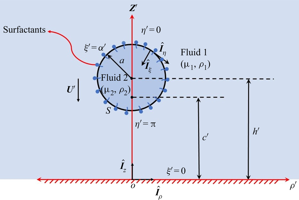
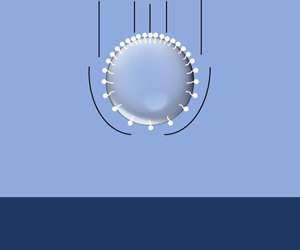
A schematic representation of the system under consideration has been depicted in figure 1, where a drop of radius  $a$ settling towards a solid wall is considered. The distance of the centre of drop from the wall is
 $h'(t')$ (dimensional variables, except the properties are denoted with a ‘prime’), a function of time. The surrounding fluid (fluid-1) has density
 $\rho _1$ and viscosity
 $\mu _1$, whereas the droplet fluid (fluid-2) has density
 $\rho _2$ and viscosity
 $\mu _2$. The surface tension between the two fluids is
 $\gamma '$ and it is assumed that fluid-2 is slightly heavier than fluid-1 so that the drop settles with velocity
 $U'(t')$ downwards. A bispherical coordinate system
 $(\xi ', \eta ', \phi )$ (Brenner Reference Brenner1961) is used to describe the fluid motion. The origin
 $O$, of this coordinate system is located at the intersection of drop axis and the wall, at
 $z' = 0$. More details regarding the bispherical coordinates have been given in § 4. Like most other multiphase systems, here also we account for the presence of impurities, which are considered to be largely insoluble in the bulk and get adsorbed at the interface as surfactants (Stone & Leal Reference Stone and Leal1990; Pal Reference Pal1992; Danov et al. Reference Danov, Vlahovska, Horozov, Dushkin, Kralchevsky, Mehreteab and Broze1996; Mandal et al. Reference Mandal, Ghosh and Chakraborty2016). The concentration of these surfactants is denoted as
 $\varGamma '$, which mainly alters the interfacial tension, as discussed later.
Schematic of a drop of radius  $a$ bounded by a wall at
 $z' = 0$, falling with velocity
 $\boldsymbol {U}'$ in a medium with density
 $\rho _1$ and viscosity
 $\mu _1$ (gravity points downwards). The drop has density
 $\rho _2$ and viscosity
 $\mu _2$. The interface between the two fluids contains surfactants (concentration
 $\varGamma '$), which may accumulate there because of adsorption from the bulk. The surface tension of the pure drop is
 $\gamma '_s$. In a bispherical coordinate system (
 $\xi ', \eta ', \phi$), the drop interface is located at
 $\xi ' = \alpha '(t')$. A reference cylindrical coordinate system (
 $z',\rho ',\phi$), with its origin on the wall has also been shown in the schematic.

Before delving deep into the quantitative details of fluid motion, it is important to outline the major assumptions undertaken herein. First and foremost, we assume the flow to be viscosity dominated ( $Re \ll 1$,
 $Re$ is the Reynolds number) and inertial effects will be neglected altogether. Second, although ideally the problem of a settling drop is inherently unsteady, for slow and viscous motion of the fluids, the flow may be assumed to be quasi-steady (Brenner Reference Brenner1961), without sacrificing the essential physics. Such an assumption has been widely used previously (Brenner Reference Brenner1961; Wacholder & Weihs Reference Wacholder and Weihs1972; Rushton & Davies Reference Rushton and Davies1973) and mandates that the motion in and around the drop solely depends on its instantaneous position. Further insights into the quasi-steady assumption are given in § 4.2 and the supplementary material available at https://doi.org/10.1017/jfm.2020.1101 (see § S1 therein) . At the same time, slow motion in the fluid also entails a low capillary number (
 $Ca = \mu _1 U_c/\gamma '_s$,
 $U_c$ - characteristic velocity, defined later), which leads to small deformation and hence the droplet may be assumed to remain approximately spherical (Stone & Leal Reference Stone and Leal1990; Leal Reference Leal2007; Hanna & Vlahovska Reference Hanna and Vlahovska2010).
As mentioned earlier, the impurities (or, surfactants) present in the system are assumed to be insoluble in bulk fluid (Stone & Leal Reference Stone and Leal1990; Cuenot et al. Reference Cuenot, Magnaudet and Spennato1997; Hanna & Vlahovska Reference Hanna and Vlahovska2010; Mandal et al. Reference Mandal, Ghosh and Chakraborty2016; Poddar et al. Reference Poddar, Mandal, Bandopadhyay and Chakraborty2018). To justify such an assumption, we first note that although impurities might have limited solubility in the bulk, their primary influence on the droplet motion comes because of their presence at the interface. In particular, interfacial concentration of the surfactants becomes a dominant factor, when the bulk diffusion and adsorption processes are slower as compared with interfacial convection (Leal Reference Leal2007). In fact, transport of the surfactant in the bulk may be neglected as a reasonably good first approximation, when the surfactant Biot number (defined as (Leal Reference Leal2007)  $Bi = {\alpha a}/{U_c}$,
 $\alpha$ is the surfactant desorption rate) is less than unity (Leal Reference Leal2007). Then, only the interfacial transport of the surfactant becomes important, which dictates the influence of these impurities on the droplet motion (Stone & Leal Reference Stone and Leal1990; Hanna & Vlahovska Reference Hanna and Vlahovska2010; Mandal et al. Reference Mandal, Ghosh and Chakraborty2016; Poddar et al. Reference Poddar, Mandal, Bandopadhyay and Chakraborty2018). We shall consider this so-called ‘insoluble limit’ in the present study. For further details on surface adsorption kinetics, one may refer to Leal (Reference Leal2007). It is also relevant to note that several previous studies (Stone & Leal Reference Stone and Leal1990; Li & Pozrikidis Reference Li and Pozrikidis1997; Hanna & Vlahovska Reference Hanna and Vlahovska2010; Mandal et al. Reference Mandal, Ghosh and Chakraborty2016) have also considered the insoluble surfactant limit, wherein only the interfacial transport was taken into account. We assume that the surfactant changes the interfacial surface tension (
 $\gamma '$) as (Stone & Leal Reference Stone and Leal1990; Poddar et al. Reference Poddar, Mandal, Bandopadhyay and Chakraborty2018)
 $\gamma ' = \gamma '_{s} - \varGamma 'RT$, where
 $\gamma '$ is the actual surface tension,
 $\gamma '_s$ is the interfacial tension for a clean interface,
 $T$ is absolute temperature and
 $R$ is the universal gas constant. The above relation suggests that the surface tension varies linearly with surfactant concentration, which remains valid only for dilute solutions, where
 $\varGamma '$ is smaller than a critical value (Leal Reference Leal2007).
3. Governing equations and boundary conditions in the small deformation limit
We consider a stationary frame of reference, attached to the wall. The velocity field and pressure in both the fluids obey the Stokes flow and continuity equations for quasi-steady flow (Brenner Reference Brenner1961)
 \begin{equation} \mu_k \nabla^{\prime 2} \boldsymbol{u}'_{k} - \boldsymbol{\nabla} p'_{k} = 0; \quad \boldsymbol{\nabla}'\boldsymbol{\cdot}\boldsymbol{u}'_{k} = 0,\quad k = 1, 2. \end{equation}
The steady-state interfacial surfactant transport equation, in the insoluble surfactant limit, is given as (Mandal et al. Reference Mandal, Ghosh and Chakraborty2016)
 \begin{equation} \boldsymbol{\nabla}'_{s}\boldsymbol{\cdot}(\boldsymbol{u}'_{s} \varGamma') = D \nabla^{\prime 2}_{s} \varGamma^{\prime}. \end{equation}
Here,  $\boldsymbol {\nabla }'_{s} = \boldsymbol {\nabla }' - \hat {\boldsymbol {n}}(\hat {\boldsymbol {n}}\boldsymbol {\cdot }\boldsymbol {\nabla }')$ (Leal Reference Leal2007) is the surface gradient operator,
 $\hat {\boldsymbol {n}}$ is the unit outward normal to the interface and
 $\boldsymbol {u}'_{s}$ is the fluid velocity on the drop interface relative to its centre. Notice that (3.2) is only satisfied at the fluid–fluid interface. Equations (3.1) are subjected to following far-field boundary conditions (Sadhal & Oguz Reference Sadhal and Oguz1985):
 \begin{equation} \boldsymbol{u}'_{1}\longrightarrow 0 \quad \rm{as,} \quad (\rho^{\prime 2}+z^{\prime 2})^{{1}/{2}}\longrightarrow \infty. \end{equation}
The velocity inside the drop remains bounded and thus  $|\boldsymbol {u}'_{2}| < \infty$ also needs to be satisfied. At the droplet interface (
 $\xi '=\alpha '(t')$, defined in § 4), the following boundary conditions are satisfied (Leal Reference Leal2007):
 \begin{gather} (\boldsymbol{u}'_{1} - \boldsymbol{U}')\boldsymbol{\cdot} \hat{\boldsymbol{n}} = 0,\quad \boldsymbol{u}'_{2}\boldsymbol{\cdot} \hat{\boldsymbol{n}} = 0, \end{gather}
 \begin{gather}(\boldsymbol\delta-\hat{\boldsymbol{n}}\hat{\boldsymbol{n}})\boldsymbol{\cdot}(\boldsymbol{u}'_{1} - \boldsymbol{U}') = (\boldsymbol\delta-\hat{\boldsymbol{n}}\hat{\boldsymbol{n}})\boldsymbol{\cdot}\boldsymbol{u}'_{2}, \end{gather}
 \begin{gather}(\boldsymbol\delta-\hat{\boldsymbol{n}}\hat{\boldsymbol{n}})\boldsymbol{\cdot}[(\boldsymbol{\tau}'_{1} - \boldsymbol{\tau}'_{2})\boldsymbol{\cdot}\hat{\boldsymbol{n}}] + (\boldsymbol\delta-\hat{\boldsymbol{n}}\hat{\boldsymbol{n}})\boldsymbol{\cdot}(\boldsymbol{\nabla}'_{s} \gamma') = 0, \end{gather}
 \begin{gather}p'_2-p'_1+[(\boldsymbol{\tau}'_{1} - \boldsymbol{\tau}'_{2})\boldsymbol{\cdot}\hat{\boldsymbol{n}}]\boldsymbol{\cdot}\hat{\boldsymbol{n}} = \gamma'(\boldsymbol{\nabla}'\boldsymbol{\cdot}\hat{\boldsymbol{n}}). \end{gather}
In (3.4c) and (3.4d), the stress tensor in the  $k$-th fluid is given as
 $\boldsymbol {\tau }'_{k} = \mu _k[\boldsymbol {\nabla }' \boldsymbol {u}'_{k} + (\boldsymbol {\nabla }' \boldsymbol {u}'_{k})^{T}]$;
 $\boldsymbol {u}'_1$ is the total velocity outside the drop with respect to the wall and
 $\boldsymbol {u}'_2$ is the relative velocity inside the drop with respect to its centre. Finally, on the wall the velocity field satisfies the no-penetration and no-slip boundary conditions, given by (Brenner Reference Brenner1961)
 \begin{equation} \boldsymbol{u}'_{1}\boldsymbol{\cdot}\hat{\boldsymbol{i}}_z = 0, \quad \boldsymbol{u}'_{1}\boldsymbol{\cdot}\hat{\boldsymbol{i}}_{\rho} = 0. \end{equation}
Because of fluid motion, it is evident from (3.2) that the surfactant concentration  $\varGamma '$ would differ from its equilibrium value, say,
 $\varGamma '_{eq}$, as follows (Stone & Leal Reference Stone and Leal1990; Leal Reference Leal2007; Mandal et al. Reference Mandal, Ghosh and Chakraborty2016):
 $\varGamma ' = \varGamma '_{eq}+\varGamma '_1$, where
 $\varGamma '_1$ quantifies the deviation. Therefore, the correct choice of equilibrium surface tension is,
 $\gamma '_{eq} = \gamma '_s-\varGamma '_{eq}RT$ and then surface tension may be represented in terms of
 $\varGamma '_1$ as follows (Stone & Leal Reference Stone and Leal1990; Pak et al. Reference Pak, Feng and Stone2014; Mandal et al. Reference Mandal, Ghosh and Chakraborty2016):
 $\gamma ' = \gamma '_{eq} - \varGamma '_1RT$.
We non-dimensionalize the above governing equations and boundary conditions as follows. For any variable, say  $\chi '$ (this might represent variables such as,
 $\boldsymbol {u}', p'$, etc.), its dimensionless version is expressed as
 $\chi = \chi '/\chi _c$, where
 $\chi _c$ is the characteristic scale for the said variable. Notice that the dimensionless variables are represented without any ‘prime’ symbol. The following characteristic scales are chosen for the different variables:
 $u_c = U_c = ({4}/{3})({{\rm \pi} a^2g}/{\mu _1}) (\rho _2-\rho _1), l_c = a, p_c = \tau _c = {\mu _kU_c}/{a},\ \textrm {for}\ k=1,2, \ \gamma _c = \gamma '_{eq}$ and
 $\varGamma _c = \varGamma '_{eq}$. We further define the ratio of viscosities of two fluids as
 $\lambda = {\mu _2}/{\mu _1}$. Upon enforcing the above characteristic scales in our governing equations and boundary conditions ((3.1)–(3.5a,b)), we deduce the following:
 \begin{gather} \nabla^{2} \boldsymbol{u}_{k} - \boldsymbol{\nabla} p_{k} = 0, \quad \boldsymbol{\nabla}\boldsymbol{\cdot}\boldsymbol{u}_{k} = 0, \quad \textrm{for}\ k = 1,2, \end{gather}
 \begin{gather}Pe \boldsymbol{\nabla}_{s}\boldsymbol{\cdot}(\boldsymbol{u}_{s} \varGamma) = \nabla^{2}_{s} \varGamma. \end{gather}
These are subjected to following boundary conditions at the interface S:
 \begin{gather} (\boldsymbol{u}_{1} - \boldsymbol{U})\boldsymbol{\cdot} \hat{\boldsymbol{n}} = 0, \quad \boldsymbol{u}_{2}\boldsymbol{\cdot} \hat{\boldsymbol{n}} = 0, \end{gather}
 \begin{gather}(\boldsymbol\delta-\hat{\boldsymbol{n}}\hat{\boldsymbol{n}})\boldsymbol{\cdot}(\boldsymbol{u}_{1} - \boldsymbol{U}) = (\boldsymbol\delta-\hat{\boldsymbol{n}}\hat{\boldsymbol{n}})\boldsymbol{\cdot}\boldsymbol{u}_{2}, \end{gather}
 \begin{gather}(\boldsymbol\delta-\hat{\boldsymbol{n}}\hat{\boldsymbol{n}})\boldsymbol{\cdot}[(\boldsymbol{\tau}_{1} - \lambda\boldsymbol{\tau}_{2})\boldsymbol{\cdot}\hat{\boldsymbol{n}}] + \frac{1}{Ca_s}(\boldsymbol\delta-\hat{\boldsymbol{n}}\hat{\boldsymbol{n}})\boldsymbol{\cdot}(\boldsymbol{\nabla}_{s} \gamma) = 0, \end{gather}
 \begin{gather}\lambda p_{2} - p_{1} + [(\boldsymbol{\tau}_{1} - \lambda\boldsymbol{\tau}_{2})\hat{\boldsymbol{n}}]\boldsymbol{\cdot}\hat{\boldsymbol{n}} = \frac{\gamma}{Ca_s}(\boldsymbol{\nabla}\boldsymbol{\cdot}\hat{\boldsymbol{n}}). \end{gather}
In (3.8c) and (3.8d),  $Ca_s = {\mu _1 U_c}/{\gamma '_{eq}}$, is an appropriate choice for the capillary number (Stone & Leal Reference Stone and Leal1990; Mandal et al. Reference Mandal, Ghosh and Chakraborty2016; Poddar et al. Reference Poddar, Mandal, Bandopadhyay and Chakraborty2018), and in (3.7),
 $Pe = U_c a/D$ is the surfactant Péclet number (Stone & Leal Reference Stone and Leal1990; Mandal et al. Reference Mandal, Ghosh and Chakraborty2016). The resulting surface tension is now defined as
 $\gamma = 1-({\beta }/({1-\beta }))\varGamma _1$, where
 $\beta = {RT\varGamma '_{eq}}/{\gamma '_s}$ defines the sensitivity of the surface tension to the changes in the surfactant concentration (Stone & Leal Reference Stone and Leal1990) and is related to the Marangoni number (
 $Ma = {RT\varGamma '_{eq}}/{\mu _1U_c}$) as
 $\beta = Ca\cdot Ma$ (Pak et al. Reference Pak, Feng and Stone2014). The value of
 $\beta$ is restricted between 0 and 1. The Reynolds number may be defined as
 $Re = \rho _1 U_c a/\mu _1$. Further notice that the total surfactant concentration now reads:
 $\varGamma = 1+\varGamma _1$ (Mandal et al. Reference Mandal, Ghosh and Chakraborty2016). Finally, the boundary conditions on the wall at
 $z = 0$ become
 \begin{equation} \boldsymbol{u}_{1}\boldsymbol{\cdot}\hat{\boldsymbol{i}}_z = 0, \quad \boldsymbol{u}_{1}\boldsymbol{\cdot}\hat{\boldsymbol{i}}_{\rho} = 0. \end{equation}
The far-field condition remains the same, as given in (3.3). As mentioned in § 2, here we shall consider the small deformation limit, which entails  $Ca_s\ll 1$ (also
 $Ca \ll 1$) (Stone & Leal Reference Stone and Leal1990; Ha & Yang Reference Ha and Yang1995; Leal Reference Leal2007; Hanna & Vlahovska Reference Hanna and Vlahovska2010; Mandal et al. Reference Mandal, Ghosh and Chakraborty2016; Poddar et al. Reference Poddar, Mandal, Bandopadhyay and Chakraborty2018). At this juncture, it is important to note that because the flow here is viscosity dominated,
 $Ca$ (defined as the ratio of viscous to surface tension force) governs the interfacial stress balance. On the other hand, for inertia dominated flows, Weber number,
 $We = ({\rho _1 U_c^2 a})/{\gamma '_s}$ will govern the balance between the interfacial stresses (Chandra & Avedisian Reference Chandra and Avedisian1991). This can be better understood from noting that
 $We = Ca.Re$ and because both
 $Re\ll 1$ and
 $Ca< O(1)$ here,
 $We\ll 1$ in the present scenario. We shall further assume,
 $Pe\sim O(Ca_s)$, i.e.
 $Pe = kCa_s$, where
 $k$ is an
 $O(1)$ constant, a paradigm previously considered by several studies (Stone & Leal Reference Stone and Leal1990; Ha & Yang Reference Ha and Yang1995). Physically, this indicates that the effect of surfactant advection is weak (Pak et al. Reference Pak, Feng and Stone2014) and thus the surfactant concentration deviates by a small amount from its equilibrium value. A detailed discussion on the validity of this assumption may be found in the work of Mandal et al. (Reference Mandal, Ghosh and Chakraborty2016). We would emphasize that several other studies (Hanna & Vlahovska Reference Hanna and Vlahovska2010; Poddar et al. Reference Poddar, Mandal, Bandopadhyay and Chakraborty2018) have also ventured into the small deformation and weak advection paradigm, when accounting for surfactant transport, wherein formulation equivalent to
 $Pe = kCa_s$ has been employed. The above assumptions enable us to write asymptotic expansions for all the flow variables in terms of
 $Ca_s$ (Mandal et al. Reference Mandal, Ghosh and Chakraborty2016). Therefore, any variable, say
 $\chi$ (represent variables such as
 $\boldsymbol {u}, p,\ldots$ etc.), may be expressed as follows:
 \begin{equation} \chi = \chi^{(0)}+ Ca_s\chi^{(1)}+\cdots. \end{equation}
Noting that  $Pe = kCa_s$, the deviation in the surfactant concentration (
 $\varGamma _1$) may be expanded as (Pak et al. Reference Pak, Feng and Stone2014; Mandal et al. Reference Mandal, Ghosh and Chakraborty2016)
 \begin{equation} \varGamma_1 = kCa_s\varGamma^{(1)}_1+\cdots. \end{equation}
Notice that the expansion for  $\varGamma _1$ starts at
 $O(Ca_s)$, because for
 $Ca_s= 0$,
 $Pe = 0$, which indicates absence of any interfacial advection and hence the surfactant concentration will be equal to the equilibrium concentration everywhere. Because of the stresses acting on the drop interface, it will deform from its initial spherical shape. In the bispherical coordinate (
 $\xi , \eta , \phi$), the surface of a spherical drop is expressed as
 $\xi = \alpha$, where
 $\alpha$ only depends on time (see § 4). Then the shape of the deformed drop is expressed as
 \begin{equation} F \equiv \xi - [\alpha + Ca_sf(\eta)+ \cdots] = 0. \end{equation}
In (3.12),  $f(\eta )$ is the net deformation at the interface, which here is only a function of the polar angle
 $\eta$ (see figure 1), because of the inherent axisymmetry of the dynamics (Brenner Reference Brenner1961; Wacholder & Weihs Reference Wacholder and Weihs1972). The normal to the interface is given by
 \begin{equation} \hat{\boldsymbol{n}} = \hat{\boldsymbol{i}}_{\xi} - \hat{\boldsymbol{i}}_{\eta} Ca_s\frac{\textrm{d}f(\eta)}{\textrm{d}\eta}. \end{equation}
In the paradigm of small  $Ca_s$ (small deformation), to stick to an elegant semianalytical framework, we shall only consider the leading-order terms in the asymptotic expansions reported in (3.10), (3.11), and in the process we shall discard the ‘
 ${(0)}$’ superscript from all the variables to make the notation simpler. A justification for such consideration has been provided while discussing the results in § 5. The resulting leading-order equations take the following form (Mandal et al. Reference Mandal, Ghosh and Chakraborty2016):
 \begin{gather} \nabla^{2} \boldsymbol{u}_{k} - \boldsymbol{\nabla} p_{k} = 0, \quad \boldsymbol{\nabla}\boldsymbol{\cdot}\boldsymbol{u}_{k} = 0, \quad \text{for}\ k = 1,2, \end{gather}
 \begin{gather}\boldsymbol{\nabla}_{s}\boldsymbol{\cdot}\boldsymbol{u}_{s} = \nabla^{2}_{s} \varGamma^{(1)}_1. \end{gather}
These are subjected to following boundary conditions at the interface  $S$:
 \begin{gather} (\boldsymbol{u}_{1} - \boldsymbol{U})\boldsymbol{\cdot} \hat{\boldsymbol{n}} = 0, \quad \boldsymbol{u}_{2}\boldsymbol{\cdot} \hat{\boldsymbol{n}} = 0, \end{gather}
 \begin{gather}(\boldsymbol\delta-\hat{\boldsymbol{n}}\hat{\boldsymbol{n}})\boldsymbol{\cdot}(\boldsymbol{u}_{1} - \boldsymbol{U}) = (\boldsymbol\delta-\hat{\boldsymbol{n}}\hat{\boldsymbol{n}})\boldsymbol{\cdot}\boldsymbol{u}_{2}, \end{gather}
 \begin{gather}(\boldsymbol\delta-\hat{\boldsymbol{n}}\hat{\boldsymbol{n}})\boldsymbol{\cdot}[(\boldsymbol{\tau}_{1} - \lambda\boldsymbol{\tau}_{2})\boldsymbol{\cdot}\hat{\boldsymbol{n}}] = \omega\boldsymbol{\nabla}_{s} \varGamma^{(1)}_1 \boldsymbol{\cdot}(\boldsymbol\delta-\hat{\boldsymbol{n}}\hat{\boldsymbol{n}}), \end{gather}
 \begin{gather}\lambda p_{2} - p_{1} + [(\boldsymbol{\tau}_{1} - \lambda\boldsymbol{\tau}_{2})\boldsymbol{\cdot}\hat{\boldsymbol{n}}]\boldsymbol{\cdot}\hat{\boldsymbol{n}} = \frac{2}{Ca_s}- 2f-\nabla^2_{s}f - 2\omega\varGamma^{(1)}_1. \end{gather}
In (3.16c) and (3.16d), we define  $\omega = {\beta k}/{(1-\beta )}$ (Mandal et al. Reference Mandal, Ghosh and Chakraborty2016). The boundary conditions on the wall (
 $z=0$) remain the same as discussed in (3.9a,b) and hence are not repeated here.
Equations (3.14) and (3.15), subjected to the boundary conditions (3.16a)–(3.16c) completely describe the flow in and around the drop at a particular distance,  $h$, from the wall. We write semianalytical solutions to these equations in the next section, which are subsequently used to determine the droplet velocity as a function of its distance from the wall, by doing an overall force balance on the drop. This, in turn, will dictate how the distance
 $h$ varies with time, as the drop settles towards the wall. In this context, it should be noted that for
 $Re\sim O(1)$ or larger, i.e. when inertial terms become important, it is not possible to write exact analytical/semianalytical solutions.
4. Approximate analytical solutions
Considering the nature of the problem, we describe the fluid motion using bispherical coordinates ( $\xi , \eta , \phi$). The droplet and the wall can be simultaneously represented in this coordinate system, as shown in figure 1. The surface of the undeformed drop (spherical) is expressed as
 $\xi = \alpha$ and the surface of the wall is then represented as
 $\xi = 0$. Note that (see figure 1)
 $\hat {\boldsymbol {i}}_{\xi }$ and
 $\hat {\boldsymbol {i}}_{\eta }$ denote the normal and tangential unit vectors on the drop surface and the vector
 $\hat {\boldsymbol {i}}_{\xi }$ is directed inwards. A reference cylindrical coordinate system (
 $z,\rho ,\phi$) has also been placed with its origin on the wall and along the same vertical line as that of the drop's motion. These two coordinates may be related by using the conformal transformation (Happel & Brenner Reference Happel and Brenner2012)
 $z+i\rho = ic \cot (({\eta + i\xi })/{2})$, where
 $c$ is a positive constant that depends on
 $h$ – the distance of the drop centre from the wall. It may then be shown that the above conformal mapping simply leads to
 \begin{equation} \rho = \frac{c \sin \eta}{\cosh \xi - \cos \eta}; \quad z = \frac{c \sinh \xi}{\cosh \xi - \cos \eta}; \quad \phi = \phi. \end{equation}
The (4.1a–c) represent non-dimensional quantities, for which the characteristic scales have been given in § 3. The scale factors for bipolar coordinate system are expressed as (Happel & Brenner Reference Happel and Brenner2012)
 \begin{equation} h_1 = h_2 = \frac{\cosh \xi - \cos \eta}{c}, \quad h_3 = \frac{\cosh \xi - \cos \eta}{c \sin \eta}.\nonumber \end{equation}
From (4.1a–c), we deduce the following relations:  $c = \sinh \alpha , h = \cosh \alpha$ (Brenner Reference Brenner1961; Happel & Brenner Reference Happel and Brenner2012). It is important to realize that both
 $\alpha$ and hence
 $c$ depend only on
 $h(t)$, i.e. the distance of the drop centre from the wall. As the drop settles,
 $h(t)$ changes with time and so does
 $\alpha$ and
 $c$, which emerges from the inherent unsteadiness of the problem. However, the quasi-steady assumption would indicate that the flow dynamics may be evaluated at any instant by solving (3.14) and (3.15), subjected to the boundary conditions (3.16a)–(3.16c) for the particular
 $c$ and
 $\alpha$ at that instant, which in turn would depend on
 $h(t)$.
4.1. Solution for the flow field
In view of the intrinsic axisymmetry of the problem, we may solve (3.14) and (3.15) subject to (3.16a)–(3.16c) by using a stream function ( $\varPsi _k$ in fluid
 $k$,
 $k = 1,2$) (Leal Reference Leal2007). The velocity components in the bipolar coordinate (
 $u_{\xi }$ and
 $u_{\eta }$) are related to the stream function as follows (Wacholder & Weihs Reference Wacholder and Weihs1972; Mandal et al. Reference Mandal, Ghosh and Chakraborty2016):
 \begin{equation} u^{(k)}_\xi = \frac{(\cosh \xi - \cos \eta)^2}{c^2 \sin \eta} \frac{\partial\varPsi_k}{\partial\eta}; \quad u^{(k)}_\eta = -\frac{(\cosh \xi - \cos \eta)^2}{c^2 \sin \eta} \frac{\partial\varPsi_k}{\partial\xi}. \end{equation}
It may be shown that the stokes flow equation (i.e. (3.14)) may be expressed in terms of stream function as follows (Brenner Reference Brenner1961):  $\mathcal {E}^4\varPsi = 0$, where
 $\mathcal {E}^2 = {\partial ^2}/{\partial z^2} + \rho ({\partial }/{\partial \rho }) ( ({1}/{\rho })({\partial }/{\partial \rho }))$. It can also be shown that the stream function
 $\varPsi$ may be expressed in the following general form (Stimson & Jeffery Reference Stimson and Jeffery1926; Brenner Reference Brenner1961):
 \begin{equation} \varPsi_k = (\cosh \xi-\zeta)^{-{3}/{2}} \sum_{n=0}^{\infty} W^{(k)}_n(\xi) C^{-{1}/{2}}_{n+1}(\zeta). \end{equation}
In (4.3),  $\zeta = \cos \eta$,
 $C^{-{1}/{2}}_{n+1}(\zeta )$ is Gegenbauer polynomial of order
 $n+1$ and degree
 $-{1}/{2}$. The expressions for
 $W^{(k)}_n(\xi )$ (k = 1,2) are given by (Wacholder & Weihs Reference Wacholder and Weihs1972)
 \begin{gather} W^{(1)}_n(\xi) = A^{*}_n\cosh\left(n-\tfrac{1}{2}\right)\xi + B^{*}_n\sinh\left(n-\tfrac{1}{2}\right)\xi + C^{*}_n\cosh\left(n+\tfrac{3}{2}\right)\xi\nonumber\\ + D^{*}_n\sinh\left(n+\tfrac{3}{2}\right)\xi, \end{gather}
 \begin{gather}W^{(2)}_n(\xi) = E^{*}_n \exp\left({-\left(n-\tfrac{1}{2}\right)\xi}\right) + F^{*}_n \exp\left({-\left(n+\tfrac{3}{2}\right)\xi}\right). \end{gather}
In (4.4b), the positive exponential powers will not be present, to ensure that the velocity field remains bounded inside the drop (Mandal et al. Reference Mandal, Ghosh and Chakraborty2016). Boundary conditions (i.e. conditions (3.16a)–(3.16d)) on the drop surface ( $\xi = \alpha$) may be written as follows (in the bipolar coordinate Mandal et al. (Reference Mandal, Ghosh and Chakraborty2016)):
 \begin{gather} u^{(1)}_\xi = \boldsymbol{U}\boldsymbol{\cdot}\hat{\boldsymbol{i}}_{\xi}, \quad u^{(2)}_\xi =0, \end{gather}
 \begin{gather}u^{(1)}_\eta = \boldsymbol{U}\boldsymbol{\cdot}\hat{\boldsymbol{i}}_{\eta} + u^{(2)}_\eta, \end{gather}
 \begin{gather}\tau^{(1)}_{\xi\eta} - \lambda\tau^{(2)}_{\xi\eta} = -\omega h_1\frac{\partial \varGamma^{(1)}_1}{\partial \eta}, \end{gather}
 \begin{gather}\lambda p_{2} - p_{1} + \tau^{(1)}_{\xi\xi} - \lambda\tau^{(2)}_{\xi\xi} = - \frac{\gamma}{Ca_s}(\boldsymbol{\nabla}\boldsymbol{\cdot}\hat{\boldsymbol{n}}). \end{gather}
In (4.5c), the tangential stress components in the  $k$-th fluid (i.e.
 $\tau ^{(k)}_{\xi \eta }$) may be written as (Wacholder & Weihs Reference Wacholder and Weihs1972; Mandal et al. Reference Mandal, Ghosh and Chakraborty2016)
 \begin{equation} \tau^{(k)}_{\xi\eta} = h_2\left[\frac{\partial u^{(k)}_\eta}{\partial \xi} - h_1 u^{(k)}_\xi\frac{\partial}{\partial \eta}\left(\frac{1}{h_2}\right)\right] + h_1\left[\frac{\partial u^{(k)}_\xi}{\partial \eta} - h_2 u^{(k)}_\eta\frac{\partial}{\partial \xi}\left(\frac{1}{h_1}\right)\right]. \end{equation}
The conditions at the wall and the far field, both represented by  $\xi = 0$, boil down to the following (Brenner Reference Brenner1961; Wacholder & Weihs Reference Wacholder and Weihs1972):
 \begin{equation} u^{(1)}_\xi = u^{(1)}_\eta = 0\quad \text{at}\ \xi = 0. \end{equation}
The surfactant transport (3.15) may be simplified by noting that in bipolar coordinate, the surface gradient operator is defined as (Happel & Brenner Reference Happel and Brenner2012)  $\boldsymbol {\nabla }_s = \hat {\boldsymbol {i}_\eta }h_1({\partial }/{\partial \eta }) + \hat {\boldsymbol {i}}_{\phi } h_3({\partial }/{\partial \phi })$ and the surface divergence of any vector
 $\boldsymbol {V}$ (
 $\boldsymbol {V} = V_\eta \hat {\boldsymbol {i}}_{\eta } + V_\xi \hat {\boldsymbol {i}}_{\xi } + V_\phi \hat {\boldsymbol {i}}_{\phi }$), reads (for axisymmetric cases)
 \begin{equation} \boldsymbol{\nabla}_s\boldsymbol{\cdot}\boldsymbol{V} = h_1h_2h_3\left[\frac{\partial}{\partial \eta}\left(\frac{V_\eta}{h_2h_3}\right) + \frac{\partial}{\partial \xi}\left(\frac{V_\xi}{h_1h_3}\right)\right] - h_1h_2V_\eta\frac{\partial}{\partial \eta}\left(\frac{1}{h_2}\right) - h_2\frac{\partial V_\xi}{\partial \xi}. \end{equation}
In view of the solutions given in (4.4a) and (4.4b), the tangential stress balance condition (4.5c), in combination with (4.6), we infer that the surfactant concentration must have the following form (Mandal et al. Reference Mandal, Ghosh and Chakraborty2016):
 \begin{equation} \frac{\partial\varGamma^{(1)}_1}{\partial \zeta} = \frac{(\cosh\xi - \zeta)^{-{1}/{2}}}{c^2(1-\zeta^2)}\sum_{n=0}^{\infty} Z^{*}_nC^{-{1}/{2}}_{n+1}(\zeta), \end{equation}
where  $Z^{*}_n$ (
 $n\geq 0$) are constants yet to be determined. The surfactant concentration can be found out by integrating the above equation. To ensure that the total surfactant mass is conserved,
 $\varGamma (\eta )$ (
 $= 1 + kCa_s\varGamma ^{(1)}_1$) would also satisfy the following condition (Poddar et al. Reference Poddar, Mandal, Bandopadhyay and Chakraborty2018):
 $\int _{A}\varGamma dA = 2$, where the integration is carried out over the drop surface.
Noting that the stream function and the surfactant concentration must be a linear function of the droplet velocity  $U$ (non-dimensionalized by
 $U_c$, see § 3), we infer that the unknown constants in (4.4a), (4.4b) and (4.9) (i.e. the constants
 $A^{*}_n,B^{*}_n,C^{*}_n,\ldots$, etc.) must have the following form (Mandal et al. Reference Mandal, Ghosh and Chakraborty2016):
 \begin{gather} A^{*}_n = A_n(\lambda,\omega)Uc^2, \quad B^{*}_n = B_n(\lambda,\omega)Uc^2, \quad C^{*}_n = C_n(\lambda,\omega)Uc^2, \quad D^{*}_n = D_n(\lambda,\omega)Uc^2,\nonumber\\ E^{*}_n = E_n(\lambda,\omega)Uc^2, \quad F^{*}_n = F_n(\lambda,\omega)Uc^2, \quad Z^{*}_n = Z_n(\lambda,\omega)Uc^2. \end{gather}
Upon inserting the expressions (4.4a), (4.4b) and (4.9) into the boundary conditions in (4.5a)–(4.5c) and taking into account (4.2a,b), (4.3) and (4.10a–g), we may deduce a set of coupled linear algebraic equations to determine the constants,  $A_n,B_n,C_n,D_n,E_n,F_n$ and
 $Z_n$ for all
 $n\geq 0$. The said linear system of equations, as well as more detailed treatment of the boundary conditions, have been included in appendix A. It has been previously shown (Wacholder & Weihs Reference Wacholder and Weihs1972) that in the absence of any surfactant (
 $Z_n = 0,\forall n$), for each
 $n$ one gets a set of six independent algebraic equations, which may be solved analytically to deduce the constants
 $A_n$ to
 $F_n$. However, in the presence of surface impurities, as considered herein, the equations for a given
 $n$ (say,
 $n = 3$) would contain the coefficients corresponding to all other values of
 $n$. This indicates that the individual coefficients must be computed by solving an infinitely large system of coupled linear algebraic equations, which results in a loss of analytical tractability. In an effort to compute the solutions, we thus truncate the series for
 $\varPsi _k$ and
 $\varGamma _1$ after
 $N = 15$ terms (Mandal et al. Reference Mandal, Ghosh and Chakraborty2016), which yields a system of 105 coupled equations with 105 unknowns (seven unknowns for each
 $n$). We solve these equations numerically. We also observe that choosing the first
 $N = 15$ terms in the series solution (4.3) is sufficient for convergence, even close to the wall. For further information, see § S2 of the supplementary material.
4.2. The settling velocity of the drop
The droplet velocity is computed by considering the balance between the hydrodynamic drag exerted by the fluid and the net gravitational force acting on the drop. The hydrodynamic drag (dimensional form) may be expressed as (Stimson & Jeffery Reference Stimson and Jeffery1926; Brenner Reference Brenner1961; Mandal et al. Reference Mandal, Ghosh and Chakraborty2016)
 \begin{equation} F'_D = \mu_1aU_c\left[\frac{{\rm \pi}2\sqrt{2}}{c}\sum_{n=0}^{\infty} \left( A^{*}_n+B^{*}_n+C^{*}_n+D^{*}_n\right)\right]. \end{equation}
On the other hand, the net downwards gravitational force acting on the drop is given by  $F'_G = ({4}/{3}){\rm \pi} a^3g(\rho _2-\rho _1)$. Here,
 $g$ is the acceleration due to gravity. We now choose the characteristic force as
 $F_c = \mu _1 a U_c$. The simplest way to evaluate the velocity is to equate the instantaneous hydrodynamic drag to the weight of the drop; this yields
 \begin{equation} U = \frac{1}{{\rm \pi}2\sqrt{2}c\sum_{n=0}^{\infty}\left(A_n+B_n+C_n+D_n\right)}. \end{equation}
Notice that since the constants depend on  $h$, the drop velocity in (4.12) also depends strongly on
 $h$ and hence
 $t$. As a result, we can now determine
 $h(t)$, by simply integrating the equation,
 ${\textrm {d}h}/{\textrm {d}t} = -U(h;\lambda ,\omega )$, subject to some initial condition.
It is perhaps more accurate to solve for the velocity of the drop as well as its position, by writing the overall force balance for the entire drop, also taking into account its acceleration. As such, we may write  $({4}/{3}){\rm \pi} a^3\rho _2({\textrm {d}^2h'(t')}/{\textrm {d}t^{\prime 2}}) = F'_D - F'_G$, where
 $F'_D$ is given by (4.11). By choosing the characteristic time as
 $t_c = {a}/{U_c}$, taking
 $U$ to be positive when the motion is downward (see figure 1) and finally substituting
 $U = -({\textrm {d}h(t)}/{\textrm {d}t})$ in the aforementioned force balance equation, we can deduce the following equation, which directly determines
 $h(t)$:
 \begin{equation} \frac{\textrm{d}^2h(t)}{\textrm{d}t^2} = M\frac{\textrm{d}h(t)}{\textrm{d}t} + N. \end{equation}
In (4.13),  $M = -({2\sqrt {2}a^2c\mu _1{\rm \pi} }/{U_cG_1})[ \sum _{n=0}^{\infty }(A_n+B_n+C_n+D_n)], N = -({aG_2}/{U^2_c})$, where,
 $G_1 = ({4}/{3}){\rm \pi} a^3\rho _2$ and
 $G_2 = {g(\rho _2-\rho _1)}/{\rho _2}$. Equation (4.13) is solved using the Runge–Kutta method, subject to
 $h(t=0) = h_0$ (given later) and
 ${\textrm {d}h}/{\textrm {d}t}(t=0) = 0$. Notice that
 $M$ implicitly depends on
 $h$, through the constants
 $A_n$ to
 $D_n$. Here we would like to emphasize that when the drop is close to the wall,
 $\Delta h' \sim h'-a$ (or,
 $\Delta h \sim h-1$) (see § 5.3) is perhaps a more accurate choice of the length scale, because the flow within the thin film residing between the drop and wall now governs the hydrodynamic drag. Although,
 $\Delta h \ll 1$ in this regime, the drop's velocity also reduces considerably (discussed later in detail), which is why the characteristic time scale of the flow (
 $\sim \Delta h'/U_c$) still remains larger than the viscous time scale (
 $\sim \Delta h'^2/\nu$). This enables us to treat the flow as being quasi-steady, even when the drop is close to the wall. In this context it is important to note that, although added mass effects may become important when the drop/bubble accelerates rapidly (Kok Reference Kok1993; Ohl, Tijink & Prosperetti Reference Ohl, Tijink and Prosperetti2003), to be consistent with the quasi-steady assumption, we have not included these effects in (4.13) (Landau & Lifshitz Reference Landau and Lifshitz1959; Leal Reference Leal2007). Further details can be found in the supplementary material (see § S1 therein).
Finally, it should be noted that the minimum  $h$ that can be captured by our analysis depends on the limitations of the continuum approximation. For very small values of
 $\Delta h' \sim h'-a$ (
 $\sim O(10\ \text {nm})$), non-hydrodynamic effects such as the van der Waals forces (Leal Reference Leal2007; Hu & Sun Reference Hu and Sun2013) start playing important roles in governing the flow, which has not been accounted for in our work.
4.3. Evaluation of droplet deformation
The droplet deformation can be determined from the normal stress balance (4.5d). Although an unbounded settling drop does not deform even with surfactants (Leal Reference Leal2007; Poddar et al. Reference Poddar, Mandal, Bandopadhyay and Chakraborty2018), deformation nevertheless sets in when bounding walls are present. This deformation, however, is quite small, as we show later. The normal stress balance requires evaluation of pressure; this may be done using the momentum equations, as follows (Chervenivanova & Zapryanov Reference Chervenivanova and Zapryanov1985) (for  $k = 1, 2$):
 \begin{equation} \frac{\partial p_k}{\partial \xi} = -\frac{(\cosh\xi - \zeta)}{c}\frac{\partial(\mathcal{E}^2\varPsi_k)}{\partial \zeta}\quad \text{and}\quad \frac{\partial p_k}{\partial \zeta} = \frac{(\cosh\xi - \zeta)}{c(1-\zeta^2)}\frac{\partial(\mathcal{E}^2\varPsi_k)}{\partial \xi}, \end{equation}
 $\mathcal {E}^2\varPsi$ (for both fluids) in bipolar coordinates may be expressed as (Stimson & Jeffery Reference Stimson and Jeffery1926)
 \begin{gather} \mathcal{E}^2\varPsi_k = \frac{\sqrt{(\cosh\xi - \zeta)}}{c^2} \sum_{n=0}^{\infty}\left[C^{-{1}/{2}}_{n+1}(\zeta)\left\{\frac{\textrm{d}^2W^{(k)}_n}{\textrm{d}\xi^2} - \frac{2\sinh\xi}{(\cosh\xi - \zeta)}\frac{\textrm{d}W^{(k)}_n}{\textrm{d}\xi}\right.\right.\nonumber\\ \left.\left.+ \frac{3(\cosh\xi + 3\zeta)}{4(\cosh\xi - \zeta)}W^{(k)}_n\right\} + (1-\zeta^2)W^{(k)}_n \left\{\frac{\textrm{d}^2C^{-{1}/{2}}_{n+1}}{\textrm{d}\zeta^2} + \frac{2}{(\cosh\xi - \zeta)}\frac{\textrm{d}C^{-{1}/{2}}_{n+1}}{\textrm{d}\zeta}\right\}\right]. \end{gather}
Using the expressions (4.4a), (4.4b) and recurrence relations for the Gegenbauer polynomials, (4.15) may be simplified as follows (Chervenivanova & Zapryanov Reference Chervenivanova and Zapryanov1985), for the inner and the outer fluids:
 \begin{gather} \mathcal{E}^2\varPsi_1 = \frac{1}{c^2\sqrt{(\cosh\xi - \zeta)}} \sum_{n=0}^{\infty}\left[a_n\cosh\left(n+\frac{1}{2}\right)\xi + b_n\sinh\left(n+\frac{1}{2}\right)\xi\right]C^{-{1}/{2}}_{n+1}, \end{gather}
 \begin{gather}\mathcal{E}^2\varPsi_2 = \frac{1}{c^2\sqrt{(\cosh\xi - \zeta)}} \sum_{n=0}^{\infty}\left[e_n\exp\left({-\left(n+\frac{1}{2}\right)\xi}\right)\right]C^{-{1}/{2}}_{n+1}, \end{gather}
where,
 \begin{gather} a_n = -(2n-1)A^{*}_n + (2n+3)C^{*}_n + 2n A^{*}_{n+1} - 2(n+1)C^{*}_{n-1}, \end{gather}
 \begin{gather}b_n = -(2n-1)B^{*}_n + (2n+3)D^{*}_n + 2n B^{*}_{n+1} - 2(n+1)D^{*}_{n-1}, \end{gather}
 \begin{gather}e_n = -(2n-1)E^{*}_n + (2n+3)F^{*}_n + 2n E^{*}_{n+1} - 2(n+1)F^{*}_{n-1}. \end{gather}
Since pressure is harmonic ( $\nabla ^2p_k = 0$), it has the same form as the general solution to the Laplace equation in bipolar coordinates (Jeffery Reference Jeffery1912; Subramanian & Balasubramanian Reference Subramanian and Balasubramanian2001). By taking into account the hydrostatic pressure, measured from the droplet centre, the total pressure may now be expressed as (Chervenivanova & Zapryanov Reference Chervenivanova and Zapryanov1985)
 \begin{gather} p_1 = \frac{\sqrt{(\cosh\xi - \zeta)}}{c^3} \sum_{n=0}^{\infty} \left[\alpha^{(1)}_n\cosh\left\{\left(n+\frac{1}{2}\right)\xi\right\} + \beta^{(1)}_n\sinh\left\{\left(n+\frac{1}{2}\right)\xi\right\}\right] P_n(\zeta)\nonumber\\ - \frac{\rho_1 g a^2}{\mu_1 U_c}\frac{(\zeta \cosh\xi - 1)}{(\cosh\xi - \zeta)} + \varPi^{(1)}, \end{gather}
 \begin{gather}p_2 = \frac{\sqrt{(\cosh\xi - \zeta)}}{c^3} \sum_{n=1}^{\infty} \left[\alpha^{(2)}_n \exp\left({-\left(n+\frac{1}{2}\right)\xi}\right)\right] P_n(\zeta)\nonumber\\ - \frac{\rho_2 g a^2}{\mu_1 U_c}\frac{(\zeta \cosh\xi - 1)}{(\cosh\xi - \zeta)} + \varPi^{(2)}. \end{gather}
In (4.18a) and (4.18b),  $P_n(\zeta )$ is a Legendre polynomial of degree 1 and order
 $n$;
 $\varPi ^{(1)}$ and
 $\varPi ^{(2)}$ are constants, yet to be determined;
 $\alpha ^{(k)}_n$ and
 $\beta ^{(k)}_n$ are also constants that are related to the constants appearing in the stream function. Substituting (4.16) on the right-hand side of (4.14a,b), (4.18) on the left-hand side of the same and using (4.18) along with the recurrence relations for the Legendre polynomials, we get the following expressions for the constants in the expressions for pressure (Chervenivanova & Zapryanov Reference Chervenivanova and Zapryanov1985):
 \begin{gather} \alpha^{(1)}_n = \sum_{m=1}^{n-1}\frac{b_m}{m(m+1)} + \frac{b_n}{n} + \alpha_0\quad \text{and}\quad \beta^{(1)}_n = \sum_{m=1}^{n-1}\frac{a_m}{m(m+1)} + \frac{a_n}{n} + \beta_0 , \end{gather}
 \begin{gather}\alpha^{(2)}_n = - \left[\sum_{m=1}^{n-1}\frac{e_m}{m(m+1)} + \frac{e_n}{n}\right]. \end{gather}
The constants  $\alpha _0,\beta _0$ have to be computed by ensuring that the pressure approaches a constant value far away from the drop (i.e.
 $\xi = 0$). This constraint yields the following relations (Chervenivanova & Zapryanov Reference Chervenivanova and Zapryanov1985):
 \begin{gather} \alpha_0 = -\lim_{n\rightarrow\infty}\left[\sum_{m=1}^{n-1}\frac{b_m}{m(m+1)} + \frac{b_n}{n}\right]\quad \text{and}\quad \beta_0 = -\lim_{n\rightarrow\infty}\left[\sum_{m=1}^{n-1}\frac{a_m}{m(m+1)} + \frac{a_n}{n}\right]. \end{gather}
In (4.5d), the normal stresses ( $\tau ^{(k)}_{\xi \xi }$) are also required to evaluate the deformation. It may be shown that these stresses, when expressed using bipolar coordinates, take the following form (Chervenivanova & Zapryanov Reference Chervenivanova and Zapryanov1985; Happel & Brenner Reference Happel and Brenner2012):
 \begin{equation} \tau^{(k)}_{\xi\xi} = 2h_2\left[\frac{\partial u^{(k)}_\xi}{\partial \xi} + h_1 u^{(k)}_\eta\frac{\partial}{\partial \eta}\left(\frac{1}{h_2}\right)\right],\quad k = 1, 2. \end{equation}
The normal stress may be simplified using (4.2a,b) in combination with (4.3), (4.4a) and (4.4b). Finally, the curvature of the drop surface up to  $O(Ca_s)$ in (4.5d) in bipolar coordinates can be found from the surface normal (
 $\hat {\boldsymbol {n}}$) in (3.13) as (Chervenivanova & Zapryanov Reference Chervenivanova and Zapryanov1985)
 \begin{gather} \boldsymbol{\nabla}\boldsymbol{\cdot}\hat{\boldsymbol{n}} = -\frac{Ca_s}{c}\left[(\cosh\alpha - \zeta)^3 \frac{\textrm{d}}{\textrm{d}\zeta}\left\{\frac{1-\zeta^2}{(\cosh\alpha - \zeta)^2} \frac{\textrm{d}f}{\textrm{d}\zeta}\right\} + \frac{2}{Ca_s}\sinh\alpha + 2 f \cosh\alpha\right]. \end{gather}
We can now combine (4.18), (4.21) and (4.22) to simplify the normal stress balance condition as given in (4.5d). When evaluated on the droplet surface at  $\xi = \alpha$, the condition reads (Chervenivanova & Zapryanov Reference Chervenivanova and Zapryanov1985)
 \begin{gather} \left(\cosh\alpha - \zeta\right)^3 \frac{\textrm{d}}{\textrm{d}\zeta}\left\{\frac{1-\zeta^2}{\left(\cosh\alpha - \zeta\right)^2}\frac{\textrm{d}f}{\textrm{d}\zeta}\right\} + 2 f(\zeta) \cosh\alpha = 2\omega\varGamma^{(1)}_1\sinh\alpha + \mathcal{F}(\zeta;\alpha,\lambda)\nonumber\\ +\varPi c -\frac{3c}{4{\rm \pi}}\frac{(\zeta \cosh\alpha - 1)}{(\cosh\alpha - \zeta)}. \end{gather}
In the above equation, we have defined  $\varPi = \lambda \varPi ^{(2)} - \varPi ^{(1)} - {2\sinh \alpha }/{cCa_s}$ and the expression for the function
 $\mathcal {F}(\zeta;\alpha ,\lambda )$ has been included in appendix A. In addition to satisfying (4.23),
 $f(\zeta )$ must also be such that the overall volume of the drop does not change and the centre of mass does not shift (Chervenivanova & Zapryanov Reference Chervenivanova and Zapryanov1985). These two conditions may be mathematically expressed as
 \begin{equation} \int_{-1}^{1} \frac{f(\zeta)}{(\cosh\alpha - \zeta)^3}\,\textrm{d}\zeta = 0\quad \text{and}\quad \int_{-1}^{1} \frac{f(\zeta)}{(\cosh\alpha - \zeta)^4} \,\textrm{d}\zeta = 0. \end{equation}
In (4.23), the surfactant concentration  $\varGamma ^{(1)}_1$ may be determined by integrating (4.9), subject to the conservation of mass of the surfactant. Therefore, all the quantities on the right-hand side of this equation are known and hence (4.23) may be solved analytically by noting that it has the following two linearly independent complementary solutions:
 \begin{equation} f_{c} = (1 - \zeta \cosh\alpha)\quad \textrm{and}\quad \hat{f}_{c} = \left\{\frac{\sinh^2\alpha}{\cosh\alpha} + \frac{1}{2}(1 - \zeta \cosh\alpha)\ln\left(\frac{1+\zeta}{1-\zeta}\right)\right\}.\nonumber \end{equation}
Therefore, the complete solution for  $f(\zeta )$ may be expressed as
 \begin{equation} f(\zeta) = C_1f_c(\zeta) + C_2\hat{f}_c(\zeta) + \mathcal{I}_1(\zeta) + \varPi \mathcal{I}_2(\zeta). \end{equation}
Here,  $C_1$ and
 $C_2$ are constants, and
 $\mathcal {I}_1$ and
 $\mathcal {I}_2$ are the two particular integrals which have the following expressions (King, Billingham & Otto Reference King, Billingham and Otto2003):
 \begin{gather} \mathcal{I}_1(\zeta) = -f_c(\zeta)\int^{\zeta}_{-1} \frac{\mathcal{G}_1(x)\hat{f}_c(x)}{\mathcal{W}(x)}\,{\textrm{d}x} + \hat{f}_c(\zeta)\int^{\zeta}_{-1} \frac{\mathcal{G}_1(x)f_c(x)}{\mathcal{W}(x)}\,{\textrm{d}x}, \end{gather}
 \begin{gather}\mathcal{I}_2(\zeta) = -f_c(\zeta)\int^{\zeta}_{-1} \frac{ \mathcal{G}_2(x)\hat{f}_c(x)}{\mathcal{W}(x)}\,{\textrm{d}x} + \hat{f}_c(\zeta)\int^{\zeta}_{-1} \frac{\mathcal{G}_2(x)f_c(x)}{\mathcal{W}(x)}\,{\textrm{d}x}. \end{gather}
In (4.26),  $\mathcal {W}(x) = {(\cosh \alpha - x)^2}/({1-x^2})$ is the Wronskian of
 $f_c$ and
 $\hat {f}_c$;
 \begin{gather} \mathcal{G}_1(x) = \frac{1}{(\cosh\alpha - x)(1-x^2)}\left\{2\omega\varGamma^{(1)}_1(x)\sinh\alpha + \mathcal{F}(x;\alpha,\lambda)-\frac{3c}{4{\rm \pi}}\frac{(x\cosh\alpha - 1)}{(\cosh\alpha - x)}\right\}\nonumber\end{gather}
and  $\mathcal{G}_2(x) = c/((\cosh(\alpha)-x)(1-x^2))$. Based on physical considerations, we further assume that
 $f(\eta )$ remains bounded at
 $\eta = 0$, i.e. at the top of the droplet; we can thus write
 $f(\eta = 0) = \chi _0$, where
 $\chi _0$ is an a priori unknown constant . The four unknowns
 $C_1, C_2, \chi _0$ and
 $\varPi$ may now be evaluated by imposing the following conditions: (i)
 ${\textrm {d}f}/{\textrm {d}\eta }$ shall remain bounded at
 $\eta = 0$ and
 ${\rm \pi}$; (ii) the volume conservation of the drop; and (iii) the conservation of centre of mass of the drop, both of which are given by (4.24a,b). Upon substituting the values of these quantities in (4.25), the solution for the
 $O(Ca_s)$ deformation of the drop becomes complete.
5. Results and discussion
The extent of influence of the surfactant depends on the following parameters: (a) the surface tension coefficient  $\beta$; (b) surfactant Péclet number,
 $Pe$, which in turn depends on the factor
 $k$. We have verified that the variations in
 $k$, keeping other properties constant, has the same effect as varying
 $\beta$. Thus we have restricted our attention only on the effects of
 $\beta$ on the drop's motion and the resulting surfactant concentration. As such, the effects of variations in
 $k$ on the settling velocity has been included in the supplementary material (see §S3 therein). We will fix
 $k = 3$ for the rest of this section (Stone & Leal Reference Stone and Leal1990; Mandal et al. Reference Mandal, Ghosh and Chakraborty2016), unless otherwise mentioned. In addition to fixing
 $k$, we have taken
 $\rho _2/\rho _1 = 1.1$ throughout the analysis. The rest of this section is arranged as follows: (i) in § 5.1, we compare our results with some of the earlier studies in the literature in order to validate our analysis; (ii) § 5.2 is dedicated to studying the flow dynamics, the droplet's motion and the surfactant concentration around the interface; (iii) finally, in § 5.3 we show how the presence of the wall in combination with the surfactants influence the deformation experienced by the drop and the final stages of film drainage.
5.1. Validation of the results
We shall compare our results for the hydrodynamic drag force on the moving drop (given in (4.11)) and the velocity of the drop as evaluated from (4.12) with three different studies previously carried out by Brenner (Reference Brenner1961), Wacholder & Weihs (Reference Wacholder and Weihs1972) and Poddar et al. (Reference Poddar, Mandal, Bandopadhyay and Chakraborty2018). These studies are confined to three different special cases of the analysis carried out herein. Firstly, Brenner (Reference Brenner1961) considered the settling of a solid sphere towards a flat wall, a paradigm which may be recovered by taking the limit,  $\lambda \gg 1$ while ignoring deformation. Secondly, Wacholder & Weihs (Reference Wacholder and Weihs1972) probed into a drop settling towards a solid wall without any surface impurities; their results may be reproduced by considering the limit
 $\beta = 0$ or
 $k = 0$, which makes it possible to write analytical solutions for the constants
 $A^{*}_n$ to
 $F^{*}_n$. Finally, Poddar et al. (Reference Poddar, Mandal, Bandopadhyay and Chakraborty2018) investigated the motion of a surfactant-laden drop in an unbounded medium, in the presence of electric fields. Although we did not take into account the presence of external electric fields, this effect may be switched off from the analysis of Poddar et. al by enforcing
 $Re_E = 0$, where
 $Re_E$ is the electrical Reynolds number. The limit of the unbounded drop (as considered in Poddar et al. (Reference Poddar, Mandal, Bandopadhyay and Chakraborty2018)) is recovered when
 $h \gg 1$ in our analysis.
Both Brenner (Reference Brenner1961) and Wacholder & Weihs (Reference Wacholder and Weihs1972) reported their results for the hydrodynamic drag using a correction factor defined as
 \begin{equation} CF = \frac{F_D'}{F'_{HR}};\quad \text{where},\ F'_{HR} = 4 {\rm \pi}a U' \mu_1\frac{3\lambda + 2}{2(\lambda + 1)}, \end{equation}
where  $F'_{HR}$ is the drag force on the moving drop from the Hadamard–Rybczynski limit (Leal Reference Leal2007), which considers a freely settling drop in an unbounded medium, with
 $U'$ being the drop velocity. In the limiting case of a solid particle, as considered by Brenner (Reference Brenner1961),
 $F'_{HR}$ reduces to
 $F'_{HR} = 6{\rm \pi} a \mu _1 U'$. We may easily evaluate the
 $CF$ based on our analysis by inserting
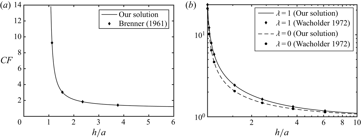
 $F'_D$ from (4.11) into (5.1). The comparative results have been depicted in figure 2(a,b); in figure 2(a), we have compared the
 $CF$ from our solutions with that reported by Brenner (Reference Brenner1961) for a solid particle; in figure 2(b), our results are compared with those of Wacholder & Weihs (Reference Wacholder and Weihs1972) for bubbles (
 $\lambda = 0$) and drops (
 $\lambda = 1$). Values of the other relevant parameters have been mentioned in the caption. In both the figures
 $CF$ has been plotted as a function of
 $h$, i.e. the distance of the drop from the wall. Notice that in figure 2(a), we have used a viscosity ratio of
 $\lambda = 10^6$ so that the drop effectively behaves as a solid particle.
(a) Comparison of the correction factor ( $CF$) to the hydrodynamic drag force on a solid sphere as obtained from our analysis to those reported by Brenner (Reference Brenner1961). We have plotted
 $CF$ as a function of
 $h$ and, because the particle is solid, we took
 $\beta = 0$; the other parameter is
 $\lambda = 10^6$. (b) Comparison of the same
 $CF$ with the ones reported by Wacholder & Weihs (Reference Wacholder and Weihs1972) in the absence of any surfactants (
 $\beta = 0$) at various distances (
 $h$) from the wall, for
 $\lambda = 0$ (bubble) and
 $\lambda = 1$ (liquid drop).

We observe a clear agreement between our results and those of Brenner in figure 2(a) and the ones from Wacholder & Weihs in figure 2(b), for the cases of bubble as well as the drop. There are some important points to note from these two figures. First, we observe that far away from the wall, i.e. when  $h\gg 1$,
 $CF\sim 1$, as expected. Second, the presence of the wall significantly enhances the hydrodynamic drag, as has been already established by previous studies (Brenner Reference Brenner1961; Wacholder & Weihs Reference Wacholder and Weihs1972). However, the drop starts experiencing this enhanced resistance only when it is really close to the wall, where
 $h \leq 2$. It may be further noted that increasing the viscosity ratio from
 $\lambda = 0$ to
 $\lambda \gg 1$ leads to increased drag and slower movement of the drop.
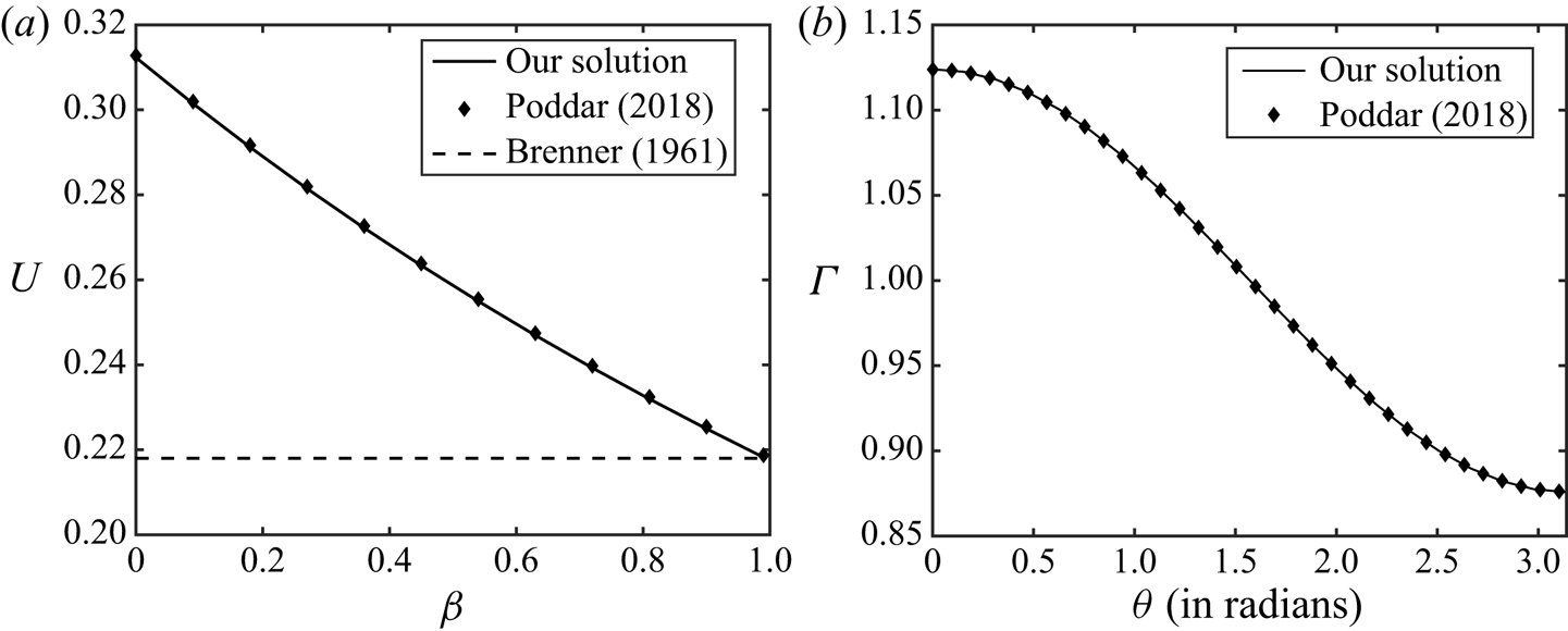
The comparison between our results and those reported in Poddar et al. (Reference Poddar, Mandal, Bandopadhyay and Chakraborty2018) for an unbounded surfactant-laden settling drop (the limit  $h\gg 1$) has been included in appendix B.
5.2. The flow field and the settling dynamics
We can get insight into the settling dynamics from either (4.12), which computes the settling velocity based on the instantaneous hydrodynamic drag, or by solving (4.13), which yields the position of the drop as a function of time, by carrying out an overall force balance on the same. We investigate the predictions of both of these equations here, while discussing the settling dynamics. Here, we would like to emphasize that the approach described in (4.13), coupled with the solutions using bispherical coordinates, has so far remained poorly addressed in the literature. First we shall probe into the effect of surfactants on the settling dynamics.
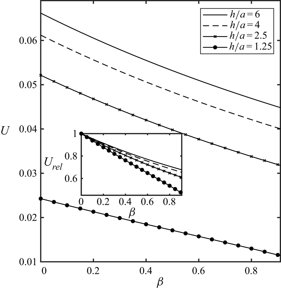
We begin with figure 3, where the settling velocity as computed from (4.12) as a function of  $\beta$ (coefficient of variation in the surface tension) has been depicted at four different positions of the droplet centre,
 $h = 6,4,2.5$ and
 $1.25$. In the inset we plot
 $U_{rel} = U/U_{\beta = 0}$ as a function of
 $\beta$ at those same positions. Noting that
 $U_{\beta = 0}$ denotes the velocity when the surface impurities have no effect on the droplet motion,
 $U_{rel}$ therefore documents the changes in the settling velocity, relative to the cases of pure drops. Values of all other relevant parameters have been mentioned in the caption.
Plot of droplet settling velocity ( $U$) as calculated from (4.12) as a function of
 $\beta$ for four different locations of the drop centre, given by
 $h = 6, 4, 2.5, 1.25$. In the inset
 $U_{rel}$, defined as
 $U_{rel} = U/U_{\beta =0}$, has been plotted as a function of
 $\beta$ at those same locations. Here
 $U_{rel}$ reflects how differently a surfactant laden drop behaves relative to one without any surface impurities. Other relevant parameters are given by
 $\lambda = 0.1$ and
 $k = 3$.

There are two very clear patterns that one can observe in figure 3. First, at all positions of the drop (i.e. for all values of  $h$), presence of surfactant slows down the settling velocity. Interestingly, the net amount by which the velocity changes (the
 $\Delta U$) roughly remains the same at all positions, as noted from the figure. The second point to observe is that closer the drop is to the wall, the smaller is its settling velocity, irrespective of the presence of surfactant. Both of these features are expected because the presence of surface impurities have been shown to slow down the motion of drops (Chen & Stebe Reference Chen and Stebe1996; Leal Reference Leal2007; Mandal et al. Reference Mandal, Ghosh and Chakraborty2016, Reference Mandal, Das and Chakraborty2017b; Poddar et al. Reference Poddar, Mandal, Bandopadhyay and Chakraborty2018) by resisting the fluid motion near the interface. This resistance arises because interfacial motion redistributes surfactants around the drop surface, as discussed later. For example, if the fluid velocity relative to the drop is towards the pole in the northern hemisphere (
 $\eta < {\rm \pi}/2$), it would lead to an accumulation of surfactants near the north pole (
 $\eta = 0$; also see figure 5c,d) and as a result, the surface tension there will be less as compared with that in the equatorial region. This would indicate that the surface tension gradient would effectively pull the fluid towards the equator by inducing Marangoni stress, leading to a resistance to the original background motion. A natural consequence of this is a slowing down of the fluid motion around the interface, which also leads to a smaller settling velocity of the drop itself. On the other hand, a smaller value of
 $h$ (i.e. when the drop is closer to the wall) results in a larger hydrodynamic drag on the drop, as already pointed out in figure 2 and, therefore, ultimately slows it down.
The inset of figure 3 (plot  $U_{rel}$ versus
 $\beta$) paints an interesting and explicit picture of how the presence of surfactant changes the settling velocity at different locations. Notice that the relative change compared with a pure drop (
 $\beta = 0$) is the largest when
 $h = 1.25$; in fact for
 $\beta = 0.9$ (surfactant strongly influences the surface tension), presence of surfactant changes the settling velocity by approximately 40 % relative to a drop with a pure interface. Notice, however, this relative change is much lower when the drop is located farther away from the wall. We therefore conclude that the influence of surfactant on the settling dynamics increases as the drop gets closer to the wall. In other words, the effect of surfactants on the settling velocity is the strongest very close to the bounding wall; the same is least influential when the drop is far away from the wall and the surrounding medium effectively behaves like an unbounded one.
A more complete description of the droplet settling dynamics is offered by (4.13), where we solve for  $h(t)$ and
 $\dot {h}(t)$ as functions of time, by also taking into account the acceleration of the droplet's centre of mass. More insight into the settling dynamics may then be obtained by investigating how the distance of the drop (
 $h(t)$) changes with time, as it is released from a certain height (denoted by
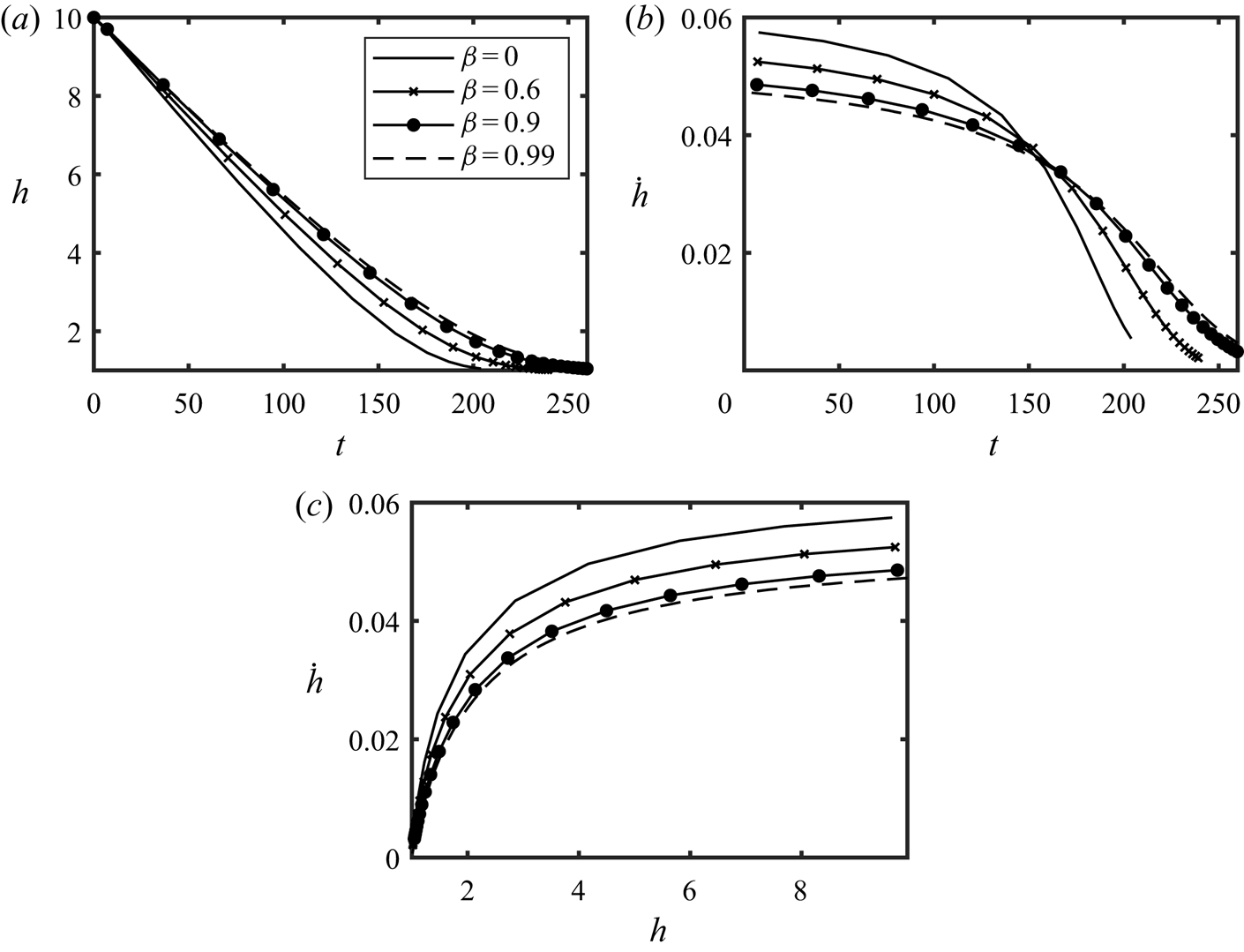
 $h_0$), in the presence of surfactants. The resulting variations are among the most important features emerging from the settling dynamics under consideration. Figure 4(a–c) demonstrate how the presence of surfactant changes the drop's position (
 $h(t)$) and its velocity (
 $|\dot {h}(t)|$) with time, when released from rest (
 $\dot {h}(t) = 0$) from an initial height
 $h_0 = 10$, for four different choices of
 $\beta = 0,0.6,0.9$ and
 $0.99$, wherein
 $\beta = 0.99$ represents the limiting case of a solid particle, without any internal motion (also see appendix B). Figure 4(a) shows how
 $h$ varies in time, figure 4(b) depicts the variations in the drop's velocity (
 $|\dot {h}(t)|$) with time and figure 4(c) plots
 $|\dot {h}(t)|$ versus
 $h(t)$, which is the phase plot of the settling dynamics.
The droplet settling dynamics as computed by solving (4.13), is depicted for four different choices of  $\beta = 0,0.6,0.9$ and
 $0.99$. Here
 $\beta = 0.99$ represents the limiting case of a solid particle. In panel (a)
 $h(t)$ versus
 $t$ has been plotted; in panel (b) the velocity of the drop,
 $|\dot {h}(t)|$ versus
 $t$ has been depicted, and in panel (c) the phase plot of
 $|\dot {h}(t)|$ versus
 $h(t)$ has been shown. For all values of
 $\beta$, the drop starts at
 $h_0 = 10$. Values of other relevant parameters are
 $\lambda = 1$,
 $k = 3$.

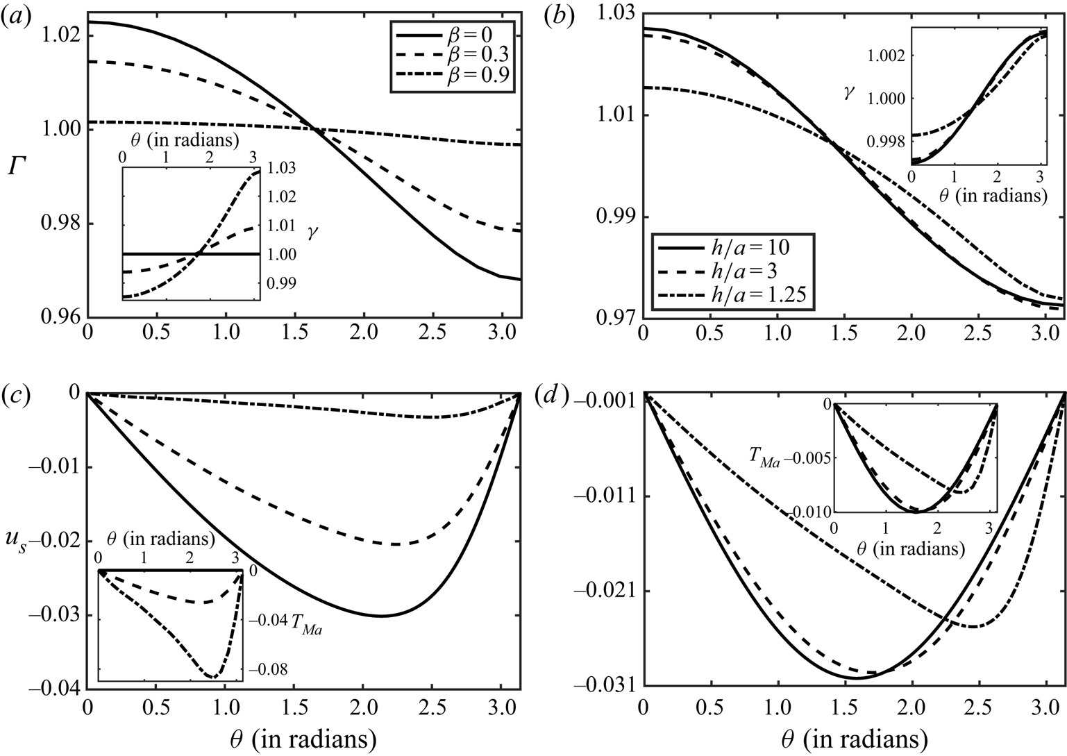
(a) Surfactant concentration ( $\varGamma$) as a function of
 $\theta$ for three values of
 $\beta = 0, 0.3, 0.9$ have been plotted, with
 $h = 1.5$. The inset figure plots the variation of surface tension (
 $\gamma$) versus
 $\theta$ for same parameters. The angle
 $\theta$ is the polar angle measured with respect to the centre of the drop. (b) Here
 $\varGamma$ versus
 $\theta$ is plotted at three different locations of the drop,
 $h = 1.25,3,10$, for
 $\beta = 0.1$. The inset shows the variation in
 $\gamma$ versus
 $\theta$ at same locations. (c) Interface velocity (
 $u_s = u^{(2)}_{\eta }$) as a function of
 $\theta$ for three values of
 $\beta = 0, 0.3, 0.9$ have been plotted, with
 $h = 1.5$. The inset figure plots the variation of Marangoni stress (
 $T_{Ma} = \omega h_1({\partial \varGamma ^{(1)}_1}/{\partial \eta })$) versus
 $\theta$ for same parameters. (d) Here
 $u_s$ versus
 $\theta$ is plotted at three different locations of the drop,
 $h = 1.25,3,10$, for
 $\beta = 0.1$. The inset shows the variation in
 $T_{Ma}$ versus
 $\theta$ at same locations. Other relevant parameters are
 $\lambda = 0.1$,
 $k = 3$,
 $Ca_s = 0.3$ for all the plots.

Figure 4(a–c) overall agree exactly with what is observed in figure 3. We note from figure 4(a) that  $h$ decreases the fastest when
 $\beta = 0$, i.e. when the surfactant does not influence fluid motion, while the slowest settling occurs for
 $\beta = 0.99$, i.e. when the internal fluid motion is arrested and the droplet behaves like a solid particle. Generally, we notice that increasing
 $\beta$ slows down the settling velocity; this influence of the surfactant is maximized when
 $\beta =0.99$, i.e. when variations in surface tension across the interface are large. We therefore conclude that presence of stronger internal fluid motion results in lower hydrodynamic drag on the drop (Wacholder & Weihs Reference Wacholder and Weihs1972). Figure 4(b), on the other hand, indicates that the drop continually decelerates while settling, as attributable to an ever increasing hydrodynamic drag force. At the same time, we also note that presence of surfactants actually suppresses the rate at which the drop decelerates, as it moves downwards. As a result, although a drop without surfactants (
 $\beta = 0$ curve) moves much faster initially, after a certain amount of time, it would move slower than a surfactant-laden drop because of the rapid deceleration it experiences combined with the fact that at that given instant it would be closer to the wall as compared with a drop with surface impurities, thus also experiencing larger hydrodynamic drag. Finally, figure 4(c) outlines how the drop's settling velocity changes as a function of its distance from the wall. This figure reveals that, although the drop continuously slows down while settling, when it is relatively farther away from the wall (
 $h\geq 4$), its velocity shows little change. Most of the deceleration occurs only very close to wall, for
 $h\leq 3$ and in this region the drop decelerates very rapidly, as is evident from the figure. Notice that the general features of the drop's motion persist irrespective of whether surface impurities are present. Hence, we conclude that the presence of surfactant does not fundamentally alter the settling dynamics of the drop. Although its effect is the most prominent close to the wall, the primary influence of surfactants is to slow down the drop.
We end this subsection by exploring how the surfactant concentration and the interfacial velocity vary, as the drop settles towards the wall. Recall that the surfactant concentration can be computed from (4.9), by numerically integrating it as discussed in § 4.1. The surface tension  $\gamma$ is defined as (see § 3)
 $\gamma = 1-\beta (1-\beta )^{-1}\varGamma _1$. On the other hand, the interfacial velocity is defined as
 $u_s = u^{(2)}_{\eta }$, see (3.7). The Marangoni stress on the drop surface may be defined as
 $T_{Ma} = \omega h_1({\partial \varGamma ^{(1)}_1}/{\partial \eta })$, refer to (4.5c).
In figure 5(a,b), we plot the surfactant concentration ( $\varGamma$) as a function of
 $\theta$ on the drop interface for two different scenarios. In figure 5(a), we show the effect of
 $\beta$ on the variations in
 $\varGamma$ at a fixed position of the drop (
 $h = 1.5$); in figure 5(b), we demonstrate how the surfactant redistributes itself as the drop moves downwards by plotting
 $\varGamma$ versus
 $\theta$ at three different locations of the drop, given by
 $h = 10,3$ and
 $1.25$. In the inset, we show how the surface tension varies across the interface, for the situations described in the main figures. In figure 5(c,d), variations in the interfacial velocity with
 $\theta$ have been depicted under the same conditions as those in figures 5(a) and 5(b), respectively. In the insets, variations in the Marangoni stresses (
 $T_{Ma}$) as a function of
 $\theta$ have been shown under those same conditions. In all the panels,
 $\theta$ is the polar angle defined in a spherical coordinate system with its origin fixed at the drop centre. Values of other relevant parameters have been mentioned in the caption.
Figure 5(a) demonstrates how the surfactant is redistributed relative to the drop, as governed by the interfacial velocity,  $u_{\eta }^{(2)}$. From figure 5(c) we note that the relative velocity at the drop interface is directed towards the north pole from the south pole through the equator (
 $\eta \approx {\rm \pi}/2$), which explains why surfactants tend to get accumulated near the north pole, as shown in figure 5(a). As a consequence the factor
 ${\partial \varGamma ^{(1)}}/{\partial \eta } < 0$ which results in
 $T_{Ma}<0$, as shown in the inset of figure 5(c). This leads to an ever-decreasing surface tension as one moves from the south pole towards the north, as shown in the inset of figure 5(a), which opposes the interfacial motion of the fluids between the poles. The above argument explains why increasing
 $\beta$ makes the surfactant concentration more uniform across the interface, as observed in figure 5(a). Larger
 $\beta$ would result in larger variations in surface tension across the interface; recall that this non-uniformity in the surface tension opposes fluid motion along the interface and thus increasing
 $\beta$ results in a reduction in the interfacial velocity,
 $u_s$. Since
 $u_s$ is mainly responsible for redistributing the surfactants between the poles, a reduction in its value would naturally indicate weaker surfactant advection, hence leading to more uniform concentrations across the interface. It is also interesting to note from figure 5(a) that
 $\varGamma$ is slightly asymmetric with respect to the equator (
 $\theta = {\rm \pi}/2$); observe that near the south pole of the drop,
 $|\varGamma _1|$ (recall that
 $\varGamma _1 = \varGamma -1$, see § 3) is slightly higher than the north pole. This slight asymmetry comes about because the presence of the wall and the surfactant together breaks the fore-and-aft symmetry that prevails in an unbounded suspending medium.
Figure 5(b), on the other hand, demonstrates how the surfactant gets redistributed while the drop settles towards the wall, for a fixed value of  $\beta = 0.1$. One of the major takeaways from this figure is that
 $\varGamma _1(\theta )$ becomes more asymmetric around the equator as the droplet nears the wall. Notice that when
 $h = 10$,
 $|\varGamma _1|$ is essentially symmetric around
 $\theta = {\rm \pi}/2$, akin to a drop in an unbounded suspending medium and
 $\varGamma = 1$ almost exactly at the equator. However, as
 $h$ decreases,
 $\varGamma (\theta )$ becomes increasingly asymmetric and the location of
 $\varGamma = 1$ gradually shifts towards the southern hemisphere. The asymmetry in
 $|\varGamma _1(\theta )|$ is most prominent at
 $h = 1.25$, where the larger extent of concentration depletion near the south pole is clearly visible. The reason for this becomes clear from figure 5(d), where it is observed that the interfacial velocity distribution becomes asymmetric and the location of the maxima in
 $u_s$ shifts towards the south pole, as the drop approaches the wall. This naturally results in stronger advection currents of surfactant in the southern hemisphere, which ultimately leads to larger surfactant depletion in that region, as noted from figure 5(b). However, the overall deviation in the surfactant concentration from equilibrium (i.e.
 $\varGamma _1$) still gets smaller as the drop gets closer to the wall. The reason for this may be attributed to an overall reduction in the fluid motion, the main driving force behind the non-uniformity in
 $\varGamma$, because of an ever-decreasing settling velocity of the drop as it nears the wall. This trend continues in the final stages of settling as well, wherein the surfactant concentration becomes almost uniform across the interface – see § S4 in the supplementary material for quantitative details. At the same time, strong correlation between
 $u_s$ and
 $T_{Ma}$ in the inset of figure 5(d) is to be noticed, which stems from the redistribution of surfactants caused by the interfacial velocity.
5.3. Droplet deformation and film drainage
The deformed shape of the drop may be computed from the analysis mentioned in § 4.3. For representing the results, we quantify the deformation by defining a modified aspect ratio ( $\mathcal {AR}$) as follows:
 \begin{equation} \mathcal{AR} = \frac{2\rho_{{max}}}{H_{{v}}}, \end{equation}
where,  $\rho _{{max}}$ is the maximum width of the drop measured from the centre and
 $H_{{v}}$ is the height of the drop along its centreline,
 $\rho = 0$. Another quantity of interest that profoundly influences the deformation is the total normal stress difference across the drop interface and is defined as
 \begin{equation} \Delta T_{\xi\xi} = \lambda p_2-p_1 + \tau^{(1)}_{\xi\xi}-\lambda\tau^{(2)}_{\xi\xi}. \end{equation}
It is important to note that variations in  $\Delta T_{\xi \xi }$ dictate how the drop interface (or, any interface, for that matter) would deform.
We begin with figure 6(a–d), where the effect of surfactant on  $\mathcal {AR}$ and
 $\Delta T_{\xi \xi }$ have been showcased. In figure 6(a),
 $\mathcal {AR}$ is plotted at varying distances from the wall, for three different values of
 $\beta = 0,0.6$ and
 $0.9$. The inset magnifies the region of the graph where crossovers occur between the
 $\mathcal {AR}$s corresponding to the different values of
 $\beta$. In figure 6(b),
 $\Delta T_{\xi \xi }$ versus
 $\theta$ is plotted for a pure interface (represented by
 $\beta = 0$) at three different locations,
 $h = 50,3$ and
 $1.5$. Figure 6(c,d) demonstrate variations in
 $\Delta T_{\xi \xi }$ versus
 $\theta$ for a surfactant-laden drop at two fixed locations,
 $h = 1.5$ and
 $h = 1.05$, respectively, for three choices of
 $\beta = 0,0.6$ and
 $0.9$. The definition of
 $\theta$ here remains the same as that in figure 5. It is well documented (Leal Reference Leal2007; Poddar et al. Reference Poddar, Mandal, Bandopadhyay and Chakraborty2018) that a freely settling drop in an unbounded surrounding medium does not deform, even in the presence of surface impurities. However, deformations do occur when a bounding wall is present, especially when the drop is close to the wall (Wacholder & Weihs Reference Wacholder and Weihs1972). The reason is that the presence of a wall leads to excess stresses below the drop, which tend to squash the drop from the bottom (Wacholder & Weihs Reference Wacholder and Weihs1972; Pozrikidis Reference Pozrikidis2001) and also from the top, but to a lesser extent. As a result, the drop would tend to get elongated horizontally and hence we should have
 $\mathcal {AR} \geq 1$. This is exactly what we observe from figure 6(a), wherein it may be noted that
 $\mathcal {AR}$ monotonically increases as
 $h$ decreases. Recall that
 $\lim _{h\rightarrow \infty }\mathcal {AR} = 1$, as discussed earlier. Further observe that, the presence of surfactant slightly augments the deformation as long as the drop is beyond a certain distance from the wall (for example, when
 $h\geq 1.4$ for
 $\beta = 0.6$); similar conclusions have also been reached in previous studies (Mandal et al. Reference Mandal, Ghosh and Chakraborty2016). The reason may be attributed to a reduction in surface tension as well as its non-uniformity, caused by the surface impurities; recall that the surface tension usually helps the fluid counteract the stress difference across the interface. However, sufficiently close to the wall (the exact values of
 $h$ depends on
 $\beta$), we note that the surface impurities actually suppress the deformation, albeit by a small amount, as evident from the inset of figure 6(a). For instance, observe from the inset that for
 $h<1.1$,
 $\{\mathcal {AR}_{\beta = 0.9},\mathcal {AR}_{\beta = 0.6}\} < \mathcal {AR}_{\beta = 0}$. The reason for such reductions in
 $\mathcal {AR}$ may be attributed to an accompanying reduction in the drop's velocity, which results in a decrease in the overall viscous stresses on the interface, leading to smaller deformations and hence smaller
 $\mathcal {AR}$.
(a) Plot of  $\mathcal {AR}$ versus
 $h$ for three different
 $\beta$ values (
 $\beta = 0,0.6$ and
 $0.9$). In the inset, crossover between the
 $\mathcal {AR}$ for different
 $\beta$-values have been shown. (b) Variation in the total normal stress difference (
 $\Delta T_{\xi \xi } = \lambda p_2-p_1 + \tau ^{(1)}_{\xi \xi }-\lambda \tau ^{(2)}_{\xi \xi }$) for a pure drop (no surfactant,
 $\beta = 0$) versus
 $\theta$ at three different positions,
 $h = 50,3$ and
 $1.5$ (c) Total normal stress difference (
 $\Delta T_{\xi \xi }$) versus
 $\theta$ at
 $h = 1.5$ for three different values of
 $\beta$ (
 $\beta = 0,0.6$ and
 $0.9$). (d) Total normal stress difference (
 $\Delta T_{\xi \xi }$) versus
 $\theta$ at
 $h = 1.05$, with other parameters remaining same as those in panel (c). Values of other relevant parameters are
 $Ca_s = 0.4$,
 $\lambda = 0.1$,
 $k = 3$. Note that
 $\theta$ here has the same definition as mentioned in figure 5.

Figure 6(b–d) helps us gain more insight into the interfacial deformation by depicting the variations in the normal stress difference across the interface. In figure 6(b), where a surfactant-free drop is analysed, we note how the stress difference changes as the drop settles downwards. At  $h = 50$, where the effect of the wall is essentially absent, normal stress difference remains constant along the interface, which indicates that the interface remains spherical (constant curvature) and the drop does not deform. Closer to the wall, however,
 $\Delta T_{\xi \xi }$ is non-uniform and hence would cause deformation. Notice from figure 6(b) that
 $\Delta T_{\xi \xi }$ is slightly lower towards the poles (
 $\theta = 0$ and
 ${\rm \pi}$) as compared with the equator and is the lowest near the south pole. As a result, the curvature near the poles is expected to be smaller, thus indicating that the drop would tend to become flatter in the polar regions. For this same reason and to conserve the total volume, the drop would bulge out near the equator and hence would result in
 $\mathcal {AR}>1$ – see figure 7 for a visual representation. It is clear that the normal stress difference becomes more non-uniform closer to the wall, which results in increasingly larger deformation, as shown in figure 6(a). Figure 6(c) reveals how the presence of surfactant changes the normal stress difference across the interface. Notice that overall distribution of
 $\Delta T_{\xi \xi }$ is similar to a pure interface; it is the largest near the equator and gradually drops towards the poles. However, there are three major differences between the
 $\Delta T_{\xi \xi }$ shown in figure 6(b,c): (i) in the presence of surfactants, the stress difference is the lowest at the north pole; (ii) the maximum
 $\Delta T_{\xi \xi }$ does not occur at the equator, but rather in the southern hemisphere (
 $\theta > {\rm \pi}/2$); and (iii) in presence of surfactants
 $\Delta T_{\xi \xi }$ gets augmented. Since the surface tension is the largest near the south pole (see figure 5b) this would make the drop flatter near that region. At the same time, the bulge near the equator would increase because of the larger stress difference. A combined influence of these changes results in a larger
 $\mathcal {AR}$ in the presence of surfactants. In figure 6(d), however, we notice that very close to the wall (here,
 $h = 1.05$), the surfactants cause almost no changes in
 $\Delta T_{\xi \xi }$, except near the south pole (
 $\theta = {\rm \pi}$), where
 $\Delta T_{\xi \xi }$ is slightly higher than that of a pure interface. At the same time, the surface tension there is also larger because of surfactant depletion, as shown in figure 5(b), while on the rest of the interface,
 $\Delta T_{\xi \xi }$ stays nearly constant. A combination of these two factors mentioned above ultimately leads to smaller deformation, thus resulting in smaller
 $\mathcal {AR}$ values as compared with a surfactant-free drop.
Deformed shape of the drop from the leading-order theory at four different locations  $h = 2,1.5,1.1$ and
 $1.005$. The presence of surfactant has been taken into account here with
 $\beta = 0.9$. Other relevant parameters are
 $Ca_s = 0.5$,
 $\lambda = 0.1$,
 $k = 3$. The original spherical shape is denoted by the red dashed line.

On a more general note, we observe from figure 6 that the deformation is actually quite small, since  $\mathcal {AR}$ changes by only approximately 6 %, even when
 $Ca_s = 0.4$. As a result, the leading-order theory, which assumes the drop remains spherical for capturing the flow dynamics, is expected to be reasonably accurate, precisely because the drop shape actually does not deviate significantly from a sphere, at least when
 $Pe\sim O(Ca_s)$ and
 $Ca_s< O(1)$. Existing literature (Steinhaus et al. Reference Steinhaus, Spicer and Shen2006; Hendrix et al. Reference Hendrix, Manica, Klaseboer, Chan and Ohl2012) also shows that small drops do remain more or less spherical, even when they are approaching a bounding wall.
In figure 7(a–d), the deformed shape of a surfactant-laden settling drop has been shown at various distances from the wall, while values of all relevant parameters have been mentioned in the caption. The red dashed line denotes the undeformed spherical drop. We observe that the drop shapes in the present figure exactly agree with what was discussed in relation to figure 6. Far away from the wall, the drop remains perfectly spherical, as expected of a freely settling drop in an otherwise unbounded medium. As the drop inches closer to the wall (at  $h = 1.1$ in figure 7c), the deformation becomes visible, wherein the drop flattens from the top and the bottom, while a small bulge is observed near the equator. The flattening is more prominent at the bottom of the drop, which is closer to the wall. At a distance very close to the wall (
 $h = 1.005$, see figure 7d), an axisymmetric dimple forms at the bottom of the drop; this feature has also been reported in the past experimental studies (Joye et al. Reference Joye, Hirasaki and Miller1992; Clasohm et al. Reference Clasohm, Connor, Vinogradova and Horn2005; Horn, Asadullah & Connor Reference Horn, Asadullah and Connor2006). The large interfacial deformations (including dimple formation) in the final stages of the settling as shown in figure 7, profoundly alter the drainage rate of the liquid film residing between the drop and the solid wall, as we discuss shortly. The genesis of the deformation observed has already been discussed in detail in § 4.3 and in relation to figure 6.
We end our discussions by looking into how the film thickness between the drop and solid surface varies with time in the presence of surface impurities, and in the process compare our predictions with the existing literature. We define the film thickness as
 \begin{equation} \Delta h(\rho,t)= h(t)-\mathcal{L}(\eta,t)\left\{1-Ca_s f(\eta,t)\left(\frac{\sinh\alpha(t)}{\cosh\alpha(t)-\cos\eta}\right)\right\},\quad \forall\ \eta>{\rm \pi}/2, \end{equation}
where  $\mathcal {L}(\eta ,t) = ({1-\cosh \alpha (t)\cos \eta })/({\cosh \alpha (t)-\cos \eta })$,
 $\alpha (t) = \cosh ^{-1}(h(t))$ (see § 4) and
 $\Delta h_{min}(t) = \min \{\Delta h(\rho ,t)\}$ is the minimum thickness of the film (see figure 8). Notice that the
 $O(Ca_s)$ deformation has been accounted for in estimating the film thickness, as described above. Film drainage, which investigates how
 $\Delta h$ varies with time in the final stages of settling, has been extensively studied, both theoretically (Jones & Wilson Reference Jones and Wilson1978; Lin & Slattery Reference Lin and Slattery1982; Hartland et al. Reference Hartland, Yang and Jeelani1994) and experimentally (Joye et al. Reference Joye, Hirasaki and Miller1992; Steinhaus et al. Reference Steinhaus, Spicer and Shen2006; Aarts & Lekkerkerker Reference Aarts and Lekkerkerker2008) over the years. Cox & Brenner (Reference Cox and Brenner1967), using Lubrication theory, have previously shown that the minimum film thickness (
 $\Delta h_{min}$) between a flat wall and an approaching solid spherical particle (radius
 $a$) varies as
 $\Delta h'_{min} = \Delta h'_0 \exp \left ({-F'(t'-t'_0)/6{\rm \pi} \mu _1 a^2}\right )$, when the particle is acted upon by a constant force
 $F'$ and
 $\Delta h' \ll a$, while
 $\Delta h'_0$ is the minimum film thickness at time
 $t' = t'_0$. This can be compared with our solutions by enforcing
 $F'= ({4}/{3}){\rm \pi} a^3 (\rho _2 - \rho _1)g$ and taking the limit
 $\beta \rightarrow 1$ (solid particle limit), while ignoring deformation (
 $f(\eta ,t)\rightarrow 0$). The minimum film thickness
 $\Delta h_{min}$ can be expressed in dimensionless form by using the characteristic scales mentioned in § 3 and takes the following form:
 \begin{equation} \Delta h_{min}(t) = \Delta h_0 \exp\left({-(t - t_0)/6{\rm \pi}}\right). \end{equation}
(a) Plot of minimum film thickness ( $\Delta h_{min}$) versus
 $t$ for
 $\beta = 0,0.3,0.6$ and
 $0.99$ (solid particle limit,
 $f(\eta ) = 0$). Other relevant parameters are
 $\lambda =0.1$,
 $Ca_s = 0.1$,
 $k=3$. The red dashed line represents solution by Cox & Brenner (Reference Cox and Brenner1967) for solid particles. In the inset, final stages of film drainage for the case of drops have been shown. (b) Plot of the film thickness
 $\Delta h$ versus
 $\rho$ in the final stages of settling, for three different locations of the drop centre,
 $h = 1.1,1.01,1.001$ and
 $\beta = 0.1$; other parameters are same as those in panel (a). Only part of the bottom surface of the drop has been shown here (
 $\eta >{\rm \pi} /2$). (c) Same as panel (b), with
 $Ca_s = 0.4$ instead of
 $0.1$, for further clarification.

Figure 8(a) demonstrates the variations in the minimum film thickness ( $\Delta h_{min}$) with time, for four different choices of
 $\beta = 0, 0.3, 0.6$ and
 $0.99$. The graph of
 $\beta = 0.99$ represents the film drainage for a solid particle and thus we have enforced
 $f(\eta ,t) = 0$ for this case (no deformation). In figure 8(b),
 $\Delta h$ as a function of radial distance
 $\rho$ has been plotted in the final stages of approach for
 $Ca_s = 0.1$, wherein the bottom part of the drop has been depicted for three different
 $h = 1.1,1.01$ and
 $1.001$ and
 $\beta = 0.1$. Figure 8(c) also shows the same quantity, albeit for a larger capillary number,
 $Ca_s = 0.4$, resulting in larger deformation. In the inset of figure 8(a), behaviour of
 $\Delta h_{min}$ at large times have been highlighted, for various values of
 $\beta$ (see the legend). We have computed
 $\Delta h$ by solving
 $\textrm {d}h/\textrm {d}t = -U$, where
 $U$ is evaluated from (4.12) and
 $\Delta h$ is then estimated from (5.4). Values of all other relevant parameters have been mentioned in the caption.
We first notice that for  $\beta = 0.99$, i.e. in the limit of solid particle, clear agreement can be observed between our results and those of Cox & Brenner (red dashed line), after the film thickness
 $\Delta h_{min}$ drops below
 $0.1$. Therefore, in the limiting case of a solid particle,
 $\Delta h$ decays exponentially with time. Shifting our attention to droplets (lower values of
 $\beta$), we note that the decay in
 $\Delta h$ can be divided into two distinct regimes. First, in the ‘buoyancy dominated regime’, exponential decay in
 $\Delta h_{min}$, similar to a solid particle is observed, albeit only up to a certain
 $\Delta h_{min}\sim O(10^{-1})$. The second regime, below
 $\Delta h \sim O(10^{-1})$, may be classified as ‘deformation dominated regime’, where the drainage rate slows down drastically, because of deformation of the bottom surface of the drop. This phenomenon can be observed from figure 8(b), where the bottom surface of the drop at various locations of the drop centre has been shown. It is clear that the drop first flattens from the bottom (see figure 7), following which a ‘dimple’ forms at the centre of the bottom surface, as it moves closer to the wall. As a result, the radial position of
 $\Delta h_{min}$ shifts towards the outer edges of the drop, leading to a so-called ‘ring formation’. We would like to point out that both ‘dimple’ formation as well as the outward shift in the radial position of
 $\Delta h_{min}$ have been observed experimentally (Connor & Horn Reference Connor and Horn2003; Hendrix et al. Reference Hendrix, Manica, Klaseboer, Chan and Ohl2012; Zhang et al. Reference Zhang, Manica, Tchoukov, Liu and Xu2017).
From the inset of figure 8(a) it becomes evident that in the deformation dominated regime, the decay in  $\Delta h_{min}$ becomes algebraic from exponential. In fact for a pure drop with
 $\lambda \ll 1$ and
 $\beta = 0$, we observe
 $\Delta h_{min} \sim t^{-s}$, where
 $s = 1/2$, represented by the dashed blue line in the inset. Similar scaling has been previously suggested (see for instance the work of Hewitt et al. (Reference Hewitt, Fornasiero, Ralston and Fisher1993) and the citations therein) in relation to film drainage between air bubbles and solid surfaces. However, the viscosity of the drop as well as the presence of solutes in the bulk fluid may significantly alter this scaling. Similarly, we observe from figure 8(a) that this scaling also changes when surface impurities are present, implying
 $\beta >0$. In particular, for higher values of
 $\beta$ such as
 $0.6$, we can even observe non-monotonic decay in
 $\Delta h_{min}$. At the same time, no universal scaling (e.g. a
 $t^{-1/2}$ decay) is observed for
 $\Delta h_{min}$ in the presence of surfactants. Moreover, the inset clearly demonstrates that the initiation of the deformation dominated regime gets delayed when
 $\beta >0$. This is accompanied by a slow transition of the film drainage rate from algebraic decay for drops (
 $t^{-1/2}$ for bubbles with pure interface) to exponential decay for solid particles. The time span of the second regime shown in the figure is relatively small, precisely because of extremely slow drainage rate, which slows down the droplet motion considerably. Snapshots of flow patterns at different stages of settling, including the squeezing out of the film between the drop and the wall during the final moments have been discussed in § S4 of the supplementary material. When the film thickness becomes extremely small (
 $\Delta h_{min}\sim O(10\ \text {nm})$), non-hydrodynamic effects such as disjoining pressure (Hu & Sun Reference Hu and Sun2013) start playing important roles. Since ours is a pure hydrodynamics based analysis, these final stages of film drainage cannot be captured using the formulation outlined herein.
6. Conclusion
The settling dynamics of a surfactant-laden drop towards a solid wall is analysed here. To this end, we consider the ‘insoluble surfactant’ limit, wherein the interfacial transport of the surfactants dominate over the slow adsorption–desorption from the bulk. We have further assumed, with a posteriori validation, that the drop deformation is small on account of low capillary number ( $Ca_s$), which allowed us to carry out asymptotic analysis for evaluating the resulting velocity field and the settling dynamics. We consider weak interfacial advection of the surfactants (quantified by
 $Pe$), so that
 $Pe \sim O(Ca_s)$. It was assumed that the surfactant's primary influence on the flow comes from altering the surface tension. We employed a bipolar coordinate system and subsequently derived semianalytical solutions for the stream function and the surfactant concentration, both of which are represented as infinite series. The solutions for the velocity field were subsequently used to compute the hydrodynamic drag on the drop, which may be utilized to investigate the drop's settling velocity and its overall settling dynamics. The velocity fields were also used to compute the leading-order deformation to the original spherical shape of the drop, which was subsequently used to probe into film drainage in the final stages of settling. We have extensively validated our analysis by comparing the special cases of our results to a number of previously reported studies in the literature.
A number of important conclusions may be drawn from our analysis. First we showed that the presence of surface impurities slows down the drop at all distances from the wall. That being said, the effect of the surfactants on the drop's velocity is most prominent when it approaches the wall. As a result, when left freely from a given height, a surfactant-laden drop would settle much slower as compared with a pure drop. It is observed that the drop quickly decelerates once it comes within a certain distance from the wall, because of rapidly increasing hydrodynamic drag. We establish that the effect of surfactants essentially depends on the parameter  $\beta$, which controls its influence on the surface tension between the two fluids. Our study also revealed a number of interesting facets of the surfactant concentration distribution; we showed that near the wall, the surfactant distribution around the interface becomes considerably asymmetric, with comparably larger depletion near the south pole and more modest increases in concentration elsewhere.
We established that, away from the wall, the presence of surface impurities results in a larger stress difference across the interface, thus enhancing the deformation, although the fundamental nature of the deformation does not change. However, sufficiently close to the wall, the presence of surfactants causes a slight reduction in the deformation. The drop essentially remains undeformed far away from the wall. As it inches closer to the wall, it gets flattened from both top and bottom (more so from the bottom) and bulges out slightly in the middle. In the final stages of settling, an axisymmetric dimple forms at the bottom, a phenomenon that has also been observed experimentally. Our analysis can also successfully capture a significant portion of the film drainage in the final stages of settling, where deformation becomes a dominant factor as it significantly slows down the drainage rate. Presence of surfactant, however, delays the initiation of this deformation dominated stage in film drainage. We show that the absolute deformation remains small, even for relatively modest  $Ca_s$ values, and the overall effect of surfactants on the deformation is very limited.
Supplementary material
Supplementary material is available at https://doi.org/10.1017/jfm.2020.1101.
Funding
S.N.J. and U.G. are grateful to the Department of Science and Technology (DST), Govt. of India, for providing financial support for this work, through the Core Research Grant no. CRG/2019/000241.
Declaration of interests
The authors report no conflict of interest.
Appendix A. Analysis of the boundary conditions: the flow field and normal stress balance
A.1. Derivation of the linear system of algebraic equations
In this section we analyse the boundary conditions (4.5), subject to the solutions specified in (4.3), (4.4) and (4.9). To this end, we note the following:
 \begin{gather} \mathcal{S}_i = \psi_i(\cosh\xi-\cos\eta)^{{3}/{2}}=\sum_{n=0}^{\infty} W^{(i)}_n(\xi)C^{-{1}/{2}}_{n+1}(\cos\eta);\quad i = 1, 2, \end{gather}
 \begin{gather}\boldsymbol{U} = -U\hat{\boldsymbol{i}}_z;\quad \hat{\boldsymbol{i}}_z\boldsymbol{\cdot}\hat{\boldsymbol{i}}_{\xi} = -h_2\frac{\partial \rho}{\partial \eta}; \quad \hat{\boldsymbol{i}}_z\boldsymbol{\cdot}\hat{\boldsymbol{i}}_{\eta} = h_1\frac{\partial \rho}{\partial \xi}. \end{gather}
Using (A1a) in combination with (4.2a,b), the boundary conditions (4.5) and the surfactant transport equation (3.15) may be simplified as (at  $\xi = \alpha$)
 \begin{gather} \mathcal{S}_1 = \tfrac{1}{2}Uc^2\sin^2\eta (\cosh\xi - \cos\eta)^{-{1}/{2}};\quad \mathcal{S}_2 = 0, \end{gather}
 \begin{gather}\frac{\partial \mathcal{S}_1}{\partial \xi}- \frac{\partial \mathcal{S}_2}{\partial \xi} = \frac{\partial}{\partial \xi}\left\{\frac{1}{2}Uc^2\sin^2\eta(\cosh\xi - \cos\eta)^{-{1}/{2}}\right\},\\ \frac{\partial^2 \mathcal{S}_1}{\partial \xi^2} - \lambda\frac{\partial^2 \mathcal{S}_2}{\partial \xi^2} + \frac{\omega}{(\cosh\xi - \cos\eta)} \sum_{n=0}^{\infty} Z^{*}_nC^{-{1}/{2}}_{n+1}(\cos\eta)\nonumber\\ = \frac{\partial^2}{\partial \xi^2}\left\{\frac{1}{2}Uc^2\sin^2\eta(\cosh\xi - \cos\eta)^{-{1}/{2}}\right\},\end{gather}
 \begin{gather}\frac{\partial \mathcal{S}_1}{\partial \xi} - \frac{1}{c}\sum_{n=0}^{\infty} Z^{*}_nC^{-{1}/{2}}_{n+1}(\cos\eta) = \frac{\partial}{\partial \xi}\left\{-\frac{3}{2}Uc^2\sin^2\eta(\cosh\xi - \cos\eta)^{-{1}/{2}}\right\}. \end{gather}
The boundary condition at the wall ( $\xi = 0$), as well as the far-field condition, simplifies to
 \begin{equation} \mathcal{S}_1 = 0; \quad \frac{\partial \mathcal{S}_1}{\partial \xi} = 0. \end{equation}
Equations (A2) and (A3) may be converted to a set of algebraic equations for computing the unknown constants  $A^{*}_n$ to
 $Z^{*}_n$,
 $\forall n$, using the orthogonality properties of the Gegenbauer polynomials. This orthogonality condition is given by Leal (Reference Leal2007)
 \begin{equation} \int_{-1}^{1}\frac{C^{-{1}/{2}}_{n+1}(x)C^{-{1}/{2}}_{k+1}(x)}{1-x^2} \,{\textrm{d}x} = \frac{2\delta_{nk}}{n(n+1)(2n+1)}. \end{equation}
In addition, the following identity would also be useful (Brenner Reference Brenner1961):
 \begin{gather} \frac{\sin^2\eta}{(\cosh\xi - \cos\eta)^{{1}/{2}}} = \sum_{n=0}^{\infty}\frac{n(n+1)}{\sqrt{2}}\left[ \frac{\exp\left({-\left(n-\frac{1}{2}\right)\xi}\right)}{n-\frac{1}{2}}\right.\nonumber\\ \left. - \frac{\exp\left({-\left(n+\frac{3}{2}\right)\xi}\right)}{n+\frac{3}{2}} \right]C^{-{1}/{2}}_{n+1}(\cos\eta). \end{gather}
Since for every  $n$, there are seven constants, (A2) and (A3) finally yield a set of
 $7N$ linear algebraic set of equations, as follows (for
 $0\leq n \leq N$):
 \begin{gather} A_n + C_n = 0, \end{gather}
 \begin{gather}B_n(2n-1) + D_n(2n+3) = 0, \end{gather}
 \begin{gather}E_n \mathcal{L}_n + F_n \hat{\mathcal{L}}_n = 0, \end{gather}
 \begin{gather}A_n\mathcal{N}_n + B_n\hat{\mathcal{N}}_n + C_n\mathcal{P}_n + D_n\hat{\mathcal{P}}_n = \mathcal{M}_n\left[\frac{\mathcal{L}_n}{(2n-1)} - \frac{\hat{\mathcal{L}}_n}{(2n+3)}\right],\end{gather}
 \begin{gather}(2n-1)\left\{A_n\hat{\mathcal{N}}_n + B_n\mathcal{N}_n + E_n\mathcal{L}_n\right\} + (2n+3)\left\{C_n\hat{\mathcal{P}}_n + D_n\mathcal{P}_n + F_n\hat{\mathcal{L}}_n\right\}\nonumber\\ = \mathcal{M}_n[-\mathcal{L}_n+\hat{\mathcal{L}}_n], \end{gather}
 \begin{gather}(2n-1)\left\{A_n\hat{\mathcal{N}}_n + B_n\mathcal{N}_n\right\} + (2n+3) \left\{C_n\hat{\mathcal{P}}_n + D_n\mathcal{P}_n\right\} -\frac{2Z_n}{c} = 3\mathcal{M}_n[\mathcal{L}_n-\hat{\mathcal{L}}_n],\end{gather}
 \begin{gather}(2n-1)^2\left\{A_n\mathcal{N}_n + B_n\hat{\mathcal{N}}_n - \lambda E_n \mathcal{L}_n\right\} + (2n+3)^2\left[C_n\mathcal{P}_n + D_n\hat{\mathcal{P}}_n - \lambda F_n\hat{\mathcal{L}}_n\right]\nonumber\\ + \mathcal{Q}_n\sum_{k=0}^{N} Z_k \mathcal{R}_{n,k}(\alpha) = \mathcal{M}_n\left[(2n-1)\mathcal{L}_n - (2n+3)\hat{\mathcal{L}}_n\right]. \end{gather}
The final sum on the left-hand side of (A6g) should ideally run until  $k\rightarrow \infty$. Here we have assumed that all the series representations are truncated after first
 $N$ terms. Note that in the above equations, we have made use of the following notations:
 \begin{gather} \mathcal{N}_n = \cosh\left(n-\frac{1}{2}\right)\alpha; \quad \hat{\mathcal{N}}_n = \sinh\left(n-\frac{1}{2}\right)\alpha; \quad \mathcal{P}_n = \cosh\left(n+\frac{3}{2}\right)\alpha;\nonumber\\ \hat{\mathcal{P}}_n = \sinh\left(n+\frac{3}{2}\right)\alpha; \quad \mathcal{L}_n = \exp\left({-\left(n-\frac{1}{2}\right)\alpha}\right);\quad \hat{\mathcal{L}}_n = \exp\left({-\left(n+\frac{3}{2}\right)\alpha}\right); \nonumber\\ \mathcal{M}_n = \frac{n(n+1)}{\sqrt{2}}; \mathcal{Q}_n = 2\omega(n+1)(2n+1);\quad \mathcal{R}_{n,k}(\alpha) = \int_{-1}^{1}\frac{C^{-{1}/{2}}_{n+1}(x)C^{-{1}/{2}}_{k+1}(x)}{(\cosh\alpha - x)(1-x^2)}\,{\textrm{d}x}. \end{gather}
The set of equations for each  $n$, given by (A6a)–(A6g) are coupled to the equation sets for all other
 $n$ because of the summation term in the (A6g). As discussed in § 4.1, the exact analytical solution to (A6) is not possible and numerical solutions are computed for
 $N = 15$.
A.2. Expression for the function  $\mathcal {F}$ in (4.23)

The function  $\mathcal {F}(\zeta;\alpha ,\lambda )$ appearing in (4.23) is given by the following:
 \begin{gather} \mathcal{F}(\zeta;\alpha,\lambda) = \frac{\sqrt{(\cosh\alpha - \zeta)}}{c^2}\left[\sum_{n=0}^{\infty} \left\{\lambda\alpha^{(2)}_n \exp\left({-\left(n+\frac{1}{2}\right)\alpha}\right)-\alpha^{(1)}_n\cosh\left(n+\frac{1}{2}\right)\alpha\right.\right.\nonumber\\ \left.-\beta^{(1)}_n\sinh\left(n+\frac{1}{2}\right)\alpha\right\}P_n(\zeta) + \sum_{n=0}^{\infty} \left\{2\left(\frac{\textrm{d}W_n^{(1)}}{\textrm{d}\xi} - \lambda \frac{\textrm{d}W_n^{(2)}}{\textrm{d}\xi}\right)_{\xi = \alpha}\cosh\alpha\right.\nonumber\\ \left.+\left(W_n^{(1)}(\alpha) - \lambda W_n^{(2)}(\alpha)\right) \sinh\alpha\right\}P_n(\zeta) - \sum_{n=1}^{\infty} \left\{\frac{\textrm{d}W_{n-1}^{(1)}}{\textrm{d}\xi} - \lambda \frac{\textrm{d}W_{n-1}^{(2)}}{\textrm{d}\xi}\right\}_{\xi = \alpha} P_n(\zeta)\nonumber\\ -\sum_{n=0}^{\infty} \left\{\frac{\textrm{d}W_{n+1}^{(1)}}{\textrm{d}\xi} - \lambda \frac{\textrm{d}W_{n+1}^{(2)}}{\textrm{d}\xi}\right\}_{\xi = \alpha}P_n(\zeta)\nonumber\\ - \frac{3 U c^2}{2\sqrt{2}}\left\{\sum_{n=0}^{\infty}\frac{2(2n+1)(n^2+n-1)}{(2n-1)(2n+3)} \exp\left({-\left(n+\frac{1}{2}\right)\alpha}\right) P_n(\zeta)\right.\nonumber\\ \left.\left.- \sum_{n=2}^{\infty}\frac{n(n-1)}{(2n-1)} \exp\left({-\left(n-\frac{3}{2}\right)\alpha}\right)P_n(\zeta)\right.\right.\nonumber\\ \left.\left.- \sum_{n=0}^{\infty} \frac{(n+2)(n+1)}{2n+3 }\exp\left({-\left(n+\frac{5}{2}\right)\alpha}\right)P_n(\zeta) \right\}\right]. \end{gather}
Appendix B. Comparison with the settling of a surfactant-laden unbounded drop
An important limiting case of our solution is the settling of an unbounded drop in the presence of surface impurities. Poddar et al. (Reference Poddar, Mandal, Bandopadhyay and Chakraborty2018) have previously investigated the sedimentation of a surfactant-laden unbounded drop, in the presence of electric fields. In their solution (derived using spherical coordinates) the effect of the electric field may be switched off by enforcing  $Re_E = 0$, where
 $Re_E$ is known as the electrical Reynolds number. On the other hand, as already stated earlier (see § 5), the case of the unbounded drop may be retrieved from our analysis by letting
 $h\gg 1$. Therefore, we shall compare our results for droplet settling velocity as well as surfactant concentration with those reported by Poddar et al. (Reference Poddar, Mandal, Bandopadhyay and Chakraborty2018) in the appropriate limit as mentioned earlier. To this end, we have rescaled our velocity with the one mentioned in the work of Poddar et al. (Reference Poddar, Mandal, Bandopadhyay and Chakraborty2018).
The comparison is carried out in figure 9(a,b): in figure 9(a) the droplet settling velocity is compared for various values of  $\beta$; in figure 9(b) the surfactant concentration distribution is compared for
 $\beta = 0.1$. To effectively mimic the conditions of an unbounded drop, we have taken
 $h = 500$, while values of other relevant parameters have been mentioned in the caption. For completeness, we have also shown the settling velocity of a solid sphere far away from a wall as reported by Brenner (Reference Brenner1961) with a dashed line in figure 9(a). First, we note that excellent agreement is observed between our results and those of Poddar et al. (Reference Poddar, Mandal, Bandopadhyay and Chakraborty2018) for both settling velocity as well as surfactant concentration. Second, notice from figure 9(a) that the settling velocity of the drop approaches that of a solid sphere as
 $\beta \rightarrow 1$, irrespective of the viscosity of the fluids involved. This is because in the limit
 $\beta \rightarrow 1$, the fluid at the interface essentially becomes stagnant (with respect to the drop centre) and hence the drop surface behaves like a solid with no-slip boundary condition. Finally, it may be noted that the qualitative trends of our results for surfactant concentration as well as interfacial velocity distribution (see figure 5) also match with other related studies, see for example the work of Tasoglu, Demirci & Muradoglu (Reference Tasoglu, Demirci and Muradoglu2008).
(a) Comparison of drop settling velocity far away from the wall ( $h\gg 1$, the unbounded drop limit) as computed from our solutions to the ones reported by Poddar et al. (Reference Poddar, Mandal, Bandopadhyay and Chakraborty2018). We plot the settling velocity
 $U$ as a function of
 $\beta$ at a distance
 $h = 500$. The dashed line represents the solution of Brenner (Reference Brenner1961) for a solid sphere settling towards a wall. (b) Comparison of surfactant concentration (
 $\varGamma$) as a function of
 $\theta$ far away from the wall (
 $h = 500 \gg 1$), between our solution and that of Poddar et al. (Reference Poddar, Mandal, Bandopadhyay and Chakraborty2018) for
 $\beta = 0.1$. Values of other relevant parameters are
 $\lambda = 0.1$,
 $k = 3$,
 $Ca_s = 0.1$.