1. Introduction
During a rain event, some of the rainwater flows over the landscape as surface run-off, while the rest of it infiltrates into the porous ground (Horton Reference Horton1945; McDonnell Reference McDonnell1990; Neal & Rosier Reference Neal and Rosier1990; Kirchner, Feng & Neal Reference Kirchner, Feng and Neal2000). Drained by gravity, the infiltrating water eventually joins a groundwater reservoir, thus elevating its surface. Within this reservoir, the resulting pressure increase induces a flow towards the drainage network (Sanford, Parlange & Steenhuis Reference Sanford, Parlange and Steenhuis1993; Szilagyi & Parlange Reference Szilagyi and Parlange1998; Andermann et al. Reference Andermann, Longuevergne, Bonnet, Crave, Davy and Gloaguen2012; Devauchelle et al. Reference Devauchelle, Petroff, Seybold and Rothman2012).
Through its ability to store water, the aquifer acts as a filter between the rainfall signal and the water output to the drainage network (Sloan Reference Sloan2000; Kirchner Reference Kirchner2009). A visible consequence of this filtering is that a river still flows long after the rain has stopped. This drought flow has attracted much attention due to its obvious implications for water resource management, and because it provides information about the groundwater flow (Troch, De Troch & Brutsaert Reference Troch, De Troch and Brutsaert1993; Chapman Reference Chapman2003; Kirchner Reference Kirchner2009; Troch et al. Reference Troch, Berne, Bogaart, Harman, Hilberts, Lyon, Paniconi, Pauwels, Rupp, Selker, Teuling, Uijlenhoet and Verhoest2013).
Alongside this long-time behaviour, groundwater can react rapidly to rainfall events (Henderson & Wooding Reference Henderson and Wooding1964; Beven Reference Beven1981; Huyck, Pauwels & Verhoest Reference Huyck, Pauwels and Verhoest2005). Indeed, laboratory observations show that the groundwater surface can rise almost instantly at the beginning of rainfall (Abdul & Gillham Reference Abdul and Gillham1984). In addition, geochemical data based on water isotopes and chloride concentration suggest that, even during rainstorms, groundwater contributes significantly to the river discharge of small catchments (Neal & Rosier Reference Neal and Rosier1990; Kirchner Reference Kirchner2003).
Darcy’s law provides a natural representation of the groundwater flow, although networks of large-scale fractures in the aquifer can break this approximation (Long et al. Reference Long, Remer, Wilson and Witherspoon1982; Renard & de Marsily Reference Renard and de Marsily1997; Erhel, De Dreuzy & Poirriez Reference Erhel, De Dreuzy and Poirriez2009). Accordingly, in unconfined aquifers, the elevation of the groundwater surface controls the horizontal pressure gradient that drives the flow. As most natural aquifers are far more extended horizontally than vertically, the shallow-water approximation provides a convenient simplification of the problem, referred to as the Dupuit–Boussinesq theory (Dupuit Reference Dupuit1863; Boussinesq Reference Boussinesq1903; Polubarinova Kochina Reference Polubarinova Kochina1962).
This theory reproduces accurately the relaxation of the water table observed both in laboratory experiments and in field measurements (Ibrahim & Brutsaert Reference Ibrahim and Brutsaert1965; Brutsaert & Nieber Reference Brutsaert and Nieber1977; Brutsaert & Lopez Reference Brutsaert and Lopez1998). Once linearised, the Dupuit–Boussinesq equation also describes the groundwater dynamics at the beginning of a rain event (Pauwels & Troch Reference Pauwels and Troch2010). Here, we investigate the nonlinear dynamics of a laboratory aquifer, with an emphasis on the early stage of a rain event.
2. Laboratory aquifer
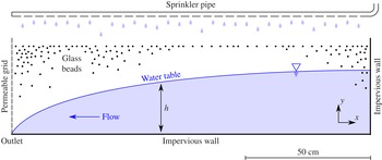
The simplest configuration of a free-surface aquifer consists of a homogeneous porous medium partly filled with water, the flow of which is confined to a vertical plane. We approximate this idealistic representation with a quasi-two-dimensional tank filled with glass beads of either 1 mm or 4 mm in diameter (figure 1). Using a Darcy column, we measure a conductivity
 $K$
of
 $0.97\pm 0.06\ \text{cm}\ \text{s}^{-1}$
for the 1 mm glass beads and
 $K=5.7\pm 1\ \text{cm}\ \text{s}^{-1}$
for the 4 mm glass beads. Two vertical glass plates (
 $143\ \text{cm}\times 40\ \text{cm}$
) separated by a 5 cm gap hold the glass beads between an impervious vertical wall (right-hand side), an impervious horizontal bottom and a permeable grid through which water can exit the experiment (left-hand side). The impervious wall corresponds to the drainage divide of a natural aquifer, whereas the outlet of the experiment is a rough representation of the drainage network.
Experimental aquifer. The water table (blue line) is submitted to atmospheric pressure. The aspect ratio is preserved.

Rainfall rate
 $R$
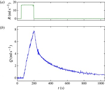
imposed on our laboratory aquifer (green line, a), and water discharge
 $Q$
exiting the experiment (blue line, b). Measurements are collected at 1 Hz, with a precision of approximately
 $0.1\ \text{g}\ \text{s}^{-1}$
. In this experimental run, the porous reservoir is made of 1 mm glass beads.

If the grid were in direct contact with air, surface tension would induce a pressure jump at the outlet. To avoid this inconvenience, we spread a soft plastic sheet over the outside of the grid. This device maintains a thin film of water at atmospheric pressure over the grid surface.
To simulate rainfall, a sprinkler pipe is held above the tank. A series of 31 holes spreads regularly along it, and distributes water evenly over the aquifer surface. Rainwater infiltrates vertically through the porous material until it reaches the bottom of the tank, where its accumulation forms a reservoir.
Above the reservoir, air connects the porous material to atmospheric pressure, thus maintaining the water it contains under capillary tension. For the 1 mm glass beads, this tension corresponds to approximately 1 cm of water. In what follows we neglect surface tension, and assume that the upper surface of the saturated reservoir is at atmospheric pressure. This free surface is referred to as the water table, of elevation
 $h$
(figure 1).
As the water table expands to accommodate more rainwater, the asymmetry of the boundary conditions causes it to curve towards the aquifer outlet. The resulting pressure field pushes the water out of the aquifer, generating a discharge
 $Q$
. The flow exiting the aquifer is collected in a bucket weighed every second with a precision of 0.1 g. The water discharge is then simply the derivative of the bucket weight with respect to time.
A typical experiment begins with an empty aquifer. We then switch on the rainfall and maintain its rate
 $R$
constant for a few tens of seconds (an electromagnetic flowmeter measures
 $R$
with a precision of 2 %). After a few seconds, the water discharge exiting the aquifer rises quickly, until the rainfall stops (figure 2). At this point, the discharge suddenly decreases, and then relaxes slowly towards zero.
In the experiment of figure 2, the water discharge increases approximately 40 s after the beginning of the rain. We observe a similar time lag in every experiment. We interpret it as the travel time of rainwater through the 40 cm of unsaturated porous medium that separates the aquifer’s surface from its bottom. A vertical velocity of approximately
 $1\ \text{cm}\ \text{s}^{-1}$
is indeed consistent with the measured conductivity of the saturated aquifer, although one could expect the porous medium to be less permeable when unsaturated.
3. Discharge increase
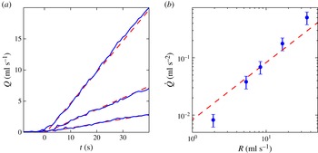
Once the rainwater has reached the bottom of the aquifer, the discharge at the experiment’s outlet appears to increase linearly with time (figure 3). This observation holds over the entire range of rainfall rates we were able to investigate (from
 $2.4\times 10^{-5}$
to
 $5.8\times 10^{-4}\ \text{m}\ \text{s}^{-1}$
). Naturally, if we maintain a constant rainfall for long enough, the water discharge will eventually saturate to equal the rainfall input. In what follows, we focus on the linear discharge increase that precedes this saturation.
(a) Increase of the water discharge just after the beginning of rainfall for various rainfall rates (solid blue lines,
 $R=36.7$
, 16.8 and
 $8.3\ \text{ml}\ \text{s}^{-1}$
from top to bottom). The curves are shifted horizontally so that time is zero at the beginning of the discharge increase. For each run, a linear increase is fitted to the data (dashed red lines). (b) Dependence of the discharge increase rate on the rainfall rate (blue dots). A linear relationship is fitted to the data for comparison (dashed red line). In this series of experiments, the porous reservoir is made of 4 mm glass beads.

A simple reasoning might explain the linear increase of the discharge during rainfall. Far from the outlet, the water table moves upwards in proportion to the water input, that is
 $Rt$
, and arguably so does the pressure in the reservoir. Assuming that the discharge is simply proportional to the pressure in the reservoir, we conclude that the discharge increase rate should be constant, and proportional to the rainfall rate
 $R$
.
We can measure the discharge increase rate
 $\dot{Q}$
by fitting a linear relation to the data, at the beginning of an experimental run (figure 3). On repeating this procedure for various rainfall rates, we find that the discharge increase rate is a growing function of the rainfall rate. This relationship, however, is not linear, and resembles a power law with an exponent larger than one. This finding contradicts the simple reasoning based on the linear pressure increase, thus suggesting that the discharge is not proportional to the elevation of the water table far from the outlet.
The nonlinear relation between discharge and pressure is a signature of a free-surface flow. Indeed, when the geometry of the flow is confined, Darcy’s law leads to a linear response of the aquifer. On the contrary, when the shape of the water table adjusts to the flow conditions, its dynamics influences the aquifer’s response to rainfall.
4. Dupuit–Boussinesq approximation
The Dupuit–Boussinesq approximation combines Darcy’s law with the shallow-water approximation to describe the groundwater flow in an unconfined aquifer (Boussinesq Reference Boussinesq1903; Polubarinova Kochina Reference Polubarinova Kochina1962). In a homogeneous and isotropic porous material, Darcy’s law reads
 $$\begin{eqnarray}\boldsymbol{v}=-K\,\boldsymbol{{\rm\nabla}}\left(\frac{p}{{\it\rho}g}+y\right),\end{eqnarray}$$
where
 $\boldsymbol{v}$
,
 $p$
,
 ${\it\rho}$
,
 $g$
and
 $y$
are the water flux, the pressure, the water density, the acceleration of gravity and the vertical coordinate respectively.
The applicability of the shallow-water approximation to our experiment depends on the aspect ratio of the flow. Based on direct observation through the side panels of the experiment, the elevation
 $h$
of the water table never exceeds 15 cm above the bottom of the aquifer; that is, about one tenth of its length. This suggests that the flow is almost horizontal which, through Darcy’s law, is equivalent to assuming that the pressure is hydrostatic. Accordingly, the total flux of water through a vertical line halving the aquifer reads
 $$\begin{eqnarray}q=-Kh\,\frac{\partial h}{\partial x}.\end{eqnarray}$$
Mass balance then leads straightforwardly to the one-dimensional Dupuit–Boussinesq equation:
 $$\begin{eqnarray}{\it\phi}\,\frac{\partial h}{\partial t}=\frac{K}{2}\,\frac{\partial ^{2}h^{2}}{\partial x^{2}}+R,\end{eqnarray}$$
where
 ${\it\phi}$
is the drainable porosity of the aquifer. The drainable porosity is the volume of water that gravity would extract from a saturated porous material, divided by the total volume of porous material. For our glass beads, we expect it to be 10 to 15 % lower than the material porosity (Johnson Reference Johnson1967). In what follows, we assimilate the drainable porosity to the total porosity. Based on the difference between the density of glass and the weight of a large collection of beads, we measure
 ${\it\phi}\approx 0.40$
for a random packing of 1 mm beads, and
 ${\it\phi}\approx 0.42$
for 4 mm beads.
As it is of second order in space, (4.3) must be supplemented with two boundary conditions. The impervious wall bounding the right-hand side of the aquifer imposes that the groundwater flux vanishes there (figure 1):
 $$\begin{eqnarray}\frac{\partial h}{\partial x}=0\quad \text{for }x=L,\end{eqnarray}$$
where
 $L$
is the length of the aquifer (we set the origin of the horizontal coordinate at the outlet).
The choice of a boundary condition at the outlet is less straightforward. If we neglect surface tension, we may assume that the water pressure tends towards the atmospheric pressure as the flow approaches the outlet. In the shallow-water framework, this approximation translates into
 $$\begin{eqnarray}h=0\quad \text{for }x=0.\end{eqnarray}$$
Unfortunately, this boundary condition creates a singularity at the outlet. Indeed, if
 $q_{o}$
is the flux of groundwater exiting the aquifer, then (4.2) implies that the water table elevation behaves like
 $$\begin{eqnarray}h\sim \sqrt{\frac{2\,q_{o}\,x}{K}}.\end{eqnarray}$$
Strictly speaking, this square root shape is incompatible with the shallow-water approximation, since the slope of the water table diverges near the outlet. Hereafter, we momentarily ignore this inconsistency and use the boundary condition (4.5) to solve the Dupuit–Boussinesq equation. We then discuss the possible consequences of this disregard.
5. Early response to rainfall
Our experiments suggest a power-law relationship between the discharge increase rate and the rainfall rate during the early stage of a rain event (figure 3). This is an incentive to look for the asymptotic behaviour of the Dupuit–Boussinesq equation at the beginning of rainfall.
Far from the outlet, we expect the groundwater flow to be insensitive to this boundary, and therefore the water table elevation should increase as
 $Rt/{\it\phi}$
, where the time
 $t$
is set to zero when rainwater reaches the bottom of the experiment. In contrast to the simple reasoning of § 3, we now propose a self-affine shape for the water table:
 $$\begin{eqnarray}h(x,t)=\frac{Rt}{{\it\phi}}\,H(X),\quad \text{where }X=\frac{{\it\phi}\,x}{t}\sqrt{\frac{2}{KR}}.\end{eqnarray}$$
The self-affine quantities
 $X$
and
 $H$
transform the Dupuit–Boussinesq equation into a parameterless ordinary differential equation:
 $$\begin{eqnarray}HH^{\prime \prime }+H^{\prime 2}+{\textstyle \frac{1}{2}}\left(XH^{\prime }-H+1\right)=0.\end{eqnarray}$$
The boundary condition at the outlet translates into
 $H(0)=0$
, while the steady rise of the water table far from the outlet formally reads
 $$\begin{eqnarray}\lim _{X\rightarrow +\infty }H=1.\end{eqnarray}$$
This boundary condition is valid as long as the impervious boundary is far from the outlet, compared with the characteristic length of the flow. Mathematically,
 $t\ll {\it\phi}\,L/\sqrt{KR}$
(for the experiment of figure 3,
 $t\ll 400\ \text{s}$
).
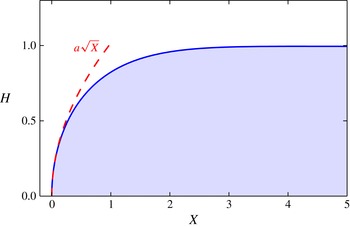
We are not aware of any analytical solution to the above problem, and therefore we approximate
 $H$
numerically (figure 4). Naturally, the affine transformation defined by (5.1) preserves the singularity of the water table near the outlet:
 $$\begin{eqnarray}H\sim a\,\sqrt{X},\end{eqnarray}$$
where
 $a$
is a constant adjusted to satisfy the far-field boundary condition (5.3). Using a numerical shooting method to do so, we find
 $a\approx 1.016$
.
Numerical solution of (5.2), corresponding to the self-affine shape of the water table during the early stage of a rain event (blue line). Its behaviour near the aquifer outlet is
 $a\,\sqrt{X}$
(red dashed line).

To the self-affine regime of the groundwater flow at early time corresponds the following water discharge, in dimensional form:
 $$\begin{eqnarray}Q(t)\sim a^{2}\,\frac{W}{{\it\phi}}\,\sqrt{\frac{K}{2}}\,R^{3/2}\,t,\end{eqnarray}$$
where
 $W$
is the width of the aquifer. The above expression is encouraging, as it features the linear time dependence of the discharge we observe in experiments. Furthermore, the prefactor of this relation includes the rainfall rate
 $R$
to a power larger than one, again in qualitative agreement with observations (figure 3).
To further compare this asymptotic regime with observation, we supplement the data of figure 3 with similar experiments involving a less permeable aquifer, made of 1 mm glass beads. Equation (5.5) suggests that the permeability
 $K$
be scaled out of the data:
 $$\begin{eqnarray}\frac{\dot{Q}\,{\it\phi}}{K^{2}W}\sim \frac{a^{2}}{\sqrt{2}}\left(\frac{R}{K}\right)^{3/2}.\end{eqnarray}$$
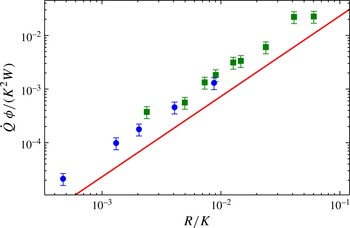
Indeed, when rescaled according to the above expression, the discharge increase rate and the rainfall rate from all experiments gather around the same relation, regardless of the permeability (figure 5). Fitting a power law through the data yields an exponent of
 $1.47\pm 0.01$
, in reasonable accordance with the
 ${\textstyle \frac{3}{2}}$
exponent of the asymptotic regime. Assuming that the asymptotic exponent is correct, the data are best fitted with a prefactor of
 $2.0\pm 0.1$
; that is, about three times the theoretical value of 0.73.
Dependence of the discharge increase rate with respect to the rainfall rate, for two series of experiments: 4 mm glass beads (blue dots) and 1 mm glass beads (green squares). The red line represents the asymptotic regime (5.6).

The asymptotic regime resulting in (5.6) explains the scaling of the discharge increase rate with both the rainfall rate and the conductivity, throughout the range of parameters we were able to explore experimentally. The overestimate of the drainable porosity could explain part of the mismatch between the theoretical prefactor and our measurements, though not all of it (§ 4).
This mismatch does not depend on the rainfall rate, or on the conductivity of the aquifer, which points to a geometrical effect. The breakdown of the Dupuit–Boussinesq approximation near the outlet indicates that the two-dimensionality of the flow plays a significant role there (§ 4). This could affect the boundary condition (4.5) and alter the prefactor of (5.5).
6. Drought flow
When the rain stops, the water discharge relaxes slowly towards zero. This drainage regime is referred to as the drought flow. In our experiment, groundwater exits the aquifer near its impervious bottom. In this configuration, the Dupuit–Boussinesq theory predicts that the discharge decreases as
 $1/t^{2}$
during the drought flow (Boussinesq Reference Boussinesq1903; Polubarinova Kochina Reference Polubarinova Kochina1962). We now compare this classical result with our observations.
In the absence of any source term (
 $R=0$
), the Dupuit–Boussinesq equation (4.3) has a self-similar solution:
 $$\begin{eqnarray}h(x,t)=\frac{L^{2}\,{\it\phi}}{Kt}\,H_{d}\left(\frac{x}{L}\right),\end{eqnarray}$$
where
 $L$
is the length of the aquifer, and the shape
 $H_{d}$
of the water table satisfies
 $$\begin{eqnarray}H_{d}\,H_{d}^{\prime \prime }+H_{d}^{\prime 2}+H_{d}=0,\end{eqnarray}$$
with two boundary conditions,
 $H_{d}^{\prime }(-1)=0$
and
 $H_{d}(0)=0$
. The discharge associated with this self-similar solution reads
 $$\begin{eqnarray}Q\sim a_{d}\,\frac{{\it\phi}^{2}\,WL^{3}}{Kt^{2}},\end{eqnarray}$$
where
 $a_{d}$
is a mathematical constant expressed in terms of the Euler gamma function
 ${\it\Gamma}$
(Brutsaert Reference Brutsaert2005):
 $$\begin{eqnarray}a_{d}=\frac{4}{3}\left(\frac{{\it\Gamma}(7/6)}{\sqrt{{\rm\pi}}\,{\it\Gamma}(2/3)}\right)^{3}\approx 0.693.\end{eqnarray}$$
By analogy with the linear heat equation, we expect most solutions of the Dupuit–Boussinesq equation to tend towards the self-similar solution
 $H_{d}$
at long times, regardless of the initial conditions. In contrast to the early stage of the discharge increase associated with a rain event, the drought flow depends on the length of the aquifer.
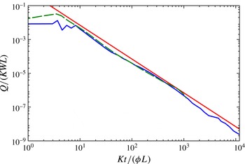
Our experimental aquifer conforms reasonably with the drought flow regime of the Dupuit–Boussinesq approximation (figure 6). After an appropriate rescaling, the relaxation of the water discharge appears to be independent of the aquifer permeability. Fitting a power law to the data after the transient (
 $Kt/({\it\phi}L)>10$
) yields an exponent of
 $-1.87\pm 0.03$
, comparable with the theoretical exponent. Assuming that this exponent is exactly
 $-2$
, the data are best fitted with a prefactor of
 $0.48\pm 0.2$
, again in reasonable agreement with the theoretical value of
 $a_{d}$
.
Evolution of the water discharge after rainfall has been switched off (blue solid line: 4 mm glass beads; green dashed line: 4 mm glass beads). The red line represents the asymptotic regime (6.3).

The slight mismatch between theory and observation is hardly distinguishable from the experimental noise, thus supporting the use of the Dupuit–Boussinesq approximation to interpret the drought flow of our experimental aquifer. Here again, the two-dimensionality of the flow and the overestimation of the drainable porosity might explain the discrepancy between the theoretical prefactor and observation (§ 5).
7. Conclusion
The experiment presented here supports the use of the Dupuit–Boussinesq approximation to describe the response of an aquifer to a rainfall event. In particular, it correctly predicts the increase of the groundwater discharge at the beginning of rainfall, and reveals an unexpected asymptotic behaviour: the discharge increase is proportional to the rainfall rate to the power of
 ${\textstyle \frac{3}{2}}$
.
If its validity extends to field situations, this strong dependence would induce a fast groundwater contribution to the discharge of rivers, especially under intense rainfall. Therefore, its consequences in terms of flood predictions deserve detailed scrutiny. An ideal field site to assess the contribution of this asymptotic regime would be dominated by groundwater hydrology, with negligible surface run-off. Under natural conditions though, various phenomena excluded from the present analysis, such as surface tension, heterogeneities of the aquifer and evapotranspiration, are likely to play a significant role.
However, even in a simplified laboratory experiment, the fast dynamics of a free-surface aquifer requires more investigation. Indeed, our experiment shows a slight mismatch between the numerical factors yielded by the Dupuit–Boussinesq approximation and measurements. We speculate that the two-dimensionality of the flow might come into play near the outlet, thus changing the effective boundary condition there.
More importantly, the geometry of our aquifer is most amenable to a shallow-water description, because the position of the outlet concentrates the flow near the impervious bottom. In a perhaps more realistic representation of a river, water would exit the aquifer at a finite elevation above the bottom, thus imposing an upwards flow below the outlet. This configuration certainly breaks the Dupuit–Boussinesq approximation, and its asymptotic regimes are still to be identified. This is the subject of present research.
Acknowledgements
We would like to thank H. Bouquerel, A. Veira and R. Vazquez-Paseiro for the conception of the experimental set-up. A. Daerr suggested the use of a plastic sheet to eliminate the pressure jump at the outlet of the experiment (§ 2). We are also grateful to F. Métivier, P. Davy, G. de Marsily, C. Narteau, A. P. Petroff, D. H. Rothman and J. W. Kirchner for fruitful discussions. O.D. is indebted to J. J. Grannel who introduced him to the problem. This work was inspired by a field campaign of the Observatoire de l’Eau et de l’Erosion aux Antilles.