1. Introduction
In recent years, there have been a number of models developed to try to ascertain future changes in mortality rates. Booth & Tickle (Reference Booth and Tickle2008) – who give a comprehensive overview of the history of mortality projections – identify three main approaches:
• explanation;
• expectation; and
• extrapolation.
Forecasting mortality by explanation involves building structural or epidemiological models to explain mortality from particular causes of death or known risk factors. This approach has the advantage that interactions between different factors and causes can be allowed for explicitly. This means that an element of subjectivity is required making statistical applications difficult although models for some diseases, such as the one for lung cancer developed by Alderson & Ashwood (Reference Alderson and Ashwood1985), have been developed.
There are a number of ways that expectation can be used to forecast mortality. A common approach, used by Pollard (Reference Pollard1987) and Olshansky (Reference Olshansky1988) involves defining a target life expectancy and then determining a path to that life expectancy. Such an approach allows expert opinion to be factored into the statistical process.
Extrapolation is the term given to forecasting future mortality based on past patterns. The most well-known of such approaches is the model developed by Lee & Carter (Reference Lee and Carter1992), “the Lee-Carter model”. However, earlier parametric approaches exist, including those developed by Heligman & Pollard (Reference Heligman and Pollard1980), Rogers & Planck (Reference Rogers and Planck1983) and others. The Lee-Carter model has itself seen many developments, such as the more robust treatment of errors by Brouhns et al. (Reference Brouhns, Denuit and Vermunt2002) and the addition of cohort effects by Renshaw & Haberman (Reference Renshaw and Haberman2006). There are also continuous time variants such as those developed by Milevsky & Promislow (Reference Milevsky and Promislow2001), Dahl (Reference Dahl2004), Dahl & Møller (Reference Dahl and Møller2005), Miltersen & Persson (Reference Miltersen and Persson2005), Biffis (Reference Biffis2005) and Schrager (Reference Schrager2006). The version I consider, however, has its roots in a discrete time model developed by Cairns et al. (Reference Cairns, Blake and Dowd2006). A more robust version of this model is given as model M5 in Cairns et al. (Reference Cairns, Blake, Dowd, Coughlan, Epstein, Ong and Balevich2009). This re-bases the age used to calculate the age-related component of the model, centring it around the average age of the data. Cairns et al. (Reference Cairns, Blake, Dowd, Coughlan, Epstein, Ong and Balevich2009) also describe a number of more complex versions of the original formulation. However, the simplicity of the original model, retained in model M5, is attractive and better allows the demonstration of the approach in this paper. I therefore use the M5 formulation, which I call the CBD model.
The CBD model is an innovative two-factor model. It assumes that each of the two parameters follows a random walk with drift, the rate of drift being constant and changes in the parameters being correlated. This approach is well-suited for the pricing of mortality-related derivatives with a term of a few years; however, when considering the very long-term, it becomes clear that the patterns for these two factors do not necessarily resemble a random walk with drift process; for most periods each of the factors can be modelled as a random fluctuation around a trend, the trend changing periodically.
This is not the first research to question the use of a random walk with a single rate of drift as the appropriate method of mortality projection. Booth et al. (Reference Booth, Maindonald and Smith2002) find that the level of drift for Australian data is not constant, and allow for this by fitting their model only for the period where a linear trend in mortality is apparent. Using the same dataset, De Jong & Tickle (Reference De Jong and Tickle2006) allow for varying rates of drift over time, and suggest improvements such as the addition of an autoregressive process to the parameters used; however, like Booth et al. (Reference Booth, Maindonald and Smith2002), mortality rates are assumed to follow a random walk.
The CBD model describes the logit of the initial mortality rate with a slope term and an intercept term, allowing for the number of deaths to follow a Poisson distribution. Future stochastic simulations are then obtained by projecting these two terms as following correlated random walks. In other words:

where qx ,y is the initial mortality rate for a life aged x in year y (that is, the proportion of lives aged exactly x at the start of year y expected to die before the end of year y);  is the average of the ages x used in the analysis; k 1,y is the intercept term in year y; k 2,y is the slope term in year y; and ey is an error term. The parameters k 1,y and k 2,y are members of sets described by k 1 = {k 1,y : y = 1…Y} and k 2 = {k 2,y : y = 1…Y}, and k 1 and k 2 are equivalent to the state variables described in the CBD model as kappa 1 and kappa 2 respectively.
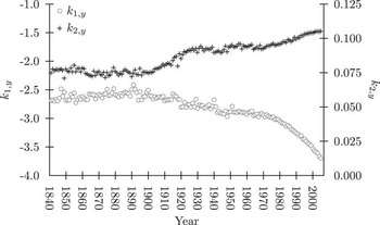
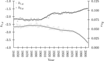
The CBD model is calibrated using data for England and Wales males from age 60 to 89 over the period 1961 to 2002. However, this is a relatively short time scale which has seen a generally steady pattern of improvements in life expectancy. It is not reasonable to expect this constancy to continue indefinitely into the future, something which can be seen by considering past mortality rate improvements over a longer period. One way of appreciating these past changes is to fit the CBD model over a larger dataset, covering the period from 1841 to 2005, still using England and Wales males age 60 to 89. Here, clear patterns can be seen in k 1,y and k 2,y, as shown in Figure 1. The data used for these calculations is obtained from the Human Mortality Database (2008). Figure 1 suggests that both k 1,y and k 2,y exhibit variation around a trend rather than following random walks. They also suggest that these trends change suddenly and definitely, that changes in the trend for k 1,y and k 2,y tend to happen at the same time, and that there is strong negative correlation between the direction of these trend changes.
k 1,y and k 2,y for the CBD Model, 1841-2005 (Source: Human Mortality Database (2008), Author's Calculations)

These sudden changes in the trend are what one would expect, considering changes that have happened over the last 160 years or so. Cutler et al. (Reference Cutler, Deaton and Lleras-Muney2006) describe three phases of change in mortality rates. From the mid eighteenth century to the mid nineteenth century, they see mortality rates falling as a result of improved nutrition and economic growth; in the late nineteenth and early twentieth centuries, improvement is seen as a result of clean water, better treatment of effluent and better health information, all of which became necessary as a result of urbanisation; and the 1930's onwards is characterised as the decade of big medicine with immunisation, antibiotics, and ever-increasing medical technology. Another phenomenon that continues to have a major effect on mortality rates is the effect of the reduction in smoking in the last quarter of the twentieth century, as described by Humble Wilson (Reference Humble and Wilson2008).
The negative correlation is also understandable. From Equation 1 it can be seen that at time t, k 1,y represents the level of the logit of mortality, and k 2,y the extent to which the logit of mortality varies with age. The second variable therefore reflects changes in the relative levels of mortality at different ages, but the first variable determines the underlying change in mortality around which the relative changes are based.
The organisation of this paper is, then, as follows. First, I consider ways in which change-points in the trend can be determined. I then fit trends to different sections of the data. Within each of these sections, I then consider whether the observations are trend- or difference-stationary. Next, I propose an approach for projection mortality rates based on this structure, and finally I show the results of some of these projections.
2. Determining the Change-Points in the Trend
Looking at Figure 1, it is clear that there are breaks in the trend for both k 1 and k 2. However, it is not necessarily clear exactly where these breaks occur, and whether any changes are significant enough to be considered changes in trend.
One way of investigating possible change-points is to fit lines to sections of k 1 and k 2 and to calculate the Durbin-Watson (DW) statistic, using the test designed by Durbin & Watson (Reference Durbin and Watson1950, Reference Durbin and Watson1951). The test is described in detail in the appendix. Under the null hypothesis that a fitted line covers data within a single trend, the DW statistic should show no evidence of significant serial correlation between subsequent values of k 1,y or k 2,y. Consider, however, a line fitted to a series of observations from k 1,y. Suppose that these observations cover two distinct periods, the average rate of change in k 1,y being lower in the second period than the first. Fitting a single line to this series of observations would result in earliest and latest observations lying below the line with the middle observations lying above the line. This would lead to the DW statistic showing significant positive serial correlation in these variables, suggesting that the null hypothesis could be rejected and that there was evidence for a break in the trend. This approach is not exact, but gives some clues as to where breaks might occur. In particular, the period around which significant positive serial correlation appears suggests the time at which a structural break occurs.
The methodology used for the above approach is to fit a series of lines starting in each year y where y = 1841 to 2003 (so using at least three years of data to calculate the DW statistic). For each year, lines are fitted for periods p where p = 3 to 2005−y. This means that for 1841 there are 163 lines covering periods from three years to 165 years, whilst for 2003 there is only one line covering the three-year period from 2003 to 2005. This approach can point to broad areas where changes in trend might occur. Consider, for example, the results from applying the DW test to k 1,y for y = 1875 and p = 10 – in other words, for the years k 1,1875 to k 1,1884 inclusive. If the value of the DW statistic does not suggest any significant positive serial correlation, then no structural break is indicated in that period. However, if subsequent tests for p = 11, 12, 13… and so on suggest significant positive serial correlation, then this indicates that there is a structural break in the series k 1,y in around 1885. If the first significant positive serial correlation for the data series starting y=1876 occurs when p = 10, and for the data series starting y = 1877 occurs when p = 9 – in both cases, when data from 1885 have been added – then this strengthens the impression that there is a structural break around this point, particularly if the positive serial correlation becomes more significant with additional observations.
However, the DW test was not designed with this use in mind, so cannot give the statistical significance of any change in the trend. It can therefore only give an indication of the approximate time at which a structural break might occur. To get more accurate results, techniques specifically designed to detect structural breaks are needed.
3. Fitting a Model
Having identified potential breakpoints both visually and using the DW test, the results are verified using more exact approaches. The broad approach used to fit lines to k 1,y and k 2,y is a weighted least squares approach. This is necessary because of the heteroskedasticity present in both k 1,y and k 2,y. In particular, the variance decreases substantially over time. There are several possible causes for this. The first is simply that the quality of data is likely to have improved over the period of observation. However, as life expectancies have increased, so have the number of lives over age 60. This leads to less stochastic variation in the mortality rates calculated, and thus less variation in the estimates of k 1,y and k 2,y from year to year. A third possibility is that improved understanding and treatment of infectious diseases together with improved air and water quality reduced the incidence of various epidemics that also led to significant falls in the year-to-year variation in mortality.
The weights used are the reciprocals of the variances for the seven years centred on the observation in question. The weights for the first three observations are set equal to the weight for the fourth observation; the weights for the last three observations are set equal to the weight for the fourth from last observation.
I first consider k 1. Let the final year of a trend (and the first year of the next) within k 1 be identified as bk 1,n (k 1) where n(k1)=1 … N(k1)−1. This means that the number of break points is N(k1)−1 and the number of lines is N(k1). Each line is expressed as a constant, αk 1,n (k 1) plus a slope, βk 1,n (k 1), the latter being multiplied by the year. This means that the estimate of k 1,y is described as follows:
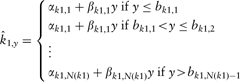
Similarly, the estimate of k 2,y is described as follows:
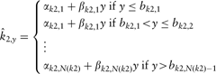
It can also be said that:

and

where ε k 1,y and ε k 2,y are residuals. Initially, N(k1) is set equal to N(k2). Furthermore, all bk 1,n (k 1) are set equal to bk 2,n (k 2). This second point seems sensible, since a visual inspection of k 1,y and k 2,y suggests that changes in trends occur at about the same time in one as in the other, although there are perhaps some instances when a significant change occurs in only one series. There is also a rationale for expecting changes in k 1,y and k 2,y to occur at the same time, since a change in both determines the age around which relative changes in mortality pivot. This is investigated below.
When fitting the lines, all potential changes in trend are considered initially. This means not only considering all potential instances where the trend may change, but also a range of years for each break. The lines are then fitted by minimising the sum of squared errors subject to the restriction that:

and:

for n(k1) = 1… N(k1)−1 and n(k2) = 1… N(k2)−1.
The first test I carry out is a Chow test, as described by Chow (Reference Chow1960), applying it to each consecutive pair of sections of the data. This test is described in detail in the appendix, and it is modified here using the weighting described above in order to remove heteroskedasticity. Under the Chow test, the null hypothesis is that αk 1,n (k 1) = αk 1,n (k 1)+1 and βk 1,n (k 1) = βk 1,n (k 1)+1 for consecutive groups of data within k 1, the same being true for k 2. The Chow test is helpful in examining structural breaks since it considers not the extent to which individual observations represent a change from an established trend, but rather the extent to which two groups of variables display different patterns.
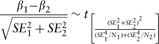
I also consider the statistical significance of the change in the slope between potential breaks in the trend. The restrictions in Equations 6 and 7 effectively mean that the slope parameters are optimised subject to restrictions on the level parameters. This means that looking at the difference between successive slope parameters can help to identify where any change in slope is not statistically significant. This is done by dividing the change in the slope by the joint standard error, this being calculated assuming unequal sample sizes and unequal variances in each sample. The calculation approach is described in the appendix. The null hypothesis here is that there is no change in slope.
I also consider the DW statistic for the various sections. If separate trends are combined, then this may be highlighted by significant positive serial correlation, suggesting that a change in trend has been missed.
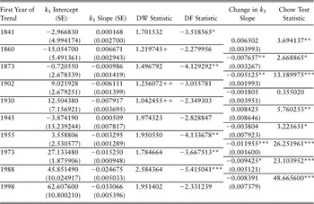
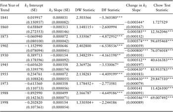
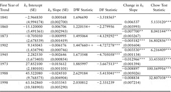
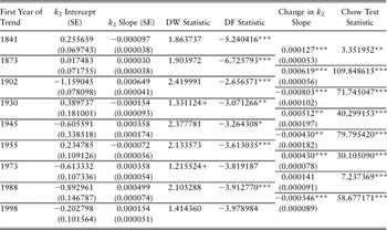
The exact year chosen for each break is the year that maximises the Chow Test statistics. These results are shown in Tables 1 for k 1 and Table 2 for k 2. These tables also include the Dickey-Fuller (DF) statistic, the use of which is discussed in more detail later. This test is also described in detail in the appendix.
Parameters for fitted values of k 1.

Significance level: ***1%; **5%; *10%.
Serial correlation: ++ evidence of significant positive serial correlation (statistic< dL);+evidence of possible positive serial correlation (dL< statistic< dU).
Parameters for fitted values of k 2.

Significance level: ***1%; **5%; *10%.
Serial correlation: ++ evidence of significant positive serial correlation (statistic< dL);+evidence of possible positive serial correlation (dL< statistic< dU).
Looking first at k 1, a number of break points appear to be less than convincing, suggesting the need for further investigation; however, the only break point not strongly suggested by the Chow Tests in k 2 is the first.
In order to determine which of the potential breaks should be ignored, the model is re-run a number of times assuming either that each break occurs or is ignored. If ignoring a break results in the DW test suggesting significant positive serial correlation, then the break is generally reinstated; if, however, there is no significant positive serial correlation, then unless the Chow or change-in-trend test strongly suggests a structural break the potential break is ignored. The resulting breakpoints are as shown in Tables 3 and 4.
Revised parameters for fitted values of k 1.

Significance level: ***1%; **5%; *10%.
Serial correlation: ++ evidence of significant positive serial correlation (statistic< dL);+evidence of possible positive serial correlation (dL< statistic< dU).
Revised parameters for fitted values of k 2.

Significance level: ***1%; **5%; *10%.
Serial correlation: ++ evidence of significant positive serial correlation (statistic< dL);+evidence of possible positive serial correlation (dL < statistic < dU).
Again, looking first at k 1, the Chow test statistic strongly suggests breaks at all the points remaining. The change-in-trend test suggests changes in most of these instances. However, combining any sections into a single series results in significant positive serial correlation.
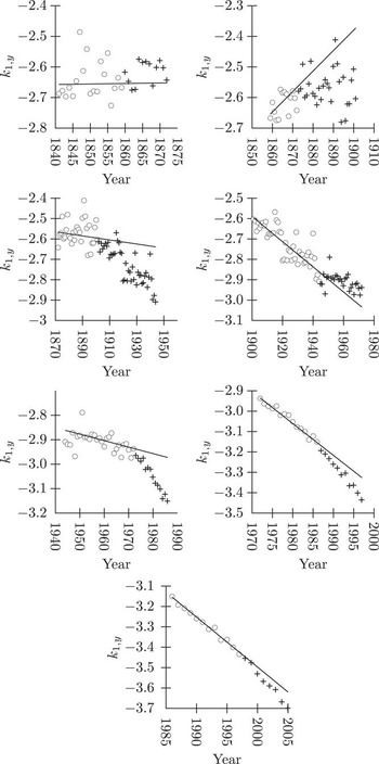
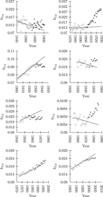
One of the combinations carried out to arrive at Table 3 does result in positive serial correlation. This is for the series starting in 1902 and ending in 1944. However, looking at the results in Figure 2 – and more clearly shown in the right-hand chart in the second row of Figure 3 – suggests that this is more likely to be a result of random clustering than two separate trends having been combined.
Lines Fitted to k 1,y and k 2,y for the CBD Model, 1841–2005 (Source: Human Mortality Database (2008), Author's Calculations)

Changes in Trend for k 1,y Slope – Post-Change Observations vs Pre-Change Fitted Line (Source: Human Mortality Database (2008), Author's Calculations)

The single change lost in k 2 is less controversial. The Chow test suggests that no further changes are needed, and the DW statistics do not suggest that any trends have been combined incorrectly.
It is tempting to look through the history books in an attempt to identify events that might have resulted in changes in parameters. However, such an approach invites behavioural biases. Having said this, we can see a change in the parameters from the mid 1860s to mid 1870s, around the time that the London sewerage system was opened, improving sanitation in the capital. This was also just after various nursing initiatives had been implemented in the UK. Mortality improvements also appear to slow in two periods that coincide with economic depressions, one from the mid 1870s to the end of the nineteenth century, and another from 1929 to the early 1940s. A change is also seen in the years following the founding of the NHS, and again when the impact of changing smoking habits fed through to older age mortality in the final quarter of the twentieth century.
One reported statistic has not been discussed in detail: the DF statistic. Under the null hypothesis of the test designed by Dickey & Fuller (Reference Dickey and Fuller1979) the time series under investigation follows a random walk with drift – in other words, it has a unit root. The alternative hypothesis is that the time series consists of random deviations from a trend. For k 1, the DF test suggests that the data follows random deviations around a trend in six out of eight periods; for k 2, the figure is seven out of nine periods. In most case, the level of significance is 1%.
Ideally, the DF statistic would be calculated for the whole period. However, since the calculation of the statistic involves regression against a time trend and it has already been shown that this trend changes over time, such a test is not straightforward. In particular, changes in the direction of the trend of either the level or the slope parameter will result in unreliable results. The change-of-trend issue is also why this test is considered now, rather than before the investigations into the break-points in the trend. One possible modification to the DF test in the presence of a changing trend is to substitute the linear time trend with a series constructed from the slope parameters. If the slope in year y for parameter k 1 is yβk 1, then this replacement trend for k 1 can be calculated as yzk 1 = y βk 1 + y −1βk 1, where 1zk 1 = 1βk 1. Note that yβk 1, the slope parameter in year y, should not be confused with βk 1,N (k 1), the slope parameter for all y falling in trend N(k1). Similarly, the replacement trend for k 2 can be calculated as yzk 2 = y βk 2 + y −1βk 2, where 1zk 2 = 1βk 2. Using this approach, the null hypothesis for the data series as a whole is rejected at the 1% level of significance, with the test statistics for k 1 and k 2 being −10.32 and −13.06 respectively. This provides strong evidence that each parameter follows a trend-stationary process, albeit with a trend that changes periodically.
Figure 2 shows how the fitted lines described in Table 3 and Table 4 relate to the parameters shown in Figure 1. However, the scale of these diagrams is such that it is difficult to see the extent to which the trend does actually change. Figure 3 and Figure 4 are therefore given. These show the values of k 1,y and k 2,y for each consecutive pairs of trends, as described in Table 3 and Table 4. They also show the fitted line for the first trend extended to the period covered by the second trend. This is intended to show the extent to which a change in trend occurs. In most cases the change is marked; in others it is less definitive but nonetheless apparent.
Changes in Trend for k 2,y Slope – Post-Change Observations vs Pre-Change Fitted Line (Source: Human Mortality Database (2008), Author's Calculations)

4. A Projection Approach
Having fitted a model to the data, I next look at an approach to projecting mortality rates. The first stage here is to consider how the parameters behave in the historical data.
Since Equations 6 and 7 mean that the changes in αk 1,n (k 1) and αk 2,n (k 2) are defined by the changes in βk 1,n (k 1) and βk 2,n (k 2), it is only the latter that we need to consider when looking at changes of the trends in k 1,y and k 2,y. The trend in k 1,y changes 7 times out of a possible 164 times, a probability of 0.042683; the trend in k 2,y changes 8 times in the same period, a probability of 0.048780. However, βk 1,n (k 1) and βk 2,n (k 2) change together only six of these times. This means that:
• the probability of only βk 1,n (k 1) changing is 1 in 164, or 0.006098;
• the probability of only βk 2,n (k 2) changing is 2 in 164, or 0.012195;
• the probability of both βk 1,n (k 1) and βk 2,n (k 2) changing is 6 in 164, or 0.036585.
These changes can therefore be modelled by simulating a uniform random variable, 0 ≤ Δβ < 1, such that:
• if 0 ≤ Δβ < 0.006098 then βk 1,n (k 1) only changes;
• if 0.006098 ≤ Δβ < 0.042683 then βk 1,n (k 1) and βk 2,n (k 2) change (since 0.042683−0.006098 = 0.036585);
• if 0.042683 ≤ Δβ < 0.054878 then βk 2,n (k 2) only changes (since 0.054878–0.042683 = 0.012195; and
• if Δβ ≥ 0.054878 then neither βk 1,n (k 1) nor βk 2,n (k 2) change (since 0.006098 + 0.012195 + 0.036585 = 0.054878, or 9/164.
The next stage is to look at the variation in βk 1,n (k 1) and βk 2,n (k 2) when they change. One approach would be to consider the root mean square (RMS) of the deviation of each variable from its previous value and use this to define the volatility. This would mean essentially assuming that the expectation was for the current trends in k 1,y and k 2,y to continue indefinitely, with each being as likely to accelerate as to decelerate. The alternative is to use the standard deviation. This would give a lower level of volatility, but would require an assumption that changes in k 1,y and k 2,y would be expected to accelerate or decelerate (depending on whether the average was positive or negative). This latter view seems unrealistic, as it suggests that both k 1,y and k 2,y would eventually tend towards positive or negative infinity, leading to biologically unrealistic mortality rates. I therefore use an approach based on the RMS, described above. I also calculate a measure of correlation between βk 1,n (k 1) and βk 2,n (k 2) when both change using a similar approach, calculating a measure of covariance based on deviations from zero rather than from the mean, then dividing the result by the RMS of βk 1,n (k 1) and βk 2,n (k 2). The correlation calculated by this method – effectively an “RMS correlation coefficient” – is −0.301142, compared with the “true” correlation coefficient – calculated as the actual covariance of βk 1,n (k 1) and βk 2,n (k 2) divided by the standard deviation of each – of 0.380513. As discussed above, there is a good reason to use the RMS instead of the standard deviation when measuring volatility. This reason – that using the standard deviation would lead to unrealistic mortality rates – also applies to the measure of correlation. This suggests that the RMS correlation coefficient is more appropriate than the true one. This view is strengthened by the observation that the two lines in Figure 2 diverge in a reasonably consistent fashion over the full period of investigation. Divergence and convergence are both consistent with a negative correlation coefficient; a positive coefficient would suggest that the two series should move in broadly the same direction.
When both βk 1,n (k 1) and βk 2,n (k 2) change, the RMS of the former is 0.008406 (compared with a standard deviation of 0.005597) and of the latter is 0.000405 (compared with a standard deviation of 0.000352). However, the RMS for βk 1,n (k 1) using all changes is 0.015998 (compared with a standard deviation of 0.013719), and for βk 2,n (k 2) is 0.000332 (compared with a standard deviation of 0.000287). An F-test suggests that the volatility differs for k 1,y, but only at the 10% level; there is no significant difference for βk 2,n (k 2). However, the small number of observations means that it is difficult to draw any strong conclusions. In the analysis below, I use the same volatility when only one variable changes or both change.
Finally, given that the data is to be modelled assuming random volatility around a trend, the nature of this volatility needs to be investigated. Analysis of the standard deviation of the errors, ε k 1,y and ε k 2,y, shows that the volatility decreases successively in each period, but there is a particularly large and sustained fall for both βk 1,n (k 1) and βk 2,n (k 2) in 1973. I therefore assume that the volatility around the trend is given by the volatility calculated using data since this date, 0.012098 for ε k 1,y and 0.000627 for ε k 2,y.
Having determined the parameters for the projection of mortality, I then project mortality forward stochastically. This is done by projecting values for βk 1,n (k 1) and βk 2,n (k 2). A uniform random variable taking values between 0 and 1 is generated in each period. The value of the random variable determines whether either or both of βk 1,n (k 1) and βk 2,n (k 2) change, as described earlier. If either variable changes, then another random variable is generated with a mean of zero and a standard deviation taken as the RMS of past changes in βk 1,n (k 1) or βk 2,n (k 2). If both change, then the random variables are generated assuming an RMS correlation as given above. The correlated random variables are generated using Cholesky decomposition, as described in Wilmott (Reference Wilmott2006) and elsewhere. Each change is independent of any previous changes. If βk 1,n (k 1) and/or βk 2,n (k 2) change, then αk 1,n (k 1) and/or αk 2,n (k 2) also change as described in Equations 6 and 7 – in other words, they change in such a way as to avoid there being a discontinuity at the point that the trend changes. These values are used to calculate projected values of  and
 , extrapolating the relationship in Equations 2 and 3.
As discussed earlier,  and
 are only estimators, and there is uncertainty in these estimates. This is given by ε k 1,y and ε k 2,y, as described in Equations 4 and 5. The projected results for
 and
 are therefore modified by the addition of further random variables which are independent and normally distributed with means of zero and standard deviations of 0.012098 and 0.000627 respectively, reflecting the volatility in recent years.
5. Projection Results
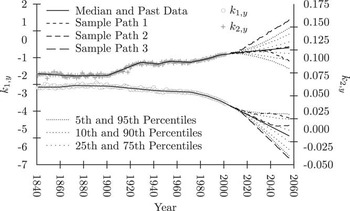
Using the method and data above, I carry out 1,000 simulations of k 1,y and k 2,y. The median projection is shown with confidence intervals for the simulations in Figure 5. Three sample paths are also shown. These are the first three simulations from k 1,y and k 2,y, meaning that the two sets of sample paths relate to the same simulations for each variable. The sample paths show not only how wide the range of outcomes could be, but also the extent to which extreme trends in one direction for one variable do tend to be offset by extreme trends in the opposite direction for the other.
Lines Fitted to k 1,y and k 2,y for the CBD Model, 1841–2005 (Source: Human Mortality Database (2008), Author's Calculations)
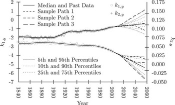
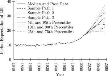
I then use these results to calculate the period life expectancy of a 65-year old male for the fifty year period from 2006 to 2056. Whilst the model is calibrated using data from ages 60 to 89, rates are projected up to age 120 using the same model, with the mortality rate for 121 being fixed at 1. Age 65 is used to allow comparison with published figures for the CBD model. I show the results in Figure 6. Displayed are the median and various percentile limits, together with three sample paths. The sample paths are calculated from values of k 1,y and k 2,y shown in Figure 5.
Historical and Projected Period Life Expectancy for 65 Year Old Males, England and Wales, 1841–2056 (Source: Human Mortality Database (2008), Author's Calculations)

This shows that the range of results in early years is relatively narrow, but uncertainty does grow rapidly. To illustrate, the 90% confidence interval – calculated as the difference between the 5th and the 95th centiles – for period life expectancy in 2056 is 18.7 years (37.6 years for the 95th centile less 18.9 years for the 5th centile). Dowd et al. (Reference Dowd, Blake and Cairns2008) perform similar calculations to arrive at cohort (rather than period) life expectancies for 65 year old males for the same projection period (2006 to 2056), using a version of the CBD model that allows for cohort effects. If parameter uncertainty is ignored, the 90% confidence interval in 2056 spans 3.6 years; even if parameter uncertainty is allowed for, the range rises to only 7.6 years. In other words, this trend-change model suggests more than twice as much uncertainty as the cohort-adjusted CBD model with parameter uncertainty over a fifty-year time horizon, and the shape of the funnel suggests that the difference in uncertainty continues to increase.
The confidence intervals are reminiscent of those achieved through the p-spline approach described by Eilers & Marx (Reference Eilers and Marx1996). However, unlike the p-spline approach, the methodology described in this paper uses the full data history to produce projected values. It is also more suited than the p-spline approach for the production of stochastic mortality projections which can be combined with the outputs from stochastic asset models.
Although the distribution of the number and size of trend changes reflects the statistically significant changes in the historical data, some of those changes are more easily identifiable visually than others. It is interesting to consider the implications of using only the more obvious changes, and these implications are that the trends will change less frequently but more severely than in the projections above. Consider, for example, a scenario where there are only two changes of trend in k 1,y, in 1873 and 1973 whilst there are three changes of trend in k 2,y occurring in 1902, 1930 and 1973. This means that there is still a 1 in 164 chance of a change in only βk 1,n (k 1), and still a 2 in 164 chance of a change in only βk 2,n (k 2), but that the chance of a simultaneous change in both has been reduced from 6 in 164 to 1 in 164. Simultaneously the RMS for βk 1,n (k 1) increases from 0.015998 to 0.018413 whilst the RMS for βk 2,n (k 2) rises from 0.000332 to 0.001196. Since the one joint change – in 1973 – is in the opposite direction for the two variables, an RMS correlation of −1 is assumed. Under this set of assumptions, the 90% confidence interval for the period expectation of life at age 65 falls from 18.7 to 11.5 years. Whilst this is still almost half as big again as the CBD parameter uncertainty estimate, it is markedly smaller than the results discussed earlier. This indicates that both the number of changes and the size of those changes has a large impact on the level of uncertainty present in mortality projections. It also emphasises the importance of using statistical tests to try to spot changes in trend rather than relying on visual inspection.
6. Conclusion
If a two parameter model of the type described by Cairns et al. (Reference Cairns, Blake and Dowd2006) is used to model mortality, then the parameters follow clear trends that change periodically. The changes in the parameters frequently occur at the same time and are negatively correlated. Within each trend, the parameters do seem to be random fluctuations around a trend rather than random walks with drift. The random fluctuations can be explained as changes in the underlying rate of mortality from year to year due to environmental factors such as the harsh winters or influenza outbreaks. However, these changes are overlaid onto longer term trends whose changes can be explained in terms of structural developments such as industrialisation, changes in sanitation or the introduction of antibiotics.
Modelling mortality into the future using the approach described in this paper suggests a much greater degree of uncertainty than that implied by random walks with drift, although the level of uncertainty is heavily dependent on the number of changes in trend discovered, and the distribution of these changes.
This has important consequences for risk management and pricing, in particular when considering longer term insurance products such as annuities. The greater uncertainty over mortality rates in the distant future suggests that higher reserves are needed than those suggested by a random walk with drift approach inherent in the original CBD model. The need for higher reserves should also be reflected in pricing.
Another consequence of this pattern of changing mortality rates is that a low level of volatility in mortality rates over a given period should not be interpreted as a fall in the level of risk – a change in the trend rate of mortality improvement could occur at any point in time, potentially causing a large change in predicted mortality rates.
The potential application of this trend-change approach is not confined to CBD-type models. In particular, it could also be applied to the model proposed by Lee & Carter (Reference Lee and Carter1992) as well as those based on this approach. In this way, it would act as an additional extension to those suggested by De Jong & Tickle (Reference De Jong and Tickle2006). As discussed earlier, their paper has several suggestions for dealing with unstable trends, including taking care over the choice of parameterisation period and adding an autoregressive element to the description of the parameters. However, allowing a random change in the trend rates of mortality improvement combined with volatility around the trend rate would give greater long-term variation in mortality rates than any of the approaches suggested by De Jong & Tickle (Reference De Jong and Tickle2006).
The approach described above is not the only way of allowing for the change-in-trend feature seen in the data. For example, instead of changing the trend, the time scale could be altered whilst the trend was kept constant, as described by Hyndman & Booth (Reference Hyndman and Booth2008). However, whilst this approach has a number of attractive theoretical properties it is not immediately clear how the significance of changes in trend could be determined in such a model.
The model described in this paper does itself have limitations. For example, only ages 60 to 89 are modelled. The more complex mortality structure for younger ages, and the possibility that trends at these ages could change due to different factors than older ages, presents a number of modelling challenges. Even if the model were to be used only for over 60 s, the assumption that the logit-linear relationship between age and mortality extends above age 90 is strong as Cairns et al. (Reference Cairns, Blake, Dowd, Coughlan, Epstein, Ong and Balevich2009) mention. The model also describes the mortality only for males. Without extension, a similar – but independent – model would need to be devised for females, although as suggested by Li & Lee (Reference Li and Lee2005) there are a number of common influences that should be taken into account. The cohort effect, as described by Wilmoth (Reference Wilmoth1990) is also ignored, although the model could be extended to take this into account.
It is also important to recognise that if this model is used to calculate the uncertainty in the expectation of life for a given population then the characteristics of that population should be considered. Uncertainty over the underlying nature of the population means that the uncertainty over the forecasts will be higher. Furthermore, the fact that the population is finite will also mean that additional uncertainty will arise due to random variation in the actual times of death.
However, these limitations do not affect the insights given by the model described in this paper. In particular, the approach I propose suggests that there should be much greater allowance for uncertainty in mortality rates in the distant future, and that a failure to allow for this uncertainty could be costly.
A. Statistical Tests
A.1. The Durbin-Watson Test
The Durbin-Watson test is a test designed to detect serial correlation in the residuals or error terms from a regression. If εt is the error term from a regression at time y where y = 1, 2, … Y, then the Durbin-Watson statistic, d, is calculated as:
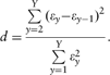
There is an implicit assumption that the error terms are normally distributed and that they have a constant variance. If there is no serial correlation, then the result of this calculation is d = 2. The null hypothesis is therefore that d does not differ significantly from 2. The Durbin-Watson tables, used to determine the significance of any deviation from 2, have two values for any given level of confidence. The lower one, dL, is the value below which positive serial correlation exists at the table's level of confidence, whilst the upper one, dU is the value above which there is no evidence of significant serial correlation. Between dL and dU lies an area of uncertainty, where the test is said to be inconclusive.
Both dL and dU are lower than 2. However, the test can be used to detect both positive and negative serial correlation. Therefore, if d < dL, then there is evidence that there is significant positive serial correlation, whilst if (4−d) < dL there is evidence of significant negative serial correlation. If dU < d < 4−dU, there is no evidence of significant serial correlation. However, if dL < d < dU or dL < 4−d < dU, the test is inconclusive.
A.2. The Chow Test
The Chow Test is used to test for structural breaks in time series. To carry out the test, a model is fitted to a set of observations. The data are then divided into two sets and the same model is fitted to each separately. The test statistic is then given as:

where SSR 1, SSR 2 and SSRAll are the sums of squared residuals from the first section of data, the second section of data and the combined dataset respectively. The number of variables is given by υ, and the numbers of observations in the first and second groups of data are given by N 1 and N 2.
The null hypothesis is that there is no significant difference between the fit of the models when fitted to two sections and to the full dataset. The test statistic has an F-distribution with υ and N 1 + N 2−2υ degrees of freedom.
The Chow Test is carried out under the assumption that the error terms are normally distributed with a constant variance.
A.3. The Dickey-Fuller Test
The Dickey-Fuller test is designed to test for the presence of a unit root, that is, whether a dataset is difference- or trend-stationary. A stationary process is often characterised as “white noise”. A difference-stationary process is one where the data do not themselves follow a stationary process, but where difference between subsequent observations does. If, after differencing, the stationary process is around a non-zero value, then the original dataset is said to follow a random walk with drift. A trend-stationary process is one where the data do follow a stationary process around a deterministic trend.
Under the null hypothesis of the test designed by Dickey & Fuller (Reference Dickey and Fuller1979) the time series under investigation follows a random walk with drift – in other words, it has a unit root. The alternative hypothesis is that the time series consists of random deviations from a trend.
To carry out the test, the following equation is fitted:

where ky is the observation of k at time y, α 0, α 1 and α 2 are parameters and ε y is an error term. The test of a unit root is a test of whether α 2 is significantly different from zero. If it is, then the null hypothesis can be rejected. This part of the process involves using a t-test, that is, dividing the coefficient of α 2 by its standard error from the regression equation. However, the t-distribution cannot be used to test for the significance of α 2 and a specific Dickey-Fuller table must be used instead.
A.4. Testing for a Change in Trend with a t-Test
In relation to a regression equation, the standard t test is carried out to determine whether a coefficient is significantly different from zero. This involves dividing the coefficient β by its standard error SE, the resulting statistic having a t distribution with N−v degrees of freedom, N being the number of observations and v being the number of explanatory variables. In other words:

However, if the significance of the difference between two coefficients is of interest, a revised standard error is needed. Consider two sets of observations with the measurements relating to each denoted by the subscripts 1 and 2. If the variances between two samples are unequal, then the standard error for a test involving both sets of observations is calculated as  . The number of degrees of freedom is also different, and is approximately equal to
 . This means that the difference between two coefficients can be tested as: