2. Related literature

With the onset of the rational expectations revolution, the existence of multiple equilibria in macroeconomic models emerged as the focus of several studies. For instance, Sargent and Wallace (Reference Sargent and Wallace1975) conclude that under rational expectations, the price level becomes undetermined in the IS-LM model if the government pegs the nominal interest rate. In a similar vein, Obstfeld and Rogoff (Reference Obstfeld and Rogoff1983) show that the equilibrium path of the price level is not uniquely determined in a model with infinitely lived maximizing households with perfect foresight. Also, Sargent (Reference Sargent1987, Chapter 8) provides an overview of several results on the indeterminacy of the composition of the public debt. In turn, Woodford (Reference Woodford1994) studies the equilibrium indeterminacy issue in an economy with cash and credit goods.

Three aspects of this problem warrant further comment. First, the indeterminacy may arise in many distinct forms. For instance, only the price level is affected by it in Sargent and Wallace (Reference Sargent and Wallace1975) and Obstfeld and Rogoff (Reference Obstfeld and Rogoff1983), while it also impacts real variables in Woodford (Reference Woodford1994). Second, the equilibrium multiplicity became even more ubiquitous when, as in Chari and Kehoe (Reference Chari and Kehoe1990), macroeconomists started applying the tools of the theory of infinitely repeated games. Third, Atkeson et al. (Reference Atkeson, Chari and Kehoe2010) warn against the adoption of the approach that they call unsophisticated implementation when trying to design a macroeconomic policy that uniquely implements an outcome. As they point out, this approach fails to verify whether the proposed policy also constitutes an equilibrium after a deviation from the equilibrium path. Since I focus on subgame-perfect equilibrium, this is not a point of concern here.

The theoretical notion that the introduction of an inflation-targeting policy may contribute to the coordination of the expectations and actions of economic agents is often found in the literature. For instance, Bernanke et al. (Reference Bernanke, Laubach, Mishkin and Posen1999, p. 11) state that the inflation-targeting system “provides a focus for the expectations of financial markets and the general public,” while Walsh (Reference Walsh2009) argues that this type of policy “can align the public’s expectations of current and future target rates with the actual goals of the central bank” (p. 200) and may anchor “the public’s beliefs about future inflation” (p. 201).

The following picture emerges from the previous paragraphs: while equilibrium multiplicity is widely recognized in the broader macroeconomics literature, the conventional wisdom found in its inflation-targeting branch posits that this regime should help agents to coordinate their expectations and actions. However, from a theoretical point of view, it is unclear how an inflation-targeting policy can achieve this. For instance, Smith (Reference Smith1994) shows that multiple competitive equilibria can exist under inflation targeting in an overlapping generations model, and Adão et al. (Reference Adão, Correia and Teles2011) conclude that the same result holds in a cash-in-advance model.

At this stage, it is necessary to clarify a matter. It has been argued that, in the context of a New Keynesian model, a socially optimal policy can be uniquely implemented if the central bank follows an interest-rate rule that prescribes a sufficiently strong response to output and inflation shocks (for further details, see Galí, Reference Galí2015, Chapter 4, Section 3.1). Although related, this is not the problem addressed in this paper. The focus here is on whether and how an inflation-targeting policy, by itself, can lessen the problem of equilibrium multiplicity. Moreover, as discussed in a broader context by Atkeson et al. (Reference Atkeson, Chari and Kehoe2010), it is far from clear that such an interest-rate rule can be a rational choice for an optimizing central bank.

Interestingly, the empirical evidence seems to be consistent with the aforementioned conventional wisdom. Indeed, Svensson (Reference Svensson and Svensson2011, p. 1247) argues that “There is relatively robust empirical evidence that an explicit numerical target for inflation anchors and stabilizes inflation expectations.” Capistrán and Ramos-Francia (Reference Capistrán and Ramos-Francia2010, p. 115) find that “the dispersion of long-run inflation expectations appears to be smaller under IT [inflation-targeting] regimes than in non-IT ones.” Gürkaynak et al. (Reference Gürkaynak, Levin and Swanson2010, p. 1210) state that their findings “support the view that a transparent and credible inflation target helps to anchor the private sector’s perceptions of the distribution of long-run inflation outcomes.” At the micro level, Bambe et al. (Reference Bambe, Combes, Kaba and Minea2024, p. 3) conclude that “inflation targeting significantly increases firm performance” and that this finding appears to be “related with the capacity of the inflation targeting framework to reduce macroeconomic instability.”

The results presented in this paper provide a theoretical reconciliation, within the framework of an infinitely repeated game, of the conventional wisdom on the effects of an inflation-targeting policy with the problem of multiple equilibria in macroeconomic models. Moreover, if one assumes that a lessening of the degree of equilibrium multiplicity helps agents to coordinate their expectations and actions, then such a reconciliation is consistent with the empirical evidence.

The seminal papers of Kydland and Prescott (Reference Kydland and Prescott1977), Calvo (Reference Calvo1978), and Barro and Gordon (Reference Barro and Gordon1983a and Reference Barro and Gordon1983b) establish that, in the absence of a commitment mechanism, even a benevolent central banker can implement an inflation rate higher than the socially optimal one. Rogoff (Reference Rogoff1985) shows that this problem can be solved by placing an agent whose payoff, when compared to the relevant social welfare function, places a heavier weight on achieving low inflation relative to the weight placed on attaining low unemployment. One can interpret the fixed penalty as an instrument for achieving Rogoff’s solution, even if the central banker is not sufficiently averse to inflation.

Although none of them addresses the exact problem studied here, this paper is very closely related to Gersbach and Hahn (Reference Gersbach and Hahn2006), Libich (Reference Libich2009), and Araujo et al. (Reference Araujo, Berriel and Santos2016). They all use variants of the Barro-Gordon model. Moreover, each of them adopts a hypothesis similar or identical to the fixed-penalty assumption of this paper. Below, I discuss each of them separately.

Gersbach and Hahn (Reference Gersbach and Hahn2006) compare the monetary-targeting regime with the inflation-targeting one in a single-period game with asymmetric information. In their model, there is a demand shock that is not observed by the public but that may or may not be observed by the central bank. The general public does not know whether or not the central bank observed the shock. The authors conclude that it is easier for the central bank to commit to a low rate of inflation under the inflation-targeting regime than under the monetary-targeting regime, since the former policy is more directly related to future inflation. Concerning the fixed penalty, its precise arrangement depends on the regime. Under monetary targeting, the central bank does not incur the payoff loss whenever the money supply is equal to the announced target. Under inflation targeting, the penalty is not assessed if the target rate of inflation is met or the money supply is equal to the value that an uninformed central bank that wants to achieve the target rate would select.Footnote ⁵

Libich (Reference Libich2009) considers a finitely repeated game with complete information. He assumes that the general public faces a fixed payoff loss every period in which the long-run (i.e., average over time) inflation rate is not equal to the socially optimal inflation rate. The frequency with which the central bank can adjust the target rate of inflation is exogenous. According to him, the longer the adjustment interval, the more explicit the inflation target. On the other hand, the general public can select the frequency with which its expectations will be updated. Since there is a cost of doing so (which depends on the update frequency), this player may optimally choose not to update in some periods. Libich says that the public expectations are anchored if (i) the general public chooses not to update its expectations at every period and (ii) the average over time of its period-inflation expectation is equal to the socially optimal inflation rate. Next, he says that an explicit inflation target has an anchoring effect in equilibrium if (iii) the public expectations are anchored and (iv) the frequency with which the general public updates is related in a nondecreasing fashion to the frequency with which the target is changed. In line with the results presented in this paper, Libich shows that there is a unique subgame-perfect equilibrium if the aforementioned fixed payoff loss is sufficiently large. Moreover, this equilibrium displays the anchoring effect.

Araujo et al. (Reference Araujo, Berriel and Santos2016) adopt a single-period game in which the central bank faces a fixed penalty identical to the one in this paper. They study how the size of the penalty impacts the central bank’s ability to implement low targets. Initially, they carry out this analysis in a full-information environment. In a result identical to the one obtained in this paper, they conclude that depending on the values of the target and of the penalty, there may be: (i) a unique equilibrium in which the outcome is the Barro-Gordon discretionary inflation rate; (ii) a unique equilibrium in which the outcome is the target rate; or (iii) two equilibria, characterized by the two outcomes just described. Next, they assume that the general public is composed of a continuum of players who do not have perfect information about the value of the penalty faced by the central bank. These players receive public and private signals about the variable in question. Araujo, Berriel, and Santos show that, under some conditions on the preferences of the central bank, the target rate, the Barro-Gordon discretionary inflation rate, and the precision of the public signal relative to the private signal, there is a unique monotone perfect Bayesian equilibrium for every public signal. They also conclude that the lowest target rate consistent with equilibrium uniqueness decreases as public information becomes noisier.Footnote ⁶ This last result is in line with the findings of Jia and Wu (Reference Jia and Wu2023), who argue that ambiguous communication may enhance the credibility of the central bank.

I conclude this section by pointing out that this paper is also related to the literature on contracts for central bankers started by Persson and Tabellini (Reference Persson and Tabellini1993) and Walsh (Reference Walsh1995). Those authors, as well as Mishkin and Westelius (Reference Mishkin and Westelius2008), argue that an inflation-contingent compensation scheme can have effects similar to an inflation-targeting policy. Consistent with this view, I show in Section 9 that introducing the penalty is equivalent to assuming that the central banker receives a performance bonus whenever the actual inflation rate is equal to the target. Hence, this paper can be seen as a study of the effects of a specific type of compensation scheme for the central banker.

3. Preliminaries: The stage game

In this section I present and analyze the stage game underlying the infinitely repeated game that is the focus of this paper. To facilitate the exposition, I first discuss a version of the stage game without inflation targeting. This version is based on the single-period inflation bias models of Kydland and Prescott (Reference Kydland and Prescott1977) and Barro and Gordon (Reference Barro and Gordon1983a and Reference Barro and Gordon1983b). In a second step, I modify the game to incorporate the inflation-targeting regime.

3.1 A game without inflation targeting

There are two players in the game: the central bank (player $b$ ) and the general public (player $p$ ). Players move simultaneously. Agent $p$ selects a value $\pi ^{e}$ for the expected inflation rate. Its choice must lie in the set $\Pi =[0,\pi _{\max }]$ , where $\pi _{\max }$ is a positive number large enough so that it is never reached in any of the equilibria discussed in this paper. Player $b$ selects a value $\pi \in \Pi$ for the actual inflation rate. Given those choices, the value $y\in \mathbb{R}$ of the natural logarithm of GDP is determined according to the Phillips curve

\begin{equation*} y=\bar {y}+\alpha (\pi -\pi ^{e})\text{,}\end{equation*}

where $\bar {y}$ is the natural logarithm of the natural rate of output and $\alpha$ is a positive parameter. The payoff of the general public is given by

\begin{equation*} V(\pi ^{e},\pi )=-(\pi -\pi ^{e})^{2}\text{.}\end{equation*}

The quadratic loss function

(1) \begin{equation} w(y,\pi )=-\{\gamma \pi ^{2}+[y-(1+\mu )\bar {y}]^{2}\}\text{,} \end{equation}

where $\gamma \gt 0$ and $\mu \gt 0$ , is the payoff of the central bank.Footnote ⁷

As usual, one can use the Phillips curve to express the payoff of player $b$ as a function of $\pi ^{e}$ and $\pi$ . Define the function $W$ so that $W(\pi ^{e},\pi )=w(\bar {y}+\alpha (\pi -\pi ^{e}),\pi )$ . Hence,

(2) \begin{equation} W(\pi ^{e},\pi )=-\{\gamma \pi ^{2}+[\alpha (\pi -\pi ^{e})-\mu \bar {y}]^{2}\}\text{.} \end{equation}

From now on, I use the function $W$ to describe the central bank’s payoff. This player’s problem is

(3) \begin{equation} \max _{\pi \in \Pi }W(\pi ^{e},\pi )\text{,} \end{equation}

while player $p$ solves

(4) \begin{equation} \max _{\pi ^{e}\in \Pi }V(\pi ^{e},\pi )\text{.} \end{equation}

A Nash equilibrium for this game is a vector $(\hat {\pi }^{e},\hat {\pi })$ such that: (i) given $\hat {\pi }^{e}$ , $\hat {\pi }$ solves the problem of player $b$ ; and (ii) given $\hat {\pi }$ , $\hat {\pi }^{e}$ solves the problem of player $p$ .

The game has a unique Nash equilibrium. Denote the partial derivatives $\partial W/\partial \pi ^{e}$ and $\partial W/\partial \pi$ by, respectively, $W_{1}$ and $W_{2}$ . For a fixed $\pi ^{e}$ , the function $W(\pi ^{e},\cdot )$ is strictly concave. Therefore, the solution of (3) is characterized by

(5) \begin{equation} W_{2}(\pi ^{e},f(\pi ^{e}))=0\text{,} \end{equation}

where $f$ is the best response function of $b$ . It is a simple exercise to show that

(6) \begin{equation} f(\pi ^{e})=\frac {\alpha ^{2}}{\gamma +\alpha ^{2}}\pi ^{e}+\frac {\alpha \mu }{\gamma +\alpha ^{2}}\bar {y}\text{.} \end{equation}

Optimality by player $p$ requires $\pi ^{e}=\pi$ . Thus, $\hat {\pi }^{e}=\hat {\pi }=f(\hat {\pi })$ . As a consequence,

(7) \begin{equation} \hat {\pi }=\frac {\alpha \mu }{\gamma }\bar {y}\text{.} \end{equation}

It should be pointed out that $\hat {\pi }$ is the unique fixed point of $f$ .

3.2 The stage game with inflation targeting

In this subsection I carry out two tasks. First, I modify the previous game to incorporate the inflation-targeting regime. Second, I characterize the equilibrium set of the resulting new game. Each of those tasks is carried out in a separate subsection.

3.2.1 Introducing inflation targeting

I assume that an outside agent (for instance, the legislature) carries out the task of modifying the game. This agent implements two changes. First, it publicly announces that player $b$ (the central bank) has to pursue a target $\pi ^{\ast }\in (0,\hat {\pi })$ for the inflation rate.Footnote ⁸ Second, it assesses a fixed penalty on player $b$ whenever the actual inflation rate differs from the target $\pi ^{\ast }$ . Whenever the penalty is applied, the central bank faces a payoff loss equal to $C\gt 0$ .Footnote ⁹ Formally, define the indicator function $I$ so that

\begin{align*} I(\pi )= \begin{cases} 1, & \text{if} \ \pi \neq \pi ^{\ast }\\[3pt] 0, & \text{if} \ \pi =\pi ^{\ast } \end{cases} \text{.} \end{align*}

The function $U$ , which is given by

(8) \begin{equation} U(\pi ^{e},\pi )=W(\pi ^{e},\pi )-I(\pi )C\text{,} \end{equation}

is the central bank’s payoff. Section 9 contains a detailed analysis of the fixed-penalty assumption. As discussed there, the value of $C$ can be interpreted as a concise metric of the strength of the institutions in charge of supervising the central bank.

3.2.2 Equilibrium

The problem of player $p$ (the general public) is still given by (4), while player $b$ (the central bank) solves

(9) \begin{equation} \underset {\pi \in \Pi }{\max }\text{ }U(\pi ^{e},\pi )\text{.} \end{equation}

A stage Nash equilibrium is a vector $(\pi ^{e},\pi )$ such that: (i) given $\pi ^{e}$ , $\pi$ solves the problem of player $b$ ; and (ii) given $\pi$ , $\pi ^{e}$ solves the problem of player $p$ .

I now turn to the task of characterizing the equilibrium set of the stage game. This requires solving problem (9). Since $U$ is discontinuous at $\pi =\pi ^{\ast }$ , this cannot be done using solely the standard tools. Fortunately, there is a simple procedure that works out in this context: compare the values of $U(\pi ^{e},f(\pi ^{e}))$ and $U(\pi ^{e},\pi ^{\ast })$ and select the argument $f(\pi ^{e})$ or $\pi ^{\ast }$ that yields the higher payoff. Lemma 1 formalizes this discussion.Footnote ¹⁰

The equilibrium set depends on the size of the penalty. Thus, the next step consists of attributing precise meanings to the notions of small, large and intermediate values of $C$ . Define the parameters $k_{1}$ and $k_{2}$ according to

(10) \begin{align} k_{1}=W(\pi ^{\ast },f(\pi ^{\ast }))-W(\pi ^{\ast },\pi ^{\ast }) \end{align}

and

(11) \begin{align} k_{2}=W(\hat {\pi },f(\hat {\pi }))-W(\hat {\pi },\pi ^{\ast })\text{.} \end{align}

Since $f(\pi ^{e})$ uniquely maximizes $W(\pi ^{e},\cdot )$ and $\pi ^{\ast }$ is different from $f(\pi ^{\ast })$ and $f(\hat {\pi })$ , both $k_{1}$ and $k_{2}$ are positive. It is shown in Lemma 3 that $k_{1}\lt k_{2}$ .Footnote ¹¹ Therefore, it is possible to say that the penalty is small when $C\lt k_{1}$ , large when $C\gt k_{2}$ , and intermediate when $C\in \lbrack k_{1},k_{2}]$ .

Now, suppose that the penalty is small. In this case, the inflation-targeting regime is not relevant, and the only stage Nash equilibrium must be $(\hat {\pi },\hat {\pi }),$ which is the one identified in the game without inflation targeting. On the other hand, if $C$ is large, then the central bank will play $\pi ^{\ast }$ regardless of whether $\pi ^{e}=\hat {\pi }$ or $\pi ^{e}=\pi ^{\ast }$ . In anticipation of this, the general public will optimally play $\pi ^{\ast }$ . Hence, in this case the only stage Nash equilibrium is $(\pi ^{\ast },\pi ^{\ast })$ . If $C$ takes an intermediate value, then there are exactly two stage Nash equilibria, $(\hat {\pi },\hat {\pi })$ and $(\pi ^{\ast },\pi ^{\ast })$ . Proposition 4 formalizes this intuitive description of the equilibrium set.

4. The infinitely repeated game

In this part of the paper I start the study of the game constituted by the infinite repetition of the stage game of the previous section. In Subsection 4.1, I carry out some basic tasks, such as setting up some notation and presenting a suitable equilibrium concept. In Subsection 4.2, I specify the conditions that characterize the set of all equilibrium outcomes that can be supported by trigger strategies that specify reversion to one of the Nash equilibria of the stage game.

4.1 Structure and equilibrium definition

Denote a vector $(\pi _{t}^{e},\pi _{t})$ of date- $t$ actions by $x_{t}$ , while $\rho$ and $\delta$ are the respective discount factors of players $p$ (the general public) and $b$ (the central bank). As usual, these two parameters belong to the interval $(0,1)$ .Footnote ¹² Given a sequence $\{x_{t}\}_{t=0}^{\infty }$ of actions, the payoffs of $p$ and $b$ from date $t$ onwards are given, respectively, by

(12) \begin{equation} \sum _{r=t}^{\infty }\rho ^{r-t}V(\pi _{r}^{e},\pi _{r}) \end{equation}

and

(13) \begin{equation} \sum _{r=t}^{\infty }\delta ^{r-t}U(\pi _{r}^{e},\pi _{r})\text{.} \end{equation}

Let $h^{t}$ be a history $(x_{0},x_{1},\ldots ,x_{t})$ of actions. At the beginning of each date $t$ , both players know the history $h^{t-1}$ . The general public implements an action $\pi _{t}^{e}\in \Pi$ , while the central bank implements an action $\pi _{t}\in \Pi$ . Denote these choices by $s_{t}(h^{t-1})$ and $\sigma _{t}(h^{t-1})$ . Thus, a strategy for $p$ is a sequence $s=\{s_{t}\}_{t=0}^{\infty }$ , while a strategy for $b$ is a sequence $\sigma =\{\sigma _{t}\}_{t=0}^{\infty }$ . At each date $t$ , given the history $h^{t-1}$ and the strategy $\sigma$ of player $b$ , $p$ selects a continuation sequence $\{s_{r}\}_{r=t}^{\infty }$ to maximize (12). This player takes into consideration that the actions of $b$ evolve according to $\pi _{r}=\sigma _{r}(h^{r-1})$ . In similar fashion, given $h^{t-1}$ , $s$ , and the rule $\pi _{r}^{e}=s_{r}(h^{r-1})$ , $b$ selects a continuation sequence $\{\sigma _{r}\}_{r=t}^{\infty }$ to maximize (13).Footnote ¹³

A subgame-perfect equilibrium for the infinitely repeated game is a pair of strategies $(s,\sigma )$ such that, at every date $t$ and for every history $h^{t-1}$ , $\{s_{r}\}_{r=t}^{\infty }$ solves the problem of the general public and $\{\sigma _{r}\}_{r=t}^{\infty }$ solves the problem of the central bank. A subgame-perfect equilibrium outcome is a sequence $\{x_{t}\}_{t=0}^{\infty }$ with the property that there is an equilibrium $(s,\sigma )$ that satisfies $\pi _{t}^{e}=s_{t}(x_{0},x_{1},\ldots ,x_{t-1})$ and $\pi _{t}=\sigma _{t}(x_{0},x_{1},\ldots ,x_{t-1})$ .

Since the subgame-perfect equilibrium is the only type of equilibrium of the infinitely repeated game considered, hereafter I will drop the qualification “subgame-perfect” to avoid tedious repetition. Moreover, as mentioned in the Introduction, I will use shorthand expressions such as trigger equilibrium and trigger equilibrium outcome to refer to an equilibrium supported by trigger strategies and the resulting outcome.

4.2 A set of equilibrium outcomes

In this subsection, I describe the set of all trigger equilibrium outcomes. I denote this set by $\mathcal{T}(C)$ , where the $\mathcal{T}$ stands for trigger and the $C$ is included to emphasize the set’s dependence on the value of the penalty.

Given the dependence of the set of stage equilibria on the value of $C$ , it is necessary to split the analysis into two cases. Suppose that $C\gt k_{2}$ . In this case, $(\pi ^{\ast },\pi ^{\ast })$ is the unique stage equilibrium. Thus, the characterizing conditions are

(14) \begin{equation} \pi _{t}=\pi _{t}^{e} \end{equation}

and

(15) \begin{equation} \sum _{r=t}^{\infty }\delta ^{r-t}U(\pi _{r}^{e},\pi _{r})\geq \max _{\pi \in \Pi }U(\pi _{t}^{e},\pi )+\delta \frac {U(\pi ^{\ast },\pi ^{\ast })}{1-\delta }\text{.} \end{equation}

Observe that (14) is the optimality condition for the general public, while (15) ensures the central bank has no incentive to deviate from a candidate sequence $\{x_{t}\}_{t=0}^{\infty }$ .

Suppose now that $C\leq k_{2}$ . If $C$ happens to be smaller than $k_{1}$ , then $(\hat {\pi },\hat {\pi })$ is the unique stage Nash equilibrium. Hence, the characterizing conditions are (14) and

(16) \begin{equation} \sum _{r=t}^{\infty }\delta ^{r-t}U(\pi _{r}^{e},\pi _{r})\geq \max _{\pi \in \Pi }U(\pi _{t}^{e},\pi )+\delta \frac {U(\hat {\pi },\hat {\pi })}{1-\delta }\text{.} \end{equation}

On the other hand, if $C\in \lbrack k_{1},k_{2}]$ , two stage Nash equilibria exist: $(\hat {\pi },\hat {\pi })$ and $(\pi ^{\ast },\pi ^{\ast })$ . While the general public is indifferent between $(\hat {\pi },\hat {\pi })$ and $(\pi ^{\ast },\pi ^{\ast }),$ the central bank prefers $(\pi ^{\ast },\pi ^{\ast })$ because $U(\pi ^{\ast },\pi ^{\ast })\gt U(\hat {\pi },\hat {\pi })$ . Therefore, to characterize all equilibrium outcomes that can be supported by reverting to a stage Nash equilibrium, one must use the more severe reversion point $(\hat {\pi },\hat {\pi })$ . As a consequence, the characterizing conditions are, again, (14) and (16).

Summing up, if $C\gt k_{2}$ , then $\mathcal{T}(C)$ is characterized (14) and (15); if $C\leq k_{2}$ , then the characterizing conditions are (14) and (16). This discussion is formalized in Proposition 6.

5. Sustaining the target rate of inflation as a trigger equilibrium outcome

Questions such as “Do we really need an explicit inflation-targeting system to achieve the target rate of inflation?” and “If so, how large does the penalty have to be?” are central to this paper. These are precisely the issues addressed in this section.

Let $X^{\ast }$ denote the sequence $\{x_{t}\}_{t=0}^{\infty }$ in which $x_{t}=(\pi ^{\ast },\pi ^{\ast })$ for all $t$ . Technically, the questions posed in the previous paragraph are equivalent to asking for which values of $C$ the sequence $X^{\ast }$ belongs to $\mathcal{T}(C)$ . I analyze this problem below.

I break the analysis into two cases: (i) $C\geq k_{1}$ and (ii) $C\lt k_{1}$ . In the former, $(\pi ^{\ast },\pi ^{\ast })$ is a stage Nash equilibrium. Since $X^{\ast }$ is simply the infinite repetition of $(\pi ^{\ast },\pi ^{\ast })$ , it must belong to $\mathcal{T}(C)$ .

Consider now Case (ii). In this context, $\mathcal{T}(C)$ is characterized by conditions (14) and (16). Clearly, $X^{\ast }$ satisfies (14). Regarding (16), $X^{\ast }$ satisfies this inequality if and only if

(17) \begin{equation} \frac {U(\pi ^{\ast },\pi ^{\ast })}{1-\delta }\geq \max _{\pi \in \Pi }U(\pi ^{\ast },\pi )+\delta \frac {U(\hat {\pi },\hat {\pi })}{1-\delta }\text{.} \end{equation}

Since $C\lt k_{1}$ , one can show that

\begin{equation*} \max _{\pi \in \Pi }U(\pi ^{\ast },\pi )=U(\pi ^{\ast },f(\pi ^{\ast }))\text{.}\end{equation*}

Combine this equality with the definition of the payoff function $U$ to conclude that (17) is equivalent to

(18) \begin{equation} \frac {W(\pi ^{\ast },\pi ^{\ast })}{1-\delta }\geq W(\pi ^{\ast },f(\pi ^{\ast }))-C+\delta \frac {W(\hat {\pi },\hat {\pi })-C}{1-\delta }\text{.} \end{equation}

Next, define the parameter $k_{0}$ so that

\begin{equation*} k_{0}=(1-\delta )k_{1}-\delta \lbrack W(\pi ^{\ast },\pi ^{\ast })-W(\hat {\pi },\hat {\pi })]\text{.}\end{equation*}

A little algebra establishes that (18) holds if and only if $C\geq k_{0}$ .Footnote ¹⁴

Recapituling, the condition $X^{\ast }\in \mathcal{T}(C)$ is satisfied unconditionally in Case (i), while in Case (ii) it holds if and only if $C\geq k_{0}$ . Therefore, $X^{\ast }\in \mathcal{T}(C)$ if and only if $C\geq k_{0}$ . This result is formally established in Proposition 7.

Note that it may happen that $k_{0}$ is nonpositive; for instance, this is surely the case for $\delta$ sufficiently close to $1$ . This has some implications for the implementation of $X^{\ast }$ . If $k_{0}\leq 0$ , then $X^{\ast }$ is an equilibrium outcome regardless of the value of the penalty $C$ (including the limiting case of $C=0$ ). On the other hand, in an economy with a positive $k_{0}$ , a positive penalty is a necessary condition for $X^{\ast }$ to be a trigger equilibrium outcome.

6. The impact of penalty changes on the set of trigger equilibrium outcomes

In this section I carry out an exercise that can be understood as a type of comparative statics. More specifically, I assess how changes in the penalty $C$ impact the set of trigger equilibrium outcomes $\mathcal{T}(C)$ . This analysis will show how a larger penalty can contribute to the implementation of the target rate of inflation.

The aforementioned exercise entails asking what happens to $\mathcal{T}(C)$ as a consequence of an increase in $C$ . Answering this question requires assessing how such a variation affects the trigger equilibrium outcome characterizing conditions (14), (15), and (16). Since the first of them does not depend on the penalty, the problem reduces to analyzing what happens to the latter two. Care must be taken to account for the fact that, depending on whether $C\leq k_{2}$ or $C\gt k_{2}$ , the relevant condition is either (16) or (15). For this reason, I break the analysis into the three cases below.

1. (i) Both the initial and the final value of the penalty are smaller than or equal to $k_{2}$ .

2. (ii) The initial value of the penalty is equal to $k_{2}$ , while the final value is larger.

3. (iii) Both the initial and the final values of the penalty are larger than $k_{2}$ .

Observe that in both (i) and (iii) the value of the penalty is restricted to one of the two possible ranges, while in (ii) the value of the penalty is moving from one range to the other.Footnote ¹⁵

Before proceeding with the analysis of each case, it is necessary to introduce some additional notation. Let $\mathbb{X}$ be the set of all sequences in $\Pi \times \Pi$ . A generic element of $\mathbb{X}$ is denoted by $X$ , while $\hat {X}$ is the sequence in which $x_{t}=(\hat {\pi },\hat {\pi })$ for all $t$ . The subset of $\mathbb{X}$ containing all sequences with the property that $\pi _{t}=\pi ^{\ast }$ for some $t$ is denoted by $\mathbb{X}^{\ast }$ , while $\mathbb{\tilde {X}}^{\ast }$ is the subset of $\mathbb{X}$ containing all sequences such that $\pi _{t}\neq \pi ^{\ast }$ for every $t$ (i.e., the complement of $\mathbb{X}^{\ast }$ with respect to $\mathbb{X}$ ). I also have to clarify a minor point concerning the usage of the symbols $\subseteq$ and $\subset$ . The latter requires the inclusion to be a proper one, while the former allows the two sets under analysis to be equal.

For case (i), suppose that $C\lt k_{2}$ . Hence, the reverting sequence is $\hat {X}$ . Now, let $X$ be a trigger equilibrium outcome in which $\pi _{r}\neq \pi ^{\ast }$ for every date $r$ . That is, 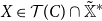$X\in \mathcal{T}(C)\cap \mathbb{\tilde {X}}^{\ast }$ . Consider a generic date $t$ . For dates later than $t$ , the value of $C$ is irrelevant to the central bank when comparing the payoffs of $X$ and $\hat {X}$ , since the penalty will be assessed at every date under both sequences. However, by deviating to $\pi ^{\ast }$ on date $t$ , the central bank can avoid the penalty on that date. Therefore, the larger the value of $C$ , the greater the incentive for the central bank to deviate from $X$ by implementing $\pi ^{\ast }$ on date $t$ . Thus, as $C$ increases (but does not become larger than  $k_{2}$ ), sequences belonging to $\mathbb{\tilde {X}}^{\ast }$ tend to be excluded from $\mathcal{T}(C)$ . This discussion is formalized in Proposition 8. Consequently, provided that the new value of the penalty does not exceed $k_{2}$ , if an increase in the penalty adds a sequence $X$ to the set $\mathcal{T}(C)$ , then this sequence must belong to $\mathbb{X}^{\ast }$ (i.e., $X$ must hit $\pi ^{\ast }$ at least once).

As discussed in the previous section, $X^{\ast }$ is a trigger equilibrium outcome if and only if $C\geq k_{0}$ . Consequently, if $X^{\ast }$ is a trigger equilibrium outcome for a given penalty, then it remains so for any larger penalty. At a first glance, it may appear that this result can be extended to any sequence belonging to $\mathbb{X}^{\ast }$ . However, an additional condition is required. Indeed, consider two penalties $C_{1}$ and $C_{2}$ such that $C_{1}\lt C_{2}\leq k_{2}$ . Now, let $X\neq X^{\ast }$ be a trigger equilibrium outcome in which, for $C=$ $C_{1}$ , the target $\pi ^{\ast }$ is hit on some date. That is, $X\in \mathcal{T}(C_{1})\cap \mathbb{X}^{\ast }$ . Let $t$ be any date on which $\pi _{t}\neq \pi ^{\ast }$ . It may happen that an increase in $C$ induces the central bank to deviate to $\pi ^{\ast }$ on date $t$ to avoid incurring a higher penalty. However, if on future dates $X$ repeatedly hits $\pi ^{\ast }$ , such a deviation may not be an optimal action for the central bank. Indeed, consider the inequality

(19) \begin{equation} \sum _{r=t+1}^{\infty }\delta ^{r-t}[1-I(\pi _{r})]\geq I(\pi _{t})\text{.} \end{equation}

The sum on the left-hand side is simply a discounted count of the number of times that $X$ hits the target $\pi ^{\ast }$ after date $t$ . Since $I(\pi ^{\ast })=0$ , this inequality will surely hold if $\pi _{t}=\pi ^{\ast }$ . If $\pi _{t}\neq \pi ^{\ast }$ , the sum will have to be equal to or greater than $1$ for the condition to hold. As shown in Proposition 10, if $X$ belongs to $\mathcal{T}(C_{1})$ and satisfies (19) for every $t$ , then $X$ belongs to $\mathcal{T}(C_{2})$ . Therefore, provided that the inequality $C\leq k_{2}$ is not violated, if a sequence is removed from the set of trigger equilibrium outcomes as a consequence of an increase in the penalty, then it must be the case that $X$ does not hit $\pi ^{\ast }$ as often as required by (19).

Next, consider Case (ii). Observe that for given a penalty, every sequence that satisfies (15) also satisfies (16). Consequently, exactly when the penalty shifts from $k_{2}$ to a slightly higher value, every sequence that satisfies (16) but fails to satisfy (15) must be excluded from the set of trigger equilibrium outcomes. Hence, $\mathcal{T}(C)$ should be a proper subset of $\mathcal{T}(k_{2})$ for any $C\gt k_{2}$ . This intuitive analysis is indeed correct, since it is shown in Proposition 16 that the inclusion $T(C)\subset \mathcal{T}(k_{2})$ holds for every $C\gt k_{2}$ .

Finally, I address Case (iii). Let $X\neq X^{\ast }$ be a sequence that respects (15). An increase in $C$ affects this condition in a way that $X$ may fail to satisfy it following the variation in question. Hence, an increment in the penalty should not lead to an enlargement of the set of trigger equilibrium outcomes. This discussion is formalized in Proposition 15, where it is shown that $\mathcal{T}(C_{2})\subseteq \mathcal{T}(C_{1})$ whenever $C_{2}\gt C_{1}\gt k_{2}$ .

Summing up, the above analysis yields four major findings. First, as $C$ increases but remains smaller than $k_{2}$ , sequences in which the target $\pi ^{\ast }$ is never reached tend to be removed from $\mathcal{T}(C)$ . Second, while $C$ remains smaller than $k_{2}$ , if a rise in $C$ adds a sequence to $\mathcal{T}(C)$ , then this new sequence often hits $\pi ^{\ast }$ . Third, if $C$ is exactly equal to $k_{2}$ , any increment in the penalty will lead to a shrinkage of $\mathcal{T}(C)$ . Fourth, once $C$ is larger than $k_{2}$ , a further increase in the penalty will not lead to the inclusion of new elements in $\mathcal{T}(C)$ .

7. Trigger equilibrium uniqueness

This section addresses the problem of uniqueness of the trigger equilibrium outcomes. It contains two results: one on local and the other on global uniqueness. Regarding the former, I formally show in Proposition 17 that provided $C\gt k_{2}$ , a sequence $X$ different from but sufficiently close to $X^{\ast }$ cannot be a trigger equilibrium outcome. To grasp the intuition behind this result, recall that $(\pi ^{\ast },\pi ^{\ast })$ is the stage Nash equilibrium used to support equilibrium outcomes of the repeated game when $C\gt k_{2}$ . Now, take a sequence $X\neq$ $X^{\ast }$ . At any date $t$ on which $\pi _{t}\neq \pi ^{\ast }$ , a deviation from $\pi _{t}$ to $\pi ^{\ast }$ allows the central bank to avoid the penalty $C$ on the date in question. Moreover, if $X$ is such that $\pi _{r}$ is sufficiently close to $\pi ^{\ast }$ for all $r\gt t$ , the current gain from avoiding the penalty more than offsets any conceivable losses on future dates. Therefore, $X$ cannot belong to $\mathcal{T}(C)$ .

Concerning global uniqueness among the trigger equilibria, the underlying reasoning is relatively simple. As $C$ becomes larger, eventually the central bank’s incentives to avoid the penalty will be strong enough to prevent it from ever implementing an inflation rate different from $\pi ^{\ast }$ . That being said, the real problem consists of obtaining the desired result without requiring $C$ to be needlessly large.

Recall that the infinite repetition of $(\hat {\pi },\hat {\pi })$ constitutes a trigger equilibrium outcome for all $C\leq k_{2}$ . As a consequence, for $X^{\ast }$ to be the unique element of $\mathcal{T}(C)$ , it is necessary that $C\gt k_{2}$ . Now, define $k_{3}$ according to

(20) \begin{equation} k_{3}=W(0,0)-W(\pi ^{\ast },\pi ^{\ast })\text{.} \end{equation}

Since $W(0,0)\gt W(\pi ^{\ast },\pi ^{\ast })$ , $k_{3}\gt 0$ . Also, it is worth pointing out that $k_{3}$ is equal to the minimum value of $C$ that ensures that $U(\pi ^{\ast },\pi ^{\ast })\geq U(\pi ,\pi )$ for every $\pi \in \Pi$ . I establish in Proposition 18 that $C\geq k_{3}$ and $C\gt k_{2}$ are sufficient conditions for $X^{\ast }$ to be the sole element of $\mathcal{T}(C)$ .Footnote ¹⁶

As mentioned above, the real challenge in the global uniqueness problem was to find a threshold value for the penalty that was not unnecessarily large. I show in Proposition 19 that if $C\in (k_{2},k_{3})$ and the central bank is sufficiently patient, then the set $\mathcal{T}(C)$ has infinitely many elements. Therefore, $k_{3}$ is indeed the minimum value for the penalty that ensures global uniqueness among the trigger equilibria.

It is natural to wonder if the conditions required to achieve local or global uniqueness are very restrictive. Despite the simplicity of the model considered in this paper, it is still possible to carry out an exploratory analysis of the matter. I start with local uniqueness. This is achieved precisely for values of $C$ high enough to ensure that $(\pi ^{\ast },\pi ^{\ast })$ is the unique stage equilibrium. This appears to be a high bar to meet.

Concerning global uniqueness, $C\geq k_{3}$ must be satisfied to ensure that $X^{\ast }$ is the unique trigger equilibrium outcome. However, this condition is met if and only if $U(\pi ^{\ast },\pi ^{\ast })\geq U(\pi ,\pi )$ for all $\pi$ . Therefore, requiring $C$ to be larger than or equal to $k_{3}$ entails demanding the penalty to be large enough to ensure that $(\pi ^{\ast },\pi ^{\ast })$ will yield the central bank at least the same period payoff as any other vector $(\pi ,\pi )$ . That is, the penalty must be sufficiently large to ensure that the outcome in which both agents play the target rate yields a larger payoff to the central bank than any other outcome that satisfies the general public optimality condition (14). Such a requirement appears to be a very restrictive one.

8. A consolidation of the findings

In this brief section, I consolidate the results of the previous three. To undertake the exercise at hand, I adopt an approach similar to the one used in Section 6. Starting from a value of $0$ , I let the penalty increase and jointly assess what happens to the set of trigger equilibrium outcomes, whether or not $X^{\ast }$ is such an equilibrium and, if so, whether or not it is unique.

As previously discussed, $k_{0}\lt k_{1}\lt k_{2}$ . For a while, suppose that $k_{0}\gt 0$ and $k_{3}\gt k_{2}$ ; later I will consider the situation in which these inequalities do not hold. Under these assumptions, $0\lt k_{0}\lt k_{2}\lt k_{3}$ . As a starting point, assume that $C=0$ . Thus, the reverting sequence is $\hat {X}.$ Furthermore, $X^{\ast }\notin \mathcal{T}(C)$ . As $C$ starts to grow, sequences in which $\pi ^{\ast }$ is never implemented tend to be removed from $\mathcal{T}(C)$ , while only sequences that satisfy condition (19) are added to $\mathcal{T}(C)$ . Precisely when $C$ reaches $k_{0}$ , $X^{\ast }$ becomes an element of $\mathcal{T}(C)$ . This process continues until $C$ attains $k_{2}$ . Beyond this critical value, the reverting sequence is no longer $\hat {X}$ but $X^{\ast }$ . This change in the reverting sequence makes the set $\mathcal{T}(C)$ shrink. Moreover, now there is local uniqueness of the trigger equilibria around $X^{\ast }$ and further increases in $C$ do not add elements to $\mathcal{T}(C)$ . Finally, as $C$ reaches $k_{3}$ , $X^{\ast }$ becomes the unique trigger equilibrium.

I still have to consider the situation in which the assumption that $k_{0}\gt 0$ and $k_{3}\gt k_{2}$ does not hold. Suppose that $k_{0}\leq 0$ . In this case, $X^{\ast }$ is a trigger equilibrium outcome for every $C$ ; compared to the previous analysis, nothing else changes. If $k_{3}\leq k_{2}$ , the global uniqueness is reached as soon as $C$ exceeds $k_{2}$ (that is, exactly when there is a change in the reverting sequence and a shrinkage of the set of trigger equilibrium outcomes); no other adjustment is required.

Taken together, the findings establish that an inflation-targeting policy helps agents to coordinate their actions. However, as described at the end of the previous section, the requirements to achieve uniqueness seem to be very restrictive. Thus, although such a policy contributes to lessening the equilibrium multiplicity problem, it is unlikely to achieve uniqueness by itself.

9. Further remarks on the fixed-penalty assumption

In this section I provide a more detailed discussion of the fixed-penalty assumption. As previously pointed out in this paper, other authors have used it. For instance, Gersbach and Hahn (Reference Gersbach and Hahn2006) assume that the government will impose a punishment (a fixed payoff loss) on the central bank if it does not pursue a specified target, which can be either the money growth rate or the inflation rate. Similarly, Libich (Reference Libich2009) postulates that the general public faces a fixed welfare reduction whenever the actual inflation rate differs, on average, from its socially optimal level.

Exactly as in the present paper, Araujo et al. (Reference Araujo, Berriel and Santos2016) assume that the central bank incurs a penalty whenever it does not implement the inflation target.Footnote ¹⁷ They interpret the penalty as a commitment device embedded in the loss function that describes the central bank’s preferences. A second interpretation consists of associating the penalty with a performance-based compensation contract for the central banker. Indeed, consider the function $\tilde {U}(\pi ^{e},\pi )=W(\pi ^{e},\pi )+[1-I(\pi )]C$ . Suppose now that $W$ describes the preferences of society (or of the government), while the term $[1-I(\pi )]C$ corresponds to a performance bonus paid to the central banker whenever the target rate $\pi ^{\ast }$ is implemented. If $\tilde {U}$ describes the payoff of the central banker, then this agent has precisely the type of utility function postulated in Walsh (Reference Walsh1995). Since $\tilde {U}(\pi ^{e},\pi )=U(\pi ^{e},\pi )+C$ , for the purposes of this paper, the functions $U$ and $\tilde {U}$ are equivalent. As a consequence, Walsh’s contract approach can indeed be applied here.

In this section, I adopt the commitment interpretation of Araujo, Berriel, and Santos. Furthermore, I assume the existence of a positive relationship between the robustness of society’s institutions and the value of $C$ .

The remainder of this section is divided into two subsections. In the first, I relate the fixed-penalty assumption to the institutional features of some real-world inflation-targeting regimes. More specifically, I provide a few examples illustrating how real-world central banks are indeed subjected to this type of incentive. In the second, I present three other ways of modeling the central bank’s payoff. I show that all those options have some shortcomings when compared with the fixed-penalty approach. Notably, these options (i) are either unable to lead to stage Nash equilibrium in which the target rate $\pi ^{\ast }$ is implemented or require a precise knowledge of the value of the preference parameter $\gamma$ to achieve such equilibrium and (ii) lead to a repeated game much less rich than the one considered in this paper.

9.2 Alternative payoffs

9.2.1 Alternative 1

Suppose the central bank’s payoff $F$ is given by

\begin{equation*} F(\pi ^{e},\pi )=W(\pi ^{e},\pi )-(\pi -\pi ^{\ast })^{2}C\text{.}\end{equation*}

Thus, the magnitude of the payoff loss depends on the size of the deviation of the inflation rate from the target. There is a unique stage Nash equilibrium $(\pi ^{\prime },\pi ^{\prime })$ , where

\begin{equation*} \pi ^{\prime }=\frac {\gamma \hat {\pi }+C\pi ^{\ast }}{\gamma +C}\text{.}\end{equation*}

Therefore, $\pi ^{\prime }=\pi ^{\ast }$ if and only if $\pi ^{\ast }=\hat {\pi }$ .

This approach has at least two drawbacks when compared to the fixed-penalty one. The first is very subtle. If the robustness of the underlying institutions matter for the effectiveness of an inflation-targeting policy, then the unique Nash equilibrium of the stage game should be $(\pi ^{\ast },\pi ^{\ast })$ whenever these institutions are very robust. However, regardless of the value of $C$ , this happens with the payoff under consideration only if $\pi ^{\ast }=\hat {\pi }$ . The second drawback is that the infinitely repeated game would be a standard textbook one. Therefore, although it would be possible to study the impacts of changes in $C$ over the set of trigger equilibrium outcomes, the analysis would not be as insightful as the one carried out in this paper (since the stage game would have a unique equilibrium).

9.2.2 Alternative 2

When studying the inflation-targeting regime, many authors assume that instead of $\gamma \pi ^{2}$ , the term $\gamma (\pi -\pi ^{\ast })^{2}$ appears in the central bank’s objective function or in a social welfare function.Footnote ²⁴ That is, the payoff $G$ of the central bank is given by

\begin{equation*} G(\pi ^{e},\pi )=-\{\gamma (\pi -\pi ^{\ast })^{2}+[\alpha (\pi -\pi ^{e})-\mu \bar {y}]^{2}\}\text{.}\end{equation*}

Once more, there is a unique stage Nash equilibrium $(\pi ^{\prime },\pi ^{\prime })$ , where

\begin{equation*} \pi ^{\prime }=\hat {\pi }+\pi ^{\ast }\text{.}\end{equation*}

Since $\pi ^{\prime }\gt \pi ^{\ast }$ , the target rate will never be an equilibrium of the stage game.

Relative to the fixed-penalty assumption, this alternative has three shortcomings. The first two are exactly those of the previous alternative. Concerning the third, this formulation implicitly assumes that the external agent that introduces the inflation-targeting regime has the ability to modify the primitive payoff $w$ , which runs contrary to the standard practice of taking preferences as given. For the purposes of this paper, this would be particularly inadequate, since $\gamma$ would be the only conceivable measure of the robustness of the inflation-targeting policy. Thus, carrying out exercises similar to those of this paper would require changing the value of the preference parameter in question.

9.2.3 Alternative 3

Assume that the function

\begin{equation*} H(\pi ^{e},\pi )=W(\pi ^{e},\pi )-2\eta \pi \text{,}\end{equation*}

where $\eta$ is a constant, describes the central bank’s payoff. As in the previous two cases, there is a unique stage Nash equilibrium $(\pi ^{\prime },\pi ^{\prime })$ . The inflation rate $\pi ^{\prime }$ is given by

\begin{equation*} \pi ^{\prime }=\hat {\pi }-\frac {\eta }{\gamma }\text{.}\end{equation*}

This payoff specification has two downsides. First, $\pi ^{\prime }=\pi ^{\ast }$ if and only if $\eta =\gamma (\hat {\pi }-\pi ^{\ast })$ . Hence, $\pi ^{\ast }$ will be an equilibrium outcome of the stage game only for a very specific value of $\eta$ . Furthermore, this value depends on the central bank’s preference parameter $\gamma$ , which can be hard to evaluate/estimate. Second, as in the two previous alternative, the analysis of the infinitely repeated game would be considerably less rich. In particular, if $\eta$ is selected to ensure that $\pi ^{\prime }=\pi ^{\ast }$ , then there would be no free parameter or variable to be changed to carry out exercises similar to those of this paper.