1. Introduction
In this article, I am concerned to elucidate the role of context-dependent or ‘interactive’ causal dependencies in driving adaptation. I shall argue that a trait can be an adaptation to particular environmental conditions only if those conditions are interactive causes of fitness. Before it is possible to frame the argument intelligibly, some ground must be cleared. In population biology, there are two distinct strategies for modeling environmental influences on fitness. One of them, if endorsed to the exclusion of the other, implies that adaptations cannot be adaptations to particular environmental conditions but instead are adaptations to the totality of environmental conditions faced by the adapting species. While both modeling strategies are employed in biology, only the first has received sustained attention in the philosophical literature. After some necessary preliminaries, I describe the two strategies and argue for the indispensability of the second. Once the ground is cleared, the argument for the central thesis is nearly immediate.
2. Preliminaries
I presuppose what may be called a causal theory of natural selection, according to which selection acts on a trait just in case (a) there is some trait variable, one of whose values denotes the trait, such that this trait variable is a cause of survival or reproductive success, and (b) the population includes individuals that vary in respect of that trait variable (cf., Glymour Reference Glymour2006). Causal connections will be represented by directed causal graphs (path diagrams), and I presuppose the interventionist conception of causation (Pearl Reference Pearl2000; Spirtes, Glymour, and Schienes Reference Spirtes, Glymour and Schienes2000).
A causal relation is context dependent if the influence of the cause C on the effect E depends on the value of some other variable, I. If, for example, E = 2 + C when I = 1 but E = 2 + 2C when I = 2, the causal relation between C and E is context dependent—the context being defined by the value of I. Context dependence is symmetric: if C is a context-dependent cause of E, where I defines the context, then I is a context-dependent cause of E, where C defines the context. There are various ways to parameterize such dependences; often this is done by writing the equation for E with a term incorporating the product of the two causes (e.g., E = 2 + IC). The resulting expression makes clear that the two causes interact to produce E, and for this reason context-dependent causation is sometimes called interactive causation. Importantly, expressions in which the contribution of each variable is separable from that of others (e.g., E = 2 + I + C) do not represent interactive causal dependencies, while those in which contributions are not separable do represent interactive causes. Interactive dependencies are reasonably common in biological contexts; they are, for example, exemplified by intersecting norms of reaction (see, e.g., Levins Reference Levins1968, fig. 2.1a).
As noted above, we are concerned with ways of measuring or representing environments in models. As is often the case with primitive terms in science, the notion of ‘environment’ is vague. There is, of course, a pretheoretic meaning for the word, and typically it is easy enough to figure out what is and is not ‘environment’ in cases of everyday interest. But the demands of prediction and explanation often require refinement of pretheoretical terms when they become embedded in quantitative theory. I suppose this to be true for ‘environment’. Precisely put, an environment is the subset of the pretheoretically environmental stuff described, measured, quantified, or represented by models adequate to our predictive and explanatory aims.
Different aims may require different classes of models, which in turn represent smaller, larger, or just different subsets of the pretheoretically environmental stuff, generating different conceptions of the environment and different meanings of ‘environment’. Insofar as the models genuinely allow successful pursuit of those distinct aims, there is no ground for a dogmatic monism about which conception is correct. Rather, there are differing conceptions, each useful for its own purposes. Insofar as the conceptions compete, the choice between them is pragmatic—if one is interested in certain kinds of explanations or predictions, and models adequate to those aims in some domain require a particular conception, one has pragmatic reasons for endorsing that conception of environment, in those domains. Some may find such metaphysical pluralism objectionable. But I, at least, can see little ground for a more evangelical realism about the correctness of one definition over another, which does not, at the end of the day, rest on the implicit privileging of one aim over others—that is, on pragmatics. Hence, pluralism about the meaning of ‘environment’, permissive though it may be, will underlie the discussion to follow.
3. Quality Assessment
The environments occupied by the members of a population clearly influence any number of variables of theoretical interest: the survival and reproductive success of particular organisms and the fitness of types in evolutionary biology, the rate of increase of a population in demography, and interactions between different species in ecology. In all of these domains, it is necessary to model environmental influence in one way or another. There are really two strategies for doing this. The first is to condition on the environment without representing it and instead to represent the net influence of all environmental features by some parameter in the model equations. The second strategy is to explicitly represent relevant environmental features as variables and calculate the effect of these variables by explicitly representing the dependencies between environmental variables and the variables of explanatory or predictive interest. In this section, we explore the first strategy.
The first strategy is adopted in classical population genetics and also in classical demographic modeling. Roughly, the idea is to define a parameter characterizing the net influence of various environmental conditions on the outcomes of interest. Such measures of environmental quality are instances of ‘sufficient parameters’ as described by Levins (Reference Levins1968). For example, in classical population genetics, one does not explicitly represent the environment. Instead, one (typically, but see below) assumes that the environment, whatever it is, remains constant and characterizes the effect of this environment on reproductive success with fitness parameters. The fitness parameters are a statistical summary of the rates of reproductive success of particular alleles or genotypes, conditional on a particular, but unspecified, environment. We may say that fitnesses are therefore a characterization of environmental or habitat quality for each genic or genotypic type.
In some population genetics models, environments are supposed to fluctuate according to some probability distribution. In these models, types of environment are individuated by the genic or genotypic fitnesses they imply, and one then specifies a probability distribution over these fitnesses. Again, environments are individuated and measured only by a parameter whose value characterizes environmental quality, and so the model conditions on environmental features rather than explicitly representing them.
The story is quite similar in classical demographic models, although in such models two parameters are used to characterize environmental quality: the carrying capacity, K, and the intrinsic rate of increase, r. Both depend on the environment but do not specify the environmental features causally relevant to survival and reproductive success. Instead, the parameters r and K, as they occur in the corresponding difference or differential equations, mathematically characterize the net influence of these features, whatever they are (see, e.g., Roughgarden Reference Roughgarden1979, chap. 17). Again, we see certain characteristic features. First, the net influence of environmental features on the state variables of interest is represented by one or more measures of environmental quality. Second, environments are individuated with respect to such measures. These are the essential characteristics of the first strategy for modeling environments, which we may therefore fairly name the ‘quality assessment’ strategy—to represent an environment within a model, one finds some measure or measures of the net influence of the environment on the outcomes of interest (i.e., a measure or measures of quality), then classifies environments according to this measure, and incorporates the measure into the model equations.
Philosophers of biology working on the conceptual foundations of evolutionary theory quite commonly assume environments are adequately characterized by a measure of environmental quality. Often the assumption is implicit, as when fitnesses are defined relative to a common environment. But sometimes the assumption is made explicit: Sober (Reference Sober1984) defends the view that fitness is a supervenient and therefore causally nonefficacious representation of all environmental causes of survival and reproductive success. Very occasionally, the adequacy of such measures is implicitly denied: Kerr and Godfrey-Smith (Reference Kerr and Godfrey-Smith2002) introduce ‘contextual’ fitnesses in order to model group selection without appeal to group fitnesses. But to my knowledge, the only systematic philosophical treatment of the nature and proper characterization of environments in mathematical evolutionary biology is due to Brandon. In his seminal work, Brandon (Reference Boughton1990) developed an account of environment that is in many ways the apotheosis of the quality assessment strategy and that will serve well as a final example. Brandon's account is motivated largely by the desire to enable well-grounded inferences about which traits do and which do not count as adaptations, given the assumption that selection (and hence adaptation) requires a common environment. As such, his concern has been to define ‘environment’ so as to enable empirical methods for diagnosing whether a given trait has evolved in response to selection or in response to drift, while at the same time allowing organisms to occupy the same environment even when they interact with quite different physical or geographic features.
In brief, he recommends the following strategy. Given a population distributed over some spatiotemporal volume, proceed by chunking the volume into the smallest subvolumes, or locations, within which one can reliably track the reproductive fate of types. Each such location is characterized by certain physical features that causally influence survival and reproductive success; this is an external environment. Because the locations are the smallest at which we can get reliable measurements, they are the best we can do by way of ensuring that these features do not vary over individuals within the location, but because locations are volumes, they will (generally) contain more than one individual of each type. One can therefore estimate type fitnesses for each locality and determine the ordinal relation between the fitnesses of types. The type fitnesses are themselves a quality assessment characterization of an ecological environment. The quantitative relations between type fitnesses characterize a selective environment, and the ordinal relations among type fitnesses (e.g., that type A is fitter than type B) define a selective neighborhood. All locations characterized by that ordinal relation occupy the same selective neighborhood. Hence, locations may differ quite markedly in their physical environments and the resulting type fitnesses yet still occupy the same environment, the same selective neighborhood, so long as the same ordinal relations among fitnesses obtain in each. As a result, individuals at these different locations may share a common environment and hence be subject to natural selection. Even better, both selective environments and selective neighborhoods can be individuated without measuring those features of the physical environment that influence fitness or indeed even specifying which features these are.
Clearly, the ordinal relation among fitnesses is a measure of relative environmental quality in our sense. Further, the whole point of the exercise is precisely to avoid any quantitative measure of the physical environment, in preference to securing a quantitative measure of the net effect of all physical features on fitness. As Brandon and his collaborators (e.g., Brandon and Antonovics Reference Brandon1996) have shown, the notions of selective environment and selective neighborhood are in practice quite useful. They generate both explanatory models and, in some domains, reasonable predictions. The same is true of models in classical demography and population genetics. So much of what we demand of biological models can be accomplished by models that represent the environment using only measures of environmental quality. However, there are some predictive and explanatory tasks for which different representations of environments are required.
4. Explicit Representation
The second strategy for modeling environments is employed by much of ecology, by nonclassical demographic models, and by evolutionary ecology. The basic strategy is well illustrated by Hutchinson's initial treatment of the concept of a biological niche (Reference Hutchinson1957, Reference Hutchinson1978). A fundamental niche is a volume in a hyperspace. The hyperspace is defined by a set of variables that measure environmental features. The volume is a set of vectors, where each vector is a set of values, one for each of the variables defining the hyperspace. A vector is in the volume if it specifies a set of values for variables such that the expected reproductive success of an organism of the species, given those values, is not less than 1 (i.e., a population is self-sustaining in any environment characterized by the vector).
Any attempt to measure the niche occupied by a particular species at a particular location immediately confronts a problem: there is a near infinity of possible environmental variables to measure; exactly which should be measured and so used to construct the hyperspace? Famously, the answer to this question was in some respects bungled by Hutchinson himself, leading to a great deal of confusion in the following decades (Griesemer Reference Griesemer, Fox-Keller and Lloyd1992; Leibold Reference Leibold1995). There are at least two possible answers, depending on what one wants to use a niche model to do. On the one hand, one can, with Elton (Reference Elton1927), aim to represent the role of the species in the local ecosystem; in this case, the variables in question should characterize that role. On the other hand, one can aim to use the niche model to predict the distribution of one or more species over a landscape or to predict the distribution of local trait frequencies within subpopulations of a given species or the like. It is predictions of this kind that came to be regarded as most important by many, and if niche models are to enable these predictions, the variables of interest are those that causally influence survival and reproductive success.
Hutchinson's development of the niche concept was in some respects problematic and certainly generated an enormous range of heated and often sterile debates. In other respects, the idea of biological niche has been influential, and usefully so. In particular, attempts to use the niche concept in models to predict evolutionary responses to the presence or absence of competition were useful: even when the models failed, as, for example, with many of the predictions regarding character displacement, biologists learned from their failure.Footnote 1 One of the things they learned was that niche models must employ variables that causally influence survival and reproductive success (Leibold Reference Leibold1995; Pulliam Reference Pulliam2000).
Here then, we have the second strategy for representing environments: define measurable variables characterizing particular features of the environment, use measurements of these variables to test for their influence on survival and reproductive success, and include in one's model those variables that are, on the evidence, plausible causes of survival and reproductive success. This strategy has two essential characteristics. First, the resulting models employ variables that quantitatively characterize the environmental features that causally influence survival and reproductive success. Second, the causal influence of these variables is explicitly represented. Hence, this second strategy may be called that of ‘explicit representation’.
The two strategies are not exclusive. One can often usefully explicitly represent some environmental causes, while otherwise distinguishing environments by a measure of habitat quality. For example, population genetic models of frequency-dependent selection are ‘mixed’ in this way since type frequencies cause fitness and are represented in the model, but fitness parameters are nonetheless retained in the model and summarize the average net effect of all other causes of survival and reproductive success. Mixed models are also common in demographic ecology, as, for example, time-lagged models of population size and models of interspecific interactions. In the latter, we have coupled difference or differential equations, each of which writes the population size of a focal species at the next time step as a function of its current population size and the current population size of an interacting species. The effect of this interacting species is explicitly represented by a variable measuring its size and some parameter representing the net influence of this variable. But the parameters r and K remain, as measures of environmental quality in all other respects.
As in turns out, there are a number of domains in which successful explanation and prediction depend on explicit representation of the environment in at least some respects. Mixed demographic models are cases in point, but there are many other examples. At least since the 1980s, models explicitly representing environmental conditions have been employed systematically in evolutionary ecology and demography. For example, analyses of mark and recapture data often test for the influence of large-scale environmental variables such as weather conditions, and when relevant, such variables are included in projection matrix models of the demography (Caswell Reference Caswell2001). Source-sink models of population distribution must sometimes measure environmental variables because a given location can switch status, from source to sink, as environmental conditions change, and so one must measure these conditions to predict the status of particular locations as sources or sinks (e.g., Boughton Reference Brodie, Ridenhour and Brodie1999; Johnson Reference Johnson2004). Measures of environmental features at different scales are increasingly important in predicting both species distributions (e.g., Guisan and Thuiller Reference Guisan and Thuiller2005), in models of community assembly (e.g., Karst, Gilbert, and Lechowicz Reference Karst, Gilbert and Lechowicz2005), and the success or failure of invasive species (e.g., Roura-Pascual et al. Reference Roura-Pascual, Brotons, Peterson and Thuiller2009).
So there is an enormous range of predictive models whose success depends on explicitly representing (some) particular features of the environment and their causal influence. In what follows, I am especially concerned with two: models accounting for and predicting the evolution of phenotypic plasticity and models of local coadaptation. I will first describe the demands placed by prediction and explanation in the first area and use these to derive a quartet of definitions of ‘environment’. I will then turn to the second domain to explore the extent to which the definitions generalize.
5. Explicit Representation and Phenotypic Plasticity
I begin with a general point about the limits of measures of quality. Consider a population of two types, A and B, with frequencies p and 1 − p, respectively, each reproducing asexually with perfect heritability, distributed among two environments E1 and E2, with no survival over generations. After reproduction, offspring are chosen and distributed to environments at random. Suppose the expected reproductive success (absolute fitness) for A's is 97 in E1 and 10 in E2, while for B's the respective expected rates of success are 100 and 7. The relative fitnesses for A and B are then, respectively, .97 and 1 in E1 and 1 and .7 in E2, and the corresponding selection differentials .03 (against A) in E1 and .3 (against B) in E2. Suppose 1/2 of each type occurs in E1, the other in E2, so that the two forces occur equally often. One might then expect A to increase in frequency since the force favoring A occurs exactly as often as the force favoring B, but the former is 10 times as strong, as represented by the selection differential, a measure of environmental quality. In fact, of course, the expected proportion of total offspring produced by A types is equal to the current frequency of that type, the total share of all offspring produced by A parents being given by

where P(environment|type) is the proportion of the specified type in the specified environment. This function depends not on the relative fitnesses of types but on the absolute fitnesses of types within environments. As a consequence, if environmental quality is measured only by relative fitnesses or differences in them, we will fail to recognize that the population is in fact at an equilibrium.
The difficulty in using relative fitness to characterize environmental quality arises from the fact that the environment is an interactive cause of fitness: the effect of a switch from E1 to E2 on fitness depends on the organismal type. There is a general lesson here. When environmental features are (or might be) interactive causes of fitness and one wishes to distinguish among different environments occupied by a dispersed population, the measure of quality used to distinguish these environments must track absolute rather than relative fitnesses if evolutionary predictions are to be made.
Turning now to plasticity in particular, theory predicts that plastic phenotypes or behavioral responses can evolve when species occupy environments that are heterogeneous, in space or time, with respect to variables that causally influence survival and reproductive success (Via and Lande Reference Via and Lande1985; van Tienderen Reference van Tienderen1991; Gomulkiewicz and Kirkpatrick Reference Gomulkiewicz and Kirkpatrick1992).Footnote 2 Determining whether selection is driving the evolution of plasticity, and diagnosing the selection processes responsible for such evolution, turns out to be a very intricate affair, largely because of the complicated causal structure governing fitness in the environments of interest. But we need here only the most basic elements of the dependencies required for the evolution of plasticity. Consider then the simplest kind of case.
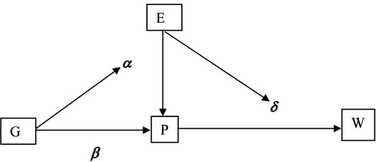
Suppose, say, a population of plants, each of which is either tall (P = t) or short (P = s). The phenotypic variable P is partly determined by a genetic variable G: some plants have a genotype that generates tall plants in any environment (G = t), others a genotype that generates short plants in any environment (G = s), and some a genotype (G = p) that generates tall plants in some environments and short plants in others. Let the relevant environmental condition E be the amount of light incident on the growing plant, so that in dim light (E = d) the plant grows tall, while in bright light (E = b) the plant remains short. It follows immediately that E is an interactive cause of P—the effect of E on P depends on the value of G for any particular plant (E has an effect if G = p but none at all if G = t or G = s).
We suppose that this plasticity comes at a direct cost to fitness; that is, the fitness of a phenotype is smaller if produced by a G = p genotype than by a G = s or G = t genotype (see n. 3 below). In consequence, E (or some correlate; see Huber et al. Reference Huber, Kane, Heschel, von Wettberg, Banta, Leuck and Schmitt2004) must be an interactive cause of absolute fitness W if a plastic phenotype is to evolve. For suppose E is not an interactive cause of fitness, and let Wg,e be the fitness of genotype g in environment e. We then have

(i.e., the difference in fitness induced by switching environments is identical for all genotypes, and in particular for the s and t genotypes). Without loss of generality, suppose tall plants are fitter than short plants in low-light environments, so that Ws,d < Wt,d. It then follows that tall plants are fitter than short plants in all environments. Further, given that plasticity comes at a cost, plants with G = p are less fit than plants with G = t, and a fixed rather than plastic phenotype goes to fixation.
The above constraints then impose a minimal causal structure required for the evolution of plasticity as an adaptive response to environmental variation, given in figure 1. Path coefficients represent the magnitude of the influence of a cause on its effect, and edges from a variable (e.g., G) to a coefficient on a path between two others (e.g., α on the path E → P) indicate an interactive dependence: the first variable (G) controls the degree (α) to which the second (E) influences the third (P).
Minimal causal structure required for adaptive evolution of plasticity.

Given this causal structure, what is required for G = p to evolve? Suppose (again without loss of generality) that tall plants are fitter than short plants in dim-light environments, but the reverse is true in bright-light environments. Because of the cost of plasticity, plants with G = p are less fit than plants with G = t in dim environments, but enjoy an advantage over them in bright environments, and similarly are less fit than plants with G = s in bright environments but more fit in dim environments. Thus, the advantage of the G = p type over the G = t type depends on the frequency of bright environments, and similarly the advantage of the G = p type over the G = s type depends on the frequency of dim environments. If plasticity is to evolve, plastic plants and competing fixed tall plants must end up in bright environments often enough to compensate for the disadvantage plastic plants have in dim environments, but at the same time plastic plants and competing fixed short plants must end up in dim environments often enough to compensate for the disadvantage of plastic plants in bright environments. That is to say, to determine whether plasticity will evolve as an adaptation, one must be in a position not only to specify the absolute fitnesses of each type in each environment but to specify as well the joint frequency distribution of types to environments. The question, then, is whether one can do this by appealing to environments as individuated not by the variable E itself—by whether light is bright or dim—but by a measure of quality, Q, specified for particular locations.
The answer is that one cannot in general do this. Absolute fitness depends interactively on E, and Q must track the absolute fitness of types at locations. But E need not and in general will not be identical for all individuals within a location; for example, the light levels for a given individual within a location may depend on the average height of its immediate neighbors. Given that E varies within a location, the distribution of E over types in the location will in general change as the frequency of types within the location changes, and so too will the resulting Q values. Thus, as plastic plants increase or decrease in frequency within a location, the Q values of the location will change as well. Predicting the fate of a plastic trait then depends on forecasting the distribution of Q values over physical locations, and the best way to do that is to measure the causes of Q and incorporate them into the model. Those causes include E or, in lieu of E, its causes, that is, yet other environmental features. In either case, there is no substitute for explicit representation of causally relevant environmental features.Footnote 3
Matters are not improved when we turn to explanation, that is, determining whether a plastic trait has evolved as an adaptation: G = p can be an adaptive response to variation in some E only if E is an interactive cause of both P and W. One cannot determine whether any particular E, or any E at all, plays either role without actually measuring it. And Q will not substitute here—it can play proxy for W (since it, by assumption, tracks absolute fitness) but not for E. One might think to avoid explicit measurements of E by simply tracking changes in absolute fitness: if the difference in fitness of tall plants between locations is not identical to the difference in fitness of short plants between locations (i.e., fitness is a nonseparable function of phenotype and location), this can be explained by appeal to an interactive causal dependence between an unmeasured environmental condition E and fitness. Unfortunately, such patterns in the variance of type fitness are also explicable by noninteractive dependencies between multiple unmeasured environmental variables E1, E2, and fitness, provided E1 and E2 covary with phenotype and location in the right way. To determine the presence of an interactive dependence, one must therefore either measure the interactive cause E or measure sets of possible noninteractive environmental causes to ensure that they do not account for the nonseparable fitness functions. Either way, there is no substitute for explicit representation.
Hence, to predict the evolutionary fate of plasticity, or to test its status as an adaptation, one must know the joint distribution over environment, genotype, and phenotype and the absolute fitnesses that obtain for each possible pairing of the three (Via and Lande Reference Via and Lande1985; van Tienderen Reference van Tienderen1991; Gomulkiewicz and Kirkpatrick Reference Gomulkiewicz and Kirkpatrick1992). This is possible only if relevant environmental features are explicitly represented and their causal influence modeled. While the importance of understanding interactive dependencies between environmental, genotypic, and phenotypic variables and fitness is particularly prominent when modeling the evolution of plasticity, the need to model these relations is actually quite general, and empirical examples are now available in the literature (e.g., Wilson et al. Reference Wilson, Pemberton, Pilkington, Coltman, Mifsud, Clutton-Brock and Kruuk2006).
6. Definitions
So far I have argued that, at least sometimes, we require explicit representation of environmental variables and their causal influence on fitness or its components. That raises a number of questions about the nature of these variables. The first is whether they should be measured on individual organisms or on populations of organisms. The answer is both.
It is commonly the case that within a population, environmental variables have different values for different individuals. So, for example, while the mean rainfall may be the same for all members of a local population of forbs occupying a given meadow, the seedling density, soil salinity, and even average soil moisture content may differ from spot to spot, and hence from plant to plant, in the local population. More generally, environmental features occurring at different scales causally influence survival and reproductive success, as well as community assembly, and in general, the smaller the scale of a feature, the fewer the number of individuals in a population that are influenced by any particular feature (see, e.g., Bossenbroek, Wagner, and Wiens Reference Bossenbroek, Wagner and Wiens2005). Consequently, in the first instance, environmental variables must be measured on individuals, even though they characterize features of the environment occupied by the individual. Once this is recognized, it is simple enough to note that the environment occupied by a given individual is characterized by a vector of values for some set of environmental variables and that any given vector may characterize many members of a population or only one member or none.
One is often interested, however, in some characterization of the environment occupied by the whole population. A suitable representation of such an environment can be constructed by considering the frequency distribution of environmental variables over members of the population. So, for example, the environment occupied by our population of forbs may be specified by the number of individuals characterized by each possible individual environment or more generally by the joint frequency distribution of the measured environmental variables. Frequencies are, of course, properties of populations, and so the variables here must be measured on populations.
Let us call a vector of values for environmental variables characterizing a given individual an individual environment. Similarly, let us call the joint frequency distribution of environmental variables over individuals in a population a population environment. Individual environments are useful for predicting the survival and reproductive success of individuals, conditional on the actual external circumstances they face. Population environments are constructed from a collection of individual environments and are useful for predicting demographic variables for the population, conditional on the actual circumstances faced by each member of the population.
If one wants to predict evolutionary outcomes, however, one needs more information: one needs not only to measure the current state of the environment but also to predict its future state. To do this, a probability distribution over the population's environment is required. Indeed, because in some species individuals migrate and their dispersal is often influenced by environmental variables, it is sometimes important to consider the probability distribution characterizing the chances that a given individual will come to occupy a particular individual environment. Following Glymour (Reference Glymour2006), let us denote by narrow environment, an environment specified by actual values for environmental variables, and by wide environment, an environment specified by a probability distribution over values for environmental variables.
We now have four distinct conceptions of an environment. Environmental variables are variables that causally influence survival, reproductive success, or community assembly, whose values characterize some feature of the world that pretheoretically counts as part of the environment or habitat occupied by one or more individual organisms. A narrow individual environment is a vector of values for environmental variables characterizing the habitat occupied by a particular individual organism. A wide individual environment is a probably density over all such vectors, where this density characterizes the chances that a particular individual will occupy a habitat characterized by particular values for the environmental variables. A narrow population environment is a joint frequency distribution over environmental variables, characterizing the frequency with which members of a given population occupy specific narrow individual environments. A wide population environment is a probability density over narrow population environments, where this density characterizes the chances that a given population will occupy specific narrow population environments over time.
7. Explicit Representation and Local Coadaptation
If the foregoing is correct, then biological modeling sometimes requires that we explicitly represent environments as vectors of values for variables that causally influence survival and reproductive success of individual organisms but also requires that we sometimes represent environments as frequency or probability distributions over those variables. It is worth illustrating the need for both kinds of representation. I will do so by considering the geographic mosaic theory of coevolution (GMTC; Thompson Reference Thompson1994).
The GMTC begins with the insight that species comprise genetically distinct subpopulations occupying different biotic environments, and within these subpopulations the interactions among species have different effects on survival and reproductive success. These local differences in the interactions between species will lead to coevolution between the species at some, but not all, locations. GMTC is proposed as an explanation for the distribution of the resulting local coadaptations. These patterns are best explained, according to the GMTC, by a three-part theory: “(1) There is a selection mosaic among populations, favoring different evolutionary trajectories to interactions in different populations. (2) There are coevolutionary hotspots, which are the subset of communities in which much of the coevolutionary change occurs. (3) There is a continual population remixing of the range of coevolving traits” (Thompson Reference Thompson1997, 1619).
If the GMTC is correct, one should expect that (a) the traits of interacting species will be coevolved to increase the fitness of both species in some local populations but not in others and that (b) most coevolved traits will not be ‘species level’; that is, most such traits will not be favored in all contexts but rather favored by just enough, in just enough subpopulations, to have evolved. Many of the predicted ecological patterns have been confirmed in various studies (Thompson Reference Thompson1997; Benkman, Holimon, and Smith Reference Benkman, Holimon and Smith2001; Brodie, Ridenhour, and Brodie Reference Brandon, Antonovics and Brandon2002).
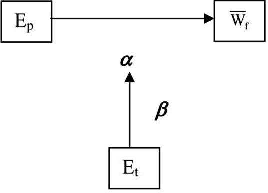
Unfortunately, the patterns can be generated by mechanisms other than the GMTC (Gomulkiewicz et al. Reference Gomulkiewicz, Drown, Dybdahl, Godsoe, Nuismer, Pepin, Ridenhour, Smith and Yoder2007). Hence, to test the GMTC, one must test the specific mechanisms it postulates. One of these is the context dependence of fitness functions for one focal species, where the interacting cause controlling the context is the trait frequency current in the local population of some interacting species. To illustrate, suppose a given trait variable P influences the fitness Wf in a given focal species F, in a frequency-dependent fashion. Let Ep be the frequency distribution of this trait in the local population of F. At the population level, Ep will be a cause of mean fitness for types,  , in local populations of F. Suppose further that there is an interacting species S with some polymorphic trait variable T, whose mean value in the local population of S we denote by Et. Finally, let Et be an interactive cause with Ep of
 , so that the causal structure is as in figure 2.
Interactive causal structure postulated by geographic mosaic theory of coevolution.

Then the extent to which P is adaptive for members of F depends on the local frequency of T in species S—it may be, for example, that in some locations this frequency is high, and the local population of F adapts by moving to a near optimal value for P; in other local populations, the local frequency of T is low, and in these populations P does not evolve but drifts in response to gene flow and selection on correlated traits. To test for the presence of this mechanism is to test for the presence of an interactive causal dependence between Et (the frequency distribution of T in the interacting species S) and  mediated by the functional dependence of
 on Ep.
To test the GMTC, then, one must identify the causal dependencies between fitness and specific environmental variables and, in particular, the presence or absence of interactive causation. To do this, one must explicitly represent the relevant environmental features, here, the trait frequencies in local subpopulations of species interacting with the focal species. However, locations will differ both over time and among themselves with respect to the trait distributions characterizing local populations of interacting species. Thus, it is not just that individuals do not occupy a common narrow individual environment, but further local populations of the focal species do not occupy the same narrow population environment. Because the frequencies of P and T in local populations of F and S change in response to one another over time, in order to predict the evolutionary fate of the species F, one needs a joint probability distribution over narrow population environments as individuated by these frequencies. That is, one requires wide population environments.
Before we return to the idea of adaptation to a particular environment, it is worth pausing to note one further implication of the mosaic theory of local coevolution. Wide population environments are always definable for a species, no matter how heterogeneous the individual environments occupied by its members may be. Any two members of the same species, then, can be said to share an environment in the trivial sense that they are both members of the same species, characterized by just one wide population environment. It is sometimes said that selection presupposes a common environment; to the extent that the environment in question is a wide population environment, this is true. But, as we saw above, narrow environments need not be shared: selection can act on a collection of individual organisms that share neither narrow individual nor narrow population environments. To insist otherwise is to rule out a priori the possibility of local coadaptation. While it may be true that a common environment is a necessary condition for selection, this is true only for environments conceived in particular ways and need not hold on other, equally cogent, conceptions.
8. Environment and Adaptation
As we have seen, interactive causes play a crucial role in the evolution of plasticity and local coadaptations. This is no accident—both involve adaptation to environmental conditions, and interactive causes play an essential role in such adaptation. I now turn to the argument for this claim.
Species (or populations) adapt to environmental conditions, while individual organism bear adaptations. On one view of things, species adapt to the totality of environmental circumstances faced by members of the species (i.e., to population environments). This view is deeply holistic, in that it recognizes that the adaptive phenotypes of individual organisms are constrained not by one or a few features of the environment but by the whole of it: to the extent that a given environmental feature drives change in a particular phenotypic trait, changes in that trait are themselves constrained by yet other environmental features driving change (or stasis) in yet other phenotypic traits sharing common genetic or developmental pathways with the first. On this view of adaptation, it is importantly misleading to see any given phenotype simply as an adaptation to any particular environmental condition.
The ideas of selective environments and selective neighborhoods comport well with this conception of adaptation and adaptations. Using measures of environmental quality, one can identify the phenotypic traits whose evolution is governed in part or in whole by selective processes and that, hence, count as adaptations. As we will see below, it will not be possible to identify particular features of the environment as important causes of differential fitness, and so to identify particular phenotypic traits as adaptations to those features, but the associated conception of adaptation does not demand, in fact discourages, any such identification.
On another view of things, it is just this idea that adaptations are sometimes adaptations to particular environmental conditions that is crucial. This conception of adaptation locates particular features of the environment as responsible for, and hence explanatory of, particular adaptive changes. So, for example, hypsodonty (high-crowned teeth) in ungulates has been explained as an adaptation to abrasive material in the food supply characteristic of grassland environments (McFadden Reference McFadden1992; Heywood Reference Heywood2010), while bipedalism in hominids has been explained alternatively as a thermoregulatory adaptation to an open savanna equatorial environment (Wheeler Reference Wheeler1991) and as a feeding adaptation to a woodland environment (Hunt Reference Hunt1994). Once identified, the environmental conditions and their associated adaptations can sometimes be used to predict and explain macroevolutionary patterns (see, e.g., Heywood Reference Heywood2010). Thus, the idea of adaptation to particular conditions is deeply ingrained in biological practice.
Unlike the first, holistic, conception of adaptation, this second view of adaptation is reductionist, identifying some but not all environmental conditions as especially relevant to the evolution of particular phenotypes. While apparently at odds, the two conceptions of adaptation are not necessarily incompatible. If the first recognizes the existence of multiple interacting environmental, genetic, and developmental constraints on the evolution of any given phenotype, the second gives us a way of representing those constraints. The reconciliation trades on the essential role of interactive causes in the process of adaptation, the identification of which in turn requires the more fine-grained conceptions of environment emerging from the strategy of explicit representation.
The necessity of interactive causes can be put simply. If we are to identify one rather than another feature of the environment as the feature to which a species is adapting, that feature must explain differences in fitness among phenotypes, even when it is homogeneously distributed over types in the population. This is only possible if the environmental feature is an interactive cause of fitness or its components. But if the saying is easy, the seeing may be harder. A series of examples will help.
Suppose we have a population of two perfectly heritable phenotypes, P = 1 and P = 2—say 12 of each—distributed over narrow individual environments defined by two environmental variables, each with two states: E1 = 1 or 2, E2 = 1 or 2. Suppose the distribution is homogenous for each type (i.e., the populations composed of the distinct types share a narrow population environment), with say three of each type in each narrow individual environment (which are, for the sake of clarity, <E1 = 1, E2 = 1>, <E1 = 1, E2 = 2>, <E1 = 2, E2 = 1>, and <E1 = 2, E2 = 2>). Finally, suppose the number of offspring produced by an individual is given by the linear additive function W = 3 + 2P + E1 − E2 and that offspring are chosen at random to repopulate the habitat after each episode of reproduction. Both E1 and E2 causally influence fitness, but neither does so interactively (the contributions of E and P are separable). Barring drift, this population will quickly go to fixation for P = 2 individuals (the average absolute fitness of P = 1 being 5, while that of P = 2 is 7). But there is no clear sense in which P = 2 is an adaptation to E1 as opposed to E2 or conversely. By changing the value of either, we can change the relative fitness of P = 1; for example, we can by increasing the value of E1 over the population, say by one unit, increase the relative fitness of P = 1, thereby decreasing the selection differential and slowing the speed of evolutionary change. But (modulo a change in sign) the same is true for E2—uniformly increasing E2 increases the selection differential. Importantly, we cannot by any uniform modification of either environmental variable change the fact that P = 1 is less fit than P = 2.
So environmental conditions like E1 and E2 can change the speed with which an evolutionary outcome is reached, but they can change that outcome only if they are nonhomogeneously distributed over types. So, for example, we could ensure (again barring drift) that the population remains polymorphic by fixing things so that the P = 1 phenotype invariably found its way into E1 = 2, E2 = 1 environments, while the P = 2 phenotype invariably found itself confronted by the less fortuitous E1 = 1, E2 = 2 environment (both types then having an absolute fitness of 6). But, as Brandon (Reference Boughton1990) has argued, if this differential distribution of environments occurs by accident, any resulting evolutionary state is a consequence of drift, not adaptation. And if the differential distribution of environments occurs as a result of habitat preferences, it is not values of P that are adaptations but rather the habitat preferences that lead P = 1 phenotypes to particularly favorable physical environments.
The upshot is that unless one can explain differences in the absolute fitness of alternative phenotypes by appeal to a shared environmental condition, there is no sense in which a phenotype can be an adaptation to that condition in particular. Clearly, environments individuated by measures of quality assessment, and selective environments in particular, can perform no such explanatory chore, being defined by the very differences in need of explanation. Happily, such explanations are possible—explanations of different outcomes by appeal to shared conditions—but only if the shared conditions are interactive causes of the outcomes.
To see how this works, suppose the fitness function in our above example is W = 3 + 2P + E1 − PE2; here, P and E2 are interactive causes of fitness in virtue of the last term on the right-hand side. When narrow individual environments are homogeneously distributed as above, the resulting type fitnesses are 5 and 5.5 for the P = 1 and P = 2 phenotypes, respectively, and again the population goes to fixation for P = 2. And as before, while uniform interventions on E1 can change the speed with which the population evolves, they cannot forestall the eventual fixation of P = 2. For example, uniformly increasing E1 by one unit yields absolute fitnesses of 6 and 6.5 for P = 1 and P = 2, with a resulting selection differential of .077 rather than .09.
But now consider an intervention that uniformly increases E2 by one unit. The absolute fitness of the P = 1 phenotype becomes 4, while that of P = 2 becomes 3.5: relative fitnesses are reversed, and barring drift, P = 1 evolves. A change in E1 cannot influence the ordinal relation between absolute fitnesses of the types, and so its value cannot explain differences in type fitness—in any given context, the ordinal relation of type fitnesses would have remained the same, no matter what the (homogenous) distribution of E1 values might be. But because E2 is an interactive cause, a change in its value can influence the ordinal relations between fitnesses, and hence its value can explain differences in type fitnesses. The evolution of P = 1 rather than P = 2 in the original (E2 values of 1 and 2) narrow population environment is explained (in part) by the homogeneous distribution of E2 values because, had they been different—as in the novel narrow population environment (E2 values of 2 and 3)—the ordinal relations among type fitnesses, and hence the evolutionary outcome, would have been different. Here it seems right to say that once a population has reached fixation for P, the fixed value of P, whichever it may be, is an evolved response to the particular distribution over E2 confronted by the population.
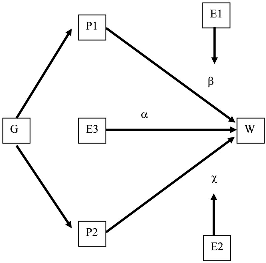
We have, then, a vindication of the reductive idea that adaptations are sometimes adaptations to particular environments. Can the vindication lead us to an integration of the reductive and holistic conceptions of adaptation? Consider the causal graph in figure 3. We have two phenotypic variables, P1 and P2, with a common genetic or developmental cause G. Both causally influence fitness. We also have three environmental variables, E1, E2, and E3. All three causally influence fitness: E1 and E2, by controlling the magnitude of the influence of P1 and P2, respectively, and E3, directly and noninteractively.
Environmental constraints on adaptation.

From the above discussion, we can identify E3 as an environmental condition that is relevant to evolutionary dynamics—it influences the rate of evolution—but that cannot explain one evolutionary outcome as against another unless it happens to have a nonhomogeneous distribution over types. Condition E3 causes fitness, but it is not an environmental feature to which a population can adapt. Conversely, E1 and E2, being interactive causes of fitness, represent environmental conditions to which populations can adapt. In particular, an evolved value for P1 is an adaptation to the value of or distribution over E1, while the evolved value for P2 is an adaptation to the value of or distribution over E2. But what shall we say of the relation between E2 and P1?
Clearly, E2 is relevant to the evolution of P1 but differently so than either E1 or E3. Unlike E3, E2 can influence not only the rate of evolution but also the evolutionary outcome with respect to P1. But this influence is structurally different from that of E1. The effect of P1 on W depends on E1 but not on E2; hence, changes in the value of E1 can change the optimal value of P1, but changes in the value of E2 have no such consequence. However, to the extent that P1 and P2 share a common genetic cause G, the optimal value of P1 and the optimal value of P2 may not be co-obtainable. In this case, selection drives G to the optimal trade-off between P1 and P2 values, and the strength of this selection on G is a function of the influence of both P1 and P2 on fitness. The latter influence is controlled by E2, and in this way, E2 can, unlike E3, constrain the evolution of P1. If we then take E2 to be an environmental constraint on the evolution of P1, we have a principled distinction between the roles of E1, E2, and E3 in the evolution of P1.Footnote 4
The foregoing distinction between an environmental feature to which a species adapts and features constraining that adaptive response rests on a discoverable difference in the structure and functional form of causal dependencies. To the extent that such constraints are ubiquitous, the holistic insight will be vindicated, at least in part: species adapt to the totality of the environmental contingencies their members face, and no particular phenotype can be understood as an optimized response to any particular environmental exigency. But this insight is nonetheless compatible with the idea that some environmental conditions are more nearly relevant for understanding the evolution of particular phenotypes—these are the conditions to which the phenotypes are adaptations because these environmental conditions directly control the influence of the phenotypes on fitness and thereby influence the optimal value of the relevant trait variables. Environmental constraints, conversely, influence the phenotype that is fixed not by directly influencing which value of the trait variable is, ceteris paribus, optimal but by imposing indirect costs on organisms that in fact realize the otherwise optimal value for the trait variable.
9. Concluding Remarks and a Final Caveat
The forgoing arguments show that in some contexts the presence of interactive environmental causes forces the use of explicit representation in preference to quality assessment when modeling environments, as, for example, determining whether a plastic phenotype is an adaptation and testing the mosaic theory of local coevolution. The move to explicit representations incurs some epistemic costs, if only because the resulting models are more complex and therefore require the use of more detailed data than would otherwise be necessary. However, the added complexity permits the identification of particular environmental conditions to which phenotypes are adaptations, thus saving a principled notion of ‘adaptation to’.
Three caveats are in order. First, while many interactive environmental causes of fitness will vary over the geographic distribution of a species, some will be relatively stable over the life of a species. Others will be relatively stable over even longer stretches of geological time, and perhaps some may even be stable over the entire history of life. The stability of such variables does not preclude talk of adaptation to the environmental conditions represented by their values, nor does it vitiate the explanatory power of the designation ‘adaptation to’. That such an environmental variable has the value it does may serve to explain why one phenotype is fitter than alternatives, even when the variable is constant in value.Footnote 5
Second, as was noted above, if it is organisms that bear adaptations, it is species that do the adapting. To the extent that a fixed phenotype, stable polymorphism, or speciation event is a consequence of the adaptive process, there is a clear sense in which such species-level properties are adaptations—they are characters possessed by the species as an adaptive response to the environmental exigencies faced by the species. Perhaps not all are willing to go so far as to recognize such characters as species-level adaptations. But some will be, and for them it is important to note that nothing I have said here shows that interactive dependencies between environmental conditions and fitness are necessary conditions of species-level adaptations, so understood. That they are seems a reasonable conjecture, but consideration of it is beyond the scope of this article.
Third, my arguments urge that potential environmental causes of fitness be explicitly measured but offer little guidance in the choice of specific variables to measure. Principles offering reliable a priori advice about variable selection would be wonderful, at once solving Goodman's new riddle while offering useful advice to working scientists. Alas, such principles are few and far between, and I, at least, have none to offer. The choice to measure one rather than another set of variables must be guided by expert judgment, empirically corrected by pilot studies of one kind or another, for example, phytometer studies as described by Brandon and Antonovics (Reference Brandon1996), or other observational and experimental work on the population of interest.