





1. Introduction
The flow of electrically conducting fluids is of interest in many applications. Examples range across length scales, from microfluidics to the flow of liquid metals in casting. Notably, liquid metals are a strong candidate for coolant applications in fusion technology (Hong-yan, Yi-can & Xiao-xong Reference Hong-yan, Yi-can and Xiao-xong2002; Smolentsev, Moreau & Abdou Reference Smolentsev, Moreau and Abdou2008). In many of these cases, the flow is subject to strong applied magnetic fields and the coupling between the flow field and the magnetic field can have significant affects on the flow itself, with concomitant affects on flow profiles, pressure drop and heat transfer (Davidson Reference Davidson2001; Müller & Bühler Reference Müller and Bühler2001). The ability to predict such effects is essential to the development of devices which make use of these phenomena. For both heat and mass transfer applications, conducting fluids may be driven through arrangements of ducts and it is important to fully understand the properties of such flows, as they differ markedly from their non-magnetohydrodynamic (MHD) counterparts. However, MHD presents challenges in all of these areas, over and above that of conventional fluid dynamics: experimental studies (e.g. Xu et al. Reference Xu, Pan, Zhang, Zhao, Zhang and Yang2009; Smolentsev et al. Reference Smolentsev, Xu, Pan and Abdou2010) are difficult due to the opaque nature of most conducting fluids and molten metals, and the environment is extremely harsh, which presents issues in regard to instrumentation. Computational MHD (CMHD) (Smolentsev, Morley & Abdou Reference Smolentsev, Morley and Abdou2005) must include additional equations for the electromagnetic field; the fields outside of the fluid region (fringing fields) have significant affects and must be modelled appropriately; strong magnetic fields can cause turbulence suppression, a breakdown in assumptions of isotropy, the generation of wall and free shear layers and the boundary layer behaviour can be particularly difficult to resolve at Hartmann walls. Due to the challenges inherent in CMHD and the relative paucity of experimental results, there is considerable need for analytical solutions, not least for the purposes of validation (Tao & Ni Reference Tao and Ni2013b ).
For fully developed flow in a single rectangular duct, a number of analytical solutions exist, developed by Shercliff (Reference Shercliff1953) and Hunt (Reference Hunt1965). These assume axial, laminar flow and neglect the effects of finite length, thermal convection and instabilities of the side-wall jets. A number of variations on these treatments have followed (Hunt & Stewartson Reference Hunt and Stewartson1965; Hunt & Leibovich Reference Hunt and Leibovich1967; Temperley & Todd Reference Temperley and Todd1971; Müller & Bühler Reference Müller and Bühler2001). In all of these cases it is assumed that the wall is thin in comparison with the duct width. Recent work in this area has extended these ideas to thick-walled ducts (Tao & Ni Reference Tao and Ni2013a ,Reference Tao and Ni b ).
A related problem arises in fusion blanket design where the coolant pathway consists of arrays of parallel ducts (e.g. Madarame, Taghavi & Tillack Reference Madarame, Taghavi and Tillack1985). Conducting walls can lead to electromagnetic coupling between ducts, influencing the hydrodynamic behaviour. Variations on this problem have been analysed numerically (McCarthy & Abdou Reference McCarthy and Abdou1991; Gaizer & Abdou Reference Gaizer and Abdou1996; Zhang, Pan & Xu Reference Zhang, Pan and Xu2014) and by singular perturbation theory (Molokov Reference Molokov1993). McCarthy and Abdou developed an iterative numerical method for ducts with conducting walls (side and Hartmann) stacked parallel to the applied magnetic field, as is the case here. Molokov developed an asymptotic solution valid for large
 $\mathit{Ha}$
for the case with ducts stacked perpendicular to the applied magnetic field. The most recent work by Zhang et al. employed a numerical solution to study both arrangements for two ducts and the parallel arrangement for three ducts. To the best of the authors’ knowledge, analytical solutions valid for arbitrary
 $\mathit{Ha}$
, as proposed here, do not exist for these problems.
This work presents an analytical solution to a generalized Hunt-type problem with ducts stacked parallel to the applied magnetic field, where the ducts have non-conducting side walls and arbitrary thickness conducting Hartmann walls. Such analytical solutions aid in our understanding of these flows and provide important benchmarking and validation data for computational MHD, as well as providing approximate flow parameters for 1D systems codes. In § 2 the quasi-static, laminar, fully developed flow equations are derived for the case of a thick-walled duct. An analytical result is obtained for the relevant hydrodynamic and magnetic parameters for the single duct with thick walls using a separation of variables method in § 3, and the limitations of the thin-wall approximation (developed by Hunt) are demonstrated. These results are then extended to an array of ducts stacked in the direction of the applied magnetic field in § 4. An investigation of these solutions for two, three and five parallel ducts in both co- and counter-flow configurations is given in § 5. The coupling between ducts and its impact on the hydrodynamics is studied in detail, in both co- and counter-flow configurations. It is seen that the conducting walls have a strong influence on the Lorentz forces near the wall, giving rise to significant enhancement of wall shear stresses in the co-flow case and strong suppression in the counter-flow case. In certain circumstances, flow reversal of the core flow (relative to the pressure gradient) can be obtained, resulting in counter-current flow.
2. Formulation
We begin by considering the flow of an incompressible electrically conducting fluid of kinematic viscosity
 ${\it\nu}$
, density
 ${\it\rho}$
, electrical conductivity
 ${\it\sigma}_{f}$
and permeability
 ${\it\mu}_{f}$
. The fluid velocity
 $\boldsymbol{u}$
satisfies the following momentum equation:
 $$\begin{eqnarray}\frac{\partial \boldsymbol{u}}{\partial t}+\boldsymbol{u}\boldsymbol{\cdot }\boldsymbol{{\rm\nabla}}\boldsymbol{u}=-\frac{1}{{\it\rho}}\boldsymbol{{\rm\nabla}}p+\frac{{\it\nu}}{{\it\rho}}{\rm\nabla}^{2}\boldsymbol{u}+\frac{1}{{\it\rho}}\boldsymbol{j}\times \boldsymbol{B}\end{eqnarray}$$
together with
 $$\begin{eqnarray}\boldsymbol{{\rm\nabla}}\boldsymbol{\cdot }\boldsymbol{u}=0\end{eqnarray}$$
where
 $p$
is the pressure,
 $\boldsymbol{j}$
is the current density and
 $\boldsymbol{B}$
is the magnetic induction (although the term magnetic field is used where no confusion with
 $\boldsymbol{H}$
can arise). The magnetic (and electric) fields (
 $\boldsymbol{H}$
and
 $\boldsymbol{E}$
respectively) are governed by the Maxwell equations (Davidson Reference Davidson2001). Ignoring the displacement current, Maxwell’s equations together with Ohm’s law state that
 $$\begin{eqnarray}\boldsymbol{{\rm\nabla}}\times \boldsymbol{H}=\boldsymbol{j}={\it\sigma}_{f}(\boldsymbol{E}+\boldsymbol{u}\times \boldsymbol{B})\end{eqnarray}$$
where
 $$\begin{eqnarray}\boldsymbol{B}={\it\mu}_{f}\boldsymbol{H}.\end{eqnarray}$$
Taking the curl of (2.3) and using the constitutive law (2.4), together with the fact that
 $\boldsymbol{{\rm\nabla}}\boldsymbol{\cdot }\boldsymbol{B}=0$
gives
 $$\begin{eqnarray}-\!\frac{1}{{\it\mu}_{f}{\it\sigma}_{f}}{\rm\nabla}^{2}\boldsymbol{B}=\boldsymbol{{\rm\nabla}}\times \boldsymbol{E}+\boldsymbol{{\rm\nabla}}\times (\boldsymbol{u}\times \boldsymbol{B}).\end{eqnarray}$$
Since
 $$\begin{eqnarray}\boldsymbol{{\rm\nabla}}\times (\boldsymbol{u}\times \boldsymbol{B})=\boldsymbol{u}(\boldsymbol{{\rm\nabla}}\boldsymbol{\cdot }\boldsymbol{B})-\boldsymbol{B}(\boldsymbol{{\rm\nabla}}\boldsymbol{\cdot }\boldsymbol{u})+(\boldsymbol{B}\boldsymbol{\cdot }\boldsymbol{{\rm\nabla}})\boldsymbol{u}-(\boldsymbol{u}\boldsymbol{\cdot }\boldsymbol{{\rm\nabla}})\boldsymbol{B}\end{eqnarray}$$
and
 $$\begin{eqnarray}\boldsymbol{{\rm\nabla}}\boldsymbol{\cdot }\boldsymbol{B}=\boldsymbol{{\rm\nabla}}\boldsymbol{\cdot }\boldsymbol{u}=0\end{eqnarray}$$
it follows that
 $$\begin{eqnarray}\boldsymbol{{\rm\nabla}}\times (\boldsymbol{u}\times \boldsymbol{B})=(\boldsymbol{B}\boldsymbol{\cdot }\boldsymbol{{\rm\nabla}})\boldsymbol{u}-(\boldsymbol{u}\boldsymbol{\cdot }\boldsymbol{{\rm\nabla}})\boldsymbol{B}.\end{eqnarray}$$
The other Maxwell equation is given by
 $$\begin{eqnarray}\boldsymbol{{\rm\nabla}}\times \boldsymbol{E}=-\frac{\partial \boldsymbol{B}}{\partial t}.\end{eqnarray}$$
Substituting (2.9) and (2.8) into (2.5) gives the well-known induction equation (Davidson Reference Davidson2001) for
 $\boldsymbol{B}$
,
 $$\begin{eqnarray}\frac{\partial \boldsymbol{B}}{\partial t}=\frac{1}{{\it\mu}_{f}{\it\sigma}_{f}}{\rm\nabla}^{2}\boldsymbol{B}+(\boldsymbol{B}\boldsymbol{\cdot }\boldsymbol{{\rm\nabla}})\boldsymbol{u}-(\boldsymbol{u}\boldsymbol{\cdot }\boldsymbol{{\rm\nabla}})\boldsymbol{B}.\end{eqnarray}$$
Decomposing the magnetic field into a spatially uniform, time independent applied component
 $\boldsymbol{B}^{0}$
, and an induced component
 $\boldsymbol{B}^{i}$
such that
 $\boldsymbol{B}=\boldsymbol{B}^{0}+\boldsymbol{B}^{i}$
, then
 $$\begin{eqnarray}\frac{\partial \boldsymbol{B}}{\partial t}=\frac{\partial \boldsymbol{B}^{i}}{\partial t},\quad {\rm\nabla}^{2}\boldsymbol{B}={\rm\nabla}^{2}\boldsymbol{B}^{i}.\end{eqnarray}$$
If it is now assumed that the magnetic Reynolds number
 $Re_{m}={\it\mu}_{f}{\it\sigma}_{f}LU$
is small, where
 $L$
and
 $U$
are the characteristic length and velocity, then the induced field is small compared with the applied field, that is
 $\boldsymbol{B}^{0}+\boldsymbol{B}^{i}\approx \boldsymbol{B}^{0}$
, so one can write the second term on the right-hand side of (2.10) as
 $$\begin{eqnarray}(\boldsymbol{B}\boldsymbol{\cdot }\boldsymbol{{\rm\nabla}})\boldsymbol{u}-(\boldsymbol{u}\boldsymbol{\cdot }\boldsymbol{{\rm\nabla}})\boldsymbol{B}=(\boldsymbol{B}^{0}\boldsymbol{\cdot }\boldsymbol{{\rm\nabla}})\boldsymbol{u}-(\boldsymbol{u}\boldsymbol{\cdot }\boldsymbol{{\rm\nabla}})\boldsymbol{B}^{i}.\end{eqnarray}$$
The following expression for the induction equation is then obtained:
 $$\begin{eqnarray}\frac{\partial \boldsymbol{B}^{i}}{\partial t}+(\boldsymbol{u}\boldsymbol{\cdot }\boldsymbol{{\rm\nabla}})\boldsymbol{B}^{i}=\frac{1}{{\it\mu}_{f}{\it\sigma}_{f}}{\rm\nabla}^{2}\boldsymbol{B}^{i}+(\boldsymbol{B}^{0}\boldsymbol{\cdot }\boldsymbol{{\rm\nabla}})\boldsymbol{u}.\end{eqnarray}$$
If, in addition, it is assumed that a laminar, quasi-steady state case holds (i.e. an infinite interaction parameter), then the time derivatives and advection terms on the left-hand side of both the momentum equation (2.1) and induction equation (2.13) vanish. Further limiting our study to fully developed, axially directed, two-dimensional flows in square ducts, as shown in figure 1, we define
 $\boldsymbol{u}=(0,0,v)$
,
 $\boldsymbol{B}^{i}=(0,0,B_{z})$
and
 $\boldsymbol{B}^{0}=(B_{x}^{0},0,0)$
. The momentum equation in this square duct of side
 $2a$
with Hartmann wall thickness
 $w$
, insulated side walls, subject to an applied
 $X$
-directed magnetic field
 $B_{x}^{0}$
and driven by a pressure gradient
 $\partial p/\partial Z$
is then given by
 $$\begin{eqnarray}{\it\nu}\left(\frac{\partial ^{2}v}{\partial X^{2}}+\frac{\partial ^{2}v}{\partial Y^{2}}\right)-\frac{1}{{\it\rho}}\frac{\partial p}{\partial Z}+\frac{1}{{\it\rho}}\frac{1}{{\it\mu}_{f}}\frac{\partial B_{z}}{\partial X}B_{x}^{0}=0.\end{eqnarray}$$
Note that the last term on the left-hand side of this equation is the Lorentz force. The flow of conducting fluid generates an induced magnetic field
 $B_{z}$
, satisfying the following form of the induction equation, obtained from (2.13):
 $$\begin{eqnarray}\frac{1}{{\it\mu}_{f}{\it\sigma}_{f}}\left(\frac{\partial ^{2}B_{z}}{\partial X^{2}}+\frac{\partial ^{2}B_{z}}{\partial Y^{2}}\right)+B_{x}^{0}\frac{\partial v}{\partial X}=0.\end{eqnarray}$$
The magnetic field
 $B_{w}$
, in each wall satisfies
 $$\begin{eqnarray}\frac{\partial ^{2}B_{w}}{\partial X_{w}^{2}}+\frac{\partial ^{2}B_{w}}{\partial Y_{w}^{2}}=0\end{eqnarray}$$
where
 $(X_{w},Y_{w})$
denotes the coordinate system in each wall, as shown in figure 1. Non-dimensionalizing, by setting
Single thick-walled duct geometry.

 $$\begin{eqnarray}x=\frac{X}{a},\quad y=\frac{Y}{a},\quad z=\frac{Z}{a},\quad {\it\delta}=\frac{w}{a},\quad x_{w}=\frac{X_{w}}{a},\quad y_{w}=\frac{Y_{w}}{a},\end{eqnarray}$$
 $$\begin{eqnarray}\displaystyle & U=\displaystyle \frac{{\it\rho}{\it\nu}}{\left(\partial p/\partial Z\right)a^{2}}v & \displaystyle\end{eqnarray}$$
 $$\begin{eqnarray}\displaystyle & \mathit{Ha}=B_{x}^{0}a\sqrt{{\displaystyle \frac{{\it\sigma}_{f}}{{\it\rho}{\it\nu}}}} & \displaystyle\end{eqnarray}$$
 $$\begin{eqnarray}B=\frac{1}{{\it\mu}_{f}}\frac{1}{\left(\partial p/\partial Z\right)a^{2}}\sqrt{\frac{{\it\rho}{\it\nu}}{{\it\sigma}_{f}}}B_{z}\end{eqnarray}$$
it follows that
 $$\begin{eqnarray}\left(\frac{\partial ^{2}U}{\partial x^{2}}+\frac{\partial ^{2}U}{\partial y^{2}}\right)-1+\mathit{Ha}\frac{\partial B}{\partial x}=0\end{eqnarray}$$
with no-slip boundary conditions at the fluid–wall interface:
 $$\begin{eqnarray}U=0.\end{eqnarray}$$
Note that the final term on the left-hand side of (2.21) is a non-dimensional Lorentz force. This quantity will have an important role in the explanation of the mechanisms involved in this problem. The fluid magnetic field
 $B$
satisfies
 $$\begin{eqnarray}\left(\frac{\partial ^{2}B}{\partial x^{2}}+\frac{\partial ^{2}B}{\partial y^{2}}\right)+\mathit{Ha}\frac{\partial U}{\partial x}=0\end{eqnarray}$$
in the fluid region. Note that the Shercliff solution
 $U=U_{sh},B=B_{sh}$
, given in appendix A, satisfies these equations with homogeneous Dirichlet boundary conditions on
 $U$
and
 $B$
. One can then write
 $U=u+U_{sh}$
and
 $B=b+B_{sh}$
, and it follows that
 $$\begin{eqnarray}\left(\frac{\partial ^{2}u}{\partial x^{2}}+\frac{\partial ^{2}u}{\partial y^{2}}\right)+\mathit{Ha}\frac{\partial b}{\partial x}=0\end{eqnarray}$$
with no-slip boundary conditions at the fluid–wall interface:
 $$\begin{eqnarray}u=0\end{eqnarray}$$
whilst
 $b$
satisfies
 $$\begin{eqnarray}\left(\frac{\partial ^{2}b}{\partial x^{2}}+\frac{\partial ^{2}b}{\partial y^{2}}\right)+\mathit{Ha}\frac{\partial u}{\partial x}=0\end{eqnarray}$$
subject to appropriate homogeneous Dirichlet conditions on the side walls (
 $y=\pm 1$
) and interface conditions on the Hartmann walls (
 $x=\pm 1$
). The reason for using the decomposition of
 $U$
and
 $B$
above is to reduce the problem to a homogeneous case where the separation of variables method may be more easily applied.
The non-dimensional magnetic field in each wall,
 $b_{w}$
, satisfies
 $$\begin{eqnarray}\frac{\partial ^{2}b_{w}}{\partial x_{w}^{2}}+\frac{\partial ^{2}b_{w}}{\partial y_{w}^{2}}=0\end{eqnarray}$$
subject to boundary and interface conditions described in § 2.1.
It is convenient to express the velocity and fluid magnetic fields in terms of auxiliary variables
 ${\it\phi}$
and
 ${\it\psi}$
(known as the Elsasser variables), which has the attractive property of decoupling the equations:
 $$\begin{eqnarray}{\it\phi}=u+b,\quad {\it\psi}=u-b\end{eqnarray}$$
and by adding (and subtracting) the fluid equations it is seen that
 ${\it\phi}$
and
 ${\it\psi}$
satisfy:
 $$\begin{eqnarray}\displaystyle & \displaystyle \frac{\partial ^{2}{\it\phi}}{\partial x^{2}}+\frac{\partial ^{2}{\it\phi}}{\partial y^{2}}+\mathit{Ha}\frac{\partial {\it\phi}}{\partial x}=0 & \displaystyle\end{eqnarray}$$
 $$\begin{eqnarray}\displaystyle & \displaystyle \frac{\partial ^{2}{\it\psi}}{\partial x^{2}}+\frac{\partial ^{2}{\it\psi}}{\partial y^{2}}-\mathit{Ha}\frac{\partial {\it\psi}}{\partial x}=0. & \displaystyle\end{eqnarray}$$
2.1. Electromagnetic boundary and interface conditions
In the previous section, the problem is reduced to one involving the Elsasser variables,
 ${\it\phi}$
and
 ${\it\psi}$
. In principle, boundary and interface conditions are required in terms of these variables. In our approach, however, general solutions in terms of the Elsasser variables are obtained (subject only to homogeneity on the side walls) which are then subsequently reconstituted as
 $b$
and
 $u$
. The necessity for this is clear from the fact that the interface conditions will involve the wall magnetic field
 $b_{w}$
. As a result boundary and interface conditions are applied to the original variables. In the following we explain in detail how we arrive at these conditions.
The side walls (
 $y=\pm 1$
) are insulated and as a result the boundary condition on these walls is simply
 $$\begin{eqnarray}B=b+B_{sh}=0\Rightarrow b=0.\end{eqnarray}$$
Equations (2.24), (2.26) and (2.27) are coupled at the fluid-conducting wall interface
 ${\rm\Gamma}$
where continuity of field and flux are enforced. Hence,
 $$\begin{eqnarray}\displaystyle & \boldsymbol{n}\boldsymbol{\cdot }\boldsymbol{j}=\boldsymbol{n}\boldsymbol{\cdot }\boldsymbol{j}_{w} & \displaystyle\end{eqnarray}$$
 $$\begin{eqnarray}\displaystyle & \boldsymbol{n}\times (\boldsymbol{E}-\boldsymbol{E}_{w})=0 & \displaystyle\end{eqnarray}$$
 $$\begin{eqnarray}\displaystyle & \boldsymbol{n}\times (\boldsymbol{H}-\boldsymbol{H}_{w})=\boldsymbol{J}_{s} & \displaystyle\end{eqnarray}$$
 $\boldsymbol{j}_{w}$
,
 $\boldsymbol{E}_{w}$
and
 $\boldsymbol{H}_{w}$
are the current density, electric field and magnetic field in the wall, respectively. The surface current at the interface between the fluid and wall is denoted by
 $\boldsymbol{J}_{s}$
. For the case of a conductor/conductor interface, it must hold that
 $\boldsymbol{J}_{s}=\mathbf{0}$
. Substituting Maxwell’s equations into these give the following interface conditions which must apply at each interface:
 $$\begin{eqnarray}\boldsymbol{n}\boldsymbol{\cdot }\boldsymbol{{\rm\nabla}}\times \boldsymbol{H}=\boldsymbol{n}\boldsymbol{\cdot }{\boldsymbol{{\rm\nabla}}_{w}\times \boldsymbol{H}}_{w}\end{eqnarray}$$
and
 $$\begin{eqnarray}\frac{1}{{\it\sigma}_{f}}\boldsymbol{n}\times \boldsymbol{{\rm\nabla}}\times \boldsymbol{H}=\frac{1}{{\it\sigma}_{w}}\boldsymbol{n}\times {\boldsymbol{{\rm\nabla}}_{w}\times \boldsymbol{H}}_{w}\end{eqnarray}$$
on
 ${\rm\Gamma}$
, where
 $\boldsymbol{n}$
is a unit normal to the interface,
 ${\it\sigma}_{w}$
is the wall electrical conductivity and
 $\boldsymbol{{\rm\nabla}}_{w}$
indicates a gradient evaluated within the wall. It is convenient to define the wall conductance ratio
 $c_{w}$
as
 $$\begin{eqnarray}c_{w}=\frac{{\it\sigma}_{w}w}{{\it\sigma}_{f}a}=\frac{{\it\sigma}_{w}}{{\it\sigma}_{f}}{\it\delta}.\end{eqnarray}$$
In the case of interest, one can assume that
 $\boldsymbol{H}=\left(0,0,B/{\it\mu}\right)$
so
 $$\begin{eqnarray}\boldsymbol{{\rm\nabla}}\times \boldsymbol{H}=\frac{1}{{\it\mu}}\left(\boldsymbol{i}\frac{\partial B}{\partial y}-\boldsymbol{j}\frac{\partial B}{\partial x}\right).\end{eqnarray}$$
On Hartmann walls (
 $x=\pm 1$
), conditions (2.35) and (2.36) reduce to
 $$\begin{eqnarray}\frac{1}{{\it\mu}_{f}}\frac{\partial B}{\partial y}=\frac{1}{{\it\mu}_{w}}\frac{\partial b_{w}}{\partial y_{w}}\end{eqnarray}$$
and
 $$\begin{eqnarray}\frac{1}{{\it\mu}_{f}{\it\sigma}_{f}}\frac{\partial B}{\partial x}=\frac{1}{{\it\mu}_{w}{\it\sigma}_{w}}\frac{\partial b_{w}}{\partial x_{w}}.\end{eqnarray}$$
Providing (2.40) is satisfied, condition (2.39) can be enforced simply by requiring
 $$\begin{eqnarray}b_{w}=\frac{{\it\mu}_{w}}{{\it\mu}_{f}}B=\frac{{\it\mu}_{w}}{{\it\mu}_{f}}b\end{eqnarray}$$
on all walls of the duct, since
 $B_{sh}$
vanishes on the duct wall. On the exterior of the solid walls we apply homogeneous Dirichlet conditions.
3. Thick walled 2nd kind Hunt problem
We begin by considering the flow in a single duct, before extending the analysis to the multiple duct case. General solutions to (2.29), (2.30) and as a result (2.24), (2.26) are obtained in terms of left and right solutions involving unknown coefficients. It is worthwhile clarifying this terminology: a left solution is a solution which vanishes on the right-hand wall of the duct and conversely, a right solution is a solution which vanishes on the left-hand wall of the duct. Any solution within the duct is a linear combination of these left and right solutions. Corresponding general solutions for the magnetic field in the walls are also obtained. These solutions are subsequently mode-matched at interfaces, leading to a determination of the unknown coefficients. The resulting solutions are compared with those obtained by Hunt for the thin-walled case.
3.1. General solutions
In order to solve this problem for a thick-walled duct, we proceed by the application of separation of variables to (2.29) and (2.30). One can deduce the following general solutions which satisfy homogeneous Dirichlet boundary conditions on all walls except for on
 $x=-1~({\it\phi}^{L},{\it\psi}^{L})$
or on
 $x=1~({\it\phi}^{R},{\it\psi}^{R})$
.
 $$\begin{eqnarray}\displaystyle & {\it\phi}^{L}=\displaystyle \text{e}^{-{\it\lambda}x}\mathop{\sum }_{n=0}^{\infty }{\it\phi}_{n}^{L}\frac{\sinh {\it\eta}(x-1)}{\cosh 2{\it\eta}}\cos {\it\lambda}_{n}y & \displaystyle\end{eqnarray}$$
 $$\begin{eqnarray}\displaystyle & {\it\phi}^{R}=\displaystyle -\text{e}^{-{\it\lambda}x}\mathop{\sum }_{n=0}^{\infty }{\it\phi}_{n}^{R}\frac{\sinh {\it\eta}(x+1)}{\cosh 2{\it\eta}}\cos {\it\lambda}_{n}y & \displaystyle\end{eqnarray}$$
 $$\begin{eqnarray}\displaystyle & {\it\psi}^{L}=\displaystyle \text{e}^{{\it\lambda}x}\mathop{\sum }_{n=0}^{\infty }{\it\psi}_{n}^{L}\frac{\sinh {\it\eta}(x-1)}{\cosh 2{\it\eta}}\cos {\it\lambda}_{n}y & \displaystyle\end{eqnarray}$$
 $$\begin{eqnarray}\displaystyle & {\it\psi}^{R}=\displaystyle -\text{e}^{{\it\lambda}x}\mathop{\sum }_{n=0}^{\infty }{\it\psi}_{n}^{R}\frac{\sinh {\it\eta}(x+1)}{\cosh 2{\it\eta}}\cos {\it\lambda}_{n}y & \displaystyle\end{eqnarray}$$
 $$\begin{eqnarray}{\it\eta}=\sqrt{({\it\lambda}_{n}^{2}+{\it\lambda}^{2})},\quad {\it\lambda}=\frac{\mathit{Ha}}{2},~{\it\lambda}_{n}=\left(n-\frac{1}{2}\right)\!{\rm\pi}.\end{eqnarray}$$
We can then write
 $$\begin{eqnarray}\displaystyle & {\it\phi}={\it\phi}^{L}+{\it\phi}^{R} & \displaystyle\end{eqnarray}$$
 $$\begin{eqnarray}\displaystyle & {\it\psi}={\it\psi}^{L}+{\it\psi}^{R}. & \displaystyle\end{eqnarray}$$
 $b=0$
and
 $u=0$
on
 $y=\pm 1$
. We must now enforce the no-slip conditions on
 $x=\pm 1$
, which demands that
 $$\begin{eqnarray}\displaystyle & u(-1,y)={\textstyle \frac{1}{2}}({\it\phi}^{L}(-1,y)+{\it\psi}^{L}(-1,y))=0 & \displaystyle\end{eqnarray}$$
 $$\begin{eqnarray}\displaystyle & u(1,y)={\textstyle \frac{1}{2}}({\it\phi}^{R}(1,y)+{\it\psi}^{R}(1,y))=0. & \displaystyle\end{eqnarray}$$
 ${\it\psi}_{n}^{L}=-\text{e}^{2{\it\lambda}}{\it\phi}_{n}^{L}$
and
 ${\it\psi}_{n}^{R}=-\text{e}^{-2{\it\lambda}}{\it\phi}_{n}^{R}$
. We can then eliminate
 ${\it\psi}_{n}^{L}$
and
 ${\it\psi}_{n}^{R}$
in the general solutions giving
 $$\begin{eqnarray}\displaystyle & {\it\phi}^{L}=\displaystyle \mathop{\sum }_{n=0}^{\infty }\text{e}^{-{\it\lambda}x}{\it\phi}_{n}^{L}\frac{\sinh {\it\eta}(x-1)}{\cosh 2{\it\eta}}\cos {\it\lambda}_{n}y & \displaystyle\end{eqnarray}$$
 $$\begin{eqnarray}\displaystyle & {\it\psi}^{L}=\displaystyle -\mathop{\sum }_{n=0}^{\infty }\text{e}^{2{\it\lambda}}\text{e}^{{\it\lambda}x}{\it\phi}_{n}^{L}\frac{\sinh {\it\eta}(x-1)}{\cosh 2{\it\eta}}\cos {\it\lambda}_{n}y & \displaystyle\end{eqnarray}$$
 $$\begin{eqnarray}\displaystyle & {\it\phi}^{R}=\displaystyle \mathop{\sum }_{n=0}^{\infty }\text{e}^{-{\it\lambda}x}{\it\phi}_{n}^{R}\frac{\sinh {\it\eta}(x+1)}{\cosh 2{\it\eta}}\cos {\it\lambda}_{n}y & \displaystyle\end{eqnarray}$$
 $$\begin{eqnarray}\displaystyle & {\it\psi}^{R}\displaystyle =-\mathop{\sum }_{n=0}^{\infty }\text{e}^{2{\it\lambda}}\text{e}^{{\it\lambda}x}{\it\phi}_{n}^{R}\frac{\sinh {\it\eta}(x+1)}{\cosh 2{\it\eta}}\cos {\it\lambda}_{n}y. & \displaystyle\end{eqnarray}$$
We can then decompose the velocity and magnetic field solutions into left and right components:
 $$\begin{eqnarray}u(x,y)=u^{L}(x,y)+u^{R}(x,y)\end{eqnarray}$$
where
 $$\begin{eqnarray}\displaystyle & u^{L}={\textstyle \frac{1}{2}}({\it\phi}^{L}+{\it\psi}^{L}) & \displaystyle\end{eqnarray}$$
 $$\begin{eqnarray}\displaystyle & u^{R}={\textstyle \frac{1}{2}}({\it\phi}^{R}+{\it\psi}^{R}) & \displaystyle\end{eqnarray}$$
 $$\begin{eqnarray}b(x,y)=b^{L}(x,y)+b^{R}(x,y)\end{eqnarray}$$
where
 $$\begin{eqnarray}\displaystyle & b^{L}={\textstyle \frac{1}{2}}({\it\phi}^{L}-{\it\psi}^{L}) & \displaystyle\end{eqnarray}$$
 $$\begin{eqnarray}\displaystyle & b^{R}={\textstyle \frac{1}{2}}({\it\phi}^{R}-{\it\psi}^{R}). & \displaystyle\end{eqnarray}$$
 $p_{n}^{L}=\text{e}^{{\it\lambda}}{\it\phi}_{n}^{L}$
and
 $p_{n}^{R}=\text{e}^{-{\it\lambda}}{\it\phi}_{n}^{R}$
(this leads to expressions which have better conditioning with respect to finite precision arithmetic), then the left and right velocity fields are given by
 $$\begin{eqnarray}\displaystyle & u^{L}(x,y)=\displaystyle \sinh {\it\lambda}(1+x)\mathop{\sum }_{n=1}^{\infty }p_{n}^{L}\frac{\sinh {\it\eta}(1-x)}{\cosh 2{\it\eta}}\cos {\it\lambda}_{n}y & \displaystyle\end{eqnarray}$$
 $$\begin{eqnarray}\displaystyle & u^{R}(x,y)=\displaystyle -\sinh {\it\lambda}(1-x)\mathop{\sum }_{n=1}^{\infty }p_{n}^{R}\frac{\sinh {\it\eta}(x+1)}{\cosh 2{\it\eta}}\cos {\it\lambda}_{n}y. & \displaystyle\end{eqnarray}$$
 $$\begin{eqnarray}\displaystyle & b^{L}(x,y)=\displaystyle \cosh {\it\lambda}(1+x)\mathop{\sum }_{n=1}^{\infty }p_{n}^{L}\frac{\sinh {\it\eta}(1-x)}{\cosh 2{\it\eta}}\cos {\it\lambda}_{n}y & \displaystyle\end{eqnarray}$$
 $$\begin{eqnarray}\displaystyle & b^{R}(x,y)=\displaystyle \cosh {\it\lambda}(1-x)\mathop{\sum }_{n=1}^{\infty }p_{n}^{R}\frac{\sinh {\it\eta}(x+1)}{\cosh 2{\it\eta}}\cos {\it\lambda}_{n}y. & \displaystyle\end{eqnarray}$$
 $p_{n}^{L}$
and
 $p_{n}^{R}$
.
The magnetic field in the wall
 $b_{w}$
is similarly decomposed into left and right general solutions
 $$\begin{eqnarray}b_{w}^{L}=\mathop{\sum }_{n=0}^{\infty }b_{n}^{L}\sinh {\it\lambda}_{n}x_{w}\cos {\it\lambda}_{n}y_{w}\end{eqnarray}$$
and
 $$\begin{eqnarray}b_{w}^{R}=\mathop{\sum }_{n=0}^{\infty }b_{n}^{R}\sinh {\it\lambda}_{n}(x_{w}-{\it\delta})\cos {\it\lambda}_{n}y_{w}.\end{eqnarray}$$
Note that in these equations,
 $x_{w}\in [0,{\it\delta}]$
refers to a position in the local coordinate system fixed in each wall such that the fluid–wall interface corresponds to
 $x_{w}={\it\delta}$
in (3.24) and
 $x_{w}=0$
in (3.25). These solutions vanish on the exterior walls, satisfying the homogeneous Dirichlet condition specified on the these walls.
3.2. Interface conditions
At the Hartmann walls, we can identify
 $y=y_{w}$
and apply the interface conditions at the left and right hand walls for the magnetic field (and flux) using (2.40) and (2.41):
 $$\begin{eqnarray}b_{w}^{L}({\it\delta},y)=\frac{{\it\mu}_{w}}{{\it\mu}_{f}}b^{L}(-1,y),\quad b_{w}^{R}(0,y)=\frac{{\it\mu}_{w}}{{\it\mu}_{f}}b^{R}(1,y)\end{eqnarray}$$
 $$\begin{eqnarray}\frac{1}{{\it\mu}_{f}{\it\sigma}_{f}}\left(\frac{\partial b^{L}}{\partial x}(-1,y)+\frac{\partial b^{R}}{\partial x}(-1,y)\right)+\frac{1}{{\it\mu}_{f}{\it\sigma}_{f}}\frac{\partial B_{sh}}{\partial x}(-1,y)=\frac{1}{{\it\mu}_{w}{\it\sigma}_{w}}\frac{\partial b_{w}^{L}}{\partial x_{w}}({\it\delta},y)\end{eqnarray}$$
and
 $$\begin{eqnarray}\frac{1}{{\it\mu}_{f}{\it\sigma}_{f}}\left(\frac{\partial b^{L}}{\partial x}(1,y)+\frac{\partial b^{R}}{\partial x}(1,y)\right)+\frac{1}{{\it\mu}_{f}{\it\sigma}_{f}}\frac{\partial B_{sh}}{\partial x}(1,y)=\frac{1}{{\it\mu}_{w}{\it\sigma}_{w}}\frac{\partial b_{w}^{R}}{\partial x_{w}}(0,y).\end{eqnarray}$$
We assume that the magnetic field vanishes on the side walls
 $(y=\pm 1)$
.
3.3. Mode matching solution
Using the interface conditions in § 3.2 we can solve for the coefficients in the general solutions. Note that the coefficients in
 $u^{L}$
and
 $u^{R}$
(and
 $b^{L}$
and
 $b^{R}$
) are obtained by applying the continuity of magnetic field and magnetic flux at the left and right walls of the duct respectively, and matching appropriate modes. After some algebra, we obtain the following expressions for the coefficients:
 $$\begin{eqnarray}p_{n}^{L}=\frac{d_{n}^{sh}}{a_{n}-b_{n}},\quad p_{n}^{R}=-\frac{d_{n}^{sh}}{a_{n}-b_{n}},\end{eqnarray}$$
wherein
 $$\begin{eqnarray}\displaystyle & a_{n}={\it\eta}+\displaystyle \frac{{\it\sigma}_{f}}{{\it\sigma}_{w}}{\it\lambda}_{n}\tanh 2{\it\eta}\coth {\it\lambda}_{n}{\it\delta} & \displaystyle\end{eqnarray}$$
 $$\begin{eqnarray}\displaystyle & b_{n}=\displaystyle -\frac{{\it\eta}\cosh 2{\it\lambda}}{\cosh 2{\it\eta}} & \displaystyle\end{eqnarray}$$
 $$\begin{eqnarray}\displaystyle & d_{n}^{sh}=\displaystyle \frac{k_{n}}{{\it\lambda}_{n}^{2}}\left(\frac{p_{n_{2}}\sinh p_{n_{1}}\cosh p_{n_{2}}-p_{n_{1}}\sinh p_{n_{2}}\cosh p_{n_{1}}}{\sinh 2{\it\eta}}\right). & \displaystyle\end{eqnarray}$$
This analysis also shows that in the left and right hand walls, magnetic fields are given by
 $$\begin{eqnarray}\displaystyle & b_{w}^{L}(x_{w},y_{w})=\displaystyle \mathop{\sum }_{n=1}^{\infty }p_{n}^{L}\frac{\tanh 2{\it\eta}}{\sinh {\it\lambda}_{n}{\it\delta}}\sinh {\it\lambda}_{n}x_{w}\cos {\it\lambda}_{n}y_{w} & \displaystyle\end{eqnarray}$$
 $$\begin{eqnarray}\displaystyle & b_{w}^{R}(x_{w},y_{w})=\displaystyle -\mathop{\sum }_{n=1}^{\infty }p_{n}^{R}\frac{\tanh 2{\it\eta}}{\sinh {\it\lambda}_{n}{\it\delta}}\sinh {\it\lambda}_{n}(x_{w}-{\it\delta})\cos {\it\lambda}_{n}y_{w} & \displaystyle\end{eqnarray}$$
It is customary to characterize such problems in terms of the wall conductance ratio,
 $c_{w}$
defined in (2.37). Indeed, for thin walls, where
 ${\it\delta}\ll 1$
we see that
 $\cosh {\it\lambda}_{n}{\it\delta}\rightarrow 1$
and
 $\sinh {\it\lambda}_{n}{\it\delta}\rightarrow {\it\lambda}_{n}{\it\delta}$
, so
 $$\begin{eqnarray}a_{n}\rightarrow {\it\eta}+\frac{{\it\sigma}_{f}}{{\it\sigma}_{w}}\frac{1}{{\it\delta}}\tanh 2{\it\eta}=\rightarrow {\it\eta}+\frac{1}{c_{w}}\tanh 2{\it\eta}.\end{eqnarray}$$
However, in the case of thick walls,
 $c_{w}$
fails to appropriately characterize the flow and as a concept it becomes invalid.
For some purposes, it is important to know the mean velocity (
 $U_{m}$
) of the flow in the duct. This can be obtained by analytic integration of the solutions obtained above, giving
 $$\begin{eqnarray}U_{m}=\frac{1}{4}\int _{-1}^{1}\int _{-1}^{1}(U_{sh}+u)\,\text{d}x\,\text{d}y=U_{m}^{sh}+u_{m}\end{eqnarray}$$
where
 $$\begin{eqnarray}U_{m}^{sh}=\mathop{\sum }_{n=1}^{\infty }\frac{2}{{\it\lambda}_{n}^{4}}\left(1+\frac{\sinh p_{n_{1}}\sinh p_{n_{2}}}{\sinh (p_{n_{2}}-p_{n_{1}})}\left(\frac{1}{p_{n_{2}}}-\frac{1}{p_{n_{1}}}\right)\right)\end{eqnarray}$$
and
 $$\begin{eqnarray}u_{m}=\mathop{\sum }_{n=1}^{\infty }\frac{k_{n}}{4}\left(\frac{{\it\eta}\sinh 2{\it\lambda}-{\it\lambda}\sinh 2{\it\eta}}{({\it\lambda}^{2}-{\it\eta}^{2})\cosh 2{\it\eta}}\right)(p_{n}^{L}-p_{n}^{R}).\end{eqnarray}$$
3.4. Results
To demonstrate these results we make comparison with the corresponding thin-walled Hunt case. In this case we have
 ${\it\mu}_{f}={\it\mu}_{w}=1$
and
 ${\it\sigma}_{w}/{\it\sigma}_{f}=0.01$
. Figure 2 shows the velocity profile through a section of the duct for
 $\mathit{Ha}=500$
, for three different values of
 ${\it\delta}$
. There is clearly good agreement for
 ${\it\delta}=0.01$
, as would be expected. For larger values of
 ${\it\delta}$
the profile differs significantly from the thin wall case. The relative error incurred by the thin-wall assumption is shown in figure 5(a,b) for
 $\mathit{Ha}=100$
and
 $\mathit{Ha}=500$
respectively, for certain values of
 $c_{w}$
. The error is measured in terms of both the peak values and the mean velocity. The deterioration of the thin-wall approximation, for increasing
 ${\it\delta}$
is clear and becomes increasingly so as
 $\mathit{Ha}$
increases. Notably it is seen that as the wall thickness increases, there is a tendency for peak velocities to be under-estimated and the mean velocities to be over-estimated. It is also clear, that
 $c_{w}$
fails to characterize the flow for thick walls. In particular, the same value of
 $c_{w}$
gives differing velocity profiles for different combinations of wall thickness and ratio of electrical conductivities.
Velocity profile for
 $\mathit{Ha}=500$
, thin and thick-walled comparison.

Electric current distribution for
 $\mathit{Ha}=5$
. Arrows represent the current flow, contours represent the magnitude of current density.

Electric current distribution for
 $\mathit{Ha}=50$
. Arrows represent the current flow, contours represent the magnitude of current density.

For future reference, it is worth pointing out the features of the flow in relation to the non-MHD case. In the non-MHD case, the velocity profile adjusts so that the wall shear stress balances the pressure gradient. This leads to an approximately parabolic velocity profile. In the MHD case, the velocity profile adjusts so that wall shear stresses balance the sum of pressure gradient and Lorentz forces induced by the magnetic field. The magnetic field, and in particular the current density plays a fundamental role in the hydrodynamics. Figures 3 and 4, for the case
 $\mathit{Ha}=5$
and 50 respectively, show the direction of current flow as vectors and the magnitude of these vectors as contours. Conventionally, one would represent vector fields as arrows whose length indicated the magnitude. However, the fact that important details of the flow become confined to thin wall layers (as
 $\mathit{Ha}$
increases), means that significant numbers of large arrows are required in thin wall regions with very small arrows in the core region, impairing legibility. Conversely, a coarse representation of the current vector fails to convey the variation in current density near the walls. As a result, we have shown unit current density vectors on a coarse grid and the magnitude of the current density as contours on a fine grid. In both cases two opposing current loops form, each of which have components parallel to the Hartmann walls and a return path through the central core, resulting in Lorentz forces acting on the fluid. Necessarily, the current adjacent to the Hartmann wall has a component in the opposite direction to the current in the return path. The Lorentz force near the wall acts in the same direction as the pressure gradient, while that in the core acts to oppose the pressure gradient. As the Hartmann number increases, the current perpendicular to the applied field becomes increasingly confined to a progressively thinner layer (called the Hartmann layer). As stated above, these near-wall Lorentz forces act in the same direction as, and can greatly exceed, the pressure gradient. The velocity profile adjusts to give increased wall shear stresses (over the non-MHD case) which balance this combination of pressure gradient and Lorentz force. Beyond this layer the current is flowing in the opposite direction with a reduced density, giving rise to Lorentz forces which oppose the pressure gradient. For large
 $\mathit{Ha}$
, a core region is formed where the core Lorentz forces balance the pressure gradient, resulting in a flat velocity profile.
Thin-wall assumption error in velocity profile for (a)
 $\mathit{Ha}=100$
and (b)
 $\mathit{Ha}=500$
.

4. The multiple duct problem
Having considered the single duct case in § 3, we now apply the same techniques to the case of an array of identical parallel ducts stacked in the direction of the applied magnetic field
 $B_{x}^{0}$
. As in the single duct case, it is assumed that the exterior faces of the end walls adjoin a perfect insulator, and that the magnetic field vanishes thereon, as a result. Left and right general solutions for the velocities and magnetic fields are defined for each duct. As in the single duct case, these solutions are mode-matched at interfaces, leading to a determination of the unknown coefficients and inter alia, the fields in each duct.
4.1. General solutions
The flow problem consists of an array of parallel magnetically coupled ducts, two of which are shown in figure 6. Each duct is subject to a pressure drop
 $\partial p_{i}/\partial Z$
. In this case, the ducts are stacked in the direction of the applied magnetic field
 $B_{x}^{0}$
. The fluid flow in each duct,
 $i$
, satisfies
 $$\begin{eqnarray}{\it\nu}\left(\frac{\partial ^{2}v_{i}}{\partial X^{2}}+\frac{\partial ^{2}v_{i}}{\partial Y^{2}}\right)-\frac{1}{{\it\rho}}\frac{\partial p_{i}}{\partial Z}+\frac{1}{{\it\rho}}\frac{1}{{\it\mu}_{f}}\frac{\partial B_{i,z}}{\partial X}B_{x}^{0}=0\end{eqnarray}$$
and the magnetic fields satisfy
 $$\begin{eqnarray}\frac{1}{{\it\mu}_{f}{\it\sigma}_{f}}\left(\frac{\partial ^{2}B_{i,z}}{\partial X^{2}}+\frac{\partial ^{2}B_{i,z}}{\partial Y^{2}}\right)+B_{x}^{0}\frac{\partial v_{i}}{\partial X}=0.\end{eqnarray}$$
Choosing the first duct as the reference pressure, and defining a non-dimensional pressure gradient for each duct as
 $$\begin{eqnarray}{\rm\Delta}P_{i}=\frac{\partial p_{i}/\partial Z}{\partial p_{1}/\partial Z}\end{eqnarray}$$
allows us to non-dimensionalize as in § 2, giving
 $$\begin{eqnarray}\left(\frac{\partial ^{2}U_{i}}{\partial x^{2}}+\frac{\partial ^{2}U_{i}}{\partial y^{2}}\right)-{\rm\Delta}P_{i}+\mathit{Ha}\frac{\partial B_{i}}{\partial x}=0\end{eqnarray}$$
and
 $$\begin{eqnarray}\left(\frac{\partial ^{2}B_{i}}{\partial x^{2}}+\frac{\partial ^{2}B_{i}}{\partial y^{2}}\right)+\mathit{Ha}\frac{\partial U_{i}}{\partial x}=0.\end{eqnarray}$$
Due to linearity, we note that the solutions
 ${\rm\Delta}P_{i}U_{sh}$
and
 ${\rm\Delta}P_{i}B_{sh}$
, satisfy (4.4) and (4.5) with homogeneous Dirichlet boundary conditions. We can then write
 $U_{i}=u^{i}+{\rm\Delta}P_{i}U_{sh}$
and
 $B_{i}=b^{i}+{\rm\Delta}P_{i}B_{sh}$
, and we obtain
 $$\begin{eqnarray}\left(\frac{\partial ^{2}u^{i}}{\partial x^{2}}+\frac{\partial ^{2}u^{i}}{\partial y^{2}}\right)+\mathit{Ha}\frac{\partial b^{i}}{\partial x}=0\end{eqnarray}$$
with no-slip boundary conditions at the fluid–wall interface and
 $$\begin{eqnarray}\left(\frac{\partial ^{2}b^{i}}{\partial x^{2}}+\frac{\partial ^{2}b^{i}}{\partial y^{2}}\right)+\mathit{Ha}\frac{\partial u^{i}}{\partial x}=0\end{eqnarray}$$
subject to appropriate homogeneous conditions on the side walls (
 $y=\pm 1$
) and interface conditions on the Hartmann walls (
 $x=\pm 1$
). The magnetic field in each wall satisfies (2.27) as before, however, at the exterior face of the end walls, we enforce
 $b_{w}=0$
, appropriate for a wall adjoining an insulating medium. These equations are identical in form to those solved in § 3 and their solution follows a straightforward generalization of that process.
Multiple duct geometry.

Generalizing the approach in § 3, we see that the velocity field in each duct may be written as
 $$\begin{eqnarray}u^{i}(x,y)=u^{i,L}(x,y)+u^{i,R}(x,y)\end{eqnarray}$$
and
 $$\begin{eqnarray}b^{i}(x,y)=b^{i,L}(x,y)+b^{i,R}(x,y).\end{eqnarray}$$
Following a similar argument to that in § 3 we can deduce that the left and right velocity fields are given by
 $$\begin{eqnarray}\displaystyle & u^{i,L}(x,y)=\displaystyle \sinh {\it\lambda}(1+x)\mathop{\sum }_{n=1}^{\infty }p_{n}^{i,L}\frac{\sinh {\it\eta}(1-x)}{\cosh 2{\it\eta}}\cos {\it\lambda}_{n}y & \displaystyle\end{eqnarray}$$
 $$\begin{eqnarray}\displaystyle & u^{i,R}(x,y)=\displaystyle -\sinh {\it\lambda}(1-x)\mathop{\sum }_{n=1}^{\infty }p_{n}^{i,R}\frac{\sinh {\it\eta}(x+1)}{\cosh 2{\it\eta}}\cos {\it\lambda}_{n}y & \displaystyle\end{eqnarray}$$
 $$\begin{eqnarray}\displaystyle & b^{i,L}(x,y)=\displaystyle \cosh {\it\lambda}(1+x)\mathop{\sum }_{n=1}^{\infty }p_{n}^{i,L}\frac{\sinh {\it\eta}(1-x)}{\cosh 2{\it\eta}}\cos {\it\lambda}_{n}y & \displaystyle\end{eqnarray}$$
 $$\begin{eqnarray}\displaystyle & b^{i,R}(x,y)=\displaystyle \cosh {\it\lambda}(1-x)\mathop{\sum }_{n=1}^{\infty }p_{n}^{i,R}\frac{\sinh {\it\eta}(x+1)}{\cosh 2{\it\eta}}\cos {\it\lambda}_{n}y. & \displaystyle\end{eqnarray}$$
 $$\begin{eqnarray}\displaystyle & b_{w}^{i,L}(x_{w},y_{w})=\displaystyle \mathop{\sum }_{n=1}^{\infty }p_{n}^{i,L}\frac{\tanh 2{\it\eta}}{\sinh {\it\lambda}_{n}{\it\delta}}\sinh {\it\lambda}_{n}x_{w}\cos {\it\lambda}_{n}y_{w} & \displaystyle\end{eqnarray}$$
 $$\begin{eqnarray}\displaystyle & b_{w}^{i,R}(x_{w},y_{w})=\displaystyle -\mathop{\sum }_{n=1}^{\infty }p_{n}^{i,R}\frac{\tanh 2{\it\eta}}{\sinh {\it\lambda}_{n}{\it\delta}}\sinh {\it\lambda}_{n}(x_{w}-{\it\delta})\cos {\it\lambda}_{n}y_{w}. & \displaystyle\end{eqnarray}$$
4.2. Interface conditions
We now match the magnetic fields at the Hartmann walls (again noting that
 $y=y_{w}$
). That is, for each duct
 $$\begin{eqnarray}b_{w}^{i,L}({\it\delta},y)=\frac{{\it\mu}_{w}}{{\it\mu}_{f}}b^{i,L}(-1,y)\end{eqnarray}$$
and
 $$\begin{eqnarray}b_{w}^{i,R}(0,y)=\frac{{\it\mu}_{w}}{{\it\mu}_{f}}b^{i,R}(1,y)\end{eqnarray}$$
and for the flux equations (2.40),
 $$\begin{eqnarray}\displaystyle & & \displaystyle \frac{1}{{\it\mu}_{f}{\it\sigma}_{f}}\left(\frac{\partial b^{i,L}}{\partial x}(-1,y)+\frac{\partial b^{i,R}}{\partial x}(-1,y)\right)+\frac{{\rm\Delta}P_{i}}{{\it\mu}_{f}{\it\sigma}_{f}}\frac{\partial B_{sh}}{\partial x}(-1,y)\nonumber\\ \displaystyle & & \displaystyle \quad =\frac{1}{{\it\mu}_{w}{\it\sigma}_{w}}\left(\frac{\partial b_{w}^{i,L}}{\partial x_{w}}({\it\delta},y)+\frac{\partial b_{w}^{i-1,R}}{\partial x_{w}}({\it\delta},y)\right)\end{eqnarray}$$
and
 $$\begin{eqnarray}\displaystyle & & \displaystyle \frac{1}{{\it\mu}_{f}{\it\sigma}_{f}}\left(\frac{\partial b^{i,L}}{\partial x}(1,y)+\frac{\partial b^{i,R}}{\partial x}(1,y)\right)+\frac{{\rm\Delta}P_{i}}{{\it\mu}_{f}{\it\sigma}_{f}}\frac{\partial B_{sh}}{\partial x}(1,y)\nonumber\\ \displaystyle & & \displaystyle \quad =\frac{1}{{\it\mu}_{w}{\it\sigma}_{w}}\left(\frac{\partial b_{w}^{i+1,L}}{\partial x_{w}}(0,y)+\frac{\partial b_{w}^{i,R}}{\partial x_{w}}(0,y)\right).\end{eqnarray}$$
4.3. Matching modes
Matching modes and eliminating the
 $b_{n}^{i,L}$
and
 $b_{n}^{i,R}$
coefficients using (4.16) and (4.17) we can use definitions (3.30)–(3.32), together with
 $$\begin{eqnarray}c_{n}=-\frac{{\it\sigma}_{f}}{{\it\sigma}_{w}}\frac{{\it\lambda}_{n}\tanh 2{\it\eta}}{\sinh {\it\lambda}_{n}{\it\delta}}\end{eqnarray}$$
to construct the following
 $2N\times 2N$
tridiagonal matrix equation from the flux continuity equations (4.18) and (4.19):
 $$\begin{eqnarray}\left[\begin{array}{@{}rrrrr@{}}a_{n} & b_{n} & & & \\ b_{n} & a_{n} & c_{n} & & \\ & c_{n} & a_{n} & b_{n} & \\ & & b_{n} & a_{n} & \ddots \\ & & & \ddots & \ddots \end{array}\right]\left[\begin{array}{@{}c@{}}p_{n}^{1,L}\\ p_{n}^{1,R}\\ \vdots \\ p_{n}^{N,L}\\ p_{n}^{N,R}\end{array}\right]=d_{n}^{sh}\left[\begin{array}{@{}c@{}}{\rm\Delta}P_{1}\\ -{\rm\Delta}P_{1}\\ \vdots \\ {\rm\Delta}P_{N}\\ -{\rm\Delta}P_{N}\end{array}\right].\end{eqnarray}$$
Defining the
 $2N\times N$
matrix
 $\unicode[STIX]{x1D64D}$
as
 $$\begin{eqnarray}\unicode[STIX]{x1D64D}=\left[\begin{array}{@{}rrrr@{}}1 & & & \\ -1 & & & \\ & 1 & & \\ & -1 & & \\ & & & \ddots \end{array}\right]\end{eqnarray}$$
we can then write (4.21) in the compact form
 $$\begin{eqnarray}\unicode[STIX]{x1D63C}_{n}\boldsymbol{p}_{n}=d_{n}^{sh}R{\rm\Delta}\boldsymbol{P}\end{eqnarray}$$
where
 $\unicode[STIX]{x1D63C}_{n}$
and
 $\boldsymbol{p}_{n}$
is the matrix and vector on the left-hand side, respectively, of (4.21), and
 $$\begin{eqnarray}{\rm\Delta}\boldsymbol{P}=\left[\begin{array}{@{}c@{}}{\rm\Delta}P_{1}\\ {\rm\Delta}P_{2}\\ \vdots \\ {\rm\Delta}P_{N}\end{array}\right]\end{eqnarray}$$
It is then simple to solve for
 $\boldsymbol{p}_{n}$
, and hence
 $u^{i}$
,
 $b^{i}$
and
 $b_{w}^{i}$
using (4.8)–(4.15).
The mean velocities in the ducts can then be expressed in matrix form as
 $$\begin{eqnarray}\unicode[STIX]{x1D650}_{m}=\left(U_{m}^{sh}\unicode[STIX]{x1D644}+\mathop{\sum }_{n=1}^{\infty }\frac{k_{n}}{4}\left(\frac{{\it\eta}\sinh 2{\it\lambda}-{\it\lambda}\sinh 2{\it\eta}}{({\it\lambda}^{2}-{\it\eta}^{2})\cosh 2{\it\eta}}\right)d_{n}^{sh}(R^{T}\unicode[STIX]{x1D63C}_{n}^{-1}R)\right){\rm\Delta}\boldsymbol{P}\end{eqnarray}$$
where
 $\unicode[STIX]{x1D650}_{m}$
is the
 $N$
-vector of mean velocities and
 $\unicode[STIX]{x1D644}$
is the
 $N\times N$
identity matrix.
5. Results
We now demonstrate these solutions for a number of cases. In § 5.1 we show velocity and magnetic fields for a pair of ducts (
 $N=2$
) in both co- and counter-flow configurations. To demonstrate more clearly the impact of electromagnetic coupling between arrays of ducts we consider a number of cases with
 $N=3$
and
 $N=5$
in detail, specifically those involving either fixed pressure drop or fixed velocity in both flow configurations.
5.1. Twin ducts
We consider the simplest non-trivial case of pressure driven flow in two ducts, where
 ${\it\delta}=0.02$
, and
 ${\it\mu}_{f}={\it\mu}_{w}=1$
and
 ${\it\sigma}_{w}/{\it\sigma}_{f}=1$
. In figure 7 we show the velocity profiles for
 $\mathit{Ha}=500$
in co-flow (
 ${\rm\Delta}P_{1}={\rm\Delta}P_{2}=1$
) and counter-flow (
 ${\rm\Delta}P_{1}=-1,{\rm\Delta}P_{2}=1$
) configurations, respectively. Note that
 $U_{ref}$
is taken as the peak velocity in a single duct case. It is seen that the interactions in the counter-flow configuration are particularly strong, resulting in a strongly suppressed core velocity in each duct. In the co-flow configuration, we observe a small increase in core and side-jet flow in relation to the single duct case.
Velocity profile for
 $\mathit{Ha}=500$
: (a) co-flow; (b) counter-flow.

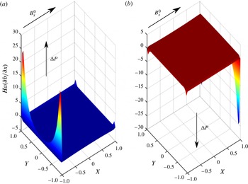
The precise mechanisms involved in these cases are worthy of further study. Figures 8 and 9 show the current distribution and the non-dimensional Lorentz force in the co-flow case, respectively. It is clear that the current density in the fluid at each of the Hartmann layers (and walls) is large and flows perpendicular to the applied field. Such currents give rise to steep gradients in the induced magnetic field within the Hartmann layers and correspondingly large non-dimensional Lorentz forces which act in the same direction as the pressure drop, as shown in figure 9. As a result, the net force is large in the Hartmann layer, giving rise to large shear stresses. The Lorentz forces are larger still in the corners near the connecting wall, with resulting increase in wall shear stress. Away from the walls, the non-dimensional Lorentz force reduces, ultimately opposing and balancing the pressure drop, resulting in the flat core region. The combination of these effects leads to the significant core flow in the co-flow case and enhanced core velocity near the adjoining wall (principally due to the corner effects). In the side walls, although the current is significant, it flows in a direction parallel to the induced field and the resulting Lorentz force is negligible. As a result, the side layer exhibits pressure driven flow, resulting in the observed jets. There is (relatively) weak coupling between the ducts due to the significant wall resistance along the current path in this configuration. This is, of course, dependent on the wall thickness and conductivity.
Electric current distribution for
 $\mathit{Ha}=500$
. Arrows represent the current flow, contours represent the magnitude of current density, co-flow case.

Non-dimensional Lorentz force for
 $\mathit{Ha}=500$
, co-flow, case: (a) duct 1; (b) duct 2.

In figure 10 is shown the current distribution in the counter-flow case. The current densities at the outer Hartmann layers are reduced relative to the co-flow case, particularly near the centre region of the wall, and less so near the corners. However, at the inner Hartmann walls, the current flows largely through the connecting wall, into the neighbouring duct. The connecting wall resistance is relatively low in this configuration, leading to strong coupling. The current near the inner Hartmann wall gives rise to greatly reduced non-dimensional Lorentz forces (figure 11) as it has a significant component parallel to the applied field. The component perpendicular to the applied field is similar in magnitude and direction to that in the core. As a result, the net force in the inner Hartmann layers is much smaller in this configuration, giving rise to negligible shear stresses. Away from the walls, the non-dimensional Lorentz force opposes and balances the pressure drop, again resulting in the flat core region. The combination of these effects leads to the greatly reduced core flow in the counter-flow case, resulting in an almost stagnant flow. In the side walls, as in the co-flow case, the resulting Lorentz force is negligible, giving rise to the observed pressure-driven jets.
Electric current distribution for
 $\mathit{Ha}=500$
. Arrows represent the current flow, contours represent the magnitude of current density, counter-flow case.

Non-dimensional Lorentz force for
 $\mathit{Ha}=500$
, counter-flow, case: (a) duct 1; (b) duct 2.
5.2. Triple ducts,
 $N=3$

For the case of three ducts, we consider in detail the co- and counter-flow cases. In the following we again choose the case where
 ${\it\delta}=0.02$
,
 ${\it\mu}_{f}={\it\mu}_{w}=1$
and
 ${\it\sigma}_{w}/{\it\sigma}_{f}=1$
, with each duct subject to a fixed pressure drop (in the appropriate directions).
The velocity profiles in the co-flow case are shown in figure 12(a). The peak and core flow velocities in the central duct (duct 2) are a little larger than those of the side ducts (ducts 1 and 3). The magnetic field, current flow and Lorentz force shown in figures 12(b), 13 and 14, respectively, are consistent with the twin duct case. The Lorentz forces are enhanced, particularly near the corners of the central duct, with a resulting increase in the velocity.
Velocity profile (a) and induced magnetic field (b) for
 $\mathit{Ha}=500$
, triple duct co-flow configuration.

Electric current distribution for
 $\mathit{Ha}=500$
. Arrows represent the current flow, contours represent the magnitude of current density, triple duct co-flow configuration.

Non-dimensional Lorentz force for
 $\mathit{Ha}=500$
, triple duct co-flow configuration: (a) duct 1 (side); (b) duct 2 (centre).

The velocity profiles in the counter-flow case are shown in figure 15(a). The peak and core flow velocities in the side duct (i) are strongly suppressed relative to the co-flow case. The core flow in the side duct is suppressed to approximately 20 % of the co-flow case, with a velocity
 ${\approx}-0.15$
. The core flow in the centre duct (ii) is not only suppressed, it is, in fact, reversed (relative to the applied pressure gradient). In this case, the core flow has a velocity
 ${\approx}-0.13$
. In the absence of a magnetic field (or indeed, the side ducts), a positive core flow would be expected.
Velocity profile (a) and induced magnetic field (b) for
 $\mathit{Ha}=500$
, triple duct counter-flow configuration.

The induced magnetic field is shown in figure 15(b). The current flow in this configuration is shown in figure 16 and it is worth noting that this differs markedly from the current flow in the twin duct counter-flow case (figure 10), where current flowed preferentially through the connecting wall (in the
 $x$
-direction). Due to the asymmetry between the side and centre ducts, there is in addition a significant current component along the wall (in the
 $y$
-direction), with concomitant enhancement of the Lorentz force near the connecting wall. The non-dimensional Lorentz force, shown in figure 17, is significantly reduced in the Hartmann layers in comparison to the co-flow case (by about a factor of 0.5). This leads to a reduction in wall shear stress and accounts for the reduction in core flow in the side duct. Notably, in the central duct, the coupling with the side ducts gives rise to a large Lorentz force in the Hartmann layers that act in opposition to the pressure drop (unlike the case for the side duct and all co-flow cases). This acts to further suppress the core flow in the central duct. If this near-wall Lorentz force is sufficiently large (due to a large Hartmann number and reduced wall resistance), then the core velocity can be entirely reversed, as is the case here. The side jets again correspond to regions of negligible Lorentz force and the jets result from pressure driven flow in the side layers and as a result do not experience flow reversal, hence flow in the duct is of a counter-current nature. Depending on the relative contributions to the mass flow rate of the core and side jets, it is possible to have a net reversal of the mass flow rate in the duct.
Electric current distribution for
 $\mathit{Ha}=50$
. Arrows represent the current flow, contours represent the magnitude of current density, triple duct counter-flow configuration.

Non-dimensional Lorentz force for
 $\mathit{Ha}=500$
, triple duct counter-flow configuration: (a) duct 1 (side); (b) duct 2 (centre).

So far in this section, we have fixed the Hartmann number, conductivities, permeabilities and wall thickness. The coupling effects are a function of these parameters. As stated earlier, for thin ducts, the dependence of the flow field can be characterized in terms of the conductivity ratio,
 $c_{w}$
. This is not the case for thick-walled ducts. In order to investigate the dependence of the coupling on these parameters, it is proposed to consider the total deviation from the single duct case across all ducts. To this end, the coupling parameter
 ${\it\alpha}$
is defined as
 $$\begin{eqnarray}{\it\alpha}=\mathop{\sum }_{i=1}^{N}\left|\frac{U_{m,i}}{U_{m}^{sh}}-{\rm\Delta}P_{i}\right|.\end{eqnarray}$$
Each term in this sum is the normalized difference between the mean velocity in the coupled case and the non-coupled case, for each duct. For a case with no coupling,
 ${\it\alpha}=0$
.
In figure 18 is shown the coupling parameter for the co- and counter-flow cases for
 $\mathit{Ha}=500$
as a function of
 ${\it\sigma}_{w}/{\it\sigma}_{f}$
and wall thickness
 ${\it\delta}$
. Both cases exhibit appropriate limiting behaviour for large
 ${\it\delta}$
and large
 ${\it\sigma}_{w}/{\it\sigma}_{f}$
, where the wall conductivity is large in comparison to the fluid conductivity. In this case the perfectly conducting wall case is approached and the coupling effects are negligible. It is also the case that the coupling decays rapidly for
 ${\it\delta}\gg 1$
.
Coupling parameter
 ${\it\alpha}$
as a function of
 ${\it\sigma}_{w}/{\it\sigma}_{f}$
and
 ${\it\delta}$
for
 $\mathit{Ha}=500$
: (a) co-flow case; (b) counter-flow case.

For the co-flow case (figure 18
a), in the limit of small
 ${\it\delta}$
and small
 ${\it\sigma}_{w}/{\it\sigma}_{f}$
, the perfectly insulating wall case is approached and again, coupling effects become negligible. For co-flow, current flows along the Hartmann walls, in the
 $y$
-direction (as shown in figure 13). In such circumstances, a wall conductance ratio,
 $c_{y}$
, can be characterized as
 $c_{y}\propto ({\it\sigma}_{w}{\it\delta})/({\it\sigma}_{f})$
. It is clear that for any given
 ${\it\delta}$
, the peak coupling occurs along a locus of points on which
 $c_{y}\propto ({\it\sigma}_{w}{\it\delta})/({\it\sigma}_{f})$
is constant, indicated by the white line in the figure. Whilst the figure shows a calculation for
 $\mathit{Ha}=500$
, increasing
 $\mathit{Ha}$
leaves the result qualitatively unchanged, but shifted to the left (in the direction of smaller
 ${\it\sigma}_{w}/{\it\sigma}_{f}$
), as indicated by the arrow. Conversely, decreasing
 $\mathit{Ha}$
shifts the values in the figure to the right. It is also to be noted that the peak value of the coupling parameter increases with increasing
 $\mathit{Ha}$
. As a result, for a given
 ${\it\delta}$
and
 ${\it\sigma}_{w}/{\it\sigma}_{f}$
, increasing
 $\mathit{Ha}$
leads to a rapid increase in coupling, reaching a peak, which then decays slowly.
For the counter-flow case (figure 18
b), current flows both through and along the Hartmann walls, as shown in figure 16. For current flowing through the wall (as opposed to along the wall), into the neighbouring duct, a wall conductance ratio is given by
 $c_{x}\propto ({\it\sigma}_{w})/({\it\sigma}_{f}{\it\delta})$
. Note that this conductance ratio will dominate the
 $c_{y}$
for
 ${\it\delta}<1$
. As
 ${\it\delta}$
is reduced, the conductance will increase and the coupling will be enhanced, irrespective of
 ${\it\sigma}_{w}/{\it\sigma}_{f}$
. Peak coupling occurs along a locus of points on which
 $c_{y}\propto ({\it\sigma}_{w})/({\it\sigma}_{f})$
is constant, indicated by the vertical white line in the figure. As with the co-flow case, increasing
 $\mathit{Ha}$
leaves the result qualitatively unchanged, but shifted to the left (in the direction of smaller
 ${\it\sigma}_{w}/{\it\sigma}_{f}$
), as indicated by the arrow. Conversely, decreasing
 $\mathit{Ha}$
shifts the values in the figure to the right. As in the co-flow case, for a given
 ${\it\delta}$
and
 ${\it\sigma}_{w}/{\it\sigma}_{f}$
, increasing
 $\mathit{Ha}$
leads to a rapid increase in coupling, reaching a peak, which then decays slowly. This strong coupling in the counter-flow case can lead to flow reversal of the core, to a point where the net flow is reversed, despite the side jets. The phenomenon of flow reversal is studied in figures 19–21, which indicate the mean velocity in the central duct as a function of
 ${\it\sigma}_{w}/{\it\sigma}_{f}$
and
 ${\it\delta}$
for
 $\mathit{Ha}=5,50$
and 500, respectively. No reversal of the mean velocity (corresponding to mean velocity
 $<0$
) is seen for
 $\mathit{Ha}=5$
, indeed, further investigation shows that net flow reversal occurs only for
 $\mathit{Ha}>13$
. For
 $\mathit{Ha}=50$
and 500, net flow reversal is clear.
Normalized central duct mean velocity as a function of
 ${\it\sigma}_{w}/{\it\sigma}_{f}$
and
 ${\it\delta}$
for
 $\mathit{Ha}=5$
, counter-flow case.

Normalized central duct mean velocity as a function of
 ${\it\sigma}_{w}/{\it\sigma}_{f}$
and
 ${\it\delta}$
for
 $\mathit{Ha}=50$
, counter-flow case.

Normalized central duct mean velocity as a function of
 ${\it\sigma}_{w}/{\it\sigma}_{f}$
and
 ${\it\delta}$
for
 $\mathit{Ha}=500$
, counter-flow case.

5.3. Multiple ducts,
$N=5$

The arrangement considered in this section consists of five ducts with
 ${\it\delta}=0.05$
in both co- and counter-flow configurations. Both fixed pressure drop and fixed mean velocity cases are considered. The effect of Hartmann number on the coupling between ducts is investigated.
For the case of a fixed pressure drop, an identical pressure drop is applied in each duct (differing only in sign in the counter-flow configuration). In figure 22(a) is shown the mean velocities (and fixed pressures) in each duct in the co-flow configuration, which indicates that there is flow enhancement relative to the single duct case, with the greatest enhancement in the central duct. As in the three duct case, the velocity and pressures are normalized with respect to the single duct case. The counter-flow case is shown in figure 22(b). The coupling between ducts has significant detrimental effects on the flow, with significantly reduced mean velocities in all ducts, especially ducts 2 and 4. Figures 23(a) (co-flow) and 23(b) (counter-flow) show the dependence of the normalized flow velocity on Hartmann number, for ducts 1, 2 and 3 (4 and 5 are identical to 2 and 1, respectively, due to symmetry).
Mean velocities in ducts with fixed pressure,
 $\mathit{Ha}=500$
: (a) co-flow case; (b) counter-flow case.

Mean velocities versus Hartmann number for fixed pressure drops: (a) co-flow case; (b) counter-flow case.

For the case of a fixed applied velocity, with the same arrangements as before, an identical mean velocity is applied in each duct (differing only in sign in the counter-flow configuration). The pressures (and fixed mean velocities) in each duct are shown in figure 24(a). As expected, for a given mean velocity, the necessary pressure drop is significantly reduced, which is to be expected. The counter-flow case is shown in figure 24(b). It is clear that pressure drops are increased by a factor of two to three relative to the single-duct case, in order to maintain the flow rates in this configuration. Figure 25(a) (co-flow) and (b) (counter-flow) show the dependence of the normalized flow velocity on Hartmann number, for ducts 1–3.
Pressure drop in ducts with fixed velocity,
 $\mathit{Ha}=500$
: (a) co-flow case; (b) counter-flow case.

Pressure drop versus Hartmann number with fixed velocities: (a) co-flow case; (b) counter-flow case.

It is clear from these results that the coupling between ducts in a co-flow configuration has beneficial effects in terms of pressure drop (or conversely mean velocity). However, it is also clear that these relative gains increase with increasing Hartmann number, only up to
 $\mathit{Ha}\sim 200$
. In the counter flow configurations, a similar behaviour is seen, albeit with a negative impact on hydrodynamic parameters. In these cases, pressure drops increase with increasing Hartmann number, reaching a peak at
 $\mathit{Ha}\sim 50$
, beyond which there is a reduction in the pressure drop relative to the single duct case.
The explanation of this dependence on Hartmann number can be viewed in the context of the coupling parameter shown in figure 18. Although figure 18 corresponds to a three-duct case, the results for the five-duct case are qualitatively similar. This five-duct case corresponds to a particular point in the plane of figure 18(a,b). For small
 $\mathit{Ha}$
, this point lies to the left of the peak loci. As
 $\mathit{Ha}$
increases, the loci move to the left, with coupling reaching a peak as the loci passes the point in the plane. As
 $\mathit{Ha}$
increases still further, the coupling diminishes (albeit relatively slowly, as explained in § 5.2).
6. Conclusion
This work presents an analytical solution to the laminar flow of an electrically conducting fluid in an array of partially conducting ducts of arbitrary wall thickness subject to an applied magnetic field. The solution is developed initially by applying the separation of variables method to the case of a single duct. The importance of considering the effect of arbitrary thickness walls on the flow is shown by demonstrating the limitations of the thin-wall approximation developed by Hunt. These results are then extended to arrays of two, three and five parallel ducts stacked in the direction of the applied magnetic field. The electromagnetic flow coupling between ducts and its impact on the flow is studied in detail, in both co- and counter-flow configurations. It is shown that the conducting walls have a strong influence on the currents near the walls and in particular on the Lorentz forces near the wall, giving rise to significant enhancement of shear stresses in the co-flow case which is beneficial in terms of pressure drop (or conversely mean velocity). In the counter-flow case there is strong suppression of wall shear stresses leading to a strong reduction of core flow. In certain circumstances, the coupling between ducts is sufficiently strong to induce flow reversal and counter-current flows result. Such phenomena are likely to have significant detrimental effects on both heat and mass transfer in fusion applications in particular. These analytical solutions give insight into the physics of such flows and provide important benchmarking and validation data for computational MHD, as well as approximate flow parameters for 1D systems codes.
Acknowledgements
We acknowledge the support of the Culham Centre for Fusion Energy (CCFE), Oxford, UK and Amec Foster Wheeler.
Appendix A. The Shercliff solution
The following Shercliff solution is valid for non-conducting walls, for a square duct of unit half-width.
 $$\begin{eqnarray}\displaystyle & U_{sh}(x,y)=\displaystyle \mathop{\sum }_{n=1}^{\infty }U_{n}(x)\cos {\it\lambda}_{n}y & \displaystyle\end{eqnarray}$$
 $$\begin{eqnarray}\displaystyle & B_{sh}(x,y)=\displaystyle \mathop{\sum }_{n=1}^{\infty }B_{n}(x)\cos {\it\lambda}_{n}y & \displaystyle\end{eqnarray}$$
 $$\begin{eqnarray}\displaystyle & U_{n}(x)=\displaystyle \frac{k_{n}}{{\it\lambda}_{n}^{2}}\left(1-\frac{\sinh p_{n_{2}}\cosh p_{n_{1}}x-\sinh p_{n_{1}}\cosh p_{n_{2}}x}{\sinh (p_{n_{2}}-p_{n_{1}})}\right) & \displaystyle\end{eqnarray}$$
 $$\begin{eqnarray}\displaystyle & B_{n}(x)=\displaystyle \frac{k_{n}}{{\it\lambda}_{n}^{2}}\left(\frac{\sinh p_{n_{1}}\sinh p_{n_{2}}x-\sinh p_{n_{2}}\sinh p_{n_{1}}x}{\sinh (p_{n_{2}}-p_{n_{1}})}\right) & \displaystyle\end{eqnarray}$$
 $$\begin{eqnarray}\displaystyle & p_{n_{1}}={\it\lambda}-\sqrt{{\it\lambda}^{2}+{\it\lambda}_{n}^{2}} & \displaystyle\end{eqnarray}$$
 $$\begin{eqnarray}\displaystyle & p_{n_{2}}={\it\lambda}+\sqrt{{\it\lambda}^{2}+{\it\lambda}_{n}^{2}} & \displaystyle\end{eqnarray}$$
 $$\begin{eqnarray}\displaystyle & {\it\lambda}_{n}=(n-{\textstyle \frac{1}{2}}){\rm\pi} & \displaystyle\end{eqnarray}$$
 $$\begin{eqnarray}\displaystyle & {\it\lambda}=\displaystyle \frac{\mathit{Ha}}{2} & \displaystyle\end{eqnarray}$$
 $$\begin{eqnarray}\displaystyle & k_{n}=\displaystyle 2\frac{\sin {\it\lambda}_{n}}{{\it\lambda}_{n}}. & \displaystyle\end{eqnarray}$$


 Open access

