


Introduction
The Greenland ice sheet is formed through snow deposition and can be viewed as an atmospheric sediment. the isotope ratio 18O/16O in the ice is a proxy for palaeotemperatures, while the dust concentration in the ice yields information about palaeowinds and source-area efficiency (see Reference Johnsen and AndersenJohnsen and others, 1997, and references therein). At the summit of the ice sheet, the ice flow is slow and vertical, and an undisturbed δ18O chronology for at least the last glacial cycle has been obtained through the Greenland Icecore Project (GRIP) (Reference DansgaardDansgaard and others, 1993) and Greenland Ice Sheet Project 2 (GISP2) (Reference Grootes, Stuiver, White, Johnsen and JouzelGrootes and others, 1993) deep ice cores. the finding of interrupted periods of a stadial and an interstadial climate suggests the existence of two quasi-stationary states between which the climate jumps, induced by fluctuations in the forcing. Model studies (Reference RahmstorfRahmstorf, 1995) show that high-resolution ocean models exhibit a bifurcation diagram similar to that found in simple box models of the type introduced by Reference StommelStommel (1961). the cause for the climate shifts in the models is destabilization of the quasi-stationary states caused by an external atmospheric forcing on the (North Atlantic) thermohaline circulation. Due to the internal fluctuations, transitions can be induced even though a full destabilization of the quasi-stationary states does not occur. In the case of a periodic external forcing, this can lead to stochastic resonance as has been proposed for the Dansgaard–Oeschger (D-O) events (Reference Alley, Anandakrishnan and JungAlley and others, 2001). In an ``intermediate-complexity’’ climate model, CLIMBER-2, Reference Ganopolski and RahmstorfGanopolski and Rahmstorf (2001) recently simulated the D-O events by forcing the model not quite to the bifurcation point for the onset of the D-O events, but such that the internal noise in the model induced a penetration of the reduced barrier. the model study suggests that the interstadial state is unstable, resulting in the gradual drift toward the stable stadial state.This is reflected in the sawtooth shape of the interstadial states.The ice-core data show that the gradual cooling of the interstadial states does not bring the state all the way to the stadial state. the terminations of the interstadial states are not gradual, but rapid like the terminations of the stadial states, as we will show later. This suggests a noise-induced penetration of a reduced barrier such that we will assume the existence of a quasi-stationary interstadial climate state in this analysis.
From a spectral analysis of the ice-core isotopic signal, the data can be interpreted as consisting of a slow climate component and a fast noise component (Reference Ditlevsen, Svensmark and JohnsenDitlevsen and others, 1996). In order to substantiate this, we have analyzed the two climate states separately and compared to the present climate variations as represented by the Holocene part of the ice-core record.
Separation of States
The stable-isotope record is shown later in Figure 2d and has been thoroughly discussed before (see Reference Johnsen and AndersenJohnsen and others, 1997, and references therein). the temporal resolution changes through the record, and for the glacial part of the record varies between 3 and 7 years.
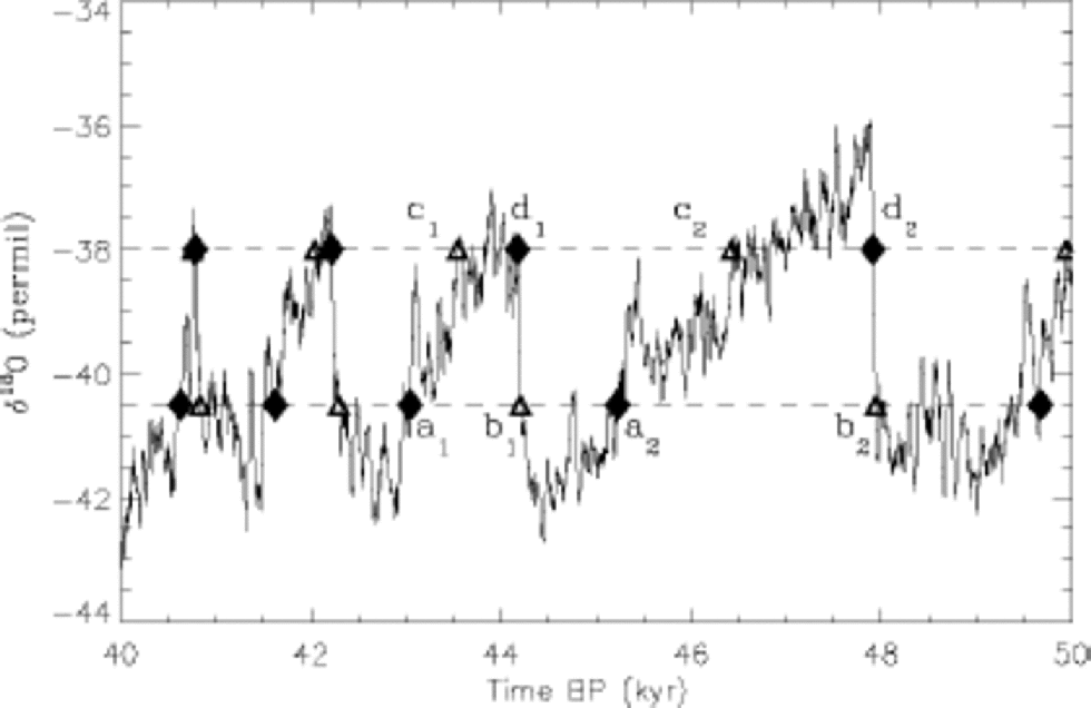
The separation into the two climate states is not completely straightforward since the fast fluctuations on top of the slow variations defining the separate states are quite significant. Here the separation has been done by identifying consecutive first up-crossings and down-crossings through two constant levels, δ18O = –38 per mil and δ18O = –40.5 per mil, of the 100 year running mean of the isotope record. A section of the record is shown in Figure 1. the dashed lines indicate the upper and lower levels. the point a1 is the first down-crossing point after the previous up-crossing point d1, both marked with diamonds. (Note that the plot follows the palaeoclimatic tradition of running backwards in time.) In this way we obtain the beginnings of the different regimes. the endings of the regimes are determined in the same way by moving backwards in time. Thus b1 is the first down-crossing point following an up-crossing c1, marked with triangles. This procedure makes the separations rather independent of the choices of the upper and lower levels, and separates the record into four regimes: the stadial, the interstadial and the two transitions stadial to interstadial and interstadial to stadial. Due to the characteristic sawtooth shapes of the isotope signal in the interstadial state, there are some ambiguities in determining the termination of the interstadials (the points marked ``c’’ in Fig. 1). However, the sawtooth shape of the interstadial states is not found in other ice-core parameters, such as the calcium ion concentration, so in principle we could find the determination from examining this record (Reference Fuhrer, Neftel, Anklin and MaggiFuhrer and others, 1993). This makes little difference to the present analysis. Here we define the stadial states as the periods between points of types ai+1 and bi while we define interstadials as periods in between points of types di and ai. (We lose too many data by using the periods between points of types di and ci to define the interstadials.) the sawtooth- shaped interstadials indicate a gradual drift toward the glacial state but with the characteristics, such as palaeowinds, of the interstadial climate preserved as indicated by the calcium ion concentration (Reference Fuhrer, Neftel, Anklin and MaggiFuhrer and others, 1993) and the variance of the isotope signal (Reference Johnsen and AndersenJohnsen and others, 1997) which shows no sign of a gradual drift toward the stadial state. the method employed here for separating the record into the different climatic states results in the same separation as that done ``by hand’’ by Reference DansgaardDansgaard and others (1993), represented by the numbering of the D-O states in Figure 2d.
The separation between stadial and interstadial states is done on the 20-point running average (variable time resolution) of the isotope signal. the periods are defined by the separation points being the first down-crossing time of a lower level (lower dashed line) after the signal has crossed up through an upper level (upper dashed line). This defines the points marked with a’s and d’s (diamonds). the b and c points (triangles) are obtained in the same way by moving backwards in time (from left to right in the plot). See text for further explanation.
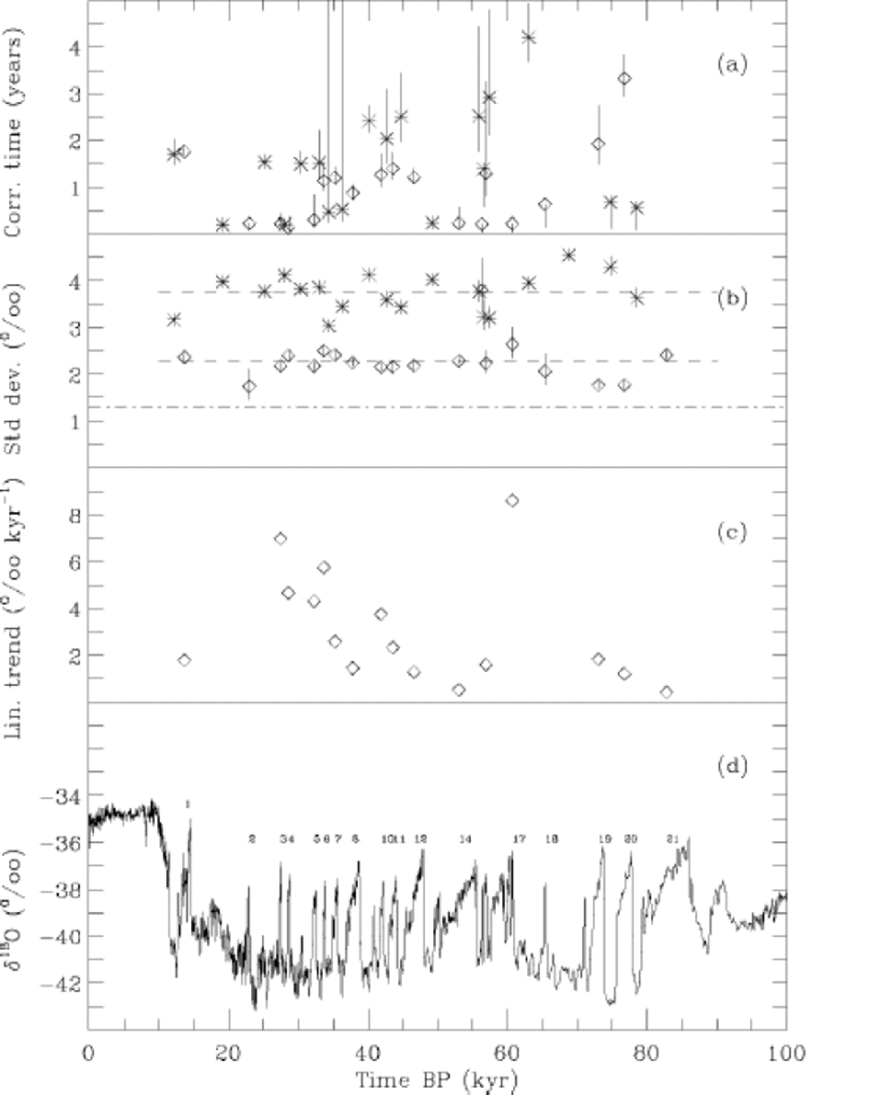
The δ18O signal from the GRIP ice core is separated into the stadial and interstadial states. for (a–c) the values calculated for the individual climatic periods are plotted as functions of the time period. (a) the correlation times are calculated using Equation (A4) in the Appendix for a likelihood estimate of the parameter α. (b) Standard deviation. the means for the stadial and interstadial states are shown by the upper and lower dashed lines, respectively. the dot-dashed line is the Holocene value. (c) Linear trends (the sawtooth) subtracted from the interstadials in order to make them stationary. (d) the 20-point average of the record. the numbering refers to the labelling by Reference DansgaardDansgaard and others (1993).
In order to analyze the statistics of the individual interstadial periods, we have subtracted the linear trend and thereby obtained stationary series. the ice core is dated using the ``ss09’’ time-scale (Reference JohnsenJohnsen and others, 1995).
Climate Dynamics
As a first approximation, the generic way of describing the variations on climatic time-scales is that each of the states can be described as resulting from a simple linear autoregressive process,

The δ18O climate variable is denoted xn, and the discrete time-steps are  where
 is the resolution of the record. the first term on the righthand side represents the ``stiffness’’ of the stable climate state in restoring the equilibrium state
 when the system is perturbed by noise. the second term on the righthand side is climatic noise which on these time-scales acts as a stochastic forcing. the intensity σ of the noise represents the strength of the atmospheric forcing on the climate state, and η is a unit variance white noise. the variance of the process can be calculated using Equation (1):
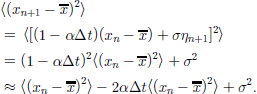
Here, η is taken to be a white noise, and the term of order  is neglected. Stationarity of the process requires the first term on the righthand side to equal the lefthand side (first line), and we obtain the fluctuation–dissipation theorem,

From observation of the variance  in the ice-core data, therefore, we cannot determine
 or α separately. We can determine α from the autocorrelation, assuming that Equation (1) describes the observed climate process. the autocorrelation for this process is obtained as

and by applying this i times we obtain

Here we use  in the limit
 so the process described by Equation (1) has an exponential autocorrelation. the absolute value in the exponent comes from the symmetry
 The correlation time is defined as

Analysis of the Isotope Climate Signal
Each separate record consists of samples giving average values from kyears, where k is the resolution at the given time. the glaciological noise unrelated to the climate signal in the annual isotope values is estimated by comparing shallow ice cores (Reference WhiteWhite and others, 1997). the amount of variance explained by the climate signal x is defined as  and thus
 This means that for k years averages, the amount of variance explained by the climate signal is
 since the glaciological noise has no temporal correlation. Thus for k >3 we have S >0.75. the glaciological noise arises mainly from discontinuous erosion or deposition at the surface (sastrugi). the minor effect from this noise on the several years average is thus to decrease the variance due to mixing, rather than to increase the variance.
Assuming that the record is generated by the process described in Equation (1), or rather the continuous version (Δt → 0) which is the Ornstein–Uhlenbeck process, we can estimate the correlation time in Equation (5) from the data. the ice-core data are measured as time averages of the underlying process:

where  The fact that the time intervals are varying through the record implies a slightly complicated estimator for the correlation time. Furthermore, the isotopes diffuse in the firn and, to a lesser degree, in the ice. This diffusion will increase the correlation time in the signal and must thus be taken into account when estimating the correlation time for the undisturbed signal. the diffusion length in the ice through the glacial ice younger than 60 kyr is around 1.6 cm, corresponding to around 1 year, thus removing the annual oscillation (Reference Johnsen and AndersenJohnsen and Andersen, 1997).
An estimator for the correlation time  is obtained using ``prediction-based estimating functions’’ (Reference SørensenSørensen, 2000; Ditlevsen and Sørensen, in press). the technique is somewhat more involved than the usual maximum-likelihood estimations, which cannot be applied to the isotope signal. the statistical method is described in the Appendix.
The calculated correlation times are shown in Figure 2a. the values for the stadials (stars) and interstadials (diamonds) are plotted with time as the abscissa. the error bars are obtained from an expression of the standard deviation ϵ for the estimate of α which is proportional to Ditlevsen and Sørensen, in press). the error-bar range is then given as
 The value for the Holocene part of the record cannot be obtained in a straightforward sense assuming the process described in Equation (1), because this part is dominated by the annual cycle, which is not included in Equation (1).
The standard deviations in the stadial and interstadial states, representing the climate variability, are shown in Figure 2b, plotted in the same way as Figure 2a.The error bars are the 90% confidence levels calculated from the χ2 distribution for variance of a Gaussian process. It is clearly seen that the level for the stadial states is higher than for the interstadials, in agreement withReference Johnsen and AndersenJohnsen and others (1997). the average values are indicated by the two dashed lines. the dot-dashed line is the value for the 0.1–7.5 kyr BP Holocene record.
Comparison With Present-Day Climate
The estimated correlation times vary somewhat through the glacial period (Fig. 2a). Part of the increase in correlation time before approximately 60 kyr canbe attributed to the diffusion of the signal not completely compensated in the analysis. In the period younger than 60 kyr, it seems that some periods show long correlation times of the order years, while others show correlation times of a few months. We do not at present know whether the surprisingly long correlation times in some, mainly glacial, periods are an artifact of noise in the isotope signal influencing the analysis or if they represent true climatic correlations. About half of the periods, both stadials and interstadials, show a correlation time of a few months, which is of the order expected for the proxy in the present climate. the long correlation times found in some of the periods are of the order of correlation times found in red-noise spectra observed in present-day instrumental records of sea-surface temperatures (SSTs) (Reference Frankignoul and HasselmannFrankignoul and Hasselmann, 1977) and El Niño indices (Reference Kestin, Karoly, Yano and Rayner.Kestin and others, 1998) which are of the order 3–5 years. the top part of the ice-core records from Summit, Greenland, do not correlate with the El Niño index or instrumental SST records. However, one could speculate that if the correlation times found represent a climate signal, there could be periods in the glacial climate when El Niño or other slowly varying oceanic signals are deposited in the isotope record. In terms of the simple model (Equation (1)), the longer correlation times mean that the climate was slower to react to perturbations of the equilibrium climate state because the restoring force was weaker.
The variance (the square of the standard deviation (Fig. 2b)) was significantly higher in the stadial than in the interstadials, when again it was higher than in the present Holocene climate. the intensity σ of the climate noise can now be obtained from the variances and the correlation times using Equation (3).
The noise intensity σ is related to the strength of the weather variability. the correlation time for atmospheric variables, such as surface temperatures, is of the order weeks (Reference WillebrandWillebrand, 1978), which is the time-scale of the baroclinic waves. the atmospheric forcing is thus effectively a white noise on climatic time-scales; the finding that the correlation time is of the same order for the stadial and interstadial periods indicates that the intensity of this atmospheric activity is stronger in the stadial climate than in the interstadial climate. This is in agreement with the finding of much stronger fluctuations in the calcium ion concentration during the stadials, because this concentration is interpreted as a sign of stronger atmospheric activity resulting in more uptake and transport of dust (Reference DitlevsenDitlevsen,1999). This substantiates the picture of stronger baroclinic activity in the stadial climate due to a larger extent of glaciers and sea ice and thus a stronger meridional temperature gradient in the mid-latitudes.
Linear Trends
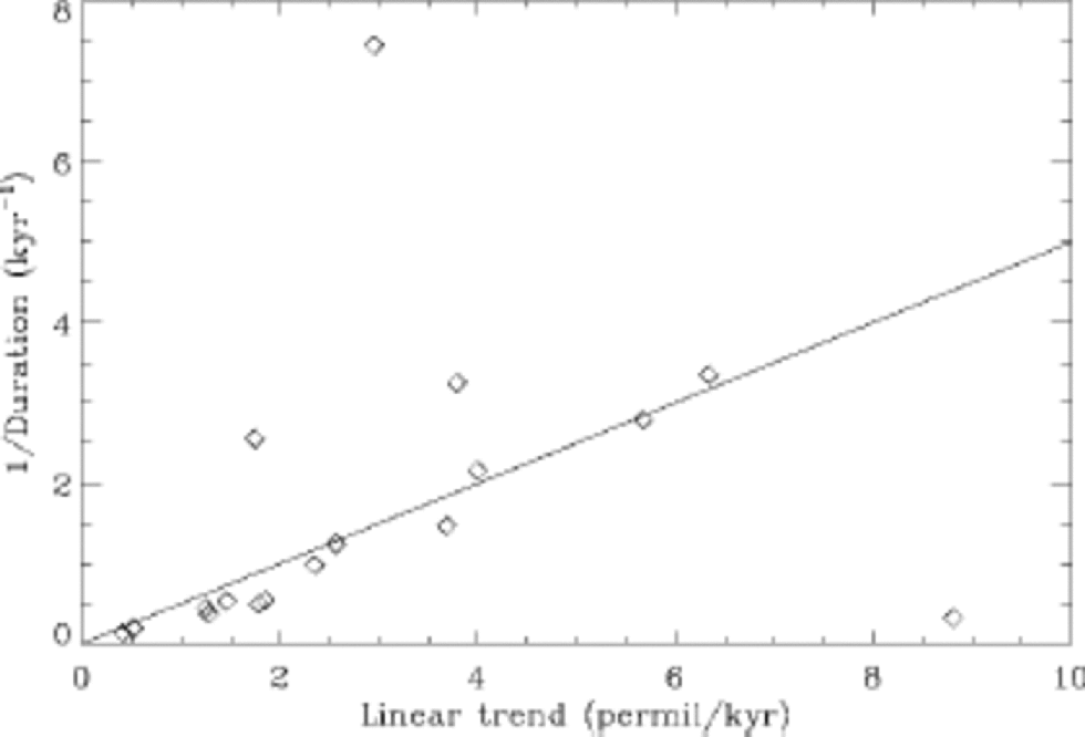
The linear trends subtracted from the interstadial states are plotted in Figure 2c. We do not at present know to what extent the gradual cooling represented by the sawtooth shape is a local phenomenon in Greenland. the rate of the gradual cooling is related to the duration of the interstadials (Reference Mogensen, Johnsen, Ganoploski and RahmstorfMogensen and Johnsen, 2002). the slope is correlated with the inverse of the duration of the interstadials (r = 0.64). the linear relation is (1/Duration)~ A–1 × (Linear Slope), where A = 2 per mil (see Fig. 3). Since the typical isotope values for the beginning of the interstadials are around –36 per mil and the values for the stadial states are around –40 per mil, only about half of the drop from the interstadial to the stadial states is explained by the gradual cooling. the other half is explained by a rapid transition. This indicates that the final transition to the stadial state is induced by a noise-driven penetration of a reduced barrier between quasi-stable states.
The linear relationship between the linear slope s (tendency) of the sawtooth-shaped interstadial states and 1/Δ, where Δ is the duration of the interstadials. the correlation coefficient is r = 0.64 and the relation is 1/Δ = A–1s ⇒ sΔ = A, where A = 2 per mil accounts for about half of the drop in isotopic value from the interstadial to the stadial state. This indicates that the interstadials are terminated by a rapid transition to the glacial state rather than through the gradual cooling represented by the linear slope.
Summary and Outlook
By inferring a simple auto-regressive model we can obtain a consistent picture of the variations within each of the two climate states and compare them with the present climate. the relatively large variations in the correlation times found in different periods call for a better understanding of the relation between the isotope proxy and the climate. the climate fluctuations resulting in the rapid shifts between the two quasi-stable states cannot be described by the linear stochastic dynamics (Equation (1)). the climate drift must be described by a non-linear model, where the two states correspond to steady states separated by a barrier. the penetration of the barrier is induced by the noise. the waiting time for penetration depends on the intensity of the noise and the height of the barrier. Work is in progress on extending this analysis to a non-linear stochastic model with statistical properties similar to the isotope signal. Simulating the palaeoclimate data in terms of non-linear stochastic models serves as a benchmark for more realistic climate modelling of the glacial climate.
Acknowledgements
Discussions with S. Johnsen were greatly appreciated. We are grateful for comments from an anonymous reviewer which led to significant improvements in the manuscript. K.K.A. thanks the Carlsberg Foundation for funding.
Appendix
The continuous version of the process described by Equation (1) is the stationary Ornstein–Uhlenbeck process:

When Equation (A1) is assumed to generate an observed data series, we can estimate the parameters (σ,σ) from the data by maximizing the likelihood function with respect to the parameters. the likelihood function L(x1,x2, ...; θ1, θ2, ...) is simply the product of the probabilities of obtaining each of the observed data xi given the parameters θ1, θ2, ... .The maximum is obtained by differentiating the likelihood function or the logarithm of the likelihood function (loglikelihood function) with respect to the parameters. the derivative G(x,θ)= ∂θ logL(x, θ) of the loglikelihood function or the likelihood function is called the score function. Themaximum likelihood obtained from G(x,θ) = 0 then gives the parameters θ for which the observed data are most likely. If the observed data were directly given by Equation (A1) we would have an explicit expression for the probabilities and thus the likelihood function. However, since the isotopic data are obtained as averages over non-equidistant periods and furthermore subject to diffusion and glaciological noise, the likelihood function is not explicitly available. Here we apply ``prediction-based estimating functions’’ (Reference SørensenSørensen, 2000; Ditlevsen and Sørensen, in press), which are an extension of ``martingale estimating functions’’. Martingale estimating functions utilize the fact that both the underlying process and the discrete data records are Markov processes. the idea is to approximate the unknown score function, that is, the differentiated loglikelihood function. An estimator is found by setting the estimating function to 0 and solving for the parameter. the unknown underlying process has the autocorrelation function  We are interested in estimating α which is the inverse of the correlation time. the ice-core data are not discretely observed, but averages of the underlying process over time intervals:

where Δi = ti -ti–1, and Zs is the diffused isotope signal.
We are no longer observing a Markov process, which implies that we cannot use martingale estimating functions for the inference problem. So we use prediction-based estimating functions, which are a generalization of martingale estimating functions. These are based on predictors of functions of the observed process, and are constructed by means of moments of the process. Not considering that we are observing averages would cause us to underestimate α and thus overestimate the correlation time.
The diffusion in the ice results in a further smoothing of the data. for simplicity we will treat the diffusion as resulting in a running average over the effective diffusion time λ (Reference Johnsen and AndersenJohnsen and Andersen, 1997). We thus simply assume,

where X is the undisturbed signal.
Then our estimating function will have the following form:
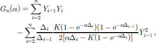
where

and our estimator  will be such that

The variance of the estimator used for the error bars in the estimated correlation times can be found by means of methods described in Reference SørensenSørensen (2000).



