1. Introduction
The development of methods and investigation of phenomena leading to the reduction of skin friction drag in turbulent flows has been an active area of research for several decades, and different strategies have been proposed and studied with mixed success. Of these, superhydrophobic surfaces for naval applications have received a great deal of attention recently. Superhydrophobicity enables textured surfaces immersed in water to entrap pockets (or bubbles) of air. The bubbles can lodge within the texture grooves, when the groove size is small enough. This is known as the Cassie–Baxter state (Cassie & Baxter Reference Cassie and Baxter1944), in opposition to the fully wetted, Wenzel state (Wenzel Reference Wenzel1936), in which the surface cavities are filled with water and the hydrophobic effect is diffused away. Under Cassie–Baxter conditions, much of the overlying water flow is in contact with the entrapped air, and not with the solid surface. Thus, the air ‘layer’ acts as a lubricant for the outer flow, which can effectively slip over the wall, experiencing reduced friction compared to conventional, smooth surfaces (Rothstein Reference Rothstein2010). The drag-reducing properties of superhydrophobic surfaces were first demonstrated for laminar flows (Watanabe, Yanuar & Udagawa Reference Watanabe and Udagawa1999; Ou, Perot & Rothstein Reference Ou, Perot and Rothstein2004; Choi & Kim Reference Choi and Kim2006; Choi et al. Reference Choi, Ulmanella, Kim, Ho and Kim2006). Under turbulent conditions, Daniello, Waterhouse & Rothstein (Reference Daniello, Waterhouse and Rothstein2009) showed experimentally that superhydrophobic surfaces were able to achieve high drag reductions of more than 25 %. Min & Kim (Reference Min and Kim2004) studied the reduction for turbulent flows numerically, by modelling the effective hydrophobicity as a spatially uniform slip length. They also studied the effect of these surfaces on the stability of the flow and the transition to turbulence (Min & Kim Reference Min and Kim2005). Their assumption of a single, homogeneous slip length, analogous to the nanoscale Navier-slip effect of hydrophobicity (Thompson & Troian Reference Thompson and Troian1997; Freund Reference Freund2003), implies that the surface texture modelled is isotropic. More recently, Busse & Sandham (Reference Busse and Sandham2012) comprehensively investigated the effects of slip length anisotropy on turbulence statistics. The detailed geometry of the texture was first studied in simulations by Martell, Perot & Rothstein (Reference Martell, Perot and Rothstein2009), who used a patterned slip/no-slip boundary condition to model the alternating contact with the entrapped air pockets and the roughness crests separating them.
Although the drag-reducing properties of superhydrophobic surfaces on turbulent flows have received a great deal of attention, both experimentally (Daniello et al. Reference Daniello, Waterhouse and Rothstein2009; Woolford et al. Reference Woolford, Prince, Maynes and Webb2009; Bidkar et al. Reference Bidkar, Leblanc, Kulkarni, Bahadur, Ceccio and Perlin2014; Park, Sun & Kim Reference Park, Sun and Kim2014; Srinivasan et al. Reference Srinivasan, Kleingartner, Gilbert, Cohen, Milne and McKinley2015) and numerically (Min & Kim Reference Min and Kim2004; Martell et al. Reference Martell, Perot and Rothstein2009; Martell, Rothstein & Perot Reference Martell, Rothstein and Perot2010; Park, Park & Kim Reference Park, Park and Kim2013; Jelly, Jung & Zaki Reference Jelly, Jung and Zaki2014; Türk et al. Reference Türk, Daschiel, Stroh, Hasegawa and Frohnapfel2014), the interaction of these surfaces with the flow has not yet been fully investigated. The above cited numerical studies, for instance, have concentrated on the drag-reducing slip effect, without considering the problem of gas–liquid interface stability and bubble depletion. The drag reduction predicted by these studies increases with the size of the texture grooves, in agreement with the theoretical analyses of Lauga & Stone (Reference Lauga and Stone2003), Fukagata, Kasagi & Koumoutsakos (Reference Fukagata, Kasagi and Koumoutsakos2006), Ybert, Barentin & Cottin-Bizonne (Reference Ybert, Barentin and Cottin-Bizonne2007) and Belyaev & Vinogradova (Reference Belyaev and Vinogradova2010), although the behaviour deviates from the theoretical linear predictions for large textures. In real flows, however, the Cassie–Baxter state, and thus drag reduction, is completely lost for textures larger than a threshold size (Aljallis et al. Reference Aljallis, Sarshar, Datla, Sikka and Jone2013; Bidkar et al. Reference Bidkar, Leblanc, Kulkarni, Bahadur, Ceccio and Perlin2014). Therefore, the development of insights that can lead to optimal design of superhydrophobic textures requires advancement of knowledge of flow–interface interactions, and a mechanism of interface breakage when these surfaces are subject to turbulent flow conditions.
In this paper, we present the first investigation of such mechanisms by studying the pressure loads on the air–water interface. We intend to establish a clear distinction between the dynamical mechanisms related to the size of the texture and those related to the overlying flow being turbulent. We analyse with special emphasis the different scalings for both types of mechanisms. The purpose of such study is twofold.
First, we assess the validity of extrapolating the conclusions of numerical simulations to practical flows. Most experimental measurements reported, like those of Daniello et al. (Reference Daniello, Waterhouse and Rothstein2009) and Park et al. (Reference Park, Sun and Kim2014), have been conducted at texture sizes of order
 $L^{+}\approx 0.5$
–
 $5$
, where the ‘
 $+$
’ superscript denotes scaling with the kinematic viscosity
 ${\it\nu}$
and the friction velocity
 $u_{{\it\tau}}$
. Although no clear reason has been given, it is likely that for larger textures the stability of the bubbles is lost, since they would otherwise yield larger drag reductions. In contrast, most of the numerical studies cited above have been conducted at
 $L^{+}\approx 10$
–
 $200$
, and most often near the upper limit. This is frequently due to a compromise between computational cost and physical fidelity. However, these numerical simulations assume a stable and flat air–water interface, but it is unclear whether a gas layer would remain stable at such large
 $L^{+}$
. It is also questionable whether some of the dynamics that are reported in the large
 $L^{+}$
range would be relevant at the smaller
 $L^{+}$
values of real applications.
Second, we characterize deleterious effects that appear as
 $L^{+}$
increases, leading to the degradation of the improving-with-size performance, and eventually to the complete loss of the superhydrophobic effect. Some work in this direction has begun to appear recently, but the mechanisms implicated in the degradation are still largely unknown. Steinberger et al. (Reference Steinberger, cile Cottin-Bizonne, Kleimann and Charlaix2007), Hyväluoma & Harting (Reference Hyväluoma and Harting2008), Teo & Khoo (Reference Teo and Khoo2010) and Karatay et al. (Reference Karatay, Haase, Visser, Sun, Lohse, Tsaia and Lammertink2013) have studied the effect of bubble shape when the interface is not perfectly flat, while Busse & Sandham (Reference Busse and Sandham2013) have analysed how the performance degrades as the height of the air layer decreases, and the texture crests begin to protrude out of it, introducing a roughness-like effect. Lee & Kim (Reference Lee and Kim2009), Patankar (Reference Patankar2010) and Samaha, Vahedi & Gad-el-Hak (Reference Samaha, Vahedi and Gad-el-Hak2011) have analysed the transition from the Cassie–Baxter to the Wenzel state through static pressure effects. Aljallis et al. (Reference Aljallis, Sarshar, Datla, Sikka and Jone2013) have experimentally considered the effect of shear on bubble depletion at high Reynolds numbers. Bidkar et al. (Reference Bidkar, Leblanc, Kulkarni, Bahadur, Ceccio and Perlin2014) examined different types of surface coating, changing chemical treatment and surface roughness size, and suggested that, for stable drag reduction at high Reynolds numbers, the roughness height should be much smaller than the viscous sublayer. Here we investigate the modulation with texture size of the pressure forces that act on the bubbles. As these forces increase with the texture size, they impose an upper limit on the possible texture dimensions, since for larger textures the air–water interface is not able to withstand the pressure forces for a given finite surface tension. The pressure stresses on the interface may on their own be a direct cause of the interface instability as the texture size increases.
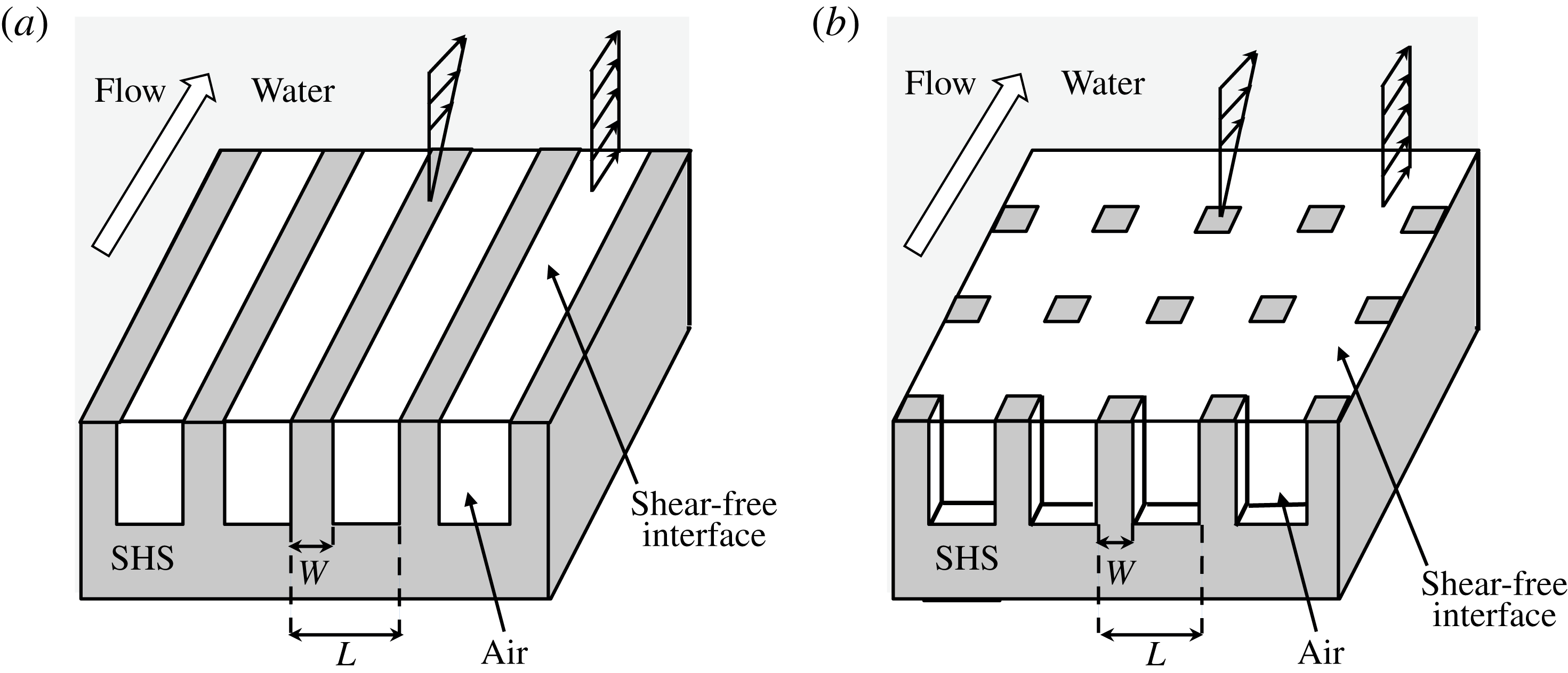
In direct relation to those pressure stresses, we study two types of geometrical patterns: two-dimensional ones aligned in the direction of the flow, or ridges, and three-dimensional ones equally distributed along the streamwise and spanwise directions, or posts. A schematic diagram of these geometries is shown in figure 1. Streamwise ridges have often been favoured in experiments, while the posts would, according to the theoretical predictions, yield larger drag reductions for the same feature width. We will see that posts are more sensitive to pressure stresses as
 $L^{+}$
increases. This may be a reason for choosing ridges when aiming to maximize the texture spacing, so the stability of the gas pockets is maintained. Nevertheless, studying the three-dimensional post geometry is likely more relevant to practical applications, since most economically feasible methods of fabrication of superhydrophobic surfaces involve spraying of material or similar processes that result in the protrusion of post-like geometries on the surface, as opposed to streamwise structures.
Schematic representation of a channel with superhydrophobic-surface boundary conditions on both walls, (a) streamwise-aligned ridges and (b) posts. Note that these representations do not exactly portray the arrangements studied, which have more texture features in the simulation domain than shown here.

The paper is organized as follows. In § 2 we present the equations and discuss the key dimensions and dimensionless parameters for the problem. In § 3 we outline the algorithms used to numerically solve that set of equations. The results of our simulations are presented and discussed in § 4. Finally, our conclusions are summarized in § 5.
2. Problem formulation
We consider the motion of a turbulent liquid flow in a doubly periodic channel with superhydrophobic rough walls that have entrapped gas pockets, as sketched in figure 1. The roughness consists of a streamwise- and/or spanwise-periodic patterned texture of period
 $L$
. We assume that the flow is governed by the incompressible Navier–Stokes equations,
 $$\begin{eqnarray}\displaystyle & \displaystyle \boldsymbol{{\rm\nabla}}\boldsymbol{\cdot }\boldsymbol{u}=0, & \displaystyle\end{eqnarray}$$
 $$\begin{eqnarray}\displaystyle & \displaystyle \frac{\partial \boldsymbol{u}}{\partial t}+\boldsymbol{u}\boldsymbol{\cdot }\boldsymbol{{\rm\nabla}}\boldsymbol{u}=-\boldsymbol{{\rm\nabla}}p+{\it\nu}{\rm\nabla}^{2}\boldsymbol{u}, & \displaystyle\end{eqnarray}$$
 ${\it\nu}$
is the kinematic viscosity and the liquid density is
 ${\it\rho}=1$
.
The flow is bounded by protruding patterned elements and the gas pockets interspersed between them. No slip is assumed at the solid–liquid interfaces, and the air/water viscosity ratio is considered to be small enough that the gas–liquid interface can be modelled by a free-slip boundary condition. All the boundaries are impermeable, and we neglect the deformation of the gas–liquid interfaces in the simulations of the flow. This is the standard treatment in the literature for DNS considering superhydrophobic textures (Min & Kim Reference Min and Kim2004; Martell et al. Reference Martell, Perot and Rothstein2009, Reference Martell, Rothstein and Perot2010; Busse & Sandham Reference Busse and Sandham2013; Park et al. Reference Park, Park and Kim2013; Jelly et al. Reference Jelly, Jung and Zaki2014; Türk et al. Reference Türk, Daschiel, Stroh, Hasegawa and Frohnapfel2014). However, a posteriori, we calculate the deformation of the interface responding to the pressure difference from the DNS results, as an equivalent way of representing the pressure distribution on the wall. The deformation of the interface obeys the Young–Laplace equation,
 $$\begin{eqnarray}{\rm\nabla}^{2}{\it\eta}\approx \frac{P_{liquid}-P_{gas}}{{\it\sigma}},\end{eqnarray}$$
where
 ${\it\sigma}$
is the surface tension and
 ${\it\eta}$
is the interface height measured from the channel wall plane at
 $y^{+}=0$
. Within the gas pockets, we assume
 $P_{gas}$
is uniform and governed by the mass conservation of the gas,
 $$\begin{eqnarray}\iint {\it\eta}\,\text{d}x\,\text{d}z=0.\end{eqnarray}$$
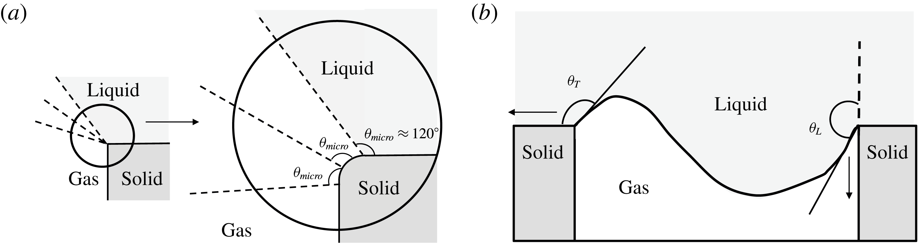
The gas–liquid interface is assumed to be effectively pinned to the post edges, as shown in figure 2(a), which are macroscopically sharp but can be rounded on a microscopic scale. The microscopic contact angle,
 ${\it\theta}_{\mathit{micro}}$
, can stay unchanged (or in between the nominal advancing and receding contact angles) while the macroscopic corner angles,
 ${\it\theta}_{T}$
and
 ${\it\theta}_{L},$
may be altered and allowed to adjust their contact point along the round corner. This assumption, together with the mass conservation of the gas, implies that the interface is never broken and the air bubbles are stably pinned inside the roughness. This assumption is reasonable as long as
 ${\it\theta}_{rec}-{\rm\pi}/2<{\it\theta}_{L}<{\it\theta}_{adv}$
and
 ${\it\theta}_{rec}<{\it\theta}_{T}<{\it\theta}_{adv}+{\rm\pi}/2$
, where
 ${\it\theta}_{adv}$
and
 ${\it\theta}_{rec}$
are the microscopic advancing and receding contact angles respectively. Moreover, we will use such a framework to predict the onset conditions leading to interface breakage.
(a) Macroscopic corner angle and microscopic contact angles under the pinned interface assumption. (b) Corner angles at the trailing edge (
 ${\it\theta}_{T}$
) and leading edge (
 ${\it\theta}_{L}$
).

The dimensional analysis of the problem reveals that the solution depends on a number of dimensionless parameters. The first is a Reynolds number based on the channel half-height, for instance the friction Reynolds number
 $\mathit{Re}_{{\it\tau}}=u_{{\it\tau}}{\it\delta}/{\it\nu}$
, which measures how ‘turbulent’ the flow is. For a realistic naval application with a moving object of dimensions of order
 ${\sim}1~\text{m}$
and a velocity of order
 ${\sim}5~\text{m}~\text{s}^{-1}$
,
 $\mathit{Re}_{{\it\tau}}$
is typically
 ${\sim}4000$
. This value is at present barely reachable by direct numerical simulation, even for smooth walls (Lozano-Durán & Jiménez Reference Lozano-Durán and Jiménez2014; Lee & Moser Reference Lee and Moser2015). Instead, we run our simulations at more modest
 $\mathit{Re}_{{\it\tau}}\approx 200{-}400$
, at which near-wall effects can still be correctly simulated (García-Mayoral & Jiménez Reference García-Mayoral and Jiménez2012) at a more cost-effective expense.
Another important Reynolds number is the size of the texture in viscous units,
 $L^{+}=u_{{\it\tau}}L/{\it\nu}$
, which measures how much the flow deviates from a canonical, smooth-wall flow. For small
 $L^{+}$
, the effect of the superhydrophobic surface can be treated as a perturbation for the buffer layer flow, while for large
 $L^{+}$
the flow is completely modified and resembles more a flow around obstacles (Jiménez Reference Jiménez2004). As mentioned above, typical experimental values are
 $L^{+}\lesssim 5$
. In the present work, we have investigated textures with sizes
 $L^{+}\approx 6{-}155$
. Our smallest surface wavelength can be applicable for the recent experimental studies and reaches the practical limit. Previous numerical studies have used
 $L^{+}$
values of the order of a hundred (Martell et al.
Reference Martell, Perot and Rothstein2009, Reference Martell, Rothstein and Perot2010; Busse & Sandham Reference Busse and Sandham2013; Jelly et al.
Reference Jelly, Jung and Zaki2014; Türk et al.
Reference Türk, Daschiel, Stroh, Hasegawa and Frohnapfel2014). In spite of the large slip velocities and drag reductions that they produce, such predictions are practically unrealistic since they do not incorporate considerations of gas layer stability. The underlying reason is again that the resolution required for the simulation of smaller textures makes them very expensive, and such simulations are only beginning to appear (Türk et al.
Reference Türk, Daschiel, Stroh, Hasegawa and Frohnapfel2014). Results obtained at
 $L^{+}\approx 100{-}150$
should be treated with caution, and only for the purpose of qualitative analysis.
The third dimensionless parameter involves the air–water interfacial surface tension. We follow the convention introduced by Seo, García-Mayoral & Mani (Reference Seo, García-Mayoral and Mani2013) and introduce the Weber number,
 $\mathit{We}^{+}={\it\rho}u_{{\it\tau}}{\it\nu}/{\it\sigma}$
, where
 ${\it\sigma}$
represents the surface tension. We should note that the Weber number that is naturally relevant to interface breakage should involve
 $L^{+}$
and slip velocity (which is not known a priori). However, the adopted
 $\mathit{We}^{+}$
makes the subsequent scaling analysis of interface deformation easier since it remains unchanged when we change the texture size,
 $L^{+}$
.
In this study, we consider values for
 $\mathit{We}^{+}$
corresponding to practical applications. For a water density of
 $1000~\text{kg}~\text{m}^{-3}$
, a surface tension of
 $0.073~\text{N m}^{-1}$
and a typical boundary layer velocity of
 $U_{\infty }=6{-}10~\text{m}~\text{s}^{-1}$
over a plate 0.5–10 m long, the values would be in the range
 $\mathit{We}^{+}=10^{-3}{-}10^{-2}$
.
3. Numerical method
The three-dimensional Navier–Stokes equations are discretized and solved computationally with the code of Bose, Moin & You (Reference Bose, Moin and You2010), adapted to treat DNS of superhydrophobic textured boundaries. The code uses a second-order finite-difference scheme on a staggered mesh (Morinishi et al.
Reference Morinishi, Lund, Vasilyev and Moin1998). The grid is Cartesian with uniform spacing in the streamwise (
 $x$
) and spanwise (
 $z$
) directions, and stretching in the wall-normal (
 $y$
) direction. The time discretization uses a second-order Adams–Bashforth scheme for the nonlinear and wall-parallel diffusion terms, and a second-order Crank–Nicholson scheme for the wall-normal diffusion terms. Incompressibility is imposed through a fractional step implementation (Kim & Moin Reference Kim and Moin1985). The computational domain is a periodic channel of ratio length–width–height of
 $2{\rm\pi}\times {\rm\pi}\times 2$
, standard for simulations that focus on near-wall effects (Martell et al.
Reference Martell, Perot and Rothstein2009, Reference Martell, Rothstein and Perot2010; García-Mayoral & Jiménez Reference García-Mayoral and Jiménez2012). The flow is driven by a time-constant mean pressure gradient, so that
 $\mathit{Re}_{{\it\tau}}$
is fixed. The main set of simulations is conducted at
 $\mathit{Re}_{{\it\tau}}\approx 200$
, with two simulations at
 $\mathit{Re}_{{\it\tau}}\approx 400$
to investigate Reynolds-number effects.
The time integration is conducted using a constant Courant–Friedrichs–Lewy number,
 $\text{CFL}=0.25$
, so that the variable time step is determined by
 $$\begin{eqnarray}{\rm\Delta}t=\text{CFL}\times \left(\max \left\{\frac{|u|}{2{\rm\Delta}x}+\frac{|v|}{2{\rm\Delta}y}+\frac{|w|}{2{\rm\Delta}z}+\frac{4}{\mathit{Re}{\rm\Delta}x^{2}}+\frac{4}{\mathit{Re}{\rm\Delta}z^{2}}\right\}\right)^{-1}.\end{eqnarray}$$
The simulations were run for at least 35 largest-eddy-turnover times
 ${\it\delta}/u_{{\it\tau}}$
, of which the first 10 were discarded for statistical sampling, to avoid any contamination from initial transients.
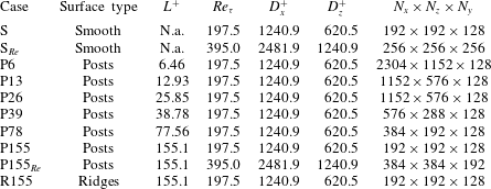
Simulation parameters.
 $L^{+}$
is the pattern spacing and
 $\mathit{Re}_{{\it\tau}}$
is the friction Reynolds number. The domain size for streamwise and spanwise directions is
 $D_{x}^{+}$
and
 $D_{z}^{+}$
. The spatial resolution is given by
 $N_{x}$
,
 $N_{z}$
and
 $N_{y}$
, the number of grid points for streamwise, spanwise and wall-normal directions.

All simulations use symmetric channels, with both walls being either smooth or superhydrophobic. In the latter case, the gas–liquid interface is modelled as a perfect-slip boundary condition, resulting in a pattern of slip and no-slip conditions (Martell et al.
Reference Martell, Perot and Rothstein2009). We study the patterns sketched in figure 1(a), streamwise-aligned ridges, and figure 1(b), posts distributed uniformly in the streamwise (
 $x$
) and spanwise (
 $z$
) directions. Spanwise-aligned ridges are less efficient for drag reduction than streamwise-aligned ones (Min & Kim Reference Min and Kim2004; Choi et al.
Reference Choi, Ulmanella, Kim, Ho and Kim2006; Martell et al.
Reference Martell, Perot and Rothstein2009), and thus we have not considered them in our study. The pattern thickness is set to
 $W=L/3$
, so the solid fraction is
 $1/9$
for posts and
 $1/3$
for ridges.
In the wall-normal direction, the stretched grid has
 $\min ({\rm\Delta}y^{+})=0.15$
at the wall and
 $\max ({\rm\Delta}y^{+})=12$
at the centre of the channel. The
 $x$
and
 $z$
spatial resolution is determined by the texture size, so that the number of points per texture unit
 $n_{x}$
,
 $n_{z}$
is sufficient to resolve the mean texture properties (e.g.
 $U_{s}^{+}$
,
 $p_{\mathit{rms},y=0}^{\prime +}$
). The parameters of the simulations are summarized in table 1. Even for the largest textures, this resolution is finer than that required for DNS of turbulence, with
 ${\rm\Delta}x^{+}=6.4$
,
 ${\rm\Delta}z^{+}=3.2$
at most. However, detailed pressure distributions near posts need further attention, due to the singularity at the post edge facing the streamwise slipping flow, where the patterned slip/no-slip boundary condition is analogous to the boundary layer over a sharp corner (Van Dyke Reference Van Dyke1962). This singularity gives rise to resolution-dependent values of the pressure at the edge. Nevertheless, given the nature of (2.3), and the pinned boundary condition for the air–water interface, the corner singularity still leads to a regular solution for the interface deformation. As a result, we have been able to establish grid-converged results for interface and pressure fields away from corners with the adopted resolutions.
The code was validated with the turbulent, smooth-wall channel at
 $\mathit{Re}_{{\it\tau}}\approx 395$
of Moser, Kim & Mansour (Reference Moser, Kim and Mansour1998), and the superhydrophobic channels with streamwise ridges of gas fraction
 $1/2$
and size
 $L^{+}\approx 74$
and
 $148$
, also at
 $Re_{{\it\tau}}\approx 395$
, from Martell et al. (Reference Martell, Rothstein and Perot2010). Resolution tests were run for case P155 with
 $n_{x}=48$
,
 $n_{z}=96$
and
 $n_{x}=72$
,
 $n_{z}=144$
, and results showed grid convergence, as shown in figure 3. To assess the validity of the grid resolution in the small-texture limit, a resolution test for P26 was also run at
 $n_{x}=n_{z}=12$
, and the two grid resolutions are also in excellent agreement, as shown in figure 4. The mean slip velocity of P155 has an error of the coarsest case to the finest case below 1 %, and all other cases had a smaller convergence error.
Resolution test for the post geometry with
 $L^{+}\approx 155$
at
 $Re_{{\it\tau}}\approx 200$
. (a) Mean streamwise velocity profile; (b) velocity r.m.s. fluctuations; (c) pressure r.m.s. fluctuations.

 ${\rm\Delta}x^{+}\approx 6.4$
,
 ${\rm\Delta}z^{+}\approx 3.2$
;

 ${\rm\Delta}x^{+}\approx 3.2$
,
 ${\rm\Delta}z^{+}\approx 1.6$
;

 ${\rm\Delta}x^{+}\approx 2.2$
,
 ${\rm\Delta}z^{+}\approx 1.1$
.

Resolution test for the post geometry with
 $L^{+}\approx 26$
at
 $Re_{{\it\tau}}\approx 200$
. (a) Mean streamwise velocity profile; (b) velocity r.m.s. fluctuations; (c) pressure r.m.s. fluctuations;

 ${\rm\Delta}x^{+}={\rm\Delta}z^{+}\approx 2.2$
;

 ${\rm\Delta}x^{+}={\rm\Delta}z^{+}\approx 1.1$
.

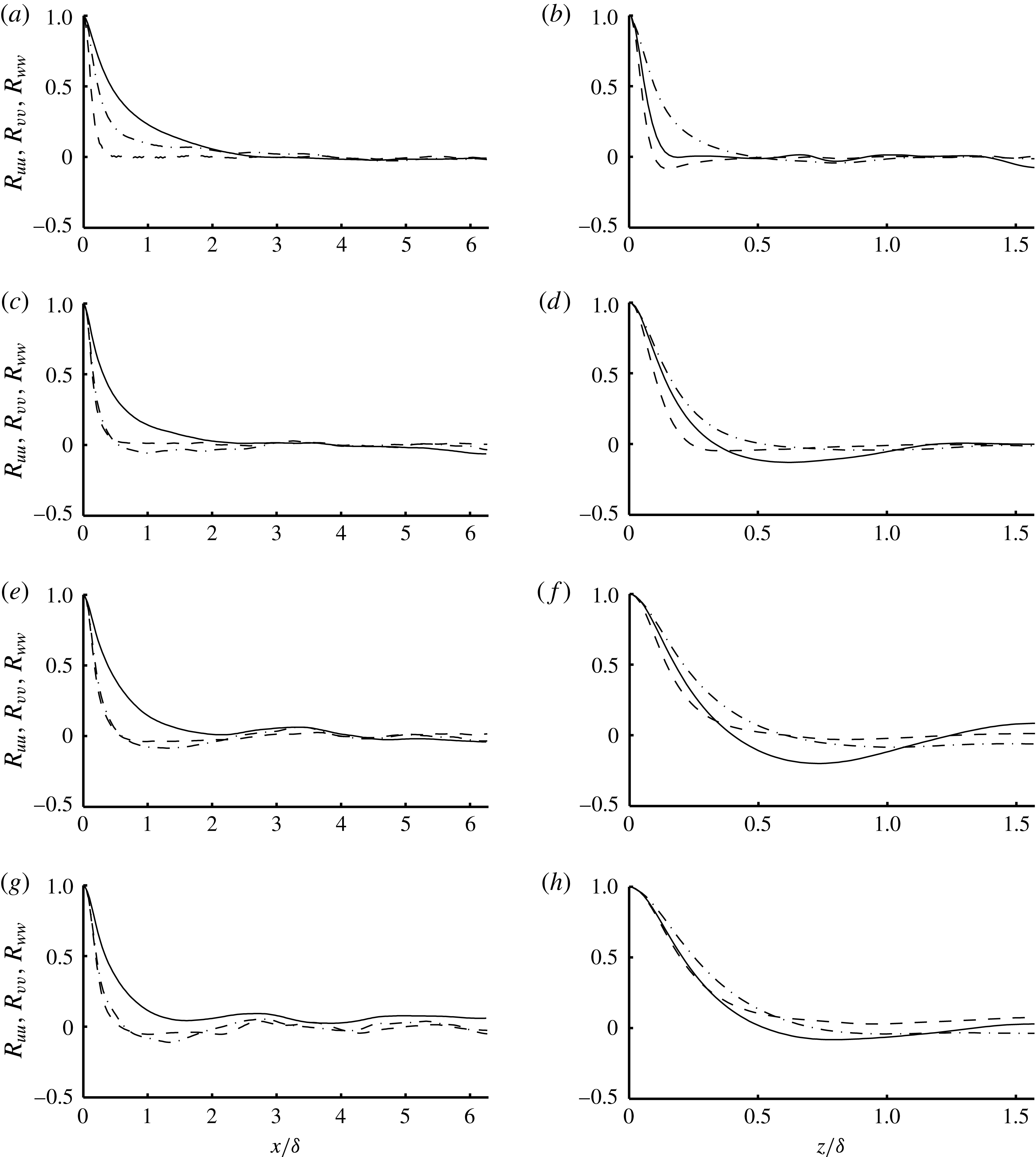
We have also performed a domain-size convergence study to ensure that the presented statistics are not affected by the computational domain size. To guide the selection of domain sizes for this study, we have analysed correlation statistics in both streamwise and spanwise directions at various distances from the wall. Details of this study are presented in the Appendix.
4. Results and discussion
4.1. Effects of geometry on pressure characteristics
First we compare the surface geometries of posts and streamwise ridges, focusing on their difference in pressure characteristics with fixed
 $L^{+}$
. With equal
 $W/L$
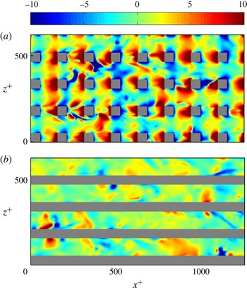
, both surfaces have similar mean and r.m.s. velocities, as shown in figure 5. While their turbulence intensities have no notable difference, the pressure fluctuations for posts are considerably higher. This contrast can be well explained by the detailed pressure contours at
 $y^{+}=0$
, shown for a particular instant in figure 6.
Comparison of statistics for
 $L^{+}\approx 155$
at
 $Re_{{\it\tau}}\approx 200$
. (a) Mean streamwise velocity profile; (b) velocity r.m.s. fluctuations; (c) pressure r.m.s. fluctuations.


Comparison of instantaneous pressure contours,
 $p^{+}=p/({\it\rho}u_{{\it\tau}}^{2})$
, at
 $y^{+}=0$
, for cases with
 $Re_{{\it\tau}}\approx 200$
and
 $L^{+}\approx 155$
. From blue to red, the fluctuations range between
 $-10$
and 10 wall units. (a) P155, (b) R155.

Schematic representation of stagnation phenomenon in (a) the streamwise/wall-normal plane and (b) the wall-parallel plane at
 $y^{+}=0$
.

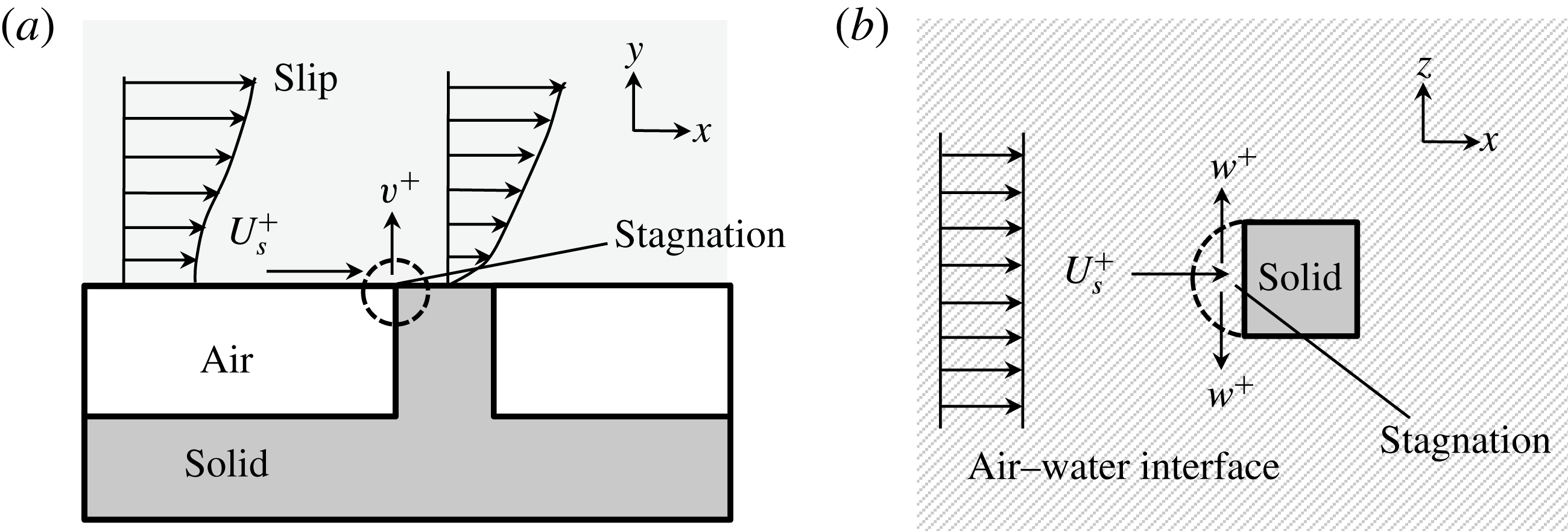
As schematically shown in figure 7, the slipping flow is diverted by the posts when it travels downstream, and a stagnation region with high pressure is formed immediately upstream of every post. This comparison is rather qualitative in the large texture size limit,
 $L^{+}\approx 155$
, but we will show later that the stagnation pressure is mainly a function of
 $L^{+}$
– through its dependence on
 $U_{s}^{+}$
, whereas the pressure fluctuations for streamwise ridges are less sensitive to the changes in slip or texture size.
4.2. Reynolds-number effect
Before discussing the effect of
 $L^{+}$
, it is worth briefly discussing the effect of a given texture with fixed
 $L^{+}$
at different
 $Re_{{\it\tau}}$
. According to the classical theory of wall turbulence, surface manipulations act only on the innermost region of the turbulent flow. From the point of view of the outer flow and its bulk properties, they only modify the intercept of the logarithmic velocity profile (Clauser Reference Clauser1956), in turn shifting the free-stream velocity and changing the friction coefficient. For the above statement to hold, however, the perturbations induced by the surface should only penetrate a small portion of the boundary layer (Jiménez Reference Jiménez2004). The depth of the penetration can be expected to scale with the typical length of the surface manipulations, in our case
 $L^{+}$
. A condition for the surface not to perturb the whole flow thickness would then be
 $L^{+}\ll Re_{{\it\tau}}$
. This condition was analysed for riblets, another drag-reducing surface, in García-Mayoral & Jiménez (Reference García-Mayoral and Jiménez2012), finding that in that case
 $L^{+}\approx 0.2Re_{{\it\tau}}$
was a sufficient condition. For our superhydrophobic posts at
 $Re_{{\it\tau}}\approx 200$
, that condition would clearly not be met by the cases of larger
 $L^{+}$
. Therefore, we have simulated the most critical case
 $L^{+}\approx 155$
also at
 $Re_{{\it\tau}}\approx 400$
. The results, of which some statistics are portrayed in figure 8, show that the influence of the texture extends only up to
 $y^{+}\approx 50{-}80$
. In the core of the channel, the flow behaves like that over smooth walls, albeit with a shifted velocity profile. Near the wall, the effect of the texture is essentially independent of the Reynolds number.
Comparison of statistics for post geometries with
 $L^{+}\approx 155$
at
 $Re_{{\it\tau}}\approx 200$
and
 $Re_{{\it\tau}}\approx 400$
. (a) Mean streamwise velocity profile; (b) velocity r.m.s. fluctuations; (c) pressure r.m.s. fluctuations. The intercept
 $B$
of the logarithmic region in the
 $U^{+}$
profile has been subtracted in (a) for better comparison of the outer region.

 $Re_{{\it\tau}}\approx 200$
, posts; ——,
 $Re_{{\it\tau}}\approx 200$
, smooth walls;

 $Re_{{\it\tau}}\approx 400$
, posts; - - - -,
 $Re_{{\it\tau}}\approx 400$
, smooth walls.

These results provide confidence in the relevance of our investigation to practical flows in which Reynolds number is higher. In other words, flow modifications by superhydrophobic surfaces are confined to the near-wall region, and are primarily controlled by
 $L^{+}$
and
 $\mathit{We}^{+}$
.
Note that the pressure fluctuations at the wall for smooth channels increase logarithmically with
 $Re_{{\it\tau}}$
, yet they do not reach values larger than
 $p_{\mathit{rms}}^{\prime +}\approx 3$
even at
 $Re_{{\it\tau}}\approx 4000$
(Hoyas & Jiménez Reference Hoyas and Jiménez2006; Lozano-Durán & Jiménez Reference Lozano-Durán and Jiménez2014). These are much smaller than the stagnation pressures reported here.
4.3. Turbulence statistics
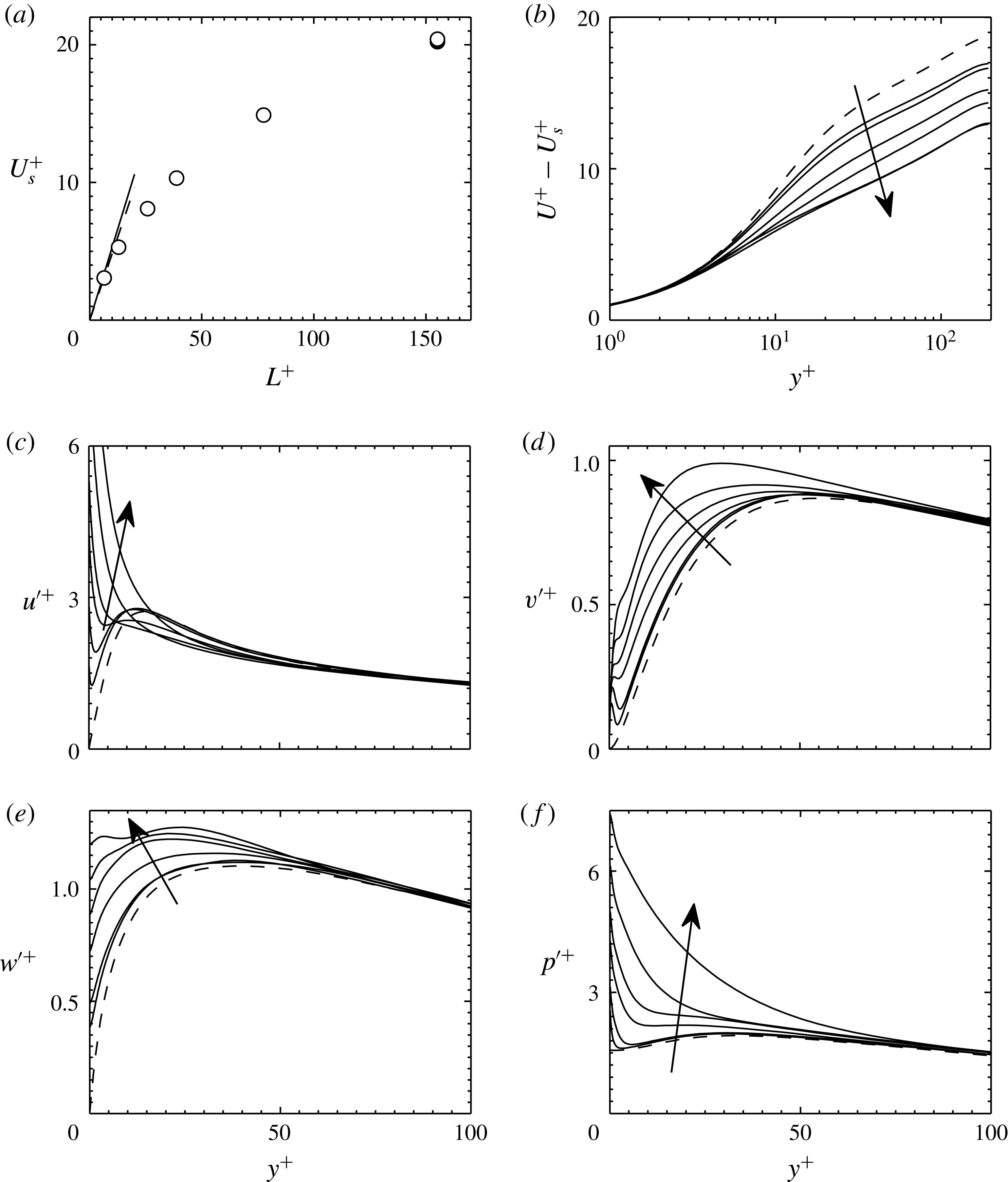
The slip velocity, mean velocity profile, turbulent intensities and pressure fluctuations for
 $L^{+}\approx 6{-}155$
are summarized in figure 9. Up to
 $L^{+}\approx 10$
, the effect of
 $L^{+}$
on the slip velocity follows a linear relationship, as shown in figure 9(a), and as predicted by the semi-analytical formula of Ybert et al. (Reference Ybert, Barentin and Cottin-Bizonne2007) and by our laminar flow simulation with the same texture layout,
 $$\begin{eqnarray}U_{s}^{+}=C_{Y}L^{+},\end{eqnarray}$$
where
 $C_{Y}=0.535$
for a solid fraction
 ${\it\phi}=1/9$
.
 $U_{s}$
can also be expressed in terms of a slip length,
 $b$
, so that in wall-unit scaling
 $U_{s}^{+}=b^{+}$
. The linear relationship of (4.1) breaks when the surface wavelength becomes
 $L^{+}\gtrsim 10$
. Deviation from linear slip theory is expected since the theory is based on Stokes’ flow equations, which lose their accuracy as the Reynolds number based on texture size becomes large. Our results show for the first time
 $U_{s}^{+}$
versus
 $L^{+}$
covering the entire range from the linear regime to the fully nonlinear large
 $L^{+}$
limit, for a three-dimensional superhydrophobic texture. Previous results have shown similar behaviour for two-dimensional streamwise ridges, covering
 $L^{+}$
values down to those of Park et al. (Reference Park, Park and Kim2013) and Türk et al. (Reference Türk, Daschiel, Stroh, Hasegawa and Frohnapfel2014).
Comparison of superhydrophobic posts for different
 $L^{+}$
at fixed
 $\mathit{Re}_{{\it\tau}}\approx 200$
, with arrows indicating increasing
 $L^{+}$
. (a) Slip velocity. The solid line indicates the theoretical prediction of Ybert et al. (Reference Ybert, Barentin and Cottin-Bizonne2007), the dashed line is the prediction from a laminar simulation with the same texture layout. The result for
 $L^{+}\approx 155$
and
 $\mathit{Re}_{{\it\tau}}\approx 400$
is included for reference with a solid symbol. (b) Mean velocity profile with the slip subtracted. (c–e) Streamwise, wall-normal and spanwise velocity r.m.s. fluctuations. (f) Pressure r.m.s. fluctuation. - - - -, smooth channel; ——, superhydrophobic posts.

Given that the large values of
 $U_{s}^{+}$
in our simulations can become comparable with the bulk and centreline velocities, they can obscure some of the effects of the surface on the velocity profile. For this reason, figure 9(b) compares the profiles offset by their respective slips,
 $U^{+}-U_{s}^{+}$
. The profiles show a behaviour similar to that of conventional roughness, for which the logarithmic region is increasingly extended towards the wall as the roughness size, or
 $L^{+}$
in our case, increases. The logarithmic region of the profile is given by
 $$\begin{eqnarray}U^{+}-U_{s}^{+}=\frac{1}{{\it\kappa}}\log (y^{+})+B,\end{eqnarray}$$
where
 ${\it\kappa}$
is Kármán constant and
 $B$
is the intercept of the logarithmic profile. As
 $L^{+}$
increases,
 $B$
decreases from its smooth-wall value
 $B\approx 5$
, and seems to reach asymptotically
 $B\approx 0$
for
 $L^{+}\gtrapprox 70$
. The decrease in
 $B$
through surface manipulations implies an increase in friction, which has been discussed and quantified thoroughly in the literature (Jiménez Reference Jiménez1994; Luchini Reference Luchini and Desideri1996; Spalart & McLean Reference Spalart and McLean2011; García-Mayoral & Jiménez Reference García-Mayoral and Jiménez2011a
). In the case of superhydrophobic surfaces, this deleterious effect is largely offset by the drag-reducing increase in
 $U_{s}^{+}$
. More interestingly, we note that for textures large enough,
 $L^{+}\gtrsim 70$
, the typical velocity profile in the viscous and buffer layers is completely destroyed, except for two wall units above the surface, and that the logarithmic profile seems to extend to the immediate vicinity of the wall. This suggests that, even if the surface remains flat, the distortion introduced by the alternating slip/no-slip conditions can completely disrupt the near-wall cycle, as conventional rough surfaces do (Jiménez Reference Jiménez2004).
Figure 9 also shows how the fluctuations intensify as
 $L^{+}$
increases. Those induced by the texture grow with the pattern wavelength, and the impact is most significant on the streamwise and pressure statistics. The large values of
 $u^{\prime }$
are essentially due to the large variations of
 $u$
between regions over the free-slip interface, where
 $u^{+}\approx 20$
, and the regions over the no-slip obstacles, where
 $u^{+}\approx 0$
. As the distribution of
 $u$
depends essentially on the
 $x{-}z$
position, the values fluctuate rather in space than in time. The wall-normal and spanwise velocity fluctuations do not experience such large surface effects, even though finite perturbations are still observable near the surface. A homogeneous slip length model (Min & Kim Reference Min and Kim2004; Busse & Sandham Reference Busse and Sandham2012) is not able to capture this trend, since it homogenizes the spatial variation of the velocity at the boundary.
The pressure fluctuations deserve special attention since they can be responsible for the breakup of the interface, and are analysed independently in § 4.5. The r.m.s. values exhibit dramatic increases near the wall, as
 $L^{+}$
increases, similar to those of
 $u^{\prime }$
. Note that this would not be the case for perfectly aligned ridges, such as those shown in figure 5(c).
In all of the profiles investigated, the effect of the texture layout decays rapidly with
 $y^{+}$
, and even for the larger
 $L^{+}\approx 150$
it does not extend beyond
 $y^{+}\approx 60$
. This extension of the distortion of the fluctuations across the full buffer layer is likely connected to the disruption of the near-wall cycle mentioned above. For textures of realistic size, though, and up to
 $L^{+}\approx 15$
, their presence only affects the r.m.s. values in small near-wall kinks confined within the viscous sublayer,
 $y^{+}\lesssim 5$
.
4.4. Decomposition of fluctuations
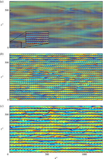
To better understand the statistical data, instantaneous distributions of the wall-normal vorticity and the pressure on the superhydrophobic surface are portrayed in figures 10 and 11 (supplementary movies are available online at http://dx.doi.org/10.1017/jfm.2015.573). At small
 $L^{+}$
, the distribution of
 ${\it\omega}_{y}^{+}$
is dominated by the footprint of near-wall turbulent streaks, with the exception of the small-scale shedding of flow from the posts. This shedding, however, becomes increasingly important as
 $L^{+}$
increases, and becomes dominant for
 $L^{+}\gtrsim 35$
.
Comparison of instantaneous wall-normal vorticity,
 ${\it\omega}_{y}^{+}$
, contours at
 $y=0$
, for cases (a) P13, (b) P26 and (c) P39. From blue to red, the fluctuations range between
 $-1.2$
and 1.2 wall units. The rectangular inset in (a) is a magnification of the boxed region in the main plot.

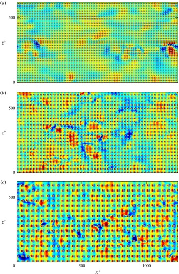
Comparison of instantaneous pressure contours,
 $p^{+}$
, at
 $y=0$
, for cases (a) P13, (b) P26 and (c) P39. From blue to red, the fluctuations range between
 $-10$
and 10 wall units.

Two distinct contributions can also be observed in the instantaneous pressure fluctuations near the wall as shown in figure 11. The first is the footprint of turbulent pressure fluctuations as they are advected downstream, with typical length scales
 ${\sim}100{\it\nu}/u_{{\it\tau}}$
, and similar to those observed over smooth walls. The second is a stationary distribution caused by the stagnation of flow in front of and behind the posts. Again, the former dominates for small textures, and the latter for large ones.
To analyse separately the contribution due to the overlying turbulence and that due to the surface texturing, for any variable
 $q$
we decompose its fluctuations
 $q^{\prime }$
into a spatially coherent component
 $\tilde{q}$
, which is time-independent, and a random component
 $q^{\prime \prime }$
, so that
 $$\begin{eqnarray}q(x,z,y,t)=\bar{q}(y)+q^{\prime }(x,z,y,t)=\bar{q}(y)+\tilde{q}(\tilde{x},\tilde{z},y)+q^{\prime \prime }(x,z,y,t),\end{eqnarray}$$
where
 $\tilde{x}=\text{modulo}(x,L_{x})$
and
 $\tilde{z}=\text{modulo}(z,L_{z})$
are the relative streamwise and spanwise coordinates within each pattern periodic unit, and where the coherent component
 $\tilde{q}$
is averaged over time and over the number of periodic units. This type of decomposition, into ‘coherent’ and ‘random’ components, was introduced by Reynolds & Hussain (Reference Reynolds and Hussain1972), and has been extensively used to analyse turbulent flows over complex surfaces (Choi, Moin & Kim Reference Choi, Moin and Kim1993; Jiménez et al.
Reference Jiménez, Uhlman, Pinelli and Kawahara2001; García-Mayoral & Jiménez Reference García-Mayoral and Jiménez2011b
; Jelly et al.
Reference Jelly, Jung and Zaki2014; Türk et al.
Reference Türk, Daschiel, Stroh, Hasegawa and Frohnapfel2014).
Decomposition of fluctuation statistics for different
 $L^{+}$
at fixed
 $\mathit{Re}_{{\it\tau}}\approx 200$
, with arrows indicating increasing
 $L^{+}$
. (a)
 $\tilde{u} _{\mathit{rms}}^{+}$
, (b)
 $u_{\mathit{rms}}^{\prime \prime +}$
, (c)
 $\tilde{v}_{\mathit{rms}}^{+}$
, (d)
 $v_{\mathit{rms}}^{\prime \prime +}$
, (e)
 $\tilde{w}_{\mathit{rms}}^{+}$
, (f)
 $w_{\mathit{rms}}^{\prime \prime +}$
, (g)
 $\tilde{p}_{\mathit{rms}}^{+}$
, (h)
 $p_{\mathit{rms}}^{\prime \prime +}$
. - - - -, smooth channel; ——, superhydrophobic posts;
 $\cdots \cdots$
, superhydrophobic posts,
 $\mathit{Re}_{{\it\tau}}\approx 400$
,
 $L^{+}\approx 155$
.

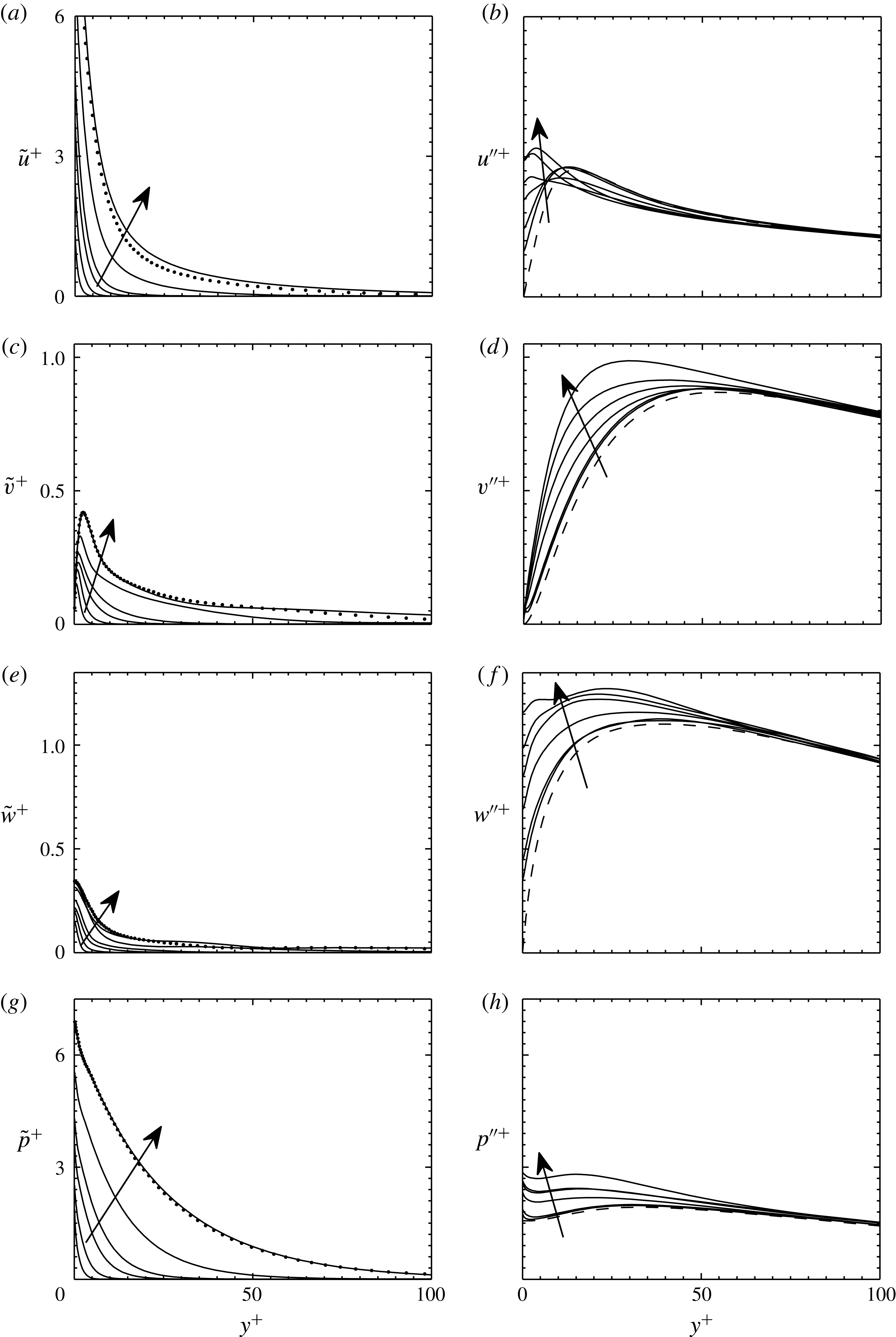
The result of applying this decomposition to the velocity and pressure fluctuations is illustrated in figure 12. The figure shows for instance that most of the previously observed change in
 $u^{\prime }$
when computing the raw r.m.s. is due to the coherent distribution
 $\tilde{u}$
, while the turbulent component
 $u^{\prime \prime }$
remains essentially unaltered at magnitudes similar to those in a smooth-wall case. In all quantities plotted, the turbulent component of the fluctuations is augmented with increasing texture size, but the augmentation is rather modest and confined to the near wall (
 $y^{+}\lessapprox 60$
).
As discussed in § 4.2, the effect of the surface is essentially independent of Reynolds number, and the coherent contribution remains roughly constant as shown in figure 12 for
 $Re_{{\it\tau}}\approx 200$
and
 $Re_{{\it\tau}}\approx 400$
.
As
 $L^{+}$
increases, the coherent component of the pressure increases dramatically, while the random contribution remains close to that of smooth channels. This dramatic increase of
 $\tilde{p}^{+}$
with
 $L^{+}$
sets a limit to the pattern size for practical applications, since the high stagnation pressures are bound to deform and eventually break up the entrapped air bubbles.
4.5. Scaling and self-similarity of stagnation pressure
In the limit of vanishing spacing,
 $L^{+}\rightarrow 0$
, the flow in the vicinity of the texture is dominated by viscous effects and can be analysed as a Stokes flow (Luchini, Manzo & Pozzi Reference Luchini, Manzo and Pozzi1991). In that regime, dimensional analysis predicts that
 $\tilde{p}^{+}\sim 1$
is independent of
 $U_{s}^{+}$
. Conversely, for
 $L^{+}\rightarrow \infty$
, inertial effects are dominant and dimensional analysis predicts
 $\tilde{p}\sim {U_{s}^{+}}^{2}$
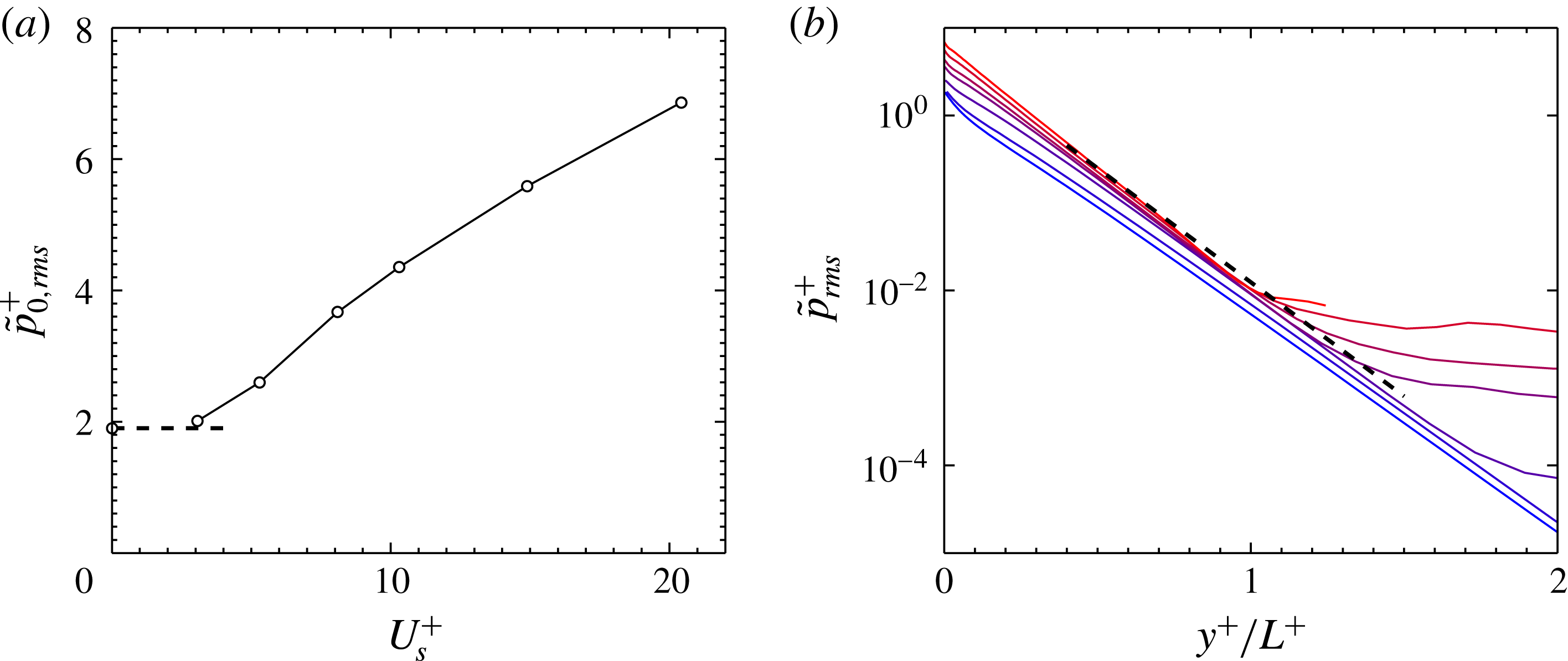
. To check the actual scaling observed in our DNS, we first focus on the values of
 $\tilde{p}^{+}$
at
 $y^{+}=0$
,
 $\tilde{p}_{0}^{+}$
, shown in figure 13(a). The value for
 $L^{+}\approx 6$
is very close to that predicted for
 $L^{+}\rightarrow 0$
from a viscous, laminar simulation. However, from there on
 $\tilde{p}_{0}^{+}$
seems to exhibit a linear scaling with
 $U_{s}^{+}$
, which is close to
 $$\begin{eqnarray}\tilde{p}_{0,\mathit{rms}}^{+}=0.28U_{s}^{+}+1.26.\end{eqnarray}$$
This behaviour is intermediate to those predicted for
 $L^{+}\rightarrow 0$
and
 $L^{+}\rightarrow \infty$
.
(a) Coherent pressure fluctuation values at
 $y^{+}=0$
, with the dashed line marking the asymptotic limit for a laminar solution at
 $L^{+}\rightarrow 0$
. (b) Self-similar behaviour of the r.m.s. of the stagnation contribution to the pressure,
 $\tilde{p}(y)$
. From blue to red, increasing
 $L^{+}$
from
 $L^{+}\rightarrow 0$
to
 $L^{+}\approx 155$
. The dashed line indicates
 $\tilde{p}^{+}\sim \exp (-6y^{+}/L^{+})$
.

The coherent pressure
 $\tilde{p}^{+}$
also exhibits a self-similar behaviour when its variation with
 $y^{+}$
is considered. Figure 13(b) shows that
 $\tilde{p}_{\mathit{rms}}^{+}(y^{+},L^{+})$
satisfies a self-similar scaling that can be expressed as
 $$\begin{eqnarray}\tilde{p}_{\mathit{rms}}^{+}\sim \exp \left(-\frac{2{\rm\pi}}{L^{+}}y^{+}\right).\end{eqnarray}$$
The exponential decay in
 $y^{+}$
is reminiscent of a solution to the Laplace equation with periodic behaviour in the wall-tangential direction with period
 $L^{+}$
. Such a solution is consistent with solutions over patterned surfaces in the Stokes flow limit (Belyaev & Vinogradova Reference Belyaev and Vinogradova2010; Kamrin, Bazant & Stone Reference Kamrin, Bazant and Stone2010). However, it is remarkable that the same scaling still holds in the turbulent flow regimes for
 $L^{+}$
values as high as about a hundred.
Self-similarity is not only observed in the r.m.s. value of
 $\tilde{p}$
, but also in its
 $\tilde{x}{-}\tilde{z}$
spatial distribution, as shown in figure 14(a) for
 $\tilde{p}_{0}^{+}$
.
(a) Streamwise distribution of
 $\tilde{p}$
at
 $y^{+}=0$
for the
 $\tilde{x}$
-line running through the middle of the posts. Each case has been scaled with its in-plane r.m.s. value. From blue to red,
 $L^{+}$
increases from
 $L^{+}\approx 6$
to
 $L^{+}\approx 155$
. The black dashed lines correspond to the laminar solution for
 $L^{+}\rightarrow 0$
. The black solid lines mark the location of the post. The points are interpolated with a spline. (b) Interface deformation,
 ${\it\eta}^{+}$
, at
 $L^{+}\approx 155$
,
 $Re_{{\it\tau}}\approx 200$
and
 $\mathit{We}^{+}=10^{-3}$
. From blue to red, the lines are plotted in evenly spaced spanwise locations, and the red ones are on the plane where the posts are located.

 ${\rm\Delta}x^{+}\approx 6.4$
,
 ${\rm\Delta}z^{+}\approx 3.2$
;

 ${\rm\Delta}x^{+}\approx 3.2$
,
 ${\rm\Delta}z^{+}\approx 1.6$
;

 ${\rm\Delta}x^{+}\approx 2.2$
,
 ${\rm\Delta}z^{+}\approx 1.1$
.

4.6. Interface deformation
The analysis of the pressure is interesting in itself, but for practical applications it is even more interesting to analyse how that pressure would deform the interface. An additional advantage is that, while the pressure fields are singular at the solid/interface edges, the deformation fields are not, and they are therefore less sensitive to the grid resolution. Interface deformation can be obtained from the stagnation pressure using (2.3). The contact angle is defined at trailing and leading edges of the posts as
 $$\begin{eqnarray}\displaystyle & \displaystyle {\it\theta}_{L}=\frac{{\rm\pi}}{2}+\text{tan}^{-1}\left(\left.\frac{\text{d}{\it\eta}}{\text{d}x}\right|_{L}\right), & \displaystyle\end{eqnarray}$$
 $$\begin{eqnarray}\displaystyle & \displaystyle {\it\theta}_{T}={\rm\pi}-\text{tan}^{-1}\left(\left.\frac{\text{d}{\it\eta}}{\text{d}x}\right|_{T}\right), & \displaystyle\end{eqnarray}$$
 $\text{d}{\it\eta}/\text{d}x$
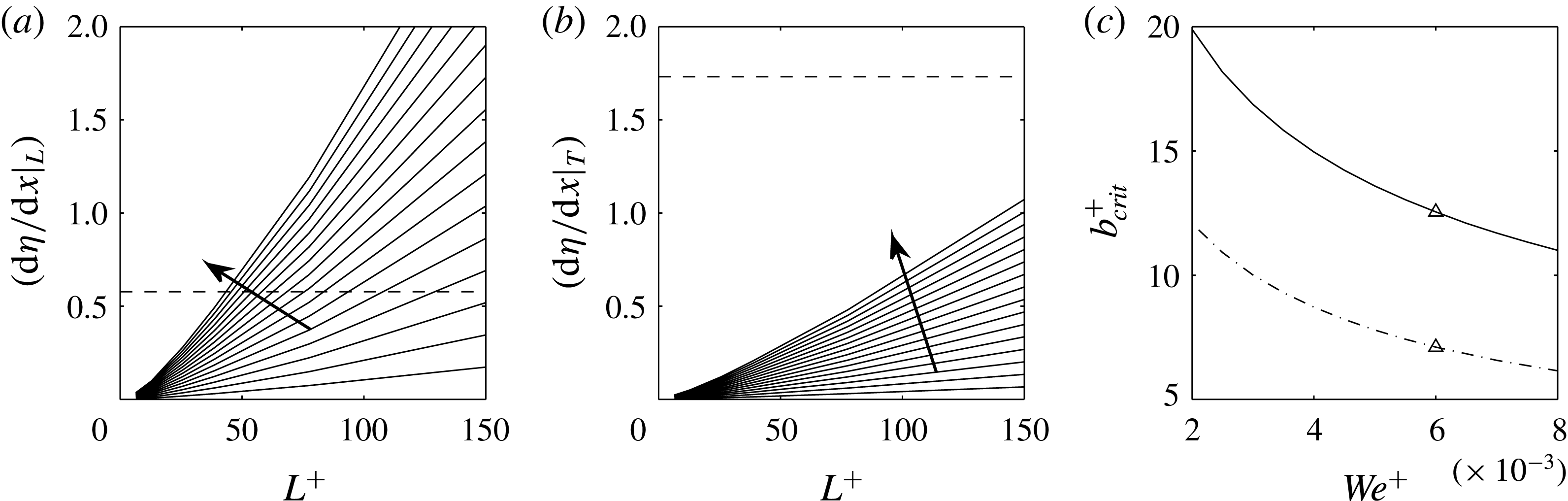
, is measured from the spline interpolation at the contact point. The interface is deflected down in stagnation pressure regions, and the maximum interface slope occurs at the midpoint of the posts’ leading edge, as shown in figure 14(b). One possible failure scenario is related to this maximum deformation, with its onset determined by
 ${\it\theta}_{L}$
becoming equal to the microscopic advancing contact angle,
 ${\it\theta}_{adv}$
. At this onset the air–water interface will not remain pinned at the edge of the post and will start moving down till further wetting the post. We consider this condition to be the onset of failure of the superhydrophobic surface. A similar failure mechanism would pertain when
 ${\it\theta}_{T}$
becomes equal to the microscopic receding contact angle,
 ${\it\theta}_{rec}$
.
This procedure allows us to establish a criterion to estimate a critical
 $L^{+}$
for stable drag reduction as a function of
 $\mathit{We}^{+}$
. We note that the linear Young–Laplace equation, as shown in (2.3), is only valid for small deformations, where
 $\text{d}{\it\eta}/\text{d}x\ll 1$
. However, to obtain only a rough estimate of the onset of interface breakage, we resort here to linear solutions. Additionally we assume a representative microscopic advancing contact angle
 ${\it\theta}_{adv}=120^{\circ }$
(equivalent to
 $\text{d}{\it\eta}/\text{d}x=0.58$
), consistent with the best hydrophobic materials. Note that the apparent macroscopic contact angle, which is typically closer to 180° for a textured material, is not the relevant parameter in this subtexture analysis.
Interface slope at the post edge as a function of
 $L^{+}$
, for different
 $\mathit{We}^{+}$
ranging from
 $5\times 10^{-4}$
to
 $8\times 10^{-3}$
with successive intervals of
 $5\times 10^{-4}$
at (a) the leading and edge (b) the trailing edge. Arrows indicate increasing
 $\mathit{We}^{+}$
. The black dashed line represents
 ${\it\theta}_{L}=120^{\circ }$
in (a) and
 ${\it\theta}_{T}=120^{\circ }$
in (b). The intersection of the dashed line with a solid line represents the critical
 $L^{+}$
for the corresponding
 $\mathit{We}^{+}$
. For each critical point, the resulting slip length is plotted as a function of
 $\mathit{We}^{+}$
in (c). The dashed-dot line represents the same calculation for a material with a critical contact angle of 100°. The triangle symbol indicates a typical
 $\mathit{We}^{+}$
corresponding to
 $U_{\infty }=10~\text{m}~\text{s}^{-1}$
.

Figure 15(a) shows the computed interface slope at the pinned location as a function of
 $L^{+}$
for different values of
 $\mathit{We}^{+}$
. For each
 $\mathit{We}^{+}$
, as one increases the
 $L^{+}$
(e.g. experimentally by increasing the texture size, for fixed channel height, pressure gradient and fluid properties) the critical slope will be reached at some critical value of texture size,
 $L_{crit}^{+}$
. Figure 15(b) shows the same for the slope at the trailing edge of the post, indicating that the leading edge slope is more critical to failure. Figure 15(c) summarizes these results by showing the critical values as a function of
 $\mathit{We}^{+}$
. Here, we have used values of
 $U_{s}^{+}$
from figure 9(a) and have directly reported the bounds on achievable slip length.
As
 $\mathit{We}^{+}$
increases,
 $L_{crit}^{+}$
, and thus the achievable slip length, decreases, suggesting an upper bound for practical applications. Proper non-dimensionalization of the Young–Laplace equation together with (4.4) suggests the following scaling relation for the onset of interface breakage:
 $$\begin{eqnarray}\displaystyle \mathit{We}^{+}U_{s}^{+}L^{+}=O(1), & & \displaystyle\end{eqnarray}$$
where the constant of order one on the right-hand side depends on the advancing contact angle. Remarkably, the same relation would hold in the limit of a nonlinear Young–Laplace equation for large deformations; only the constant on the right-hand side would be different.
The results shown in figure 15(c) have significance in practical applications and in the design of superhydrophobic surfaces. We note that the defined
 $\mathit{We}^{+}={\it\rho}u_{{\it\tau}}{\it\nu}/{\it\sigma}$
is mostly controlled by the free-stream velocity and only has logarithmic dependence on the boundary layer thickness in turbulent flows (Lozano-Durán & Jiménez Reference Lozano-Durán and Jiménez2014). For practical purposes
 $u_{{\it\tau}}$
can be estimated to be 20–30 times smaller than the free-stream velocity. For example, for a free-stream velocity of
 $10~\text{m s}^{-1}$
,
 $\mathit{We}^{+}$
is in the range
 $(5{-}7)\times 10^{-3}$
for typical boundary layers. Assuming the midpoint value of
 $\mathit{We}^{+}=6\times 10^{-3}$
, figure 15(a) predicts
 $L_{crit}^{+}\sim 50$
, which is dimensionally of the order of
 $L=50{\it\nu}/u_{{\it\tau}}\sim 100~{\rm\mu}\text{m}$
. Figure 15(c) predicts that for this
 $\mathit{We}^{+}$
the maximum achievable slip velocity is about 12 in plus units.
We note that the developed model predicts an upper bound for robustness of superhydrophobic surfaces, by considering only one failure mechanism. Other failure modes such as hydrostatic pressure (if not treated) and gas dissolutions (if exposed to water for a long time) should be considered in addition to what was presented here.
Lastly, we note that the presented model uses only a one-way coupled system, and ignores the effects of interface deformation back on the flow field. A more accurate analysis should include interface dynamics fully coupled with the flow. Preliminary investigations indicate that pressure fluctuations in a fully coupled system are slightly higher than those in the one-way coupled systems considered here (Seo, García-Mayoral & Mani Reference Seo, García-Mayoral and Mani2014), therefore reaffirming the fact that the developed model predicts only an upper bound for stable operation of the superhydrophobic surface.
5. Summary and discussion
The work presented here has investigated the dynamics of turbulent flows over superhydrophobic textured walls with entrapped gas pockets. We presented for the first time simulations for a wide range of scales for a three-dimensional texture geometry: from small textures of the order of
 $L^{+}=6$
to very large textures with
 $L^{+}=155$
. We showed that the small-texture limit results in a slip velocity as predicted by the linear theory of Ybert et al. (Reference Ybert, Barentin and Cottin-Bizonne2007), and found the threshold of validity of linear theory to be around
 $L^{+}\sim 10$
.
We presented three dimensionless parameters that describe the system. These are the boundary layer Reynolds number,
 $Re_{{\it\tau}}$
, the texture dimension in viscous units,
 $L^{+}$
, and the Weber number in viscous units,
 $\mathit{We}^{+}={\it\rho}u_{{\it\tau}}{\it\nu}/{\it\sigma}$
. The defined Weber number is convenient since it is dominantly controlled by the free-stream velocity, and allows easier communication of our results in terms of dimensional parameters. Furthermore, it does not assume any a priori scaling of pressure with
 $L^{+}$
, and with these parameters all texture-dependent effects are controlled through a single dimensionless parameter,
 $L^{+}$
.
By investigating different Reynolds numbers, we showed that the deviation in flow statistics due to texture is independent of Reynolds number when plotted in terms of inner dimensions. Furthermore, texture effects penetrate up to
 $y^{+}$
of order
 ${\sim}60$
, and beyond this point the profiles are very similar to smooth-wall turbulent boundary layers. These findings helped to establish the relevance of our calculations to flows of higher Reynolds number.
We investigated pressure fluctuations in terms of two modes: an unsteady turbulent mode and a steady coherent mode solely controlled by the texture geometry. While the pressure magnitude of the turbulent mode is of the same order as that in a smooth-wall turbulent boundary layer, the pressure field associated with the texture geometry was shown to increase significantly with the texture size. Particularly for a three-dimensional post geometry, this pressure increase was more significant (in comparison to two-dimensional streamwise ridges) due to the stagnation of slip velocity with the edge of the posts. We showed that the coherent pressure field has a self-similar behaviour for a wide range of
 $L^{+}$
, and that it scales linearly with the slip velocity. Lastly, we analysed the interface deformation due to the resulting pressure fields and predicted threshold conditions for interface failure and transition to the Wenzel state. Combining the knowledge of pressure fluctuations and interface deformation, it becomes clear that the implementation of large textures can deteriorate the stability of the gas pockets. This is observed in various experiments (Aljallis et al.
Reference Aljallis, Sarshar, Datla, Sikka and Jone2013; Bidkar et al.
Reference Bidkar, Leblanc, Kulkarni, Bahadur, Ceccio and Perlin2014) but not predicted by the state-of-the-art simulations. The present results may discourage further focus on post layouts, and indeed most recent studies have focused on ridges (Daniello et al.
Reference Daniello, Waterhouse and Rothstein2009; Woolford et al.
Reference Woolford, Prince, Maynes and Webb2009; Park et al.
Reference Park, Sun and Kim2014). However, streamwise ridges can only be implemented in academic scenarios. In practice, the fabrication of perfectly aligned ridges is complicated and expensive. Moreover, ridge geometries can suffer the same stagnation issues when misaligned to the flow direction. On the other hand, in the small-wavelength limit of practical applications,
 $L^{+}\approx 5$
, the stagnation effect is small and posts become an attractive option. In this limit, slip velocities of order
 $U_{s}^{+}\simeq 3$
are still achievable, implying drag reductions of the order of 15 %. Post geometries are also more similar to realistic superhydrophobic surfaces involving more practical ways for mass production, such as the randomly distributed roughness spray coatings recently tested in Aljallis et al. (Reference Aljallis, Sarshar, Datla, Sikka and Jone2013), Bidkar et al. (Reference Bidkar, Leblanc, Kulkarni, Bahadur, Ceccio and Perlin2014) and Srinivasan et al. (Reference Srinivasan, Kleingartner, Gilbert, Cohen, Milne and McKinley2015). Their observations agree qualitatively with the deterioration of the stability of the gas pockets reported here.
Acknowledgement
This work was supported by the Office of Naval Research under grant 3002451214. The authors greatly appreciate the Kwanjeong Educational Foundation for the funding support for J.S.
Supplementary movies
Supplementary movies are available at http://dx.doi.org/10.1017/jfm.2015.573.
Appendix. Convergence of statistics with respect to the computational domain size
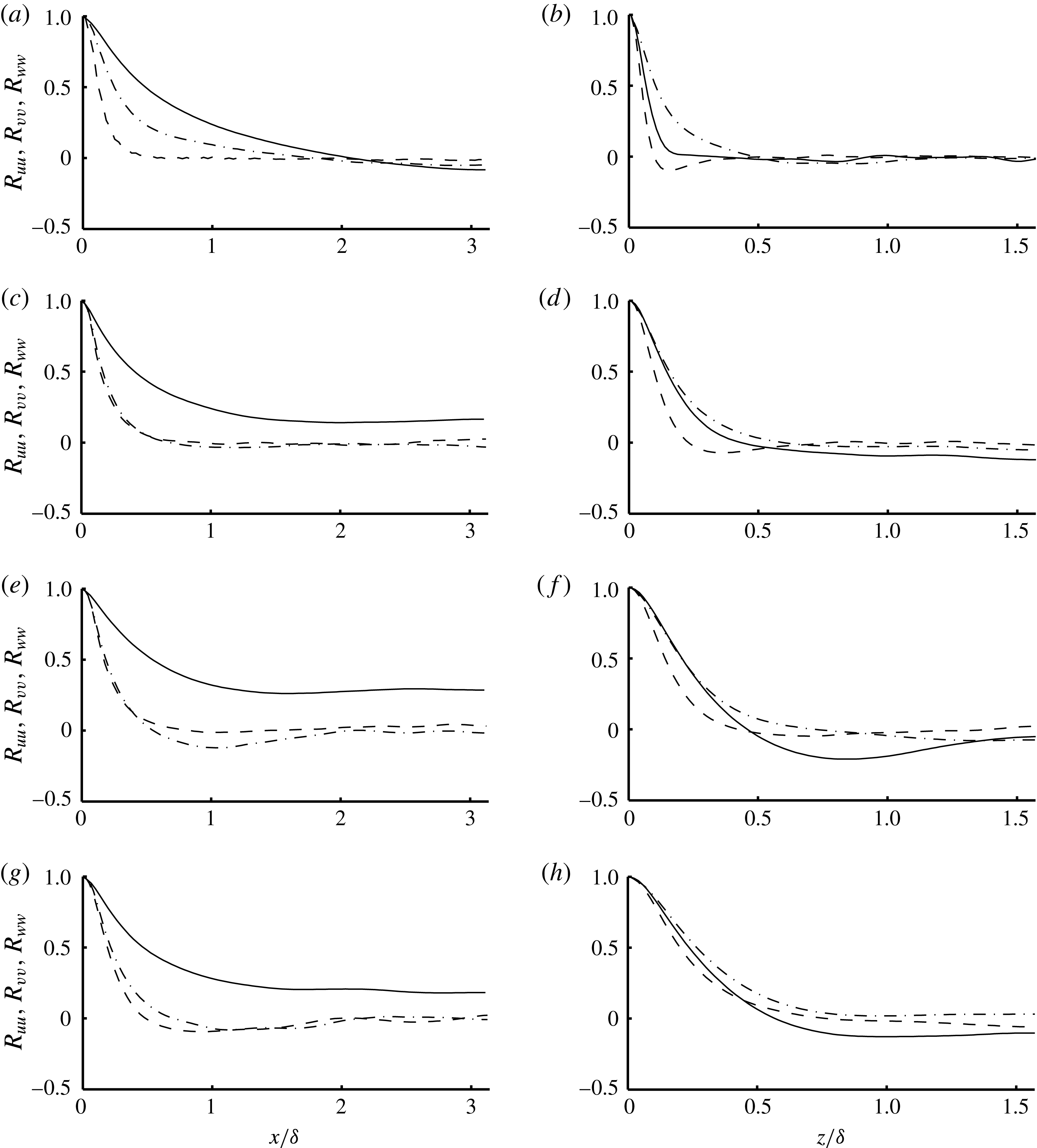
We present here briefly a comparison of DNS statistics obtained from simulations over different domain sizes. To guide the critical directions over which we should change the domain, we first performed an analysis of correlation statistics in both streamwise and spanwise directions for all three components of the velocity field. As shown in figure 16, with the exception of
 $R_{uu}$
as a function of streamwise separation distance, all other correlations show a satisfactory drop to zero. This indicates that a convergence study is needed in which the domain size is changed in the streamwise direction.
Two-point correlations along streamwise (a,c,e,g) and spanwise (b,d,f,h) directions for
 $L^{+}\approx 155$
,
 $D_{x}=2{\rm\pi}$
and
 $D_{z}={\rm\pi}$
. ——,
 $R_{uu}$
; - - - -,
 $R_{vv}$
; — ⋅ —,
 $R_{ww}$
. (a,b)
 $y^{+}=4.8552$
,
 $y/{\it\delta}=0.024583$
; (c,d)
 $y^{+}=50.3651$
,
 $y/{\it\delta}=0.25501$
; (e,f)
 $y^{+}=98.9805$
,
 $y/{\it\delta}=0.50117$
; (g,h)
 $y^{+}=197.5$
,
 $y/{\it\delta}=1$
.

Two-point correlations along streamwise (a,c,e,g) and spanwise (b,d,f,h) directions for
 $L^{+}\approx 155$
,
 $D_{x}=4{\rm\pi}$
and
 $D_{z}={\rm\pi}$
. ——,
 $R_{uu}$
; - - - -,
 $R_{vv}$
; — ⋅ —,
 $R_{ww}$
. (a,b)
 $y^{+}=4.8552$
,
 $y/{\it\delta}=0.024583$
; (c,d)
 $y^{+}=50.3651$
,
 $y/{\it\delta}=0.25501$
; (e,f)
 $y^{+}=98.9805$
,
 $y/{\it\delta}=0.50117$
; (g,h)
 $y^{+}=197.5$
,
 $y/{\it\delta}=1$
.

Comparison of statistics for
 $L^{+}\approx 155$
at
 $Re_{{\it\tau}}\approx 200$
. (a) Mean streamwise velocity profile; (b) velocity r.m.s. fluctuations; (c) pressure r.m.s. fluctuations.

 $D_{x}=2{\rm\pi},D_{z}={\rm\pi}$
;

 $D_{x}=4{\rm\pi},D_{z}={\rm\pi}$
.

We performed a new calculation for the presented case, in which the streamwise domain is doubled to
 $D_{x}=4{\rm\pi}$
. Figure 17 shows that for this case all correlations drop satisfactorily to zero. Figure 18 confirms that the velocity statistics are not affected by the change in the domain size. Specifically, the mean flow rate was within 0.25 % of the two calculations and the slip velocity was within 0.5 %.