2 The model

An $M/M/k/\ell +M$ queue is considered, that is, a queue with Poisson arrivals, exponential service time, exponential abandonment time, k servers and capacity $\ell $ so that no more than $\ell $ customers can be in the system at any time, with $\ell \geq k$ . A customer is blocked if they call when all lines are busy. It is also assumed that a caller cannot abandon once the service has commenced. Customers are served on a first-come, first-served basis in a work-conserving manner.

Let $\lambda $ be the arrival rate of customers, $\mu $ be the service rate and $\theta $ be the abandonment rate. The system is modelled as a continuous-time Markov chain [Reference Kleinrock14]. Let $Y(t)$ denote the total number of customers in the system at time t for $t> 0$ with state space ${S_y = \{0,1,\ldots ,\ell \}}$ .

From state j, transitions occur as follows. An arrival increases the state to $j+1$ at rate $\lambda $ when $j < \ell $ ; otherwise, arrivals are blocked. Departures occur either due to service completions or abandonment. If $j \leq k$ , there are j customers in service and $0$ customers in the queue. If $j> k$ , there are k customers in service and $j - k$ customers in the queue. Hence, the number of customers in service is $\min (j,k)$ and the number of customers in the queue is $\max (0,j-k)$ . This implies that the total rate from state j to $j-1$ is given by

$$ \begin{align*} \min(j,k)\mu + \max(0,j-k)\theta. \end{align*} $$

Thus, the transition rates are

$$ \begin{align*} q_{j,j+1} = \lambda \mathbb{1}_{\{j < \ell\}}, \quad q_{j,j-1} = \min(j,k)\mu + \max(0,j-k)\theta. \end{align*} $$

3 The waiting time distribution of a tagged caller

The aim of this paper is to compute the waiting time distribution of arriving customers. The analysis begins by studying the waiting time of a tagged caller whose position in the system is known upon arrival.

Specifically, the focus is on the time a caller spends waiting in the queue before being assigned to an available server. Thus, the waiting time ends when the caller enters service. Attention is restricted to cases where the waiting time is strictly positive, that is, when the tagged caller joins the queue. If an arriving customer finds fewer than k customers in the system, they enter service immediately and therefore experience zero waiting time.

To analyse the waiting time, a second continuous-time Markov chain $X(t)$ is introduced to represent the position of the tagged caller in the system at time t, conditional on the caller being in the queue. The state space of $X(t)$ , denoted by $S_x$ , is given by the waiting positions $\{k+1, k+2, \ldots , \ell \}$ . Since the position of the tagged caller can only decrease over time, $X(t)$ evolves as a pure death process.

The process $X(t)$ can be absorbed in two ways. The first occurs when the tagged caller enters service and then the absorption time is the waiting time of interest. The second occurs when the tagged caller abandons the queue, in which case the waiting time is taken to be infinite. Therefore, the waiting time is a defective random variable, as it can take the value $\infty $ with positive probability.

When $X(t) = i$ , there are $i-1$ customers ahead of the tagged caller, of whom k are in service and $i-1-k$ are waiting in the queue. Service completions occur at rate $k\mu $ , while customers ahead of the tagged caller abandon the queue at rate $(i-1-k)\theta $ . Hence, the total rate of transition from state i to $i-1$ is given by $k\mu + (i-1-k)\theta $ .

In addition, the tagged caller may abandon the queue at rate $\theta $ , in which case the process is absorbed. Therefore, the total transition rate out of state i is given by ${k\mu + (i-k)\theta }$ .

Let $\tau _i$ denote the sojourn time in state i. Then, $\tau _i$ is exponentially distributed with rate $k\mu + (i-k)\theta $ .

Let $W_i$ denote the waiting time of a tagged caller who arrives in position i. If the caller abandons the system before entering service, then $W_i = \infty $ . For $y> 0$ , let $\Xi _i(y)$ denote the waiting time distribution of $W_i$ , that is,

$$ \begin{align*} \Xi_i(y) = \mathbb{P}(W_i \le y). \end{align*} $$

Since $W_i$ is a defective random variable, the limit of $\Xi _i(y)$ as $y \to \infty $ is equal to the probability that the caller is eventually served. The Laplace–Stieltjes transform (LST) of $\Xi _i(y)$ , denoted by $\bar {\Xi }_i(s)$ , is given by

$$ \begin{align*} \bar{\Xi}_i(s) = \int_0^\infty e^{-s t}\, d\Xi_i(t) = \mathbb{E}(e^{-s W_i}). \end{align*} $$

The aim is to compute $\mathbb {E}(e^{-sW_i})$ . If $i \leq k$ , that is, the tagged caller immediately enters service upon arrival, $W_i = 0$ . Hence,

(3.1) $$ \begin{align} \mathbb{E}(e^{-s W_i}) = 1. \end{align} $$

To compute $\mathbb {E}(e^{-sW_i})$ when the tagged caller joins the queue, a first-step analysis is used. When the tagged caller is in position i, at the next event, there are two possibilities.

• • The tagged caller abandons with probability

  $$ \begin{align*} \frac{\theta}{(i-k)\theta + k\mu}, \end{align*} $$
  in which case $W_i = \infty $ and, hence, $e^{-sW_i} = 0$ .

• • The position of the tagged caller decreases to $i-1$ with probability

  $$ \begin{align*} \frac{(i-1-k)\theta + k\mu}{(i-k)\theta + k\mu}, \end{align*} $$
  due to either a service completion or abandonment of a customer ahead. In this case, $W_i = \tau _i + W_{i-1}.$

Conditioning on $\tau _i$ and the next event yield

$$ \begin{align*} \mathbb{E}(e^{-s W_i}) = \mathbb{E}( \mathbb{E}(e^{-s W_i} \mid \tau_i, X(\tau_i))). \end{align*} $$

Only the transition to $i-1$ contributes, since the abandonment case yields zero. Denote the probability density function of $\tau _i$ by

$$ \begin{align*} f_{\tau_i}(t) = \bigl((i-k)\theta + k\mu\bigr) e^{-((i-k)\theta + k\mu)t}, \quad t \ge 0. \end{align*} $$

Thus,

$$ \begin{align*} \mathbb{E}(e^{-s W_i}) &= \int_0^{\infty} f_{\tau_i}(t) \mathbb{P}(X(\tau_{i}) = i - 1) \mathbb{E}(e^{-s (W_{i-1}+ t)} \mid \tau_{i} = t, X(\tau_{i}) = i-1) \,d t \\ &= \mathbb{P}(X(\tau_{i}) = i - 1) \mathbb{E}(e^{-s W_{i-1}}) ({(i - k)\theta + k\mu}) \int_0^{\infty} e^{-({(i - k)\theta + k\mu} + s)t} \,d t \\ &= \frac{(i - 1 - k)\theta + k\mu}{(i - k)\theta + k\mu} \mathbb{E}(e^{-s W_{i-1}}) \frac{(i - k)\theta + k\mu}{(i - k)\theta + k\mu + s}. \end{align*} $$

Hence,

$$ \begin{align*} \mathbb{E}(e^{-s W_i}) = \frac{(i-1-k)\theta + k\mu}{(i-k)\theta + k\mu + s} \mathbb{E}(e^{-s W_{i-1}}). \end{align*} $$

Iterating the recursion and using (3.1) yields

(3.2) $$ \begin{align} \mathbb{E}(e^{-s W_i}) = \prod_{j = k+1}^{i} \frac{(j-1-k)\theta + k\mu}{(j-k)\theta + k\mu + s}. \end{align} $$

It is known that the inverse LST of a function of the form ${\alpha _1}/({\beta _1 + s})$ , where s is the Laplace variable, and $\alpha _1$ and $\beta _1$ are constants such that $\alpha _1 \leq \beta _1$ , is given by

$$ \begin{align*} F(t) = \frac{\alpha_1}{\beta_1}(1-e^{-\beta_1 t}). \end{align*} $$

This is a cumulative distribution function of the exponential distribution with rate $\beta _1$ scaled by $\alpha _1$ .

To see this, note

$$ \begin{align*} \frac{\alpha_1}{\beta_1 + s} = \alpha_1 \int_0^{\infty} e^{-st} e^{-\beta_1 t}\, d t \end{align*} $$

implying $d F(t) = \alpha _1 e^{-\beta _1 t}\, d t$ and, hence, the result.

Now, the inverse LST of the more generalised formula ${\prod }_{j = 1}^i{\alpha _j}/({\beta _j + s})$ is discussed, which mimics the final form of (3.2).

Each term in this product $\displaystyle {\alpha _j}/({\beta _j + s})$ can be written as $\displaystyle ({\alpha _j}/{\beta _j})({\beta _j}/({\beta _j + s}))$ , where $\displaystyle {\beta _j}/({\beta _j + s})$ is the LST of an exponential distribution with rate $\beta _j$ .

The inverse LST of ${\prod }_{j = 1}^{i} {\beta _j}/({\beta _j + s})$ is the distribution function of the hypoexponential distribution, that is, the distribution of the sum of independent exponential random variables with distinct rates $\beta _1,\beta _2,\ldots ,\beta _i$ , implying

$$ \begin{align*} F(t) = 1 - \sum_{j = 1}^{i}\bigg(\bigg(\prod_{\substack{k = 1\\ k\neq j}}^i \frac{\beta_k}{\beta_k - \beta_j} \bigg)e^{-\beta_j t}\bigg) \end{align*} $$

[Reference Yanev24]. The rates are also distinct for the final expression in (3.2).

Hence, the inverse LST of ${\prod }_{j = 1}^i{\alpha _j}/({\beta _j + s})$ is given by

(3.3) $$ \begin{align} F(t) = \bigg(\prod_{j = 1}^i \frac{\alpha_j}{\beta_j} \bigg) \bigg(1 - \sum_{j = 1}^{i}\bigg(\bigg(\prod_{\substack{k = 1\\ k\neq j}}^i \frac{\beta_k}{\beta_k - \beta_j} \bigg)e^{-\beta_j t}\bigg)\bigg). \end{align} $$

It follows that $\Xi _i(y)$ has the same form as (3.3), with $\alpha _j = (j - 1 - k)\theta + k\mu $ and $\beta _j = (j - k)\theta + k\mu $ . This expression allows us to calculate the time-dependent waiting time distribution of the customer with position i in the system. A numerical example and an accompanying plot are presented at the end of this section.

3.1 Other interpretations

The quantity in (3.2),

$$ \begin{align*} \mathbb{E}(e^{-s W_i}) = \prod_{j = k+1}^{i} \frac{(j -1- k)\theta + k\mu}{(j - k)\theta + k\mu + s}, \end{align*} $$

has two useful interpretations.

• • It can be viewed as a discounted reward for completing service. Suppose a customer receives a unit reward upon being served, with no other costs involved. Then, $\mathbb {E}(e^{-sW_i})$ represents the expected discounted reward earned by a tagged customer who arrives in position i in the system, where discounting occurs at rate s.

• • It is also equal to the probability that the caller is served before an independent “killing” random variable $\mathcal {K}$ terminates the process, where $\mathcal {K}$ is an exponentially distributed random variable with rate s. This interpretation holds because the expression for the LST of the waiting time random variable is identical to that of $\mathbb {E}(\mathbb {1}_{\{W_i < \mathcal {K}\}})$ . This interpretation is used in Section 4.

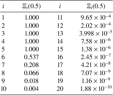
Example 3.1. For the parameter values $\lambda = 1, \mu = 1/3, \theta = 1/4, k = 5$ and $\ell = 20$ , Table 1 presents the values of $\Xi _{i}(0.5)$ , that is, the probability of serving a customer in $0.5$ time units given that they arrive in position i in the system.

Table 1

$\Xi _i(0.5)$ for $i \in \{1,2,\ldots , 20\}$ , $\lambda = 1, \mu = 1/3, \theta = 1/4, k = 5$ and $\ell = 20$ .

Table 1 Long description

The table is organized into four columns representing two sets of i and Xi sub i pairs.

First set (i from 1 to 10):

* i = 1, Xi sub i = 1.000

* i = 2, Xi sub i = 1.000

* i = 3, Xi sub i = 1.000

* i = 4, Xi sub i = 1.000

* i = 5, Xi sub i = 1.000

* i = 6, Xi sub i = 0.537

* i = 7, Xi sub i = 0.208

* i = 8, Xi sub i = 0.066

* i = 9, Xi sub i = 0.018

* i = 10, Xi sub i = 0.004

Second set (i from 11 to 20):

* i = 11, Xi sub i = 9.65 times 10 super minus 4

* i = 12, Xi sub i = 2.02 times 10 super minus 4

* i = 13, Xi sub i = 3.998 times 10 super minus 5

* i = 14, Xi sub i = 7.58 times 10 super minus 6

* i = 15, Xi sub i = 1.38 times 10 super minus 6

* i = 16, Xi sub i = 2.45 times 10 super minus 7

* i = 17, Xi sub i = 4.21 times 10 super minus 8

* i = 18, Xi sub i = 7.07 times 10 super minus 9

* i = 19, Xi sub i = 1.16 times 10 super minus 9

* i = 20, Xi sub i = 1.88 times 10 super minus 10

As expected, the probability of being served within $0.5$ time units is 1 when the tagged caller is in position less than or equal to k, it drops to $0.537$ when the tagged caller is in position $k+1$ and decreases further as the position of the tagged caller in the system increases.

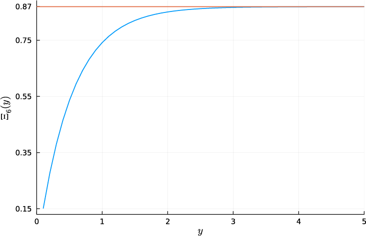
For the same set of parameter values, Figure 1 shows the plot of $\Xi _6(y)$ against y. The function $\Xi _6(y)$ gives the probability that a caller who arrives in position $6$ in the system is served within y time units. Its limiting value, which represents the probability that they are eventually served, is $0.87$ . This implies an abandonment probability of $0.13$ .

Figure 1

Plot of $\Xi _6(y)$ , the probability that a caller in position $6$ in the system is served within y time units.

4 The abandonment probability of a tagged caller

Using the second interpretation from Section 3.1, the abandonment probability for the tagged caller can be derived. For now, assume that the customers ahead of the tagged caller may abandon, but the tagged caller does not abandon when defining its waiting time. Let $\mathcal {W}_i$ denote the waiting time of a customer initially in position i under this modified system.

Under this assumption, the expression for the LST in (3.2) becomes

(4.1) $$ \begin{align} \mathbb{E}(e^{-s \mathcal{W}_i}) = \prod_{j = k+1}^{i} \frac{(j - 1 - k)\theta + k\mu}{(j - 1 - k)\theta + k\mu + s}. \end{align} $$

The change in the denominator reflects the fact that the tagged caller is not exposed to abandonment when computing this transform.

Now, introduce an independent exponential random variable $\mathcal {K}$ with rate s. Then,

$$ \begin{align*} \mathbb{P}(\mathcal{W}_i < \mathcal{K}) = \mathbb{E}(e^{-s \mathcal{W}_i}), \end{align*} $$

since $\mathcal {K}$ is independent of $\mathcal {W}_i$ .

Setting $s=\theta $ gives the tagged customer an independent exponential patience clock with the original system abandonment rate. Substituting $s=\theta $ in (4.1) yields a telescoping product that simplifies to

$$ \begin{align*} \frac{k\mu}{(i-k)\theta+k\mu}, \end{align*} $$

which is the probability that a customer who enters in position i is eventually served.

The probability that a tagged customer abandons the system, given that they arrive in position i, can also be computed directly. Let $\zeta _i$ denote this probability.

For positions where the customer is served immediately,

(4.2) $$ \begin{align} \zeta_i = 0. \end{align} $$

For positions with strictly positive waiting time, a first-step analysis is again used. At the first step, two outcomes are possible—either the tagged customer abandons immediately or they move one position closer to service. This gives the recursion

$$ \begin{align*} \zeta_i = \frac{\theta}{(i-k)\theta + k\mu} + \frac{(i-1-k)\theta + k\mu}{(i-k)\theta + k\mu}\zeta_{i-1}. \end{align*} $$

This can be rewritten as

$$ \begin{align*} 1 - \zeta_i = \frac{(i-1-k)\theta + k\mu}{(i-k)\theta + k\mu}(1 - \zeta_{i-1}). \end{align*} $$

Iterating this recursion from i down to k and using $1 - \zeta _k = 1$ from (4.2) yields the telescoping product

$$ \begin{align*} 1 - \zeta_i = \prod_{j=k+1}^{i} \frac{(j-1-k)\theta + k\mu}{(j-k)\theta + k\mu} = \frac{k\mu}{(i-k)\theta + k\mu}, \end{align*} $$

which is the same as (4.1). Hence, the probability that a tagged customer in position $i> k$ eventually abandons is

(4.3) $$ \begin{align} \zeta_i = \frac{(i-k)\theta}{(i-k)\theta + k\mu}. \end{align} $$

The expressions in (4.3) and (4.1) are of interest because they show that the probability that a customer in position i abandons before being served is identical to the probability that the first event after they enter the queue is an abandonment.

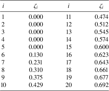
Example 4.1. The values for $\zeta _i$ for $i \in \{1,2,\ldots ,20\}$ are presented in Table 2 for the parameter values $\lambda = 1$ , $\mu = 1/3$ , $\theta = 1/4$ , $k = 5$ and $\ell = 20$ . The values imply that when the tagged caller is sixth in the system, the probability of abandonment is $0.130$ (consistent with the value obtained from Figure 1). If the tagged caller is seventh in the system, this probability increases to $0.231$ and it continues to rise as the position moves further back.

Table 2

$\zeta _i$ for $i \in \{1,2,\ldots , 20\}$ and the parameter values $\lambda = 1, \mu = 1/3, \theta = 1/4, k = 5$ and $\ell = 20$ .

Table 2 Long description

The table presents numerical values for zeta sub i across 20 iterations.

For the first set of indices (i from 1 to 10):

* i = 1, zeta sub i = 0.000

* i = 2, zeta sub i = 0.000

* i = 3, zeta sub i = 0.000

* i = 4, zeta sub i = 0.000

* i = 5, zeta sub i = 0.000

* i = 6, zeta sub i = 0.130

* i = 7, zeta sub i = 0.231

* i = 8, zeta sub i = 0.310

* i = 9, zeta sub i = 0.375

* i = 10, zeta sub i = 0.429

For the second set of indices (i from 11 to 20):

* i = 11, zeta sub i = 0.474

* i = 12, zeta sub i = 0.512

* i = 13, zeta sub i = 0.545

* i = 14, zeta sub i = 0.574

* i = 15, zeta sub i = 0.600

* i = 16, zeta sub i = 0.623

* i = 17, zeta sub i = 0.643

* i = 18, zeta sub i = 0.661

* i = 19, zeta sub i = 0.677

* i = 20, zeta sub i = 0.692

The data shows that zeta sub i remains at zero for the first five indices and then increases monotonically from i = 6 through i = 20.

5 Time-dependent transition probabilities

A method for computing transient transition probabilities is illustrated in this section. Together with the results in Sections 3–4, this allows us to answer questions such as, given the initial state of the system, what is the probability that a customer arriving at time t will abandon or be served within a specified time period.

For this, the original Markov chain $Y(t)$ defined in Section 2 is considered.

If $P^{(t)} = [p_{i_0,j}(t)]_{i_0,j \in S_y}$ is the probability matrix for the Markov chain $Y(t)$ and Q is the generator matrix, then the aim is to find an expression for $P^{(t)} = \exp (tQ)$ [Reference Borovkov8].

Let $p_{i_0,j}(t) = 0$ whenever $i_0 \notin S_y$ or $j \notin S_y$ . Let the total rate of the system at state $i_0$ be denoted by $\kappa (i_0)$ , then $\kappa (i_0) = \lambda \mathbb {1}_{i_0<\ell }+(\min (i_0,k)\mu + \max (0,i_0-k)\theta )\mathbb {1}_{i_0>0}$ . For $i_0,j \in S_y$ , the forward Kolmogorov equations are

$$ \begin{align*} \frac{dp_{i_0,j}(t)}{dt} = \lambda p_{i_0,j-1}(t) + (\max(0,j+1-k)\theta + \min(j+1,k)\mu)p_{i_0,j+1}(t) - \kappa(j)p_{i_0,j}(t). \end{align*} $$

Taking Laplace transforms on both sides yields

$$ \begin{align*} s\tilde{p}_{i_0,j}(s) - p_{i_0,j}(0) &= \lambda\tilde{p}_{i_0,j-1}(s) + (\max(0,j+1-k)\theta + \min(j+1,k)\mu)\tilde{p}_{i_0,j+1}(s) \\ &\quad - \kappa(j)\tilde{p}_{i_0,j}(s) \end{align*} $$

and $p_{i_0,j}(0) = \mathbb {1}_{i_0 = j}$ . Rearranging gives

$$ \begin{align*} \tilde{p}_{i_0,j}(s) = \dfrac{\lambda\tilde{p}_{i_0,j-1}(s) + (\max(0,j+1-k)\theta + \min(j+1,k)\mu)\tilde{p}_{i_0,j+1}(s) + \mathbb{1}_{i_0 = j}}{\kappa(j)+s}. \end{align*} $$

The system can be written in matrix form as

$$ \begin{align*} \boldsymbol{A} \tilde{\boldsymbol{p}}_{i_0} = \boldsymbol{b}_{i_0}, \end{align*} $$

where

$$ \begin{align*} \tilde{\boldsymbol{p}}_{i_0} = \begin{pmatrix} \tilde{p}_{i_0,0}(s) \\[1ex] \tilde{p}_{i_0,1}(s) \\[1ex] \tilde{p}_{i_0,2}(s) \\[1ex] \vdots \\[0.5ex] \tilde{p}_{i_0,\ell}(s) \end{pmatrix}, \qquad \boldsymbol{b}_{i_0} = \begin{pmatrix} \mathbb{1}_{i_0=0} \\[1ex] \mathbb{1}_{i_0=1} \\[1ex] \mathbb{1}_{i_0=2} \\[1ex] \vdots \\[0.5ex] \mathbb{1}_{i_0=\ell} \end{pmatrix}. \end{align*} $$

The tridiagonal matrix $\boldsymbol {A}$ has entries

$$ \begin{align*}A_{j,j} = \kappa(j) + s\quad \text{and}\quad A_{j,j-1} = -\lambda\end{align*} $$

for $j \ge 1$ , and

$$ \begin{align*}A_{j,j+1} = -(\max(0,j+1-k)\theta + \min(j+1,k)\mu)\end{align*} $$

for $j \le \ell -1$ , with all other entries equal to zero. Explicitly, it can be displayed as

$$ \begin{align*} \boldsymbol{A} = \begin{pmatrix} \kappa(0)+s & -(\theta \cdot \max(0,1-k) + \mu \cdot \min(1,k)) & \cdots & 0 \\ -\lambda & \kappa(1)+s & \cdots & 0 \\ 0 & -\lambda & \cdots & 0 \\ \vdots & \vdots & \ddots & \vdots \\ 0 & 0 & \cdots & \kappa(\ell)+s \end{pmatrix}. \end{align*} $$

Since $\boldsymbol {A}$ is tridiagonal, the linear system can be solved using a tridiagonal solver based on the Thomas algorithm [Reference Quarteroni, Sacco and Saleri17]. It provides a computational improvement compared with general matrix inversion, particularly for large values of $\ell $ .

Then, $\tilde p_{i_0,j}(s)$ can be inverted using the Euler method [Reference Abate and Whitt2] to obtain the transition probabilities.

In the Euler inversion algorithm, the Laplace transform must be evaluated at complex values of the Laplace parameter of the form

$$ \begin{align*} s_r = \dfrac{A + 2r\pi \iota}{2t}, \quad r = 0,1,\ldots,n+m+1. \end{align*} $$

Accordingly, the coefficients of the tridiagonal system become complex-valued, but the Thomas algorithm applies without modification since it only involves addition, multiplication and division operations, which are well defined for complex numbers. All computations are performed using complex double-precision arithmetic.

The parameters used in the Euler inversion follow the recommendations of [Reference Abate and Whitt2]. Specifically, $A = 18.4, n = 15$ and $m = 11$ .

The truncation level n determines the number of terms used in the initial alternating series, while m specifies the number of additional terms used in the Euler step. The error is estimated using the difference between successive Euler approximations, $|E(m,n+1,t)-E(m,n,t)|$ , and this quantity is used as an indicator of truncation accuracy.

For Example 5.1, the resulting error estimates decrease rapidly and are of the order of $10^{-10}$ in the early iterations and eventually reach magnitudes around $10^{-17}$ . This indicates that the numerical inversion is accurate and that the truncation levels $n=15$ and $m=11$ are sufficient for the parameter values considered.

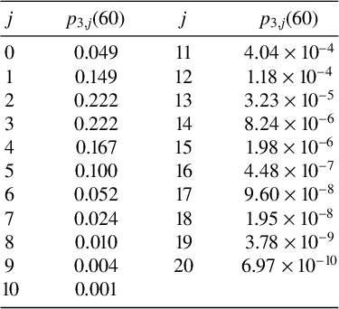
Example 5.1. Table 3 presents the values of $p_{3,j}(60)$ for the parameter values ${\lambda = 1, \mu = 1/3, \theta = 1/4, k = 5}$ and $\ell = 20$ , that is, the probability mass function for the state of the call centre at $t = 60$ , given the call centre has $3$ customers at time $0$ . Note that the probabilities sum to approximately one (up to numerical rounding), confirming the consistency of the numerical inversion procedure.

Table 3

$p_{3,j}(60)$ for the parameter values $\lambda = 1, \mu = 1/3, \theta = 1/4, k = 5$ and $\ell = 20$ .

Table 3 Long description

The table is organized into two main vertical sections, each containing columns for the index j and the corresponding value p sub (3,j) (60).

First section (j from 0 to 10):

* j = 0, p sub (3,j) (60) = 0.049

* j = 1, p sub (3,j) (60) = 0.149

* j = 2, p sub (3,j) (60) = 0.222

* j = 3, p sub (3,j) (60) = 0.222

* j = 4, p sub (3,j) (60) = 0.167

* j = 5, p sub (3,j) (60) = 0.100

* j = 6, p sub (3,j) (60) = 0.052

* j = 7, p sub (3,j) (60) = 0.024

* j = 8, p sub (3,j) (60) = 0.010

* j = 9, p sub (3,j) (60) = 0.004

* j = 10, p sub (3,j) (60) = 0.001

Second section (j from 11 to 20):

* j = 11, p sub (3,j) (60) = 4.04 times 10 super -4

* j = 12, p sub (3,j) (60) = 1.18 times 10 super -4

* j = 13, p sub (3,j) (60) = 3.23 times 10 super -5

* j = 14, p sub (3,j) (60) = 8.24 times 10 super -6

* j = 15, p sub (3,j) (60) = 1.98 times 10 super -6

* j = 16, p sub (3,j) (60) = 4.48 times 10 super -7

* j = 17, p sub (3,j) (60) = 9.60 times 10 super -8

* j = 18, p sub (3,j) (60) = 1.95 times 10 super -8

* j = 19, p sub (3,j) (60) = 3.78 times 10 super -9

* j = 20, p sub (3,j) (60) = 6.97 times 10 super -10

These values imply that if there are 3 customers in the system at the start, the probability of finding the call centre empty at $t = 60$ is $0.049$ , the probability of finding one customer in the system is $0.149$ and so on.

To validate the Laplace inversion procedure [Reference Abate and Whitt2], the transient state probabilities are also computed by calculating the matrix exponential of the generator matrix. For the finite-state system considered, the inversion-based results matched the direct computation with a maximum absolute error of order $10^{-9}$ .

Now, let $P_{i_0}(y,t)$ denote the probability that a caller arriving at time t is served within y time units, conditional on there being $i_0$ customers in the system at time $0$ . The system has finite capacity $\ell $ , so if an arrival occurs when the system is already in state $\ell $ , the customer is blocked and is not included in the performance measure.

The probability $P_{i_0}(y,t)$ can be computed using the results in Sections 3 and 5 as follows:

$$ \begin{align*} P_{i_0}(y,t) = \sum_{j = 1}^{\ell} \Xi_{j}(y) p_{i_0,j-1}(t). \end{align*} $$

Here, $p_{i_0,j-1}(t)$ is the probability that the system is in state $j-1$ at time t, given that the initial state at time $0$ is $i_0$ , and $\Xi _{j}(y)$ is the probability that a customer is served within y time units, given that they are in position j in the system upon arrival.

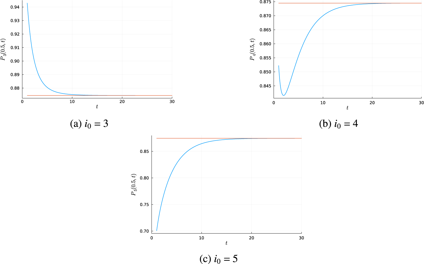
Figure 2 shows the plots of $P_{i_0}(y,t)$ against t for $y = 0.5$ and three different initial states $i_0 \in \{3,4,5\}$ .

Figure 2

Plot of $P_{i_0}(0.5,t)$ against t.

Figure 2 Long description

The figure consists of three panels labeled a, b, and c. Each panel features a blue curve representing a function and a horizontal red line representing an asymptote. The x-axis for all graphs is t, ranging from 0 to 30.

Panel a, labeled i sub 0 = 3, shows P sub 3 (0.5, t) on the y-axis ranging from 0.88 to 0.94. The blue curve starts at approximately 0.94 and exhibits a rapid exponential decay, converging to the red horizontal line at approximately 0.875 as t approaches 30.

Panel b, labeled i sub 0 = 4, shows P sub 4 (0.5, t) on the y-axis ranging from 0.845 to 0.875. The blue curve starts near 0.852, dips to a local minimum of approximately 0.842 around t = 2, and then increases asymptotically toward the red horizontal line at 0.874.

Panel c, labeled i sub 0 = 5, shows P sub 5 (0.5, t) on the y-axis ranging from 0.70 to 0.85. The blue curve starts at 0.70 and shows a steady concave-down increase, approaching the red horizontal line at approximately 0.875.

Three distinct behaviours corresponding to the different initial values are observed. For $i_0 = 3$ , the probability of service within $0.5$ time units decreases with t. For $i_0 = 4$ , the probability initially decreases for arrivals near time $0$ and subsequently increases. For $i_0 = 5$ , the probability increases over the entire range of t. In all cases, the curves converge to the same limiting value, corresponding to the stationary probability of being served within $0.5$ time units. The abandonment probability for a caller arriving at time t can be obtained in the same way and displays a similar but opposite trend.