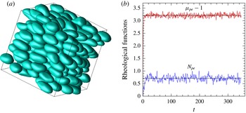
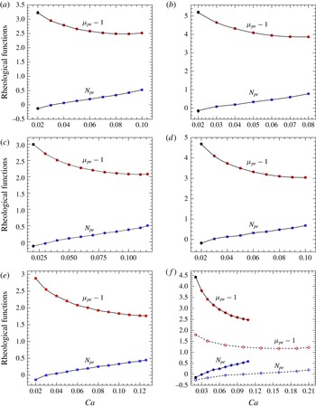
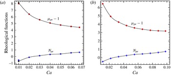
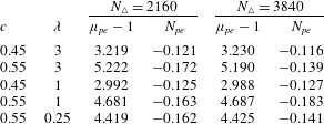
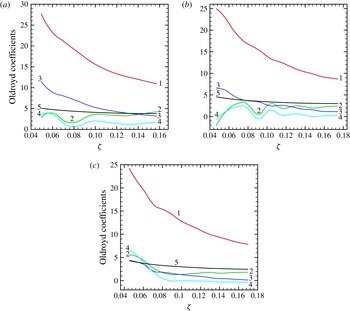
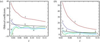
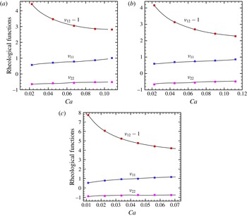
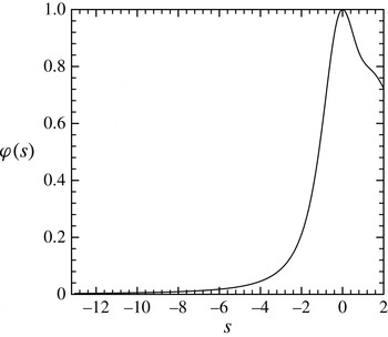
1 Introduction
Emulsions, i.e. dispersions of one immiscible liquid freely suspended in another liquid, represent an important class of non-Newtonian media encountered in many applications, including food and pharmaceutical industries, oil recovery and transportation. For any non-Newtonian liquid, it is essential to formulate a constitutive equation for the stress tensor valid in a broad class of kinematics. Knowing such an equation would allow solutions of boundary-value problems of non-Newtonian hydrodynamics in complex geometries of practical interest. For general large-strain flows, constitutive modelling is highly non-trivial because a non-Newtonian liquid is a material with fading memory, so that the stress depends on the whole prehistory of deformation of a material element. Rheological experiments alone, mostly limited to shear flows (steady or time dependent) are obviously not sufficient to aid in formulating a constitutive equation. A recent general approach to constitutive modelling oriented on numerical simulations (Martin, Zinchenko & Davis Reference Martin, Zinchenko and Davis2014) postulates an Oldroyd model with five variable coefficients. It was suggested therein to find these coefficients from fitting the model to the total of five rheological functions in the two steady base flows at arbitrary flow intensities. For unambiguous fitting, the Oldroyd parameters must depend on one instantaneous flow invariant. One base flow is traditional simple shear, with three viscometric functions (shear viscosity and first and second normal stress differences). The other base flow is planar extension (PE) (i.e. hyperbolic flow), with two extensiometric functions (extensional viscosity and the stress cross-difference). Since this modelling scheme assumes exact fitting to the rheology in two very distinct flows at arbitrary deformation rates, the resulting generalized Oldroyd model can be hoped to be reasonably accurate for flows with arbitrary kinematics encountered in the motion of a non-Newtonian liquid through complex geometries. This approach was tested in Martin et al. (Reference Martin, Zinchenko and Davis2014) for dilute emulsions of non-interacting, strongly deformable surfactant-free drops (with negligible inertia on the microscale). Here, the surface tension provides the fading memory mechanism. The boundary-integral (BI) method was used to both obtain the database rheological functions (to build the model) and precise results for selected general flows to be compared with the model predictions. The excess energy dissipation rate (from the drop-phase contribution) was found to be a better choice for the argument of the Oldroyd coefficients (compared to the more obvious choice of the second invariant of the rate-of-strain tensor). The model accurately predicted the drop-phase rheological response for a variety of test flows, both Lagrangian steady and unsteady, in a much wider range of flow intensities than do small-deformation theories.
The choice of simple shear and PE as the base flows in Martin et al. (Reference Martin, Zinchenko and Davis2014) was not accidental; this choice makes their constitutive modelling scheme applicable in principle to non-dilute systems (including concentrated emulsions, suspensions, etc.). With one exception (see below), these are the only flows allowing for reproducible periodic boundaries, and hence these flows are suitable for long-time numerical simulations with many drops, particles, etc. in a periodic cell. Without such periodic lattice reproducibility, excessive (exponentially fast) skewage of the periodic cell would destroy the numerical solution in a short time. For simple shear, lattice reproducibility is obvious and was heavily exploited before, including small-scale BI simulations for semi-dilute emulsions with up to 30 % drop volume fractions (Loewenberg & Hinch Reference Loewenberg and Hinch1996) and the first large-scale BI multidrop simulations for higher emulsion concentrations
 $c\leqslant 0.55$
(Zinchenko & Davis Reference Zinchenko and Davis2002, Reference Zinchenko, Davis and Petsev2004). Kraynik & Reinelt (Reference Kraynik and Reinelt1992) developed a non-trivial technique for lattice reproducibility in PE.
Zinchenko & Davis (Reference Zinchenko and Davis2015) (hereafter referred to as paper I) performed simulations by an improved, multipole-accelerated BI code with up to
 $N=400$
drops in a periodic cell, high resolution (up to
 $N_{\triangle }\sim 4000$
boundary elements per drop) and large strains up to
 ${\sim}10^{3}$
to significantly extend the steady shear-flow simulations of Zinchenko & Davis (Reference Zinchenko and Davis2002, Reference Zinchenko, Davis and Petsev2004) and study the viscometric functions in broad ranges of
 $c=0.45{-}0.55$
, drop-to-medium viscosity ratios
 $\unicode[STIX]{x1D706}=0.25{-}10$
and capillary numbers (with very small to large drop deformations). Extensiometric functions in steady PE were also simulated through the periodic boundary conditions of Kraynik & Reinelt (Reference Kraynik and Reinelt1992). These database rheological functions were used in the manner of Martin et al. (Reference Martin, Zinchenko and Davis2014) to build a generalized Oldroyd model with variable coefficients; limited model validations were also made. A major complication, compared to the case of dilute emulsions, is the gradual ‘phase transition’ to (partially) ordered flow in simple shear simulations observed after large strains and studied in detail in paper I. Below the transitional capillary number
 $Ca^{\ast }$
, it is practically impossible to reach convergence with the system size
 $N$
and make the results independent of the initial drop configuration; time averaging is also extremely challenging in that range. Moreover, even if unambiguous results could be obtained, they would still show a kinked behaviour, since the range
 $Ca<Ca^{\ast }$
obviously belongs to a different analytical branch. Decreasing
 $\unicode[STIX]{x1D706}$
strongly shifts
 $Ca^{\ast }$
to higher values. Transition to partially ordered flow was observed even at moderate concentrations
 $c=0.45$
, when
 $\unicode[STIX]{x1D706}=0.25$
. In contrast, flow-induced ordering never occurs in PE. When combining the viscometric and (always smooth) extensiometric functions for general constitutive modelling, the whole range
 $Ca<Ca^{\ast }$
had to be excluded from the shear-flow results, which makes such modelling restrictive, especially at small
 $\unicode[STIX]{x1D706}$
. One of the goals of the present study was to develop a more robust constitutive modelling scheme, without phase transition difficulties and the associated lower limitation on the range of flow intensities.
Another major limitation of paper I is the absence of surfactants in the rheological model. Practical emulsions are rarely clean, and even a small amount of contamination can have a strong effect on the rheology at high drop volume fractions, especially for slightly deformable drops near jamming conditions. To address this issue, a natural starting point is the model of an insoluble surfactant residing on the drop surfaces, valid if the mass exchange with the bulk is slow compared to the surfactant transport on the interfaces. Much work has been done by the BI method to explore the effects of surfactant on single drop deformation and break-up in axisymmetrical extensional flows (Stone & Leal Reference Stone and Leal1990; Milliken, Stone & Leal Reference Milliken, Stone and Leal1993; Pawar & Stebe Reference Pawar and Stebe1996; Eggleton & Stebe Reference Eggleton and Stebe1998; Eggleton, Pawar & Stebe Reference Eggleton, Pawar and Stebe1999; Eggleton, Tsai & Stebe Reference Eggleton, Tsai and Stebe2001) and shear flows (Li & Pozrikidis Reference Li and Pozrikidis1997; Yon & Pozrikidis Reference Yon and Pozrikidis1998; Bazhlekov, Anderson & Meijer Reference Bazhlekov, Anderson and Meijer2006). Some of these contributions assumed a linear equation for the surface tension
 $\unicode[STIX]{x1D70E}$
versus the surfactant concentration
 $\unicode[STIX]{x1D6E4}$
, strictly valid at small surface contaminations
 $\unicode[STIX]{x1D6E4}\ll \unicode[STIX]{x1D6E4}_{\infty }$
. The other studies used less idealized, nonlinear forms of
 $\unicode[STIX]{x1D70E}(\unicode[STIX]{x1D6E4})$
, relevant when
 $\unicode[STIX]{x1D6E4}$
can approach the maximum saturation
 $\unicode[STIX]{x1D6E4}_{\infty }$
(Milliken et al.
Reference Milliken, Stone and Leal1993; Pawar & Stebe Reference Pawar and Stebe1996; Eggleton & Stebe Reference Eggleton and Stebe1998; Eggleton et al.
Reference Eggleton, Pawar and Stebe1999, Reference Eggleton, Tsai and Stebe2001; Bazhlekov et al.
Reference Bazhlekov, Anderson and Meijer2006). In most of these papers, the Szyszkowski–Langmuir form of
 $\unicode[STIX]{x1D70E}(\unicode[STIX]{x1D6E4})$
was assumed. Eggleton et al. (Reference Eggleton, Tsai and Stebe2001) used this surfactant model to study the onset of tip streaming/dripping from a drop in elongational flow with
 $\unicode[STIX]{x1D706}=0.05$
and showed that the relevant critical capillary number
 $Ca_{cr}$
can be significantly less than
 $Ca_{cr}$
for a clean-drop break-up. In numerous single-drop BI simulations, there has been little emphasis, if at all, on the rheology; only Li & Pozrikidis (Reference Li and Pozrikidis1997), Yon & Pozrikidis (Reference Yon and Pozrikidis1998), Vlahovska, Loewenberg & Blawzdziewicz (Reference Vlahovska, Loewenberg and Bławzdziewicz2005) and Vlahovska, Bławzdziewicz & Loewenberg (Reference Vlahovska, Bławzdziewicz and Loewenberg2009) gave examples of the drop-phase contribution to the stress. Another nonlinear surfactant model is the Frumkin form with strong cohesive interactions (
 $\unicode[STIX]{x1D709}=-4$
) used to simulate drop motion in a tube (Johnson & Borhan Reference Johnson and Borhan1999). Here
 $\unicode[STIX]{x1D70E}(\unicode[STIX]{x1D6E4})$
has a plateau for
 $\unicode[STIX]{x1D6E4}$
well below
 $\unicode[STIX]{x1D6E4}_{\infty }$
not described by the Szyszkowski–Langmuir model. There appear to be no studies to explore how this vastly different form of
 $\unicode[STIX]{x1D70E}(\unicode[STIX]{x1D6E4})$
affects tip streaming/dripping and the related capillary numbers.
In the present work, general constitutive modelling is developed for highly concentrated emulsions of deformable drops with an insoluble surfactant through large-scale and high-resolution multidrop simulations. A linear model for
 $\unicode[STIX]{x1D70E}(\unicode[STIX]{x1D6E4})$
is assumed, which makes most sense when the surfactant is present as an impurity, not intentionally added (still allowing for strong effects on the rheology). Besides the fact that the linear model greatly reduces the large parameter space, it can be physically justified for a non-ionic surfactant, as long as the elasticity parameter
 $\unicode[STIX]{x1D6FD}$
stays within
 ${\sim}0.1$
(see § 6 for additional explanations). The surfactant transport is coupled to multidrop hydrodynamics through the convective–diffusive equation and the interfacial stress balance. However, only the limit of small surface diffusion is of interest, when this parameter no longer affects the rheology. The problem is formulated in § 2, including the non-dimensional parameters, implementation of periodic boundaries in multidrop simulations and the discussion of why simple shear must be excluded as an anomalous case from general constitutive modelling for highly concentrated emulsions. Instead, the present idea is to introduce a small but sufficient perturbation into the shear-flow kinematics to make it a planar mixed flow (PM), thus avoiding phase transition difficulties altogether. In § 3, we outline the highly efficient multipole-accelerated BI algorithm for multidrop simulations. The multipole part is the same as in the code of paper I for clean drops (and only briefly reviewed), but the presence of Marangoni stresses has required quite different BI desingularizations, as detailed in § 3.2 and the appendix A. In § 4, our simple algorithm for solving the convective–diffusive equation for
 $\unicode[STIX]{x1D6E4}$
on a triangulated surface is described, so are the difficulties limiting the range of capillary numbers for an effectively non-diffusing surfactant. In § 5, additional details of the algorithm are given. Steady-state database rheological functions obtained from multidrop simulations for PM and PE flows are discussed in §§ 6.1 and 6.2, respectively, including convergence analysis with the system size, surface resolution and the diffusion parameter. Comparison with some PE results from paper I for clean drops is also made. In § 7, we discuss necessary modifications of the constitutive modelling scheme from paper I (when the base simple shear has to be replaced by a PM flow) and the resulting Oldroyd coefficients. The validation tests of our constitutive model (although limited for concentrated emulsions) are presented in § 8. These include a steady PM flow with an intermediate flow parameter
 $\unicode[STIX]{x1D712}$
(much different from that for the base flow), and three time-dependent flows – PE and PM with variable deformation rates (transient and oscillatory).
As in paper I, all the simulations have been performed as single core on several multicore personal computers, with i7 4960X 3.6 GHz CPU being the fastest. With such limited resources, the high efficiency of our multipole acceleration still allowed for a large number of independent runs (necessary for a parametric analysis) by a serial code, thus avoiding communication bottlenecks typical of parallel computations. An alternative of running a simpler code (without multipole acceleration) on a massively parallel platform would be probably much less efficient, if feasible at all, for this kind of work.
2 Problem formulation
Consider an infinite set of three-dimensional, deformable Newtonian drops of viscosity
 $\unicode[STIX]{x1D707}^{\prime }$
freely suspended in a Newtonian liquid of viscosity
 $\unicode[STIX]{x1D707}_{e}=\unicode[STIX]{x1D707}^{\prime }/\unicode[STIX]{x1D706}$
and subject to a macroscopic flow
 $\boldsymbol{u}_{\infty }(\boldsymbol{x})=\unicode[STIX]{x1D735}\boldsymbol{u}_{\infty }\boldsymbol{\cdot }\boldsymbol{x}$
with a velocity gradient matrix
 $\unicode[STIX]{x1D735}\boldsymbol{u}_{\infty }$
. The drops are monodisperse, with the non-deformed radius
 $a_{o}$
, and small enough for Stokes equations to apply on the microscale for the fluid motion inside and outside the drops. The drops are still large enough for colloidal interactions and Brownian effects to be neglected. Under these conditions, accurate accounting of hydrodynamical interactions prohibits drop surface contact and coalescence (Yiantsios & Davis Reference Yiantsios and Davis1990, Reference Yiantsios and Davis1991). Each drop surface
 $S_{\unicode[STIX]{x1D6FC}}$
is covered with the same amount
 $$\begin{eqnarray}\displaystyle Q=\int _{S_{\unicode[STIX]{x1D6FC}}}\unicode[STIX]{x1D6E4}\,\text{d}S & & \displaystyle\end{eqnarray}$$
of an insoluble surfactant. A traditional, linear equation of state
 $\unicode[STIX]{x1D70E}=\unicode[STIX]{x1D70E}_{o}-RT\unicode[STIX]{x1D6E4}$
relates the local surface tension
 $\unicode[STIX]{x1D70E}$
and local surfactant concentration
 $\unicode[STIX]{x1D6E4}$
, with
 $\unicode[STIX]{x1D70E}_{o}$
being the clean surface value,
 $R$
the universal gas constant and
 $T$
the uniform absolute temperature. The linear equation of state is deemed appropriate (e.g. Eggleton et al.
Reference Eggleton, Pawar and Stebe1999) as long as the surfactant concentration
 $\unicode[STIX]{x1D6E4}$
does not approach the maximum packing limit
 $\unicode[STIX]{x1D6E4}_{\infty }$
(which also eliminates the complications of surface shear viscosity). In particular, this is the case when the surfactant is present as an impurity, not intentionally added (e.g. Eggleton et al.
Reference Eggleton, Pawar and Stebe1999). The surfactant transport on each drop surface obeys the convective–diffusive equation (e.g. Stone Reference Stone1990)
 $$\begin{eqnarray}\displaystyle \frac{\text{D}\unicode[STIX]{x1D6E4}}{\text{D}t}+\unicode[STIX]{x1D6E4}\unicode[STIX]{x1D735}_{s}\boldsymbol{\cdot }\boldsymbol{u}_{s}+2k\unicode[STIX]{x1D6E4}(\boldsymbol{u}\boldsymbol{\cdot }\boldsymbol{n})-\unicode[STIX]{x1D735}_{s}\boldsymbol{\cdot }(D_{s}\unicode[STIX]{x1D735}_{s}\unicode[STIX]{x1D6E4})=0. & & \displaystyle\end{eqnarray}$$
Here,
 $\text{D}/\text{D}t$
is the Lagrangian derivative along the trajectory of a fluid element moving with velocity
 $\boldsymbol{u}$
along the interface,
 $\boldsymbol{u}_{s}$
is the tangential part of
 $\boldsymbol{u}$
,
 $\boldsymbol{n}$
is the outward unit normal to
 $S_{\unicode[STIX]{x1D6FC}}$
,
 $k=(k_{1}+k_{2})/2$
is the local mean curvature of
 $S_{\unicode[STIX]{x1D6FC}}$
(the average of the two principal curvatures) consistent with the direction of
 $\boldsymbol{n}$
,
 $D_{s}$
is the surfactant diffusivity (assumed variable for technical reasons, see § 4), and
 $\unicode[STIX]{x1D735}_{s}$
is the surface gradient operator. The transport equation is often written in an alternative form, with partial derivative
 $\unicode[STIX]{x2202}\unicode[STIX]{x1D6E4}/\unicode[STIX]{x2202}t$
, but such a derivative does not have a clear meaning for a deformable surface, and so we prefer the rigorous, well-defined form (2.2). The surfactant transport (2.2) preserves the total amount of surfactant on each drop surface and is coupled to multidrop hydrodynamics through the interfacial stress balances (including the Marangoni stress
 $\unicode[STIX]{x1D735}_{s}\unicode[STIX]{x1D70E}$
). The characteristic surfactant concentration (as if it was uniformly distributed on spherical surfaces) is
 $\unicode[STIX]{x1D6E4}_{eq}=Q/(4\unicode[STIX]{x03C0}a_{o}^{2})$
. Accordingly, we define the elasticity parameter
 $\unicode[STIX]{x1D6FD}$
and the ‘equilibrium surface tension’ (e.g. Stone & Leal Reference Stone and Leal1990; Milliken et al.
Reference Milliken, Stone and Leal1993)
 $\unicode[STIX]{x1D70E}_{eq}$
:
 $$\begin{eqnarray}\displaystyle \unicode[STIX]{x1D6FD}=\frac{Q}{4\unicode[STIX]{x03C0}a_{o}^{2}}\frac{RT}{\unicode[STIX]{x1D70E}_{o}},\quad \unicode[STIX]{x1D70E}_{eq}=\unicode[STIX]{x1D70E}_{o}(1-\unicode[STIX]{x1D6FD}). & & \displaystyle\end{eqnarray}$$
(Our definition of
 $\unicode[STIX]{x1D6FD}$
should not be confused with the elasticity definitions in the literature based on
 $\unicode[STIX]{x1D6E4}_{\infty }$
for nonlinear equations of state
 $\unicode[STIX]{x1D70E}(\unicode[STIX]{x1D6E4})$
.) Surfactant diffusivities are subject to large uncertainties, but are generally deemed very small (e.g. Eggleton et al.
Reference Eggleton, Pawar and Stebe1999). For this reason, we are only interested in the regime of low diffusivities
 $D_{s}\rightarrow 0$
, when this parameter no longer affects the macroscopic properties of the emulsion.
At each time
 $t\geqslant 0$
, the infinite drop system is obtained from the basic configuration of
 $N\gg 1$
drops with surface centroids
 $\boldsymbol{x}_{1}^{c},\ldots ,\boldsymbol{x}_{N}^{c}$
in the basic cell
 $V$
by triply periodic continuation into the whole space with periods
 $\boldsymbol{e}_{1}$
,
 $\boldsymbol{e}_{2}$
,
 $\boldsymbol{e}_{3}$
; the cell
 $V=\{\unicode[STIX]{x1D709}^{i}\boldsymbol{e}_{i},0\leqslant \unicode[STIX]{x1D709}^{i}<1\}$
is the span of
 $\boldsymbol{e}_{1}$
,
 $\boldsymbol{e}_{2}$
and
 $\boldsymbol{e}_{3}$
. Periodic continuation into the whole space is paramount for reliable long-time simulations of macroscopic properties independent of the system size. Ideally, one would want to predict the emulsion rheology (namely, the macroscopic stress tensor) for an arbitrary history of the macroscopic velocity gradient
 $\unicode[STIX]{x1D735}\boldsymbol{u}_{\infty }(t)$
. However, it is possible to dynamically maintain such periodic continuation, with limited skewage of periodic cells, for only three types of macroscopic flow (i) simple shear
 $\boldsymbol{u}_{\infty }(\boldsymbol{x})=(\dot{\unicode[STIX]{x1D6FE}}x_{2},0,0)$
, (ii) PE flow
 $\boldsymbol{u}_{\infty }(\boldsymbol{x})=(\dot{\unicode[STIX]{x1D6E4}}x_{1},-\dot{\unicode[STIX]{x1D6E4}}x_{2},0)$
and (iii) PM flow
 $\boldsymbol{u}_{\infty }(\boldsymbol{x})=(\dot{\unicode[STIX]{x1D6FE}}_{m}x_{2},\dot{\unicode[STIX]{x1D6FE}}_{m}\unicode[STIX]{x1D712}x_{1},0)$
with the flow parameter
 $\unicode[STIX]{x1D712}\in (-1,1]$
; PE is equivalent to PM with
 $\unicode[STIX]{x1D712}=1$
. (Note that our notation
 $\dot{\unicode[STIX]{x1D6E4}}$
for the PE deformation rate should not be confused below with a time derivative of the surfactant concentration.)
For simple shear with constant
 $\dot{\unicode[STIX]{x1D6FE}}$
, maintaining periodic boundaries is straightforward and achieved by simple lattice restructuring at half-integer strains
 $\dot{\unicode[STIX]{x1D6FE}}t$
; such restructuring has been heavily exploited in prior simulations for emulsions (Loewenberg & Hinch Reference Loewenberg and Hinch1996; Zinchenko & Davis Reference Zinchenko and Davis2002, Reference Zinchenko, Davis and Petsev2004, paper I) and suspensions. The existence of reproducible lattices in PE found by Kraynik & Reinelt (Reference Kraynik and Reinelt1992) is non-trivial. Following their results for a ‘critical lattice’ (with minimum skewage), the initial periodic cell is chosen as a cube
 $L\times L\times L$
, with one side (along
 $\boldsymbol{e}_{1}$
) inclined at angle
 $\unicode[STIX]{x1D703}_{o}=\tan ^{-1}[(\sqrt{5}-1)/2]\approx 31.7^{\circ }$
to the
 $x_{1}$
-axis. Using
 $L$
as the length scale, the initial lattice vectors are
 $\boldsymbol{e}_{1}^{o}=(\cos \unicode[STIX]{x1D703}_{o},\sin \unicode[STIX]{x1D703}_{o},0)$
and
 $\boldsymbol{e}_{2}^{o}=(-\sin \unicode[STIX]{x1D703}_{o},\cos \unicode[STIX]{x1D703}_{o},0)$
. Choosing the Hencky strain period in a special way,
 $\unicode[STIX]{x1D700}_{p}=\ln [(3+\sqrt{5})/2]\approx 0.9624$
, the lattice reproducibility for a constant deformation rate
 $\dot{\unicode[STIX]{x1D6E4}}$
is achieved as follows. By
 $\dot{\unicode[STIX]{x1D6E4}}t=\unicode[STIX]{x1D700}_{p}/2$
, the lattice dynamics
 $\text{d}\boldsymbol{e}_{i}/\text{d}t=\text{diag}(\dot{\unicode[STIX]{x1D6E4}},-\dot{\unicode[STIX]{x1D6E4}},0)\boldsymbol{e}_{i}$
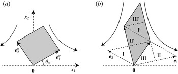
brings the basic periodic cell
 $V$
to a shape shown as the dashed-line parallelogram in figure 1. Switching to
 $\boldsymbol{e}_{1}+\boldsymbol{e}_{2}$
and
 $\boldsymbol{e}_{1}+2\boldsymbol{e}_{2}$
as the new lattice vectors
 $\boldsymbol{e}_{1}$
and
 $\boldsymbol{e}_{2}$
respectively, and integrating the lattice dynamics further to
 $\dot{\unicode[STIX]{x1D6E4}}t=\unicode[STIX]{x1D700}_{p}$
reproduces the initial cell, owing to the special choice of
 $\unicode[STIX]{x1D703}_{o}$
and
 $\unicode[STIX]{x1D700}_{p}$
. For detailed lattice dynamics in the Hencky strain interval of
 $\unicode[STIX]{x1D700}_{p}$
, see paper I. There is also a simple mapping (figure 1
b) between the old and new periodic cells at restructuring moments to recalculate the new drop positions.
Dynamics of the computational cell in steady PE; (a)
 $\dot{\unicode[STIX]{x1D6E4}}t=0$
, (b)
 $\dot{\unicode[STIX]{x1D6E4}}t=\unicode[STIX]{x1D700}_{p}/2$
. In (b), the cell is restructured (shaded area is the new cell) to continue the simulation. Mapping between the old and new cells (region I is translated to
 $\text{I}^{\prime }$
, etc.) is used in (b) to recalculate the new drop positions. The third dimension
 $x_{3}$
is not shown. Adapted from Zinchenko & Davis (Reference Zinchenko and Davis2015).

For a mixed flow with
 $\unicode[STIX]{x1D712}>0$
, a diagonalizing transformation
 $$\begin{eqnarray}\displaystyle \unicode[STIX]{x1D735}\boldsymbol{u}_{\infty }=\unicode[STIX]{x1D64E}\,\text{diag}(\dot{\unicode[STIX]{x1D6E4}},-\dot{\unicode[STIX]{x1D6E4}},0)\unicode[STIX]{x1D64E}^{-1} & & \displaystyle\end{eqnarray}$$
was found by Hunt, Bernardi & Todd (Reference Hunt, Bernardi and Todd2010) to relate the PM velocity gradient to that for some auxiliary PE, with a real valued matrix
 $\unicode[STIX]{x1D64E}$
. With the present definition
 $\boldsymbol{u}_{\infty }(\boldsymbol{x})=\dot{\unicode[STIX]{x1D6FE}}_{m}(x_{2},\unicode[STIX]{x1D712}x_{1},0)$
of the mixed flow,
 $\dot{\unicode[STIX]{x1D6E4}}=\dot{\unicode[STIX]{x1D6FE}}_{m}\sqrt{\unicode[STIX]{x1D712}}$
and the matrices
 $\unicode[STIX]{x1D64E}=\unicode[STIX]{x1D64E}(\unicode[STIX]{x1D712})$
and
 $\unicode[STIX]{x1D64E}^{-1}$
are given explicitly by (2.6) of paper I. According to (2.4), lattice reproducibility for steady PM is simply reduced to the case of Kraynik & Reinelt (Reference Kraynik and Reinelt1992). Indeed, the required lattice dynamics
 $\text{d}\boldsymbol{e}_{i}/\text{d}t=\unicode[STIX]{x1D735}\boldsymbol{u}_{\infty }\boldsymbol{\cdot }\boldsymbol{e}_{i}$
is equivalent to
 $\text{d}\widetilde{\boldsymbol{e}}_{i}/\text{d}t=\text{diag}(\dot{\unicode[STIX]{x1D6E4}},-\dot{\unicode[STIX]{x1D6E4}},0)\widetilde{\boldsymbol{e}}_{i}$
for auxiliary vectors
 $\widetilde{\boldsymbol{e}}_{i}=\unicode[STIX]{x1D64E}^{-1}\boldsymbol{e}_{i}$
. Restructuring transformation
 $(\widetilde{\boldsymbol{e}}_{1},~\widetilde{\boldsymbol{e}}_{2})\rightarrow (\widetilde{\boldsymbol{e}}_{1}+\widetilde{\boldsymbol{e}}_{2},~\widetilde{\boldsymbol{e}}_{1}+2\widetilde{\boldsymbol{e}}_{2})$
to the new basis vectors in the PE flow space at half-integer values of
 $\dot{\unicode[STIX]{x1D6E4}}t/\unicode[STIX]{x1D700}_{p}$
begets the same transformation of the lattice vectors
 $\boldsymbol{e}_{i}=\unicode[STIX]{x1D64E}\widetilde{\boldsymbol{e}}_{i}$
. For weak mixed flows (
 $\unicode[STIX]{x1D712}<0$
), the lattice dynamics of
 $\boldsymbol{e}_{1}(t)$
and
 $\boldsymbol{e}_{2}(t)$
is periodic and does not require restructuring at all (although difficulties would arise at very small
 $|\unicode[STIX]{x1D712}|$
). However, the case
 $\unicode[STIX]{x1D712}<0$
is less relevant to non-Newtonian hydrodynamics (as shown in paper I) and is not of interest in the present work.
The above lattice reproducibility techniques are easily extended to time-dependent simple shear, PE and PM, with sign-definite deformation rates
 $\dot{\unicode[STIX]{x1D6FE}}(t)$
,
 $\dot{\unicode[STIX]{x1D6E4}}(t)$
and
 $\dot{\unicode[STIX]{x1D6FE}}_{m}(t)$
. For example, the lattice vector dynamics for time-dependent PE can be written in the Kraynik–Reinelt’s form
 $\text{d}\boldsymbol{e}_{i}/\text{d}\widehat{t}=\text{diag}(1,-1,0)\boldsymbol{e}_{i}$
using the artificial time
 $\widehat{t}$
defined by
 $\text{d}\widehat{t}=\dot{\unicode[STIX]{x1D6E4}}\text{d}t$
. We are not aware, however, of any types of flow, other than simple shear, PE and PM, with lattice reproducibility.
Despite the limited number of choices for macroscopic flow which can be reliably simulated with periodic boundaries, these flows can be used as a database to build and validate a general rheological model for highly concentrated emulsions with surfactant, deemed reasonably accurate for an arbitrary history of deformation of a material element. Specifically, we will combine the simulation results from two steady-state database flows to construct a constitutive equation for an arbitrary flow, either Lagrangian steady or unsteady.
Difficulties with simple shear as a database flow. A steady simple shear, although a staple flow in rheology, is a poor choice as a database flow for highly concentrated emulsions (and probably many other microstructurally complex fluids with strong interactions between the inclusions), since it comes with substantial limitations. It was demonstrated by multidrop simulations for clean drops in paper I that, at large enough drop volume fractions
 $c$
and small enough capillary numbers
 $Ca=\unicode[STIX]{x1D707}_{e}\dot{\unicode[STIX]{x1D6FE}}a_{o}/\unicode[STIX]{x1D70E}$
, an emulsion transitions from disordered to partially ordered flow with layers of drops sliding past each other, if the simulation is run for sufficiently large strains
 $\dot{\unicode[STIX]{x1D6FE}}t$
(figure 18 of paper I). Obviously, this ‘phase transition’ is the emulsion response to jamming (at sufficiently small drop deformations), as it eventually finds an easier way to flow in an ordered fashion and with a smaller effective viscosity. Accordingly, in such simulations, there is an extremely slow relaxation of the viscometric functions (the emulsion shear viscosity and normal stress differences) to statistical steady state. For example, at
 $c=0.55$
,
 $\unicode[STIX]{x1D706}=1$
,
 $Ca=0.05$
and
 $N=400$
drops, large initial strains of
 $\dot{\unicode[STIX]{x1D6FE}}t\sim 600{-}700$
have to be excluded from averaging. Unambiguous and well-behaved time-averaged results are only achieved above the transition point (which is
 $Ca\approx 0.075$
for
 $c=0.55$
and
 $\unicode[STIX]{x1D706}=1$
). Below the transitional
 $Ca$
, the steady-state results are strongly sensitive to the system size (even with
 $N=400$
drops) and to the choice of the initial drop configuration (figure 15c of paper I). Even if these severe ergodic difficulties could be overcome, the steady-state viscometric functions would still show kinked behaviour versus
 $Ca$
, since they represent a different analytical branch below the transitional
 $Ca$
. Reducing the viscosity ratio
 $\unicode[STIX]{x1D706}$
strongly shifts the transition to larger capillary numbers. While for
 $c=0.55$
and
 $\unicode[STIX]{x1D706}=1$
, only the
 $Ca<0.075$
results are unsatisfying, for
 $\unicode[STIX]{x1D706}=0.25$
the steady-state normal stress differences suffer from uncertainties in a much wider range
 $Ca<0.19{-}0.22$
. At this small
 $\unicode[STIX]{x1D706}$
, transition to ordered flow is observed even for drop volume fractions as low as
 $c=0.45$
, when
 $Ca<0.18$
. Thus, if steady simple shear is chosen as database flow, a large range of flow intensities would have to be excluded from constitutive modelling.
None of these difficulties was observed in our clean-drop simulations (paper I) for PE and PM (with
 $\unicode[STIX]{x1D712}=0.25$
). Namely, in the whole range of
 $c\leqslant 0.55$
explored, relaxation to the statistical steady state is always fast, the time-averaged steady-state results for rheological functions are independent of initial conditions, rapidly convergent with the system size (when
 $N\sim 100$
) and show smooth dependence on the deformation rate, regardless of
 $\unicode[STIX]{x1D706}$
and the degree of drop deformation. The absence of phase transition to order in such flows can be possibly explained by the absence of the geometric picture allowing layers of drops to slide past each other in an ordered fashion.
Leaving aside exceptional cases (e.g. straight pipe/channel flows), fluid motion through a complex geometry is never of a steady simple shear type. The absence of phase transition to order in general flows makes simple shear, therefore, an anomalous case and an unsuitable (or at least, restrictive) building block for general rheology.
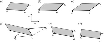
The geometry of the computational cell in steady PM flow (
 $\unicode[STIX]{x1D712}=0.16$
) at
 $\dot{\unicode[STIX]{x1D6FE}}_{m}t/\unicode[STIX]{x1D700}_{p}=0$
(a), 0.417 (b), 0.833 (c), 1.25 (d), 1.667 (e) and 2.083 (f). In (d), the cell is restructured (shaded area is the new cell) to continue the simulation. At
 $\dot{\unicode[STIX]{x1D6FE}}_{m}t/\unicode[STIX]{x1D700}_{p}=5/2$
(not shown), the initial periodic cell is reproduced.

The same considerations should apply to highly concentrated emulsions of drops with surfactant (and, of course, other non-Newtonian liquids). Accordingly, instead of simple shear, our first database flow is steady PM with a moderately small
 $\unicode[STIX]{x1D712}>0$
. The choice
 $\unicode[STIX]{x1D712}=0.16$
was found to be a sufficient perturbation to avoid any phase transition difficulties, with acceptable skewage of periodic cells during simulations (figure 2). This PM gives steady-state non-dimensional rheological functions defined through the deviatoric part
 $\unicode[STIX]{x1D64F}=\unicode[STIX]{x1D72E}-(1/3)\text{tr}(\unicode[STIX]{x1D72E})\unicode[STIX]{x1D644}$
of the macroscopic stress tensor
 $\unicode[STIX]{x1D72E}$
:
 $$\begin{eqnarray}\displaystyle \unicode[STIX]{x1D708}_{ij}=\frac{T_{ij}}{\unicode[STIX]{x1D707}_{e}\dot{\unicode[STIX]{x1D6FE}}_{m}(\unicode[STIX]{x1D712}+1)}. & & \displaystyle\end{eqnarray}$$
Of these, only three (
 $\unicode[STIX]{x1D708}_{12}$
,
 $\unicode[STIX]{x1D708}_{11}$
and
 $\unicode[STIX]{x1D708}_{22}$
) are independent;
 $\unicode[STIX]{x1D708}_{12}$
is the non-dimensional mixed-flow viscosity.
As in paper I, the second database flow is steady-state PE
 $\boldsymbol{u}_{\infty }(\boldsymbol{x})=(\dot{\unicode[STIX]{x1D6E4}}x_{1},-\dot{\unicode[STIX]{x1D6E4}}x_{2},0)$
, which gives two more rheological functions – the non-dimensional PE flow viscosity
 $\unicode[STIX]{x1D707}_{pe}$
and the stress cross-difference
 $N_{pe}$
:
 $$\begin{eqnarray}\displaystyle \unicode[STIX]{x1D707}_{pe}=\frac{\unicode[STIX]{x1D6F4}_{11}-\unicode[STIX]{x1D6F4}_{22}}{4\unicode[STIX]{x1D707}_{e}\dot{\unicode[STIX]{x1D6E4}}},\quad N_{pe}=\frac{\unicode[STIX]{x1D6F4}_{11}+\unicode[STIX]{x1D6F4}_{22}-2\unicode[STIX]{x1D6F4}_{33}}{4\unicode[STIX]{x1D707}_{e}\dot{\unicode[STIX]{x1D6E4}}}. & & \displaystyle\end{eqnarray}$$
The capillary number is defined in general through the second invariant
 $I_{2}=\text{tr}(\unicode[STIX]{x1D640}_{\infty }^{2})$
of the rate-of-strain tensor
 $\unicode[STIX]{x1D640}_{\infty }$
for the macroscopic flow
 $\boldsymbol{u}_{\infty }$
and the equilibrium surface tension (2.3):
 $$\begin{eqnarray}\displaystyle Ca=\unicode[STIX]{x1D707}_{e}(2I_{2})^{1/2}a_{o}/\unicode[STIX]{x1D70E}_{eq}. & & \displaystyle\end{eqnarray}$$
In particular,
 $Ca=2\unicode[STIX]{x1D707}_{e}\dot{\unicode[STIX]{x1D6E4}}a_{o}/\unicode[STIX]{x1D70E}_{eq}$
for PE and
 $Ca=(1+\unicode[STIX]{x1D712})\unicode[STIX]{x1D707}_{e}\dot{\unicode[STIX]{x1D6FE}}_{m}a_{o}/\unicode[STIX]{x1D70E}_{eq}$
for PM flows, respectively. The present work seeks to accurately obtain the database rheological functions (2.5) and (2.6) for highly concentrated emulsions from multidrop simulations, study their dependence on the microstructural parameters
 $c$
,
 $\unicode[STIX]{x1D706}$
,
 $Ca$
and
 $\unicode[STIX]{x1D6FD}$
, use these functions to build a general rheological model for arbitrary kinematics and validate this model.
3 Multipole-accelerated boundary-integral solution
3.1 Boundary-integral equations
Like in paper I, highly efficient multipole-accelerated boundary-integral techniques are used to solve the hydrodynamical multidrop problem at each time step, given the surface tension distributions on the drop surfaces. For either of the database flows, the length scale
 $L$
is defined as in § 2, the time scale is
 $(2I_{2})^{-1/2}$
and the velocity scale is
 $(2I_{2})^{1/2}L$
. The non-dimensional periodic cell
 $V$
has unit volume at all times. The surface tension is scaled with
 $\unicode[STIX]{x1D70E}_{eq}$
. The non-dimensional system of BI equations for the fluid velocity
 $\boldsymbol{u}(\boldsymbol{y})$
on drop surfaces
 $S_{\unicode[STIX]{x1D6FC}}$
to be solved iteratively is written as
 $$\begin{eqnarray}\displaystyle \boldsymbol{u}(\boldsymbol{y}) & = & \displaystyle \frac{(\unicode[STIX]{x1D706}-1)}{(\unicode[STIX]{x1D706}+1)}\left[2\mathop{\sum }_{\unicode[STIX]{x1D6FD}=1}^{N}\int _{S_{\unicode[STIX]{x1D6FD}}}\boldsymbol{Q}(\boldsymbol{x})\boldsymbol{\cdot }\widetilde{\unicode[STIX]{x1D749}}(\boldsymbol{x}-\boldsymbol{y})\boldsymbol{\cdot }\boldsymbol{n}(\boldsymbol{x})\,\text{d}S_{x}+\langle \boldsymbol{u}\rangle _{\unicode[STIX]{x1D6FC}}\right.\nonumber\\ \displaystyle & & \displaystyle +\,\left.2\mathop{\sum }_{\unicode[STIX]{x1D6FD}=1}^{N}\int _{S_{\unicode[STIX]{x1D6FD}}}(\boldsymbol{Q}\boldsymbol{\cdot }\boldsymbol{n})(\boldsymbol{x}-\boldsymbol{x}_{\unicode[STIX]{x1D6FD}}^{c})\,\text{d}S_{x}\right]+\boldsymbol{F}(\boldsymbol{y}),\quad \boldsymbol{y}\in S_{\unicode[STIX]{x1D6FC}}.\end{eqnarray}$$
(Here and in the rest of § 3, the index
 $\unicode[STIX]{x1D6FD}$
should not be confused with the elasticity parameter (2.3).) Except for the expression for the inhomogeneous term
 $\boldsymbol{F}(\boldsymbol{y})$
(see below), (3.1) is identical to the one used in paper I for clean drops. In particular, velocity fluctuations
 $\boldsymbol{Q}(\boldsymbol{x})=\boldsymbol{u}(\boldsymbol{x})-\langle \boldsymbol{u}\rangle _{\unicode[STIX]{x1D6FD}}$
from the surface-averaged values
 $\langle \boldsymbol{u}\rangle _{\unicode[STIX]{x1D6FD}}$
are used on
 $S_{\unicode[STIX]{x1D6FD}}$
instead of
 $\boldsymbol{u}(\boldsymbol{x})$
to significantly reduce the integrand variations and thereby accelerate convergence in the most difficult, multipole part of the algorithm. Instead of the fundamental stresslet
 $\unicode[STIX]{x1D749}(\boldsymbol{r})$
in the double-layer integrals (3.1), we work with the auxiliary third-rank tensor
 $\widetilde{\unicode[STIX]{x1D749}}(\boldsymbol{r})=\unicode[STIX]{x1D749}(\boldsymbol{r})-\boldsymbol{r}\unicode[STIX]{x1D644}$
which is (unlike
 $\unicode[STIX]{x1D749}$
) triply periodic and fully symmetric in all three indices (Zinchenko & Davis Reference Zinchenko and Davis2000, Reference Zinchenko and Davis2002, Reference Zinchenko and Davis2003, paper I).
The non-dimensional form of
 $\boldsymbol{F}(\boldsymbol{y})$
in the present problem takes into account the variable surface tension and the Marangoni stress in the interfacial stress jump condition:
 $$\begin{eqnarray}\displaystyle \boldsymbol{F}(\boldsymbol{y})=\frac{2}{\unicode[STIX]{x1D706}+1}\left[\boldsymbol{u}_{\infty }(\boldsymbol{y})+\mathop{\sum }_{\unicode[STIX]{x1D6FD}=1}^{N}\int _{S_{\unicode[STIX]{x1D6FD}}}\boldsymbol{f}(\boldsymbol{x})\boldsymbol{\cdot }\unicode[STIX]{x1D642}(\boldsymbol{x}-\boldsymbol{y})\,\text{d}S_{x}\right]. & & \displaystyle\end{eqnarray}$$
Here, the vector field
 $$\begin{eqnarray}\displaystyle \boldsymbol{f}(\boldsymbol{x})=\frac{a}{Ca}\{2[\unicode[STIX]{x1D70E}(\boldsymbol{x})k(\boldsymbol{x})-\langle \unicode[STIX]{x1D70E}k\rangle _{\unicode[STIX]{x1D6FD}}]\boldsymbol{n}(\boldsymbol{x})-\unicode[STIX]{x1D735}_{s}\unicode[STIX]{x1D70E}\}\quad (\boldsymbol{x}\in S_{\unicode[STIX]{x1D6FD}}) & & \displaystyle\end{eqnarray}$$
represents the stress jump on
 $S_{\unicode[STIX]{x1D6FD}}$
(the surface average of
 $\unicode[STIX]{x1D70E}k$
over
 $S_{\unicode[STIX]{x1D6FD}}$
is subtracted to reduce the variation of
 $\boldsymbol{f}$
without affecting the integrals (3.2)),
 $a=a_{o}/L$
is the non-dimensional non-deformed drop radius and
 $\unicode[STIX]{x1D642}$
is the triply periodic, symmetric second-rank tensor of Hasimoto (Reference Hasimoto1959). With our normalization, this tensor satisfies
 $$\begin{eqnarray}\displaystyle \unicode[STIX]{x1D6FB}^{2}\unicode[STIX]{x1D642}(\boldsymbol{x})-\unicode[STIX]{x1D735}\boldsymbol{q}(\boldsymbol{x})=\unicode[STIX]{x1D735}\boldsymbol{\cdot }\unicode[STIX]{x1D749}(\boldsymbol{x})=\mathop{\sum }_{\boldsymbol{m}}\unicode[STIX]{x1D6FF}(\boldsymbol{x}-\boldsymbol{P}(\boldsymbol{m}))\unicode[STIX]{x1D644}, & & \displaystyle\end{eqnarray}$$
where
 $\boldsymbol{q}(\boldsymbol{x})$
is the vector of pressures for
 $\unicode[STIX]{x1D642}(\boldsymbol{x})$
,
 $\unicode[STIX]{x1D6FF}$
is the delta function and the summation is over all lattice points
 $\boldsymbol{P}(\boldsymbol{m})=m^{1}\boldsymbol{e}_{1}+m^{2}\boldsymbol{e}_{2}+m^{3}\boldsymbol{e}_{3}$
with integer
 $m^{1}$
,
 $m^{2}$
,
 $m^{3}$
.
Once the interfacial velocity is found iteratively from (3.1), the macroscopic instantaneous stress tensor
 $\unicode[STIX]{x1D72E}$
for the emulsion can be expressed via surface integrals by Batchelor’s (Reference Batchelor1970) method. With
 $\unicode[STIX]{x1D72E}$
scaled by
 $\unicode[STIX]{x1D707}_{e}(2I_{2})^{1/2}$
, the relevant non-dimensional form becomes
 $$\begin{eqnarray}\displaystyle \unicode[STIX]{x1D72E}=\text{I.T.}+2\unicode[STIX]{x1D640}_{\infty }+\mathop{\sum }_{\unicode[STIX]{x1D6FC}=1}^{N}\int _{S_{\unicode[STIX]{x1D6FC}}}[(\boldsymbol{x}-\boldsymbol{x}_{\unicode[STIX]{x1D6FC}}^{c})\boldsymbol{f}+(\unicode[STIX]{x1D706}-1)(\boldsymbol{u}\boldsymbol{n}+\boldsymbol{n}\boldsymbol{u})]\,\text{d}S, & & \displaystyle\end{eqnarray}$$
where I.T. is an insignificant isotropic part; tensor
 $\unicode[STIX]{x1D72E}$
is symmetric upon accurate surface discretization. From (3.5), all the rheological functions (2.5) and (2.6) are calculated.
3.2 Surface discretization, mesh control and BI desingularizations
An unstructured mesh of
 $N_{\triangle }\gg 1$
flat triangles with
 $N_{\triangle }/2+2$
vertices (called nodes) is used to represent each drop surface; in the present work, it was sufficient to use
 $N_{\triangle }=2160$
and
 $2880$
for systematic simulations, and
 $N_{\triangle }=3840$
for selected refinement and convergence testing. Initially, the drops are spheres with standard, nearly uniform triangulations. As the drops move and deform, the quality of triangulations is maintained by a combination of three different methods as detailed in paper I, namely (i) ‘passive mesh stabilization’ (in the form of Zinchenko & Davis Reference Zinchenko and Davis2013) through global minimization of the ‘kinetic energy’ function (separately on each surface), (ii) active mesh restructuring through minimization of the ‘potential energy’ function (ibid.) and (iii) node reconnection (edge swapping). The swapping strategy mostly follows Cristini, Blawzdziewicz & Loewenberg (Reference Cristini, Bławzdziewicz and Loewenberg2001). In the runs with modest drop deformation, the technique (i) alone, which maintains fixed mesh topology, has soft stability limitations on the time step and avoids any surface interpolations, was sufficient to maintain mesh quality for an indefinite time. Even for larger deformations, the power of passive mesh stabilization made the use of other tools (ii) and (iii) very infrequent, thus reducing the number of BI iterations – the main contributor to computational cost. More complex topological changes (node addition/subtraction) are avoided altogether in our simulations.
Surface normals and curvatures are calculated by the best paraboloid spline method of Zinchenko & Davis (Reference Zinchenko and Davis2000). Surface integrations (after removing/alleviating singularities and near singularities in the boundary integrals) were performed by a standard trapezoidal rule, with reassignment of triangle contributions to vertices for efficiency; the latter procedure follows Rallison (Reference Rallison1981) and was used in much of our prior work.
Such desingularizations are paramount prior to numerical implementation of (3.1), especially at high drop volume fractions, because of the singular behaviour of the kernels
 $\unicode[STIX]{x1D642}(\boldsymbol{r})$
and
 $\widetilde{\unicode[STIX]{x1D749}}(\boldsymbol{r})$
at all lattice points
 $\boldsymbol{r}=\boldsymbol{P}(\boldsymbol{m})$
. According to (3.4),
 $$\begin{eqnarray}\displaystyle \unicode[STIX]{x1D642}(\boldsymbol{r})\simeq \unicode[STIX]{x1D642}_{o}\left(\boldsymbol{r}-\boldsymbol{P}(\boldsymbol{m})\right),\quad \widetilde{\unicode[STIX]{x1D749}}(\boldsymbol{r})\simeq \unicode[STIX]{x1D749}_{o}\left(\boldsymbol{r}-\boldsymbol{P}(\boldsymbol{m})\right), & & \displaystyle\end{eqnarray}$$
where
 $$\begin{eqnarray}\displaystyle \unicode[STIX]{x1D642}_{o}(\boldsymbol{r})=-\frac{1}{8\unicode[STIX]{x03C0}}\left(\frac{\unicode[STIX]{x1D644}}{r}+\frac{\boldsymbol{r}\boldsymbol{r}}{r^{3}}\right),\quad \unicode[STIX]{x1D749}_{o}(\boldsymbol{r})=\frac{3}{4\unicode[STIX]{x03C0}}\frac{\boldsymbol{r}\boldsymbol{r}\boldsymbol{r}}{r^{5}} & & \displaystyle\end{eqnarray}$$
are the free-space Stokeslet and the corresponding stresslet, respectively.
To this end, for the double-layer integrals (3.1), the approach of paper I is followed without changes. For self-interactions (when
 $\boldsymbol{y}\in S_{\unicode[STIX]{x1D6FC}}=S_{\unicode[STIX]{x1D6FD}}$
in (3.1)), complete desingularization is easily achieved. When the observation point
 $\boldsymbol{y}$
is away from, but close to, an integration surface
 $S_{\unicode[STIX]{x1D6FD}}$
(or its periodic image
 $S_{\unicode[STIX]{x1D6FD}}+\boldsymbol{P}(\boldsymbol{m})$
), near-singular behaviour of the integrand in (3.1) is only alleviated, not eliminated completely. Nevertheless, our variational approach to the choice of the subtracted quantity
 $\boldsymbol{Q}^{\ast }$
greatly improves the near-singularity subtraction (compared to the standard choice) and allows one to overcome the divergence of BI iterations in a wide range of viscosity ratios
 $\unicode[STIX]{x1D706}$
, with successful simulations to large times. The tool of ‘barrier functions’ (paper I) facilitates efficient implementation of near-singularity subtractions, activating them only when necessary.
For single-layer integrals (3.2), the singularities and near singularities are weaker than for the double-layer counterparts. However, from our experience, (3.2) must be desingularized completely for successful long-time simulations at high emulsion concentrations. The approach of paper I is not applicable here, because of the tangential component in
 $\boldsymbol{f}$
due to the Marangoni stress. A more complex technique herein is based on the following general result.
Let
 $\boldsymbol{f}(\boldsymbol{x})=\boldsymbol{f}_{\Vert }(\boldsymbol{x})+f_{n}(\boldsymbol{x})\boldsymbol{n}(\boldsymbol{x})$
be an arbitrary vector field on a smooth closed surface
 $S$
, decomposed into the tangential (
 $\boldsymbol{f}_{\Vert }$
) and normal components (
 $f_{n}=\boldsymbol{f}\boldsymbol{\cdot }\boldsymbol{n}$
). Then, for an observation point
 $\boldsymbol{y}\in S$
or outside
 $S$
,
 $$\begin{eqnarray}\displaystyle \int _{S}\boldsymbol{f}(\boldsymbol{x})\boldsymbol{\cdot }\unicode[STIX]{x1D642}_{o}(\boldsymbol{x}-\boldsymbol{y})\,\text{d}S_{x} & = & \displaystyle \int _{S}[\,\boldsymbol{f}-(\boldsymbol{n}\boldsymbol{\cdot }\boldsymbol{n}^{\ast })\boldsymbol{f}_{\Vert }^{\ast }-(\boldsymbol{f}_{\Vert }^{\ast }\boldsymbol{\cdot }\boldsymbol{n})\boldsymbol{n}^{\ast }-f_{n}^{\ast }\boldsymbol{n}]\boldsymbol{\cdot }\unicode[STIX]{x1D642}_{o}(\boldsymbol{x}-\boldsymbol{y})\,\text{d}S_{x}\nonumber\\ \displaystyle & & \displaystyle +\,\int _{S}[(\boldsymbol{x}-\boldsymbol{x}^{\ast })\boldsymbol{\cdot }\boldsymbol{n}^{\ast }]\,\boldsymbol{f}_{\Vert }^{\ast }\boldsymbol{\cdot }\unicode[STIX]{x1D749}_{o}(\boldsymbol{x}-\boldsymbol{y})\boldsymbol{\cdot }\boldsymbol{n}\,\text{d}S_{x}.\end{eqnarray}$$
Here,
 $\boldsymbol{x}^{\ast }=\boldsymbol{y}$
when
 $\boldsymbol{y}\in S$
, and
 $\boldsymbol{x}^{\ast }\in S$
is arbitrary when
 $\boldsymbol{y}$
is outside
 $S$
. On the right-hand side of (3.8), for brevity,
 $\boldsymbol{f}=\boldsymbol{f}(\boldsymbol{x})$
and
 $\boldsymbol{n}=\boldsymbol{n}(\boldsymbol{x})$
. The asterisk denotes the values of
 $\boldsymbol{n}$
,
 $\boldsymbol{f}_{\Vert }$
and
 $f_{n}$
at
 $\boldsymbol{x}^{\ast }$
. Our derivation of (3.8) in the appendix A borrows some elements from the regularization techniques of Klaseboer, Sun & Chan (Reference Klaseboer, Sun and Chan2012) for boundary-integral equations, but, in other respects, our simple logic is different and gives the new general formula (3.8) unavailable from their paper. In particular, (3.8) is unrelated to any BI equation.
Owing to
 $(\boldsymbol{x}-\boldsymbol{x}^{\ast })\boldsymbol{\cdot }\boldsymbol{n}^{\ast }=O(|\boldsymbol{x}-\boldsymbol{x}^{\ast }|^{2})$
at
 $\boldsymbol{x}\rightarrow \boldsymbol{x}^{\ast }$
, both integrals in the right-hand side of (3.8) are obviously non-singular when
 $\boldsymbol{x}^{\ast }=\boldsymbol{y}\in S$
. To make them non-singular when
 $\boldsymbol{y}\rightarrow S$
from outside,
 $\boldsymbol{x}^{\ast }$
is chosen as the mesh node on
 $S$
nearest to
 $\boldsymbol{y}$
.
Farutin, Biben & Misbah (Reference Farutin, Biben and Misbah2014) offered a quite different regularization of single-layer BI with a general force density
 $\boldsymbol{f}$
. Unlike our (3.8), however, their transformation of the left-hand side results in non-singular integrals only for
 $\boldsymbol{y}\in S$
; when
 $\boldsymbol{y}$
is away from (but close to)
 $S$
, desingularization is not achieved. For this reason, (3.8) is the clear choice in the present simulations for highly concentrated emulsions, with strong hydrodynamical interactions between nearly touching drops.
Based on (3.6) and (3.8), the single-layer contribution in (3.2) from a surface
 $S_{\unicode[STIX]{x1D6FD}}\not \ni \boldsymbol{y}$
is calculated as
 $$\begin{eqnarray}\displaystyle & & \displaystyle \int _{S_{\unicode[STIX]{x1D6FD}}}\boldsymbol{f}(\boldsymbol{x})\boldsymbol{\cdot }\unicode[STIX]{x1D642}(\boldsymbol{x}-\boldsymbol{y})\,\text{d}S_{x}\approx \mathop{\sum }_{\boldsymbol{x}_{j}\in S_{\unicode[STIX]{x1D6FD}}}\boldsymbol{f}(\boldsymbol{x}_{j})\boldsymbol{\cdot }\unicode[STIX]{x1D642}(\boldsymbol{x}_{j}-\boldsymbol{y})\triangle S_{j}\nonumber\\ \displaystyle & & \displaystyle \quad -\,\mathop{\sum }_{\boldsymbol{m}}\unicode[STIX]{x1D6E9}(\boldsymbol{m},\boldsymbol{y})\mathop{\sum }_{\boldsymbol{x}_{j}\in S_{\unicode[STIX]{x1D6FD}}}[\boldsymbol{f}_{\Vert }^{\ast }(\boldsymbol{n}\boldsymbol{\cdot }\boldsymbol{n}^{\ast })+(\boldsymbol{f}_{\Vert }^{\ast }\boldsymbol{\cdot }\boldsymbol{n})\boldsymbol{n}^{\ast }+f_{n}^{\ast }\boldsymbol{n}]\boldsymbol{\cdot }\unicode[STIX]{x1D642}_{o}(\boldsymbol{x}_{j}+\boldsymbol{P}(\boldsymbol{m})-\boldsymbol{y})\triangle S_{j}\nonumber\\ \displaystyle & & \displaystyle \quad +\,\mathop{\sum }_{\boldsymbol{m}}\unicode[STIX]{x1D6E9}(\boldsymbol{m},\boldsymbol{y})\mathop{\sum }_{\boldsymbol{x}_{j}\in S_{\unicode[STIX]{x1D6FD}}}[(\boldsymbol{x}_{j}-\boldsymbol{x}^{\ast })\boldsymbol{\cdot }\boldsymbol{n}^{\ast }]\boldsymbol{f}_{\Vert }^{\ast }\boldsymbol{\cdot }\unicode[STIX]{x1D749}_{o}(\boldsymbol{x}_{j}+\boldsymbol{P}(\boldsymbol{m})-\boldsymbol{y})\boldsymbol{\cdot }\boldsymbol{n}\triangle S_{j}.\end{eqnarray}$$
Here, the summation is over all mesh nodes
 $\boldsymbol{x}_{j}\in S_{\unicode[STIX]{x1D6FD}}$
and all integer vectors
 $\boldsymbol{m}$
, and
 $\triangle S_{j}$
is the surface area associated with node
 $\boldsymbol{x}_{j}$
in the trapezoidal integration rule. The barrier function
 $\unicode[STIX]{x1D6E9}$
acts only when
 $\boldsymbol{y}$
is close to a periodic image
 $S_{\unicode[STIX]{x1D6FD}}+\boldsymbol{P}(\boldsymbol{m})$
of
 $S_{\unicode[STIX]{x1D6FD}}$
. Namely,
 $\unicode[STIX]{x1D6E9}\approx 1$
when the distance from
 $\boldsymbol{y}$
to the nearest node
 $\boldsymbol{x}^{\ast }+\boldsymbol{P}(\boldsymbol{m})$
on
 $S_{\unicode[STIX]{x1D6FD}}+\boldsymbol{P}(\boldsymbol{m})$
is much less than the threshold
 $h_{o}$
(set to
 $0.3a$
), and
 $\unicode[STIX]{x1D6E9}$
gradually falls to zero as this distance approaches
 $h_{o}$
. The precise definition of
 $\unicode[STIX]{x1D6E9}$
(as in paper I) follows Zinchenko & Davis (Reference Zinchenko and Davis2002). For brevity,
 $\boldsymbol{n}=\boldsymbol{n}(\boldsymbol{x}_{j})$
in (3.9). The asterisk marks the values of
 $\boldsymbol{n}$
,
 $\boldsymbol{f}_{\Vert }$
and
 $f_{n}$
at
 $\boldsymbol{x}=\boldsymbol{x}^{\ast }\in S_{\unicode[STIX]{x1D6FD}}$
. This node
 $\boldsymbol{x}^{\ast }$
depends on
 $\boldsymbol{y}$
,
 $S_{\unicode[STIX]{x1D6FD}}$
and
 $\boldsymbol{m}$
. In the limit of fine triangulations
 $N_{\triangle }\rightarrow \infty$
, the additional terms (represented by the last two lines of (3.9)) total to zero. At finite
 $N_{\triangle }$
, though, the second line fully cancels the near-singular behaviour of the single-layer integrand in the first line, thus greatly accelerating the convergence to
 $N_{\triangle }=\infty$
; without near-singularity subtractions in (3.9), our simulations could not succeed beyond very small times. For large enough systems of drops, not more than one integer vector
 $\boldsymbol{m}$
contributes to (3.9).
For self-interactions (
 $\boldsymbol{y}\in S_{\unicode[STIX]{x1D6FC}}=S_{\unicode[STIX]{x1D6FD}}$
), the necessary desingularization proceeds as
 $$\begin{eqnarray}\displaystyle \int _{S_{\unicode[STIX]{x1D6FC}}}\boldsymbol{f}(\boldsymbol{x})\boldsymbol{\cdot }\unicode[STIX]{x1D642}(\boldsymbol{x}-\boldsymbol{y})\,\text{d}S_{x} & = & \displaystyle \int _{S_{\unicode[STIX]{x1D6FC}}}\boldsymbol{f}(\boldsymbol{x})\boldsymbol{\cdot }[\unicode[STIX]{x1D642}(\boldsymbol{x}-\boldsymbol{y})-\unicode[STIX]{x1D642}_{o}(\boldsymbol{x}-\boldsymbol{y})]\,\text{d}S_{x}\nonumber\\ \displaystyle & & \displaystyle +\,\int _{S_{\unicode[STIX]{x1D6FC}}}\boldsymbol{f}(\boldsymbol{x})\boldsymbol{\cdot }\unicode[STIX]{x1D642}_{o}(\boldsymbol{x}-\boldsymbol{y})\,\text{d}S_{x}.\end{eqnarray}$$
The first integral in the right-hand side of (3.10) is non-singular; the second one is desingularized using (3.8) with
 $\boldsymbol{x}^{\ast }=\boldsymbol{y}$
. After that, the trapezoidal rule is applied to all the integrals.
3.3 Multipole acceleration
Using direct point-to-point summations to compute all the boundary integrals in (3.1) and (3.2) (after desingularizations) would be prohibitively expensive, of course, in large dynamical simulations. This operation, required at each time step, has an
 $O(N^{2}N_{\triangle }^{2})$
cost, with a large coefficient due to complex nature of the kernels
 $\widetilde{\unicode[STIX]{x1D749}}$
and
 $\unicode[STIX]{x1D642}$
and BI iterations. We use instead, without changes, the multipole-accelerated scheme of paper I, which is a development from our earlier studies (Zinchenko & Davis Reference Zinchenko and Davis2000, Reference Zinchenko and Davis2002, Reference Zinchenko and Davis2003, Reference Zinchenko and Davis2008, Reference Zinchenko and Davis2013) on multidrop and multidrop/multiparticle interactions. This highly efficient, but involved technique detailed (and verified) in paper I and our earlier work, does not have to be explained herein at any length. Only a brief overview of the main features follows.
A minor portion of the boundary integrals containing the free-space kernels
 $\unicode[STIX]{x1D642}_{0}$
and
 $\unicode[STIX]{x1D749}_{o}$
(e.g. those appearing in the second and third lines of (3.9), and in the last line of (3.10) due to desingularizations) are inexpensively calculated by direct point-to-point summations. For the other boundary integrals, a hybrid multipole-accelerated scheme is used. Each drop, when strongly elongated, is divided into a few compact blocks; a compact drop coincides with its only block. A minimal shell is constructed around each block with sufficient accuracy. The periodic kernels
 $\unicode[STIX]{x1D642}(\boldsymbol{r})$
and
 $\widetilde{\unicode[STIX]{x1D749}}(\boldsymbol{r})$
are partitioned into the near-field and far-field parts (termed
 $\unicode[STIX]{x1D642}_{1}(\boldsymbol{r})$
and
 $\unicode[STIX]{x1D749}_{1}(\boldsymbol{r})$
for the far field) by subtracting the free-space contributions
 $\unicode[STIX]{x1D642}_{o}\left(\boldsymbol{r}+\boldsymbol{P}(\boldsymbol{m})\right)$
and
 $\unicode[STIX]{x1D749}_{o}\left(\boldsymbol{r}+\boldsymbol{P}(\boldsymbol{m})\right)$
from several (approximately ten) lattice vectors
 $\boldsymbol{P}(\boldsymbol{m})$
with small
 $|\boldsymbol{P}(\boldsymbol{m})|<1.4$
. The free-space contribution of each block is expanded as Lamb’s singular series about the block centre. Now, the near-field contribution from a block
 ${\mathcal{B}}_{\unicode[STIX]{x1D6FE}}$
can be calculated on another block
 ${\mathcal{B}}_{\unicode[STIX]{x1D6FF}}$
as a sum of free-space contributions from several periodic images of
 ${\mathcal{B}}_{\unicode[STIX]{x1D6FE}}$
. For each such image, this operation is either done through singular-to-regular re-expansions between Lambs’ series with subsequent pointwise calculation of the regular series on
 ${\mathcal{B}}_{\unicode[STIX]{x1D6FF}}$
, or by direct pointwise computation of Lamb’s singular series, or (in rare cases) by direct point-to-point summations, depending on which mode of calculation is appropriate/most efficient. Singular-to-regular re-expansions are based, for maximum efficiency, on rotational transformations of spherical harmonics by Wigner functions (Zinchenko Reference Zinchenko1994, Reference Zinchenko1998; Zinchenko & Davis Reference Zinchenko and Davis2000). These near-field operations essentially employ high-order multipoles when necessary. The far-field contribution from block
 ${\mathcal{B}}_{\unicode[STIX]{x1D6FE}}$
to block
 ${\mathcal{B}}_{\unicode[STIX]{x1D6FF}}$
is computed through the special form of Taylor double series near the block centres. Since the singularities of
 $\unicode[STIX]{x1D642}_{1}(\boldsymbol{r})$
and
 $\unicode[STIX]{x1D749}_{1}(\boldsymbol{r})$
are far away from the origin, these far-field expansions are always rapidly convergent and require just a few terms for each pair of blocks. The far-field operations are facilitated through a dynamically formed table of
 $\unicode[STIX]{x1D642}_{1}(\boldsymbol{r})$
, related pressures
 $\boldsymbol{q}_{1}(\boldsymbol{r})$
and their (relatively low-order) derivatives. This table, in turn, is efficiently computed using the Ewald-like form of the Green tensor
 $\unicode[STIX]{x1D642}$
which follows from Hasimoto (Reference Hasimoto1959).
Also, the vital feature of the multipole-accelerated scheme is the ‘economical truncation’ of multipole expansions/re-expansions to greatly speed up the performance. It is taken into account, in a nearly optimal way, that the rate of convergence of Lamb’s free-space singular series for a block strongly depends on the clearance from the surrounding minimal shell. Likewise, the convergence rate for free-space singular-to-regular re-expansion between two blocks strongly depends on the clearance between the surrounding minimal shells. For the far-field expansion between two blocks, the rate of (much faster) convergence approximately depends on the ratio of the minimal shell size around the blocks to the minimum distance between their periodic images not included in the near field. All these considerations lead to the construction of a broad spectrum of truncation bounds for near-field and far-field operations strongly dependent on an intuitive ‘precision parameter’
 $\unicode[STIX]{x1D700}$
. As
 $\unicode[STIX]{x1D700}\rightarrow 0$
, the standard (much simpler) non-multipole solution of the multidrop BI problem (3.1)–(3.2) is approached, but the total computational cost is weakly sensitive to
 $\unicode[STIX]{x1D700}$
. So, the two solutions can be made practically indistinguishable, with the multipole-accelerated solution being two orders of magnitude faster. In the test dynamical simulations of paper I for clean strongly deformed drops with
 $c=0.55$
,
 $\unicode[STIX]{x1D706}=3$
,
 $N=100$
and
 $N_{\triangle }=2160$
interrupted at an advanced stage for comparisons with the direct summations method, the multipole-accelerated scheme was seen to perform one BI iteration of (3.1) at least 140 times faster. For less deformed drops (table 1 therein), this gain is even bigger (at least 230-fold). Similar dramatic acceleration was observed in the calculation of the inhomogeneous term
 $\boldsymbol{F}(\boldsymbol{y})$
; using direct summations would not be an option in large-scale dynamical simulations even at
 $\unicode[STIX]{x1D706}=1$
when BI iterations are not required. The far-field part of our multipole acceleration scheme has an
 $O(N^{2})$
scaling, but with a relatively very small coefficient which decreases with the increase in the system size
 $N$
. There are also small parts of the coding that scale as
 $O(NN_{\triangle }^{2})$
. As long as the number
 $N$
of drops is within several hundred and the resolution
 $N_{\triangle }$
does not exceed several thousand elements per drop, the overall scaling of the algorithm remains approximately linear in both
 $N$
and
 $N_{\triangle }$
. Our approach to multipole acceleration has proved to be efficient in many dynamical multidrop and multidrop/multiparticle simulations; as discussed elsewhere (Zinchenko & Davis Reference Zinchenko and Davis2000, Reference Zinchenko and Davis2008), it is vastly different from the general fast multipole method, in both the logic and technical tools.
As in paper I, the iterative scheme to solve the BI problem (3.1) is the generalized minimal residual method, with the initial approximation constructed from two preceding time steps; for viscosity ratios
 $0.25\leqslant \unicode[STIX]{x1D706}\leqslant 3$
considered herein, typically a few iterations per time step suffice.
4 Surfactant transport
Now, with the interfacial velocity
 $\boldsymbol{u}$
provided by the solution of the multidrop hydrodynamical problem, the surfactant distribution on each
 $S_{\unicode[STIX]{x1D6FC}}$
is updated from the transport equation (2.2). In the discussion below, we temporarily return to dimensional variables. In numerical algorithms used in prior one-drop (Yon & Pozrikidis Reference Yon and Pozrikidis1998) and two-drop (Rother, Zinchenko & Davis Reference Rother, Zinchenko and Davis2006) studies with surfactant, it was beneficial to advect the mesh nodes on a surface with velocity
 $\boldsymbol{V}=\boldsymbol{u}+\boldsymbol{w}$
different from the interfacial velocity
 $\boldsymbol{u}$
; of course,
 $\boldsymbol{w}\boldsymbol{\cdot }\boldsymbol{n}=0$
in order to not distort the true drop shape evolution. In the present context, using
 $\boldsymbol{V}$
calculated in mesh nodes (triangle vertices) by ‘passive mesh stabilization’ instead of
 $\boldsymbol{u}$
greatly preserves the quality of surface triangulations (even for the entire long-time simulation, when the drop deformations are small to moderate). Also, for technical reasons (see below) it is advantageous to treat the surfactant diffusivity
 $D_{s}$
as variable. Accordingly, the dimensional transport equation (2.2) is rewritten as
 $$\begin{eqnarray}\displaystyle \frac{\text{d}\unicode[STIX]{x1D6E4}}{\text{d}t}=(\boldsymbol{w}+\unicode[STIX]{x1D735}_{s}D_{s})\boldsymbol{\cdot }\unicode[STIX]{x1D735}_{s}\unicode[STIX]{x1D6E4}-\unicode[STIX]{x1D6E4}\unicode[STIX]{x1D735}_{s}\boldsymbol{\cdot }\boldsymbol{u}_{s}-2k\unicode[STIX]{x1D6E4}(\boldsymbol{u}\boldsymbol{\cdot }\boldsymbol{n})+D_{s}\unicode[STIX]{x1D735}_{s}^{2}\unicode[STIX]{x1D6E4}, & & \displaystyle\end{eqnarray}$$
where
 $\text{d}/\text{d}t$
is the time derivative in a mesh node moving with velocity
 $\boldsymbol{V}$
. To approximate the right-hand side of (4.1) in the mesh nodes of a triangulated surface, simple tools (Rother et al.
Reference Rother, Zinchenko and Davis2006) are used. For a node
 $\boldsymbol{O}$
, we work in an intrinsic coordinate system
 $(x_{1}^{\prime },x_{2}^{\prime },x_{3}^{\prime })$
centred at
 $\boldsymbol{O}$
, with the
 $x_{3}^{\prime }$
-axis along the outward normal
 $\boldsymbol{n}$
at
 $\boldsymbol{O}$
. This system is defined to within an insignificant rotation about
 $x_{3}^{\prime }$
. The surface near
 $\boldsymbol{O}$
can be approximated as a paraboloid
 $x_{3}^{\prime }=C(x_{1}^{\prime })^{2}+Dx_{1}^{\prime }x_{2}^{\prime }+E(x_{2}^{\prime })^{2}$
. This approximation apparently gives local surface parametrization
 $\boldsymbol{r}=\boldsymbol{r}(\unicode[STIX]{x1D709}^{1},\unicode[STIX]{x1D709}^{2})$
for the radius vector
 $\boldsymbol{r}$
from
 $\boldsymbol{O}$
in terms of the curvilinear coordinates
 $\unicode[STIX]{x1D709}^{1}=x_{1}^{\prime }$
and
 $\unicode[STIX]{x1D709}^{2}=x_{2}^{\prime }$
. The covariant basis vectors are
 $$\begin{eqnarray}\displaystyle \frac{\unicode[STIX]{x2202}\boldsymbol{r}}{\unicode[STIX]{x2202}x_{1}^{\prime }}=(1,0,2Cx_{1}^{\prime }+Dx_{2}^{\prime }),\quad \frac{\unicode[STIX]{x2202}\boldsymbol{r}}{\unicode[STIX]{x2202}x_{2}^{\prime }}=(0,1,Dx_{1}^{\prime }+2EDx_{2}^{\prime }). & & \displaystyle\end{eqnarray}$$
The mean surface curvature at
 $\boldsymbol{O}$
is
 $k=-(C+E)$
. The excess velocity
 $\boldsymbol{w}$
at
 $\boldsymbol{O}$
in the intrinsic basis is
 $(w_{1}^{\prime },w_{2}^{\prime },0)$
. The fluid velocity
 $\boldsymbol{u}$
at
 $\boldsymbol{O}$
and in the neighbouring mesh nodes directly connected to
 $\boldsymbol{O}$
are also rotated to the intrinsic basis (note: in this operation, the same basis
 $(x_{1}^{\prime },x_{2}^{\prime },x_{3}^{\prime })$
associated with
 $\boldsymbol{O}$
is used for all the neighbours). After such transformations, local quadratic approximations are constructed for the first two velocity components (
 $j=1,2$
):
 $$\begin{eqnarray}\displaystyle u_{j}^{\prime }(x_{1}^{\prime },x_{2}^{\prime })=u_{j}^{\prime }(0,0)+a_{j}x_{1}^{\prime }+b_{j}x_{2}^{\prime }+c_{j}(x_{1}^{\prime })^{2}+d_{j}x_{1}^{\prime }x_{2}^{\prime }+e_{j}(x_{2}^{\prime })^{2}. & & \displaystyle\end{eqnarray}$$
The coefficients
 $a_{j}$
,
 $b_{j}$
,
 $c_{j}$
,
 $d_{j}$
and
 $e_{j}$
are found by least-squares fitting of the right-hand side to the values of
 $u_{j}^{\prime }$
in the first-level neighbouring nodes. For our meshes, the coordination number of each node is at least five (typically six and, rarely, higher), so the quadratic fitting procedure is always well defined.
Likewise, local quadratic approximations are constructed near
 $\boldsymbol{O}$
for the surfactant concentration
 $\unicode[STIX]{x1D6E4}$
and diffusivity:
 $$\begin{eqnarray}\displaystyle & \displaystyle \unicode[STIX]{x1D6E4}(x_{1}^{\prime },x_{2}^{\prime })=\unicode[STIX]{x1D6E4}(0,0)+\overline{a}x_{1}^{\prime }+\overline{b}x_{2}^{\prime }+\overline{c}(x_{1}^{\prime })^{2}+\overline{d}x_{1}^{\prime }x_{2}^{\prime }+\overline{e}(x_{2}^{\prime })^{2}, & \displaystyle\end{eqnarray}$$
 $$\begin{eqnarray}\displaystyle & \displaystyle D_{s}(x_{1}^{\prime },x_{2}^{\prime })=D_{s}(0,0)+\widehat{a}x_{1}^{\prime }+\widehat{b}x_{2}^{\prime }+\widehat{c}(x_{1}^{\prime })^{2}+\widehat{d}x_{1}^{\prime }x_{2}^{\prime }+\widehat{e}(x_{2}^{\prime })^{2}. & \displaystyle\end{eqnarray}$$
 $\unicode[STIX]{x1D709}^{1}$
,
 $~\unicode[STIX]{x1D709}^{2}$
using (4.2), the related metric tensor and (4.3) gives the surface divergence of the interfacial velocity at
 $\boldsymbol{O}$
(Rother et al.
Reference Rother, Zinchenko and Davis2006):
 $$\begin{eqnarray}\displaystyle \unicode[STIX]{x1D735}_{s}\boldsymbol{\cdot }\boldsymbol{u}_{s}=a_{1}+b_{2}+2(C+E)u_{3}^{\prime }(0,0). & & \displaystyle\end{eqnarray}$$
Interestingly, the last term in (4.5) cancels the curvature term in the transport equation (4.1). So, the right-hand side of (4.1) at
 $\boldsymbol{O}$
is calculated simply as (see Rother et al.
Reference Rother, Zinchenko and Davis2006, for additional details)
 $$\begin{eqnarray}\displaystyle (w_{1}^{\prime }+\widehat{a})\overline{a}+(w_{2}^{\prime }+\widehat{b})\overline{b}-\unicode[STIX]{x1D6E4}(0,0)(a_{1}+b_{2})+2D_{s}(0,0)(\overline{c}+\overline{e}) & & \displaystyle\end{eqnarray}$$
and used to update
 $\unicode[STIX]{x1D6E4}$
explicitly to the next time step. The surfactant concentration gradient (which is
 $(\overline{a},\overline{b},0)$
at
 $\boldsymbol{O}$
in the intrinsic basis) provided by the quadratic fitting (4.4a
) is also used, together with the linear equation of state, to compute the Marangoni stress in the hydrodynamical part. The same quadratic fitting (4.4a
) is also employed (although very infrequently, if at all) to interpolate the surfactant concentration to a new mesh, when the nodes on a drop have to be actively redistributed through minimization of the ‘potential energy function’ (see § 3.2).
Our numerical scheme for the transport equation (4.1), however simple, is capable of preserving the total amount of surfactant on each drop (quantified by the integral of
 $\unicode[STIX]{x1D6E4}$
using the trapezoidal rule) with high accuracy. For drops with strong deformations, the relative change in this amount between the two consecutive time steps was typically
 $2\times 10^{-5}$
(and even much less in the runs with small deformations). Still, to exclude any possible long-time cumulative effects, rescaling of
 $\unicode[STIX]{x1D6E4}$
was added at each time step to strictly conserve the amount of surfactant on each drop. This procedure is justified, because the rescaling effect, already very small, is observed to diminish further with higher triangulations, and should disappear altogether in the limit
 $N_{\triangle }\rightarrow \infty$
.
Since the surfactant diffusivities
 $D_{s}$
are subject to large uncertainties but are generally deemed very small (Eggleton et al.
Reference Eggleton, Pawar and Stebe1999), it makes sense to solve the problem in the limit
 $D_{s}\rightarrow 0$
. However, small amounts of diffusion were necessary in the present simulations to avoid difficulties and cover a broad range of capillary numbers. In physical units, the diffusivity, dependent on the local value of the surface tension
 $\unicode[STIX]{x1D70E}$
, was defined as
 $$\begin{eqnarray}\displaystyle D_{s}=\unicode[STIX]{x1D702}\frac{(\unicode[STIX]{x1D70E}_{eq})^{2}a_{o}}{\unicode[STIX]{x1D707}_{e}\unicode[STIX]{x1D70E}}, & & \displaystyle\end{eqnarray}$$
where
 $\unicode[STIX]{x1D702}$
is a small non-dimensional parameter set to
 $1.9\times 10^{-4}$
in our systematic calculations. Except at small
 $Ca$
, surface curvature and surfactant concentration may become highly non-uniformly distributed in long-time simulations. When the problem is solved with a small but constant diffusion coefficient
 $\unicode[STIX]{x1D702}\unicode[STIX]{x1D70E}_{eq}a_{o}/\unicode[STIX]{x1D707}_{e}$
, development of a local zone with high surfactant concentration is observed on a drop, with the surface tension becoming negative, while all other drops remain smooth, with normal values of the surfactant concentration
 $\unicode[STIX]{x1D6E4}\sim \unicode[STIX]{x1D6E4}_{eq}$
and surface tension
 $\unicode[STIX]{x1D70E}\sim \unicode[STIX]{x1D70E}_{eq}$
. The presence of
 $\unicode[STIX]{x1D70E}$
in the denominator of (4.7) works to artificially increase local diffusion in the problematic area and thereby prevent surface tension from approaching zero. However, another type of irregularity remains (more resistant to the artificial diffusion (4.7)), namely, shape cusping with abnormally high curvature near a single point on a drop surface; these irregularities are fixed by the swelling technique (see § 5) to smooth the drop shape (in the problematic area only), when necessary. The surface tension near a sharp tip was not always small in our simulations. Likewise, the zones with untypically small surface tension were not necessarily of high curvature. Obviously, limited surface resolution is just one reason to explain these observations; another reason is that even in macroscopically steady flows (like those in § 6), the multidrop simulations are essentially unsteady on the microscale, so a time lag between the events of near-zero surface tension and high local curvature should not surprise. These two smoothing mechanisms (through a small artificial diffusion parameter
 $\unicode[STIX]{x1D702}$
and drop swelling technique) were used to fix the above irregularities and continue simulations to necessary large times for averaging. Care was always taken, however, to only accept simulations where shape irregularities (requiring smoothing) occur very rarely and, at each instant of time, the average value of
 $\unicode[STIX]{x1D70E}^{-1}$
over all the drops is still
 ${\sim}\unicode[STIX]{x1D70E}_{eq}^{-1}$
. Hence, the property number
 $a_{o}\unicode[STIX]{x1D70E}_{eq}/(\unicode[STIX]{x1D707}_{e}D_{s})$
, on average, remains very large (
 ${\sim}5000$
). Most importantly, variation of
 $\unicode[STIX]{x1D702}$
by a factor of ten around
 $2\times 10^{-4}$
in such simulations was systematically found (§ 6) to have a negligible effect on the macroscopic property of interest – the average emulsion stress tensor, so that our simulations reported in this paper globally represent the case of a non-diffusive surfactant and correctly predict the global multidrop dynamics, despite our inability to resolve cusping details (and account for other physical mechanisms becoming relevant in problematic areas). Additional justifications of the proposed methodology are given in §§ 5 and 6. Global accuracy for the stress tensor in our simulations was also confirmed (§ 6) by convergence analysis with respect to surface resolutions.
With the increase in the capillary number to the critical value, though, irregularities (with either high curvature or near-zero surface tension) appear much more often, and they could not be avoided without much larger diffusion. Such frequent irregularities become of physical significance, and we have made no attempts to extend the results beyond the critical
 $Ca$
, since they would no longer represent the case of a non-diffusive surfactant. So, cusping, with surfactant accumulation at the tips, naturally limits the range of capillary numbers in the present work. In contrast, it was drop break-up for clean emulsions (paper I).
We did not explore how much (if at all) the present simulations could be extended to higher capillary numbers for non-diffusive surfactant using more complex equations of state for
 $\unicode[STIX]{x1D70E}(\unicode[STIX]{x1D6E4})$
. The issue of the surface tension becoming negative is discussed at some length in Bazhlekov et al. (Reference Bazhlekov, Anderson and Meijer2006) in the context of single-drop, shear-flow simulations. It was found that the Langmuir–Szyszkowski form (which takes the maximum saturation
 $\unicode[STIX]{x1D6E4}_{\infty }$
into account) does not eliminate this limitation, if the surfactant elasticities
 $E$
(based on
 $\unicode[STIX]{x1D6E4}_{\infty }$
) are
 $O(1)$
or higher. However, for smaller, more typical elasticities
 $E$
, the Marangoni stress, strongly divergent at
 $\unicode[STIX]{x1D6E4}=\unicode[STIX]{x1D6E4}_{\infty }$
, is the mechanism to keep
 $\unicode[STIX]{x1D70E}$
positive (Eggleton & Stebe Reference Eggleton and Stebe1998; Eggleton et al.
Reference Eggleton, Pawar and Stebe1999, Reference Eggleton, Tsai and Stebe2001). Experimental equations of state (e.g. He, Yazhgur, Salonen & Langevin Reference He, Yazhgur, Salonen and Langevin2015) often exhibit a plateau of
 $\unicode[STIX]{x1D70E}(\unicode[STIX]{x1D6E4})$
well before
 $\unicode[STIX]{x1D6E4}$
approaches
 $\unicode[STIX]{x1D6E4}_{\infty }$
(which can be modelled in theory by either the Frumkin model with strong cohesive interactions, or by a two-phase model (Lin, McKeigue & Maldarelli Reference Lin, Mckeigue and Maldarelli1991)); in such situations, the role of Marangoni stresses to keep
 $\unicode[STIX]{x1D70E}$
positive appears to be unexplored. For tractable analysis, the present work is limited to the linear equation of state, since it has at least a firm theoretical footing and avoids additional phenomenological parameters; the results physically make most sense away from the critical capillary numbers where massive cusping and surfactant accumulation at the drop tips occur. For
 $Ca$
just slightly below the critical values in our simulations, the distribution of
 $\unicode[STIX]{x1D70E}$
on a typical drop quickly becomes rather uniform, away from zero, with
 $\unicode[STIX]{x1D6E4}$
comparable to
 $\unicode[STIX]{x1D6E4}_{eq}$
(or smaller).
In contrast to the present technique to reach the zero-diffusion limit, there is an alternative implementation of the transport equation for purely non-diffusive surfactant based on a material derivative formulation (Vlahovska et al.
Reference Vlahovska, Loewenberg and Bławzdziewicz2005). Namely, the evolution of surfactant concentration
 $\unicode[STIX]{x1D6E4}_{i}$
at a mesh node
 $\boldsymbol{x}_{i}$
moving with the interfacial fluid velocity
 $\boldsymbol{u}(\boldsymbol{x}_{i})$
can be found simply from the conservation law
 $\text{D}(\unicode[STIX]{x1D6E4}_{i}\triangle S_{i})/\text{D}t=0$
, where
 $\triangle S_{i}$
is the surface area associated with node
 $\boldsymbol{x}_{i}$
(see § 3.2). However, such simple implementation would be insufficient for robust, long-time emulsion flow simulations at high concentrations, where the mesh nodes have to move with velocities
 $\boldsymbol{V}(\boldsymbol{x}_{i})$
different from
 $\boldsymbol{u}$
to preserve the mesh quality (see above); this issue is not discussed in Vlahovska et al. (Reference Vlahovska, Loewenberg and Bławzdziewicz2005). For limited comparison with our surfactant transport algorithm, we have also implemented a zero-diffusion version where the concentrations
 $\unicode[STIX]{x1D6E4}_{i}$
are first updated from
 $\text{D}(\unicode[STIX]{x1D6E4}_{i}\triangle S_{i})/\text{D}t=0$
in the auxiliary mesh nodes advanced by
 $\boldsymbol{u}(\boldsymbol{x}_{i})\unicode[STIX]{x0394}t$
; these updated concentrations are then interpolated to the main mesh of nodes advanced by
 $\boldsymbol{V}(\boldsymbol{x}_{i})\unicode[STIX]{x0394}t$
using local quadratic approximations (see above) to complete the calculation of
 $\unicode[STIX]{x1D6E4}$
at
 $t+\unicode[STIX]{x0394}t$
. A clear benefit of this scheme is the total absence of diffusion, and it is likely preferred for single-drop calculations (like those in Vlahovska et al. (Reference Vlahovska, Loewenberg and Bławzdziewicz2005) and Vlahovska et al. (Reference Vlahovska, Bławzdziewicz and Loewenberg2009)). However, the zero-diffusion approach becomes disadvantageous in long-time multidrop simulations at high drop volume fractions, because it overemphasizes local difficulties near individual drops causing calculations to stop prematurely (at capillary numbers still well below critical for the entire system), even when these isolated difficulties do not have a global effect on the quantities of interest. Examples in § 6 show how the present approach, with small but finite diffusion parameter
 $\unicode[STIX]{x1D702}$
, greatly extends the lifetime of the solution (compared to the zero-diffusion version), thus allowing for accurate time averaging, while the average macroscopic stress is still practically unaffected by
 $\unicode[STIX]{x1D702}\ll 1$
.
5 Additional details of the algorithm
Despite the presence of the Marangoni stresses and the surfactant transport (2.2), it was possible (and near optimal) to use herein the same criterion for the stable time step
 $\unicode[STIX]{x0394}t$
, as in our clean-drop simulations (paper I, (4.1) therein). In the non-dimensional form, this variable time step is proportional to the capillary number, and roughly proportional to the mesh minimum spacing (relative to
 $a$
), with the numerical constant
 $K_{\unicode[STIX]{x0394}t}$
depending on the viscosity ratio; a small
 $\unicode[STIX]{x1D706}$
requires smaller time steps. The only difference here is in the definition (2.7) of
 $Ca$
, now based on the equilibrium surface tension
 $\unicode[STIX]{x1D70E}_{eq}$
. As in paper I, the most economical, Euler time-marching scheme was sufficient. The time steps had to be very small and did not affect the global accuracy; the latter was mostly determined by spacial resolution.
In the absence of colloidal attractive forces, hydrodynamical interactions between deformable surfaces in the Stokes regime, if treated precisely, would prevent surface contacts altogether. In the simulations, though, elimination of all numerical surface overlaps at high drop volume fractions would require exorbitant resolution and make multidrop long-time simulations impossible. To succeed, the same surface overlap control scheme, as in paper I, was employed. On each time step, all mesh nodes
 $\boldsymbol{y}\in S_{\unicode[STIX]{x1D6FC}}$
finding themselves in very close proximity to another surface (or its periodic image), namely at a distance
 $\unicode[STIX]{x1D6FF}(\boldsymbol{y})<\unicode[STIX]{x1D6FF}_{min}$
, are pushed back along
 $-\boldsymbol{n}(\boldsymbol{y})$
to make
 $\unicode[STIX]{x1D6FF}(\boldsymbol{y})=\unicode[STIX]{x1D6FF}_{min}$
. For details on calculation of the node-to-surface distance
 $\unicode[STIX]{x1D6FF}(\boldsymbol{y})$
, see paper I; as in that work, we set
 $\unicode[STIX]{x1D6FF}_{min}=0.001a$
. In the clean-drop simulations of paper I, lubrication was ‘almost resolved’ due to high surface triangulations, so the above geometrical correction was applied, at each time step, only to a very small portion (within 0.5 %–1 %) of the total number of mesh nodes, and was observed to not compromise the overall accuracy. Interestingly, in the present simulations for contaminated drops with up to 60 % drop volume fraction, overlap control was even much less intrusive (see § 6), presumably because Marangoni stresses increase the thickness of the lubrication layers.
Except at very small
 $Ca$
, a development of abnormal high curvature in a single node or a few nodes on a drop was observed in our simulations, with local corrugation of the otherwise smooth and compact drop shape, and the surface tension in the problematic area still away from zero. This type of irregularities could not be overcome by using variable diffusion (4.7) with desired small values of
 $\unicode[STIX]{x1D702}$
. For
 $Ca$
away from critical (for massive cusping to occur), these events were extremely rare, but they still required treatment to continue the simulation to large times for averaging. To this end, the same swelling techniques as in paper I (with further details in Zinchenko & Davis Reference Zinchenko and Davis2008, Reference Zinchenko and Davis2013) were applied to fully reconstruct the problematic drop shape. Namely, the old drop shape is replaced with a new, smooth shape almost perfectly fitting the old one (except in the small problematic area of no global significance). One example of such shape smoothing is given in § 6.1. It is important to note that all shape irregularities with abnormal high surface curvature observed in the present simulations were of point-singularity (not line singularity) type. For this type of irregularities, the very vicinity of the cusp makes a negligible contribution to the capillary force (the single-layer BI in (3.2)) observed at some distance away from the cusp, thus making smoothing details unimportant and justifying the present smoothing procedure. (Line singularities would be much harder to handle numerically, since the ridge vicinity makes a finite contribution to the capillary force. This was the case, in particular, for two clean bubbles in three-dimensional gravity-induced motion, which required an alternative BI formulation (Zinchenko, Rother & Davis Reference Zinchenko, Rother and Davis1999).)
As in paper I, an initial drop configuration for each run was a random configuration of non-overlapping spheres (and their periodic images) well mixed by the Metropolis algorithm (with millions of Monte Carlo random displacements).
6 Database rheological functions
Simulations have been performed for three values of the elasticity parameter
 $\unicode[STIX]{x1D6FD}=0.05$
,
 $0.1$
and
 $0.2$
corresponding to ‘small’, ‘moderate’ and ‘large’ surface contaminations, respectively. The values of
 $\unicode[STIX]{x1D6FD}=0.2$
are still near the upper edge of reasonable for the linear equation of state
 $\unicode[STIX]{x1D70E}(\unicode[STIX]{x1D6E4})$
. As an example, for a non-ionic surfactant
 $C_{12}E_{6}$
, the values of
 $RT\unicode[STIX]{x1D6E4}/\unicode[STIX]{x1D70E}_{o}$
reach
 ${\sim}0.1$
in the linear range for
 $\unicode[STIX]{x1D70E}(\unicode[STIX]{x1D6E4})$
(He et al.
Reference He, Yazhgur, Salonen and Langevin2015, figure 2 therein).
6.1 Planar mixed flow
 $\unicode[STIX]{x1D712}=0.16$

Figure 3 presents the final snapshots of our dynamical simulations at 60 % drop volume fraction and matching viscosities, with (a)
 $\unicode[STIX]{x1D6FD}=0.2$
,
 $Ca=0.0116$
,
 $N=100$
drops with centres in a periodic cell,
 $N_{\triangle }=3840$
triangular elements per drop and (b)
 $\unicode[STIX]{x1D6FD}=0.05$
,
 $Ca=0.0331$
,
 $N=200$
,
 $N_{\triangle }=2160$
. In both snapshots, the cube shown is not a periodic cell, but it has the same volume and the same number of drops with centres in it as does a periodic cell. For the large non-dimensional times shown (see § 3.1 for the definition), the systems are well at statistical steady state; there are no signs of drop ordering. Simulations with high concentrations
 $c$
and small drop deformations, like those in figure 3, provide the most stringent testing for the effects of surface resolution and drop jamming, owing to strongest hydrodynamical interactions and stress localization in small lubrication areas. In the run for figure 3(a), where the drops are nearly spherical with the average length
 $L_{d}\approx (2.20{-}2.22)a$
, only about 0.25 % of the total number of mesh nodes required the geometrical correction (§ 5) at each time step to prevent surface overlapping. In the run for figure 3(b), with somewhat larger drop deformation (
 $\langle L_{d}\rangle \approx 2.30a$
), the portion of the nodes requiring such correction was even less (0.1 %). Thus, surface contamination by surfactant appears to increase the thickness of lubrication layers due to Marangoni stresses. Also, the ability of our algorithm to resolve such layers quickly improves with further increase in the drop deformation.
Final snapshots of the dynamical simulations for steady PM flow (
 $\unicode[STIX]{x1D712}=0.16$
) at
 $c=0.6$
and
 $\unicode[STIX]{x1D706}=1$
, with (a)
 $\unicode[STIX]{x1D6FD}=0.2$
,
 $Ca=0.0116$
,
 $t=352$
,
 $N=100$
,
 $N_{\triangle }=3840$
and (b)
 $\unicode[STIX]{x1D6FD}=0.05$
,
 $Ca=0.0331$
,
 $t=479$
,
 $N=200$
,
 $N_{\triangle }=2160$
.


Figures 4(a) and 4(b) show the trajectories of the rheological functions
 $\unicode[STIX]{x1D708}_{12}-1$
,
 $\unicode[STIX]{x1D708}_{11}$
and
 $\unicode[STIX]{x1D708}_{22}$
(top to bottom), defined by (2.5), for the simulations corresponding to figures 3(a) and 3(b), respectively. Unity is subtracted from
 $\unicode[STIX]{x1D708}_{12}$
to exclude the continuous-phase contribution to the non-dimensional effective viscosity in the PM flow. Short relaxation times to the statistical steady state confirm the absence of phase transition to ordered flow in these simulations. Excluding the transient parts
 $t\leqslant t_{cut}$
(with
 $t_{cut}\approx 5$
for a and
 $t_{cut}\approx 10$
for b) of the trajectories, the long-time averages are accurately obtained:
 $$\begin{eqnarray}\displaystyle \left.\begin{array}{@{}c@{}}\langle \unicode[STIX]{x1D708}_{12}-1\rangle =7.347\pm 0.008,\quad \langle \unicode[STIX]{x1D708}_{11}\rangle =1.330\pm 0.010,\\ \langle \unicode[STIX]{x1D708}_{22}\rangle =-1.688\pm 0.010\quad \text{for }(a)\end{array}\right\} & & \displaystyle\end{eqnarray}$$
and
 $$\begin{eqnarray}\displaystyle \left.\begin{array}{@{}c@{}}\langle \unicode[STIX]{x1D708}_{12}-1\rangle =3.601\pm 0.005,\quad \langle \unicode[STIX]{x1D708}_{11}\rangle =1.373\pm 0.007,\\ \langle \unicode[STIX]{x1D708}_{22}\rangle =-1.356\pm 0.007\quad \text{for }(b).\end{array}\right\} & & \displaystyle\end{eqnarray}$$
These averages are shown in figure 4 by the horizontal lines. The
 $\pm$
numbers in (6.1) and (6.2) represent estimated statistical errors. To test the effects of surface resolution, the run from figures 3(a) and 4(a) was repeated to
 $t=637$
using cruder triangulations
 $N_{\triangle }=2160$
, with the results
 $$\begin{eqnarray}\displaystyle \langle \unicode[STIX]{x1D708}_{12}-1\rangle =7.313\pm 0.006,\quad \langle \unicode[STIX]{x1D708}_{11}\rangle =1.251\pm 0.007,\quad \langle \unicode[STIX]{x1D708}_{22}\rangle =-1.625\pm 0.007. & & \displaystyle \nonumber\\ \displaystyle & & \displaystyle\end{eqnarray}$$
The discrepancies between (6.1) and (6.3) must be compared to
 $\langle \unicode[STIX]{x1D708}_{12}-1\rangle$
– the main drop-phase contribution to the deviatoric stress – and they are only 0.5 % for the excess viscosity
 $\langle \unicode[STIX]{x1D708}_{12}-1\rangle$
, and
 ${\approx}$
1 % for
 $\langle \unicode[STIX]{x1D708}_{11}\rangle$
and
 $\langle \unicode[STIX]{x1D708}_{22}\rangle$
.
To assess the effects of the system size, the run from figures 3(b) and 4(b) was repeated with a smaller number of drops
 $N=100$
to
 $t\approx 1000$
, yielding
 $$\begin{eqnarray}\displaystyle \langle \unicode[STIX]{x1D708}_{12}-1\rangle =3.596\pm 0.005,\quad \langle \unicode[STIX]{x1D708}_{11}\rangle =1.386\pm 0.007,\quad \langle \unicode[STIX]{x1D708}_{22}\rangle =-1.374\pm 0.007. & & \displaystyle \nonumber\\ \displaystyle & & \displaystyle\end{eqnarray}$$
Negligible differences between (6.2) and (6.4) confirm our general expectation that excessively large systems (
 $N\sim 1000$
or more) are not needed in simulations of bulk rheology, as long as (i) periodic boundaries are implemented and (ii) there is no phase transition to ordered flow. Finally, the
 $N=100$
run was repeated with higher resolution
 $N_{\triangle }=3840$
to
 $t=409$
, to replace the numbers in (6.4) with
 $3.571\pm 0.008$
,
 $1.364\pm 0.010$
and
 $-1.374\pm 0.004$
. Here, the change in the resolution affects the results by only 0.6–0.7 % (relative to
 $\langle \unicode[STIX]{x1D708}_{12}-1\rangle$
).
For
 $c=0.6$
,
 $\unicode[STIX]{x1D706}=1$
,
 $\unicode[STIX]{x1D6FD}=0.2$
,
 $N=100$
,
 $N_{\triangle }=2160$
and larger (but still subcritical)
 $Ca=0.058$
, the effects of the diffusivity parameter
 $\unicode[STIX]{x1D702}\ll 1$
in (4.7) on the steady-state rheological functions were also explored. To this end, additional simulations were performed for
 $\unicode[STIX]{x1D702}=5.7\times 10^{-5}$
and
 $5.7\times 10^{-4}$
to large times
 $t=260$
and
 $315$
, respectively, to exclude any appreciable averaging errors. However, such tenfold variation in
 $\unicode[STIX]{x1D702}$
(around the default value of
 $1.9\times 10^{-4}$
) had only 0.5 % effect on
 $\langle \unicode[STIX]{x1D708}_{11}\rangle$
(relative to
 $\langle \unicode[STIX]{x1D708}_{12}-1\rangle$
) and much smaller, undetectable effects on
 $\langle \unicode[STIX]{x1D708}_{12}-1\rangle$
and
 $\langle \unicode[STIX]{x1D708}_{22}\rangle$
. For comparison, the simulation with zero diffusion (as detailed in § 4) could only reach
 $t\approx 29.5$
, due to the surface tension becoming negative on one of the drops; repeating such simulation with much higher resolution
 $N_{\triangle }=5120$
made it far more expensive, but extended the time range only modestly, to
 $t\approx 40.5$
. It is hard to argue whether the difficulty is due to still insufficient resolution, or to the equation of state for
 $\unicode[STIX]{x1D70E}(\unicode[STIX]{x1D6E4})$
. Quite possibly, in real systems, abnormally small local surface tension will lead to subsequent cusping and tip streaming, with a miniscule amount of surfactant ejected from the tip, sufficient to restore normal values of the surface tension and stop surfactant leakage. Adequate simulations of tip streaming in concentrated multidrop systems would be very problematic. Instead, using a small but non-zero diffusion parameter
 $\unicode[STIX]{x1D702}$
is offered here as an acceptable and feasible way to bypass the local difficulties, because the hydrodynamical fluctuations around individual drops favouring abnormal surfactant accumulation (and thereby negative surface tension) in certain areas are very infrequent and very short-lived (for subcritical
 $Ca$
), and so they do not affect the overall multidrop dynamics and global quantities of interest. Independence of our long-time results for the average stress of the diffusivity parameter
 $\unicode[STIX]{x1D702}\ll 1$
confirms the validity of the proposed approach. Thus, negative surface tensions are avoided, but catastrophically high surface curvatures still occasionally develop on individual drops (except for small
 $Ca$
) requiring the pre-emptive smoothing procedure outlined in § 5. Figure 5 gives an example of such smoothing in our PM flow simulations. (It would not make sense, instead of smoothing, to try numerically resolving cusp shape irregularities in global three-dimensional simulations like ours, since the physical cusp length scale is known to be extremely small, even approaching molecular dimensions, e.g. Jeong & Moffatt Reference Jeong and Moffatt1992; Eggers & du Pont Reference Eggers and du Pont2009.) Of course, when using this artificial smoothing, only simulations with rare cusping can be accepted. For
 $Ca=0.058$
, there were only 11 cusping events in the whole simulation of 100 drops to
 $t=260$
when
 $\unicode[STIX]{x1D702}=5.7\times 10^{-5}$
; cusping was not observed when
 $\unicode[STIX]{x1D702}=5.7\times 10^{-4}$
. In the two additional simulations to
 $t\approx 100$
for larger
 $Ca=0.0812$
(viewed as critical), there were 19 cusping events when
 $\unicode[STIX]{x1D702}=1.9\times 10^{-4}$
and
 $N_{\triangle }=2160$
, and more frequent cusping when
 $\unicode[STIX]{x1D702}=5.7\times 10^{-5}$
and
 $N_{\triangle }=5120$
. However, the global stress trajectories were still at statistical steady state allowing for time averaging, with less than 1 % difference in
 $\langle \unicode[STIX]{x1D708}_{12}-1\rangle$
,
 $\langle \unicode[STIX]{x1D708}_{11}\rangle$
and
 $\langle \unicode[STIX]{x1D708}_{22}\rangle$
(relative to
 $\langle \unicode[STIX]{x1D708}_{12}-1\rangle$
) between the two simulations. The zero-diffusion run failed very early for this
 $Ca=0.0812$
. In all the cases mentioned, there was very close agreement between the global stress trajectories for the zero-diffusion solution and those for
 $\unicode[STIX]{x1D702}=5.7\times 10^{-5}$
to times
 $t=O(1)$
, until the trajectories randomize. This agreement between the two, vastly different ways to handle the surfactant transport confirmed technical correctness of both implementations.
An example of cusp smoothing in the steady PM flow simulation with
 $c=0.6$
,
 $\unicode[STIX]{x1D706}=1$
,
 $\unicode[STIX]{x1D6FD}=0.2$
,
 $Ca=0.058$
,
 $N=100$
,
 $N_{\triangle }=2160$
and
 $\unicode[STIX]{x1D702}=5.7\times 10^{-5}$
. The fully remeshed drop shape in (b), used to continue the simulation, fits perfectly the original shape in (a), except for the very small area near the cusp of no global significance and a negligible effect on the total drop volume fraction. The view and scale are the same for (a) and (b).

Trajectories of the rheological functions for steady PM flow (
 $\unicode[STIX]{x1D712}=0.16$
) at
 $c=0.55$
,
 $\unicode[STIX]{x1D706}=0.25$
,
 $\unicode[STIX]{x1D6FD}=0.1$
,
 $N=100$
and
 $N_{\triangle }=2880$
, with (a)
 $Ca=0.0696$
and (b)
 $Ca=0.0348$
.

Figure 6 presents the trajectories of our database rheological functions for a small viscosity ratio
 $\unicode[STIX]{x1D706}=0.25$
, moderate contamination
 $\unicode[STIX]{x1D6FD}=0.1$
and 55 % drop volume fraction, in the simulations with
 $N=100$
and
 $N_{\triangle }=2880$
. For both capillary numbers (a)
 $Ca=0.0696$
(with the average drop length
 $\langle L_{d}\rangle \approx 2.47a$
) and (b)
 $Ca=0.0348$
(with
 $\langle L_{d}\rangle \approx 2.29a$
), fast relaxation to statistical steady state is observed, confirming again the absence of phase transition to ordered flow. These behaviours are in stark contrast to those for clean-drop, shear-flow rheological functions in paper I at the same viscosity ratio
 $\unicode[STIX]{x1D706}=0.25$
and
 $N=100$
drops. Even for a smaller emulsion concentration
 $c=0.45$
and
 $Ca=0.16$
(figure 14a therein), very slow relaxation to statistical steady state was clearly observed (with the average drop deformation close to that in our figure 6
a), requiring at least
 $t_{cut}\approx 125$
to be excluded from averaging. Reducing
 $Ca$
to 0.1 (figure 14c of paper I) results in even slower relaxation (
 $t_{cut}\approx 230$
) to a state with drop deformation close to that in our figure 6(b). These pathologies in shear-flow, clean-drop simulations are characteristic of phase transition to partial order and were observed (paper I) in a broad range of flow intensities, so that the whole case
 $\unicode[STIX]{x1D706}=0.25$
had to be excluded therein from constitutive modelling for concentrated emulsions. In contrast, the present database PM flows withstand much more jamming without transition to order and are therefore well behaved and suited for general constitutive modelling, including the case
 $\unicode[STIX]{x1D706}=0.25$
(§§ 7 and 8).
Figures 7 and 8 summarize our systematic calculations for the steady-state (i.e. time-averaged) rheological functions
 $\unicode[STIX]{x1D708}_{12}-1$
,
 $\unicode[STIX]{x1D708}_{11}$
and
 $\unicode[STIX]{x1D708}_{22}$
versus
 $Ca$
in the database PM flow with
 $\unicode[STIX]{x1D712}=0.16$
. (In what follows and where obvious, the angular brackets for time averaging are omitted.) Figure 7 covers two emulsion concentrations
 $c=0.45$
(a,c,e) and
 $c=0.55$
(b,d,f), and three viscosity ratios
 $\unicode[STIX]{x1D706}=3$
(a,b),
 $\unicode[STIX]{x1D706}=1$
(c,d) and
 $\unicode[STIX]{x1D706}=0.25$
(e,f), all at moderate surface contamination
 $\unicode[STIX]{x1D6FD}=0.1$
. Figure 8 presents the steady-state results at 60 % drop volume fraction and matching viscosities, with two surface contaminations (a)
 $\unicode[STIX]{x1D6FD}=0.2$
and (b)
 $\unicode[STIX]{x1D6FD}=0.05$
. The simulations were typically performed to non-dimensional times from one hundred to several hundred, always providing reliable time averaging, due to the absence of phase transition difficulties. Large simulation times are increasingly important at small
 $Ca$
, large emulsion concentrations and large viscosity ratios – all factors that increase statistical fluctuations. Since the results are well convergent with respect to surface triangulations in the most unfavourable case
 $c=0.6$
,
 $\unicode[STIX]{x1D706}=1$
,
 $\unicode[STIX]{x1D6FD}=0.2$
and
 $Ca=0.0116$
(see above) with the largest excess effective viscosity
 $\unicode[STIX]{x1D708}_{12}-1\approx 7.3$
, the surface resolutions used in all other runs for figures 7 and 8 are also deemed sufficient.
At high concentrations
 $c$
, the effective viscosity
 $\unicode[STIX]{x1D708}_{12}$
exhibits sharp tension thinning for small
 $Ca$
, while
 $\unicode[STIX]{x1D708}_{11}$
and
 $\unicode[STIX]{x1D708}_{22}$
are mild functions of
 $Ca$
(and they approximately cancel each other, with small
 $\unicode[STIX]{x1D708}_{33}=-\unicode[STIX]{x1D708}_{11}-\unicode[STIX]{x1D708}_{22}$
). The results in figures 7 and 8 support the views from paper I and Zinchenko & Davis (Reference Zinchenko and Davis2002) that a concentrated emulsion of deformable drops, with or without surfactant, is not a phenomenological Rivlin–Ericksen fluid. For the latter, described asymptotically by a hierarchy of Rivlin–Ericksen models (e.g. Newtonian fluid, second or fourth-order fluids, etc.) in the limit of slow flows (e.g. Astarita & Marrucci Reference Astarita and Marrucci1974), the PM flow viscosity
 $\unicode[STIX]{x1D708}_{12}$
would approach its limiting value at
 $Ca=0$
with an error of
 $O(Ca^{2})$
, and the diagonal elements
 $\unicode[STIX]{x1D708}_{ii}$
would all vanish in this limit. Such phenomenological predictions would contradict our results in figures 7 and 8. The reason (paper I) why a concentrated emulsion is not a Rivlin–Ericksen fluid is due to drop interactions, making small-deformation analysis a problem of singular perturbations, so that a regular drop shape expansion in
 $Ca\ll 1$
is not possible even in principle. In contrast, dilute emulsions of single drops behave, of course, like a Rivlin–Ericksen fluid in PM flow (figure 4 of Martin et al.
Reference Martin, Zinchenko and Davis2014).
Our emulsion viscosity for the highest drop volume fractions
 $c$
, with strong thinning at
 $Ca\ll 1$
(most noticeable in figure 8
b), still does not point to the existence of the yield stress (which would require an even stronger behaviour
 $\unicode[STIX]{x1D708}_{12}\sim Ca^{-1}$
); such a yield stress is assumed by some phenomenological models (e.g. Casson model). It is hard to speculate at this point whether the absence of the yield stress in our emulsions is due to still insufficiently high concentrations
 $c$
, or to the absence of strong colloidal interactions between the drops. For practical emulsions with
 $c>0.74$
, the existence of the yield stress was reported (Princen & Kiss Reference Princen and Kiss1989).
Steady-state database rheological functions in the PM flow (
 $\unicode[STIX]{x1D712}=0.16$
) with
 $\unicode[STIX]{x1D6FD}=0.1$
and
 $N=100$
. Emulsion concentrations
 $c=0.45$
(a,c,e) and 0.55 (b,d,f). Viscosity ratios
 $\unicode[STIX]{x1D706}=3$
(a,b), 1 (c,d) and 0.25 (e,f). Squares,
 $N_{\triangle }=2160$
; diamonds,
 $N_{\triangle }=2880$
.

Steady-state database rheological functions in the PM flow (
 $\unicode[STIX]{x1D712}=0.16$
) for
 $c=0.6$
,
 $\unicode[STIX]{x1D706}=1$
and
 $N=100$
, with (a)
 $\unicode[STIX]{x1D6FD}=0.2$
and (b)
 $\unicode[STIX]{x1D6FD}=0.05$
. Squares,
 $N_{\triangle }=2160$
; diamonds,
 $N_{\triangle }=2880$
; circles,
 $N_{\triangle }=3840$
.

(a) The final snapshot of the steady PE simulation with
 $c=0.6$
,
 $\unicode[STIX]{x1D706}=1$
,
 $\unicode[STIX]{x1D6FD}=0.05$
,
 $Ca=0.096$
,
 $N=200$
and
 $N_{\triangle }=2160$
at
 $t=346$
(the directions of the coordinate axes are the same as in figure 3); (b) the corresponding trajectories of the rheological functions.

6.2 Planar extension
Figure 9(a) presents the final snapshot of a PE simulation at 60 % drop volume fraction and
 $\unicode[STIX]{x1D706}=1$
, with
 $\unicode[STIX]{x1D6FD}=0.05$
,
 $Ca=0.096$
,
 $N=200$
strongly deformable drops in a periodic cell and resolution
 $N_{\triangle }=2160$
per drop. Again, the box shown (with its sides parallel to the coordinate axes) is not a periodic cell, but it has the same number of drops in it and the same volume as does a periodic cell. The capillary number
 $Ca=0.096$
is close to critical, beyond which massive drop break-up would occur for a non-diffusive surfactant. Figure 9(b) presents the corresponding trajectories of the non-dimensional excess PE viscosity
 $\unicode[STIX]{x1D707}_{pe}-1$
and cross-difference
 $N_{pe}$
(defined through (2.6)) versus the non-dimensional time (scaled with
 $(2\dot{\unicode[STIX]{x1D6E4}})^{-1}$
). The convergence of the long-time averages
 $\langle \unicode[STIX]{x1D707}_{pe}-1\rangle =3.207\pm 0.005$
and
 $\langle N_{pe}\rangle =0.710\pm 0.005$
was confirmed by repeating this run with a smaller system size
 $N=100$
and different resolution
 $N_{\triangle }=2880$
to
 $t=270$
, yielding
 $\langle \unicode[STIX]{x1D707}_{pe}-1\rangle =3.211\pm 0.005$
and
 $\langle N_{pe}\rangle =0.709\pm 0.005$
, in excellent agreement with the results for
 $N=200$
and
 $N_{\triangle }=2160$
.
Steady-state database rheological functions in the PE flow with
 $\unicode[STIX]{x1D6FD}=0.1$
and
 $N=100$
(solid symbols). Emulsion concentrations
 $c=0.45$
(a,c,e) and 0.55 (b,d,f). Viscosity ratios
 $\unicode[STIX]{x1D706}=3$
(a,b), 1 (c,d) and 0.25 (e,f). Squares,
 $N_{\triangle }=2160$
; diamonds,
 $N_{\triangle }=2880$
; circles,
 $N_{\triangle }=3840$
. Open symbols in (f) are the clean-drop results from paper I.

Steady-state database rheological functions in the PE flow for
 $c=0.6$
,
 $\unicode[STIX]{x1D706}=1$
and
 $N=100$
, with (a)
 $\unicode[STIX]{x1D6FD}=0.2$
and (b)
 $\unicode[STIX]{x1D6FD}=0.05$
. Squares,
 $N_{\triangle }=2160$
; diamonds,
 $N_{\triangle }=2880$
; circles,
 $N_{\triangle }=3840$
.

Figure 10(a–f) summarizes the time-averaged results for
 $\unicode[STIX]{x1D707}_{pe}-1$
and
 $N_{pe}$
versus
 $Ca$
at two emulsion concentrations
 $c=0.45$
(a,c,e) and
 $c=0.55$
(b,d,f), and three viscosity ratios
 $\unicode[STIX]{x1D706}=3$
(a,b),
 $\unicode[STIX]{x1D706}=1$
(c,d) and
 $\unicode[STIX]{x1D706}=0.25$
(e,f), all at moderate surface contamination
 $\unicode[STIX]{x1D6FD}=0.1$
. These calculations are complemented by figure 11 at
 $c=0.6$
and
 $\unicode[STIX]{x1D706}=1$
, with two surface contaminations (a)
 $\unicode[STIX]{x1D6FD}=0.2$
and (b)
 $\unicode[STIX]{x1D6FD}=0.05$
. For comparison, open symbols and connecting dash lines in figure 10(f) are for clean drops
 $\unicode[STIX]{x1D6FD}=0$
from paper I. All the runs in figures 10 and 11 were typically performed to
 $t$
from
 ${\sim}150$
to several hundred, with always fast relaxation to statistical steady state and reliable time averaging. (This averaging is generally easier for the PE than for the PM database flow.) For the data in figures 10(a–d) and 10(f) at the smallest
 $Ca=0.02$
(when the surface discretization effect is by far the strongest), two resolutions were used,
 $N_{\triangle }=2160$
and
 $N_{\triangle }=3840$
; the results are compared in table 1. The discrepancies are within 0.6 % (relative to
 $\langle \unicode[STIX]{x1D707}_{pe}-1\rangle$
), and often smaller. For conditions closer to jamming (
 $c=0.6$
,
 $\unicode[STIX]{x1D706}=1$
,
 $\unicode[STIX]{x1D6FD}=0.2$
and
 $Ca=0.01$
), such discrepancies are expectedly larger (cf. squares for
 $N_{\triangle }=2160$
and circles for
 $N_{\triangle }=3840$
in figure 11
a), but they remain small (1.4 % for
 $\langle \unicode[STIX]{x1D707}_{pe}-1\rangle$
and 2.1 % for
 $\langle N_{pe}\rangle$
). Thus, the present simulations are still seen to be reasonably accurate for emulsions with quite strong drop interactions, when the effective emulsion viscosity is nine times that for the carrier fluid.
The effects of surface resolution
 $N_{\triangle }$
on the steady-state rheological functions
 $\unicode[STIX]{x1D707}_{pe}-1$
and
 $N_{pe}$
in the PE flow with 100 drops,
 $\unicode[STIX]{x1D6FD}=0.1$
,
 $Ca=0.02$
and various emulsion concentrations
 $c$
and viscosity ratios
 $\unicode[STIX]{x1D706}$
.

All the results in figures 3, 4 and 6–11 and table 1 were obtained with the default value of
 $\unicode[STIX]{x1D702}=1.9\times 10^{-4}$
in the diffusivity definition (4.7). In the PE simulations for figures 10(b), 10(c) and 10(f) with the intermediate
 $Ca=0.04$
, two other values
 $\unicode[STIX]{x1D702}=5.7\times 10^{-4}$
and
 $\unicode[STIX]{x1D702}=5.7\times 10^{-5}$
around the default value were also tested. Such tenfold variation in
 $\unicode[STIX]{x1D702}$
had only (0.5–0.8) % effect on the steady state
 $\unicode[STIX]{x1D707}_{pe}-1$
, and (0.5–1.3) % effect on
 $\langle N_{pe}\rangle$
(relative to
 $\langle \unicode[STIX]{x1D707}_{pe}-1\rangle$
). For near critical
 $Ca=0.1$
in figure 10(d), the effect of the tenfold diffusivity parameter variation on
 $\langle \unicode[STIX]{x1D707}_{pe}-1\rangle$
was larger, but still small (1.9 %). Thus, the intermediate default value of
 $\unicode[STIX]{x1D702}=1.9\times 10^{-4}$
was deemed sufficient for all the simulations to globally represent the case of non-diffusing surfactant.
The following examples show again how beneficial it is to use a small, but finite diffusion parameter
 $\unicode[STIX]{x1D702}$
in multidrop simulations instead of neglecting diffusion altogether. At (still subcritical)
 $Ca=0.08$
in figure 10(d), the Lagrange-based scheme for purely non-diffusive surfactant transport could only allow simulations to reach
 $t\approx 46$
, in order to keep
 $\unicode[STIX]{x1D70E}$
positive everywhere. Unexpectedly, increasing the surface resolution
 $N_{\triangle }$
from 2160 to 5120 has limited the zero-diffusion solution even more, to
 $t<32$
(due to difficulties with a different drop; a likely explanation is a quick randomization of individual drop trajectories in multidrop simulations). In contrast, for this
 $Ca$
, our simulations with
 $\unicode[STIX]{x1D702}$
from 5
 $.7\times 10^{-5}$
to 5
 $.7\times 10^{-4}$
were simply interrupted at
 $t\approx 400{-}600$
, providing very reliable time averaging and steady-state rheological functions independent of
 $\unicode[STIX]{x1D702}$
. For
 $Ca=0.1$
in figure 10(d), the zero-diffusion solution was limited by
 $t<15$
for
 $N_{\triangle }=2160$
, and by
 $t<22$
for
 $N_{\triangle }=5120$
, again, due to difficulties with the surface tension reaching zero. Such short times were not enough for accurate time averaging.
For large drop volume fractions and small viscosity ratios
 $\unicode[STIX]{x1D706}$
, adding even a modest amount of surfactant has the strongest effect on the emulsion rheology. In particular, in figure 10(f) for
 $c=0.55$
,
 $\unicode[STIX]{x1D706}=0.25$
and a relatively small elasticity parameter
 $\unicode[STIX]{x1D6FD}=0.1$
, the excess viscosity
 $\unicode[STIX]{x1D707}_{pe}-1$
for a contaminated emulsion is about double that for an emulsion of clean drops (
 $\unicode[STIX]{x1D6FD}=0$
), and is a steeper function of the capillary number. A similar strong effect of contamination on
 $N_{pe}$
is observed. The effects of surfactant are not nearly as prominent for highly viscous drops, which was the main reason to exclude high viscosity ratios
 $\unicode[STIX]{x1D706}\geqslant O(10)$
from the present study. All the figures 10(a–f) and 11(a,b) point to non-zero (albeit relatively small) values of
 $N_{pe}$
in the limit
 $Ca\rightarrow 0$
, and also exclude the possibility of the viscosity function
 $\unicode[STIX]{x1D707}_{pe}$
approaching its
 $Ca=0$
limiting value with an error of
 $O(Ca^{2})$
. These are additional indications that a concentrated emulsion of non-Brownian deformable drops, with or without surfactant, is not a Rivlin–Ericksen fluid in the limit of slow flows
 $Ca\rightarrow 0$
. Also, the presence of non-diffusing surfactant significantly reduces the critical capillary number for massive cusping or drop break-up to occur (figure 10
f). It was not possible to extend the present simulations beyond this threshold, and it remains unclear to how much extent the other equations of state
 $\unicode[STIX]{x1D70E}=\unicode[STIX]{x1D70E}(\unicode[STIX]{x1D6E4})$
can relax this limitation.
7 A generalized Oldroyd model for concentrated emulsions with surfactant
A principal question is whether simulation results for two distinct database flows (like those in § 6) can help in building a general constitutive model, reasonably accurate for an arbitrary history of deformation of a material element. The essence of the general approach to constitutive modelling in Martin et al. (Reference Martin, Zinchenko and Davis2014) was to postulate a generalized Oldroyd equation with five variable coefficients dependent on one, carefully chosen instantaneous flow invariant. These coefficients were found from simultaneously fitting the model to viscometric (in steady simple shear) and extensiometric (in steady PE) rheological functions at arbitrary flow intensities. (Note that the popular, but oversimplified phenomenological model of a generalized non-Newtonian liquid (Astarita & Marrucci Reference Astarita and Marrucci1974), without memory effects, could not be used for this purpose instead of the Oldroyd equation – one flow-dependent viscosity function is not enough to fit this model to five rheological functions in simple shear and PE.) This approach was comprehensively tested in Martin et al. (Reference Martin, Zinchenko and Davis2014) against exact results for a wide class of flows, both Lagrangian steady and unsteady, of dilute emulsions of non-interacting deformable drops without surfactant. In the same manner, the viscometric and extensiometric functions from simulations for concentrated surfactant-free emulsions were combined in paper I to build a general constitutive model. However, phase transition to order in simple shear at high drop volume fractions and sufficiently small capillary numbers made such constitutive modelling restrictive, since a significant range of flow intensities (below the transitional value) had to be excluded from the viscometric data (as explained in § 2 and in paper I).
For this reason, a similar but more robust approach to constitutive modelling is used herein for concentrated emulsions with surfactant, achieved by replacing steady simple shear in the database by PM flow with a chosen, moderately small
 $\unicode[STIX]{x1D712}=0.16$
. This way, phase transition difficulties, limiting the range of flow intensities from below, are avoided altogether. It is convenient, until otherwise stated, to operate in dimensional variables. The macroscopic, instantaneous deviatoric stress
 $\unicode[STIX]{x1D64F}$
for a material element of an emulsion is written as
 $\unicode[STIX]{x1D64F}=2\unicode[STIX]{x1D707}_{e}\unicode[STIX]{x1D640}+\unicode[STIX]{x1D749}^{d}$
to single out the Newtonian continuous-phase contribution. Instead of
 $\boldsymbol{u}_{\infty }$
and
 $\unicode[STIX]{x1D640}_{\infty }$
(cf. § 2), simpler notations
 $\boldsymbol{v}$
and
 $\unicode[STIX]{x1D640}=(\unicode[STIX]{x1D735}\boldsymbol{v}+\unicode[STIX]{x1D735}^{\text{T}}\boldsymbol{v})/2$
are used herein for the local macroscopic emulsion velocity
 $\boldsymbol{v}$
and the corresponding rate-of-strain tensor. The traceless model of Oldroyd (Reference Oldroyd1958) is postulated for the drop-phase contribution
 $\unicode[STIX]{x1D749}^{d}$
in general flows:
 $$\begin{eqnarray}\displaystyle & & \displaystyle \left(\unicode[STIX]{x1D644}+\unicode[STIX]{x1D706}_{1}\frac{{\mathcal{D}}}{{\mathcal{D}}t}\right)\unicode[STIX]{x1D749}^{d}-\unicode[STIX]{x1D707}_{1}(\unicode[STIX]{x1D749}^{d}\boldsymbol{\cdot }\unicode[STIX]{x1D640}+\unicode[STIX]{x1D640}\boldsymbol{\cdot }\unicode[STIX]{x1D749}^{d})+\frac{2}{3}\unicode[STIX]{x1D707}_{1}(\unicode[STIX]{x1D749}^{d}\boldsymbol{ : }\unicode[STIX]{x1D640})\unicode[STIX]{x1D644}\nonumber\\ \displaystyle & & \displaystyle \quad =2\unicode[STIX]{x1D702}\left[\unicode[STIX]{x1D640}+\unicode[STIX]{x1D706}_{2}\frac{{\mathcal{D}}\unicode[STIX]{x1D640}}{{\mathcal{D}}t}-2\unicode[STIX]{x1D707}_{2}\unicode[STIX]{x1D640}^{2}+\frac{2}{3}\unicode[STIX]{x1D707}_{2}(\unicode[STIX]{x1D640}\boldsymbol{ : }\unicode[STIX]{x1D640})\unicode[STIX]{x1D644}\right].\end{eqnarray}$$
The Jaumann or corrotational derivative
 ${\mathcal{D}}/{\mathcal{D}}t$
can be calculated in fixed Cartesian axes for any tensor
 $\unicode[STIX]{x1D63C}$
as
 $$\begin{eqnarray}\displaystyle \left(\frac{{\mathcal{D}}\unicode[STIX]{x1D63C}}{{\mathcal{D}}t}\right)_{ij}=\left(\frac{\text{D}\unicode[STIX]{x1D63C}}{\text{D}t}\right)_{ij}+\frac{1}{2}(\unicode[STIX]{x1D735}_{i}v_{k}-\unicode[STIX]{x1D735}_{k}v_{i})A_{kj}+\frac{1}{2}(\unicode[STIX]{x1D735}_{j}v_{k}-\unicode[STIX]{x1D735}_{k}v_{j})A_{ik}, & & \displaystyle\end{eqnarray}$$
where
 $\text{D}/\text{D}t$
is the material derivative and
 $\unicode[STIX]{x1D735}_{i}=\unicode[STIX]{x2202}/\unicode[STIX]{x2202}x_{i}$
. As noted in paper I, with constant material parameters
 $\unicode[STIX]{x1D706}_{1}$
,
 $\unicode[STIX]{x1D707}_{1}$
,
 $\unicode[STIX]{x1D706}_{2}$
,
 $\unicode[STIX]{x1D707}_{2}$
and
 $\unicode[STIX]{x1D702}$
, the model (7.1) is embraced by a very general phenomenological theory of Hand (Reference Hand1962). However, to fit the model (7.1) to simulated rheological functions in our database flows at arbitrary flow intensities, these parameters must be variable, but depend on only one instantaneous flow invariant (for unambiguous fitting). Following Martin et al. (Reference Martin, Zinchenko and Davis2014) and paper I, we choose the excess energy dissipation rate
 $\unicode[STIX]{x1D749}^{d}\boldsymbol{ : }\unicode[STIX]{x1D640}$
for this invariant, since it was found to provide better results for dilute emulsions (Martin et al.
Reference Martin, Zinchenko and Davis2014) than the more obvious choice
 $\unicode[STIX]{x1D640}\boldsymbol{ : }\unicode[STIX]{x1D640}$
. Note that the phenomenological theory of Hand (Reference Hand1962) allows material parameters to depend on many more invariants, but this freedom may be too general to be useful. The choice of
 $\unicode[STIX]{x1D749}^{d}\boldsymbol{ : }\unicode[STIX]{x1D640}$
as the invariant makes the model (7.1) implicit and only quasi-linear in
 $\unicode[STIX]{x1D749}^{d}$
without appreciable complications, though, for constitutive modelling.
In the notations of § 2, the dimensional Oldroyd coefficients
 $\unicode[STIX]{x1D706}_{i}$
and
 $\unicode[STIX]{x1D707}_{i}$
are scaled with
 $\unicode[STIX]{x1D707}_{e}a_{o}/\unicode[STIX]{x1D70E}_{eq}$
, while
 $\unicode[STIX]{x1D702}$
is scaled with
 $\unicode[STIX]{x1D707}_{e}$
; the non-dimensional argument of all these functions is
 $$\begin{eqnarray}\displaystyle \unicode[STIX]{x1D701}=a_{o}(\unicode[STIX]{x1D707}_{e}\unicode[STIX]{x1D749}^{d}\boldsymbol{ : }\unicode[STIX]{x1D640})^{1/2}/\unicode[STIX]{x1D70E}_{eq}. & & \displaystyle\end{eqnarray}$$
Applying the model (7.1) to the steady PM flow
 $\boldsymbol{v}(\boldsymbol{x})=(\dot{\unicode[STIX]{x1D6FE}}_{m}x_{2},\dot{\unicode[STIX]{x1D6FE}}_{m}\unicode[STIX]{x1D712}x_{1},0)$
, and using (7.2) and the definitions (2.5) of the relevant rheological functions, three non-dimensional equations are obtained:
 $$\begin{eqnarray}\displaystyle & \displaystyle \unicode[STIX]{x1D708}_{12}-1=\frac{\unicode[STIX]{x1D702}[1+Ca_{pm}^{2}(\unicode[STIX]{x1D706}_{1}\unicode[STIX]{x1D706}_{2}\unicode[STIX]{x1D703}^{2}-\frac{1}{3}\unicode[STIX]{x1D707}_{1}\unicode[STIX]{x1D707}_{2})]}{1+Ca_{pm}^{2}(\unicode[STIX]{x1D706}_{1}^{2}\unicode[STIX]{x1D703}^{2}-\frac{1}{3}\unicode[STIX]{x1D707}_{1}^{2})}, & \displaystyle\end{eqnarray}$$
 $$\begin{eqnarray}\displaystyle & \displaystyle \unicode[STIX]{x1D708}_{11}=\frac{\unicode[STIX]{x1D702}Ca_{pm}[(\unicode[STIX]{x1D706}_{1}-\unicode[STIX]{x1D706}_{2})\unicode[STIX]{x1D703}+\frac{1}{3}(\unicode[STIX]{x1D707}_{1}-\unicode[STIX]{x1D707}_{2})+\frac{1}{3}Ca_{pm}^{2}\unicode[STIX]{x1D703}(\unicode[STIX]{x1D707}_{1}\unicode[STIX]{x1D706}_{2}-\unicode[STIX]{x1D707}_{2}\unicode[STIX]{x1D706}_{1})(\unicode[STIX]{x1D706}_{1}\unicode[STIX]{x1D703}+\unicode[STIX]{x1D707}_{1})]}{1+Ca_{pm}^{2}(\unicode[STIX]{x1D706}_{1}^{2}\unicode[STIX]{x1D703}^{2}-\frac{1}{3}\unicode[STIX]{x1D707}_{1}^{2})},\hspace{12.0pt} & \displaystyle\end{eqnarray}$$
 $$\begin{eqnarray}\displaystyle & \displaystyle \unicode[STIX]{x1D708}_{22}=\frac{\unicode[STIX]{x1D702}Ca_{pm}[(\unicode[STIX]{x1D706}_{2}-\unicode[STIX]{x1D706}_{1})\unicode[STIX]{x1D703}+\frac{1}{3}(\unicode[STIX]{x1D707}_{1}-\unicode[STIX]{x1D707}_{2})+\frac{1}{3}Ca_{pm}^{2}\unicode[STIX]{x1D703}(\unicode[STIX]{x1D707}_{1}\unicode[STIX]{x1D706}_{2}-\unicode[STIX]{x1D707}_{2}\unicode[STIX]{x1D706}_{1})(\unicode[STIX]{x1D706}_{1}\unicode[STIX]{x1D703}-\unicode[STIX]{x1D707}_{1})]}{1+Ca_{pm}^{2}(\unicode[STIX]{x1D706}_{1}^{2}\unicode[STIX]{x1D703}^{2}-\frac{1}{3}\unicode[STIX]{x1D707}_{1}^{2})}.\hspace{12.0pt} & \displaystyle\end{eqnarray}$$
 $\unicode[STIX]{x1D703}=(1-\unicode[STIX]{x1D712})/(1+\unicode[STIX]{x1D712})$
and
 $Ca_{pm}$
is the capillary number
 $Ca=(1+\unicode[STIX]{x1D712})\unicode[STIX]{x1D707}_{e}\dot{\unicode[STIX]{x1D6FE}}_{m}a_{o}/\unicode[STIX]{x1D70E}_{eq}$
supplied with subscript
 $pm$
to stress its connection to the PM flow. The non-dimensional Oldroyd parameters
 $\unicode[STIX]{x1D706}_{i}$
,
 $\unicode[STIX]{x1D707}_{i}$
and
 $\unicode[STIX]{x1D702}$
on the right-hand sides of (7.4) depend on
 $Ca_{pm}$
through
 $\unicode[STIX]{x1D701}=Ca_{pm}\sqrt{\unicode[STIX]{x1D708}_{12}-1}$
. Equations (7.4) generalize the shear-flow algebra from paper I. Indeed, when
 $\unicode[STIX]{x1D712}=0$
, the expressions for the non-dimensional excess shear viscosity
 $\unicode[STIX]{x1D708}_{12}-1$
and normal stress differences (
 $N_{1}=\unicode[STIX]{x1D708}_{11}-\unicode[STIX]{x1D708}_{22}$
,
 $N_{2}=\unicode[STIX]{x1D708}_{11}+2\unicode[STIX]{x1D708}_{22}$
) are recovered from (7.4).
Likewise, applying the model (7.1) to the second base flow – steady PE
 $\boldsymbol{v}(\boldsymbol{x})=(\dot{\unicode[STIX]{x1D6E4}}x_{1},-\dot{\unicode[STIX]{x1D6E4}}x_{2},0)$
, two more non-dimensional equations are obtained for the extensiometric functions (2.6) (paper I):
 $$\begin{eqnarray}\displaystyle & \displaystyle \unicode[STIX]{x1D707}_{pe}-1=\frac{\unicode[STIX]{x1D702}(1-\frac{1}{3}\unicode[STIX]{x1D707}_{1}\unicode[STIX]{x1D707}_{2}Ca_{pe}^{2})}{1-\frac{1}{3}\unicode[STIX]{x1D707}_{1}^{2}Ca_{pe}^{2}}, & \displaystyle\end{eqnarray}$$
 $$\begin{eqnarray}\displaystyle & \displaystyle N_{pe}=\frac{\unicode[STIX]{x1D702}Ca_{pe}(\unicode[STIX]{x1D707}_{1}-\unicode[STIX]{x1D707}_{2})}{1-\frac{1}{3}\unicode[STIX]{x1D707}_{1}^{2}Ca_{pe}^{2}}. & \displaystyle\end{eqnarray}$$
 $Ca_{pe}=2\unicode[STIX]{x1D707}_{e}\dot{\unicode[STIX]{x1D6E4}}a_{o}/\unicode[STIX]{x1D70E}_{eq}$
; the Oldroyd coefficients in the right-hand sides depend on
 $Ca_{pe}$
through
 $\unicode[STIX]{x1D701}=Ca_{pe}\sqrt{\unicode[STIX]{x1D707}_{pe}-1}$
.
To be able to use (7.4) and (7.5) simultaneously, the argument
 $\unicode[STIX]{x1D701}$
must be the same for both flows, which gives mapping between
 $Ca_{pm}$
and
 $Ca_{pe}$
:
 $$\begin{eqnarray}\displaystyle Ca_{pm}\sqrt{\unicode[STIX]{x1D708}_{12}-1}=Ca_{pe}\sqrt{\unicode[STIX]{x1D707}_{pe}-1}=\unicode[STIX]{x1D701}. & & \displaystyle\end{eqnarray}$$
The algorithm for calculating the Oldroyd coefficients now works as follows. For every
 $\unicode[STIX]{x1D701}\in [\unicode[STIX]{x1D701}_{min},\unicode[STIX]{x1D701}_{max}]$
in the tabulation range, the corresponding values of
 $Ca_{pm}$
and
 $Ca_{pe}$
are found numerically from (7.6), using local quadratic interpolations or splines for
 $Ca_{pm}\sqrt{\unicode[STIX]{x1D708}_{12}-1}$
and
 $Ca_{pe}\sqrt{\unicode[STIX]{x1D707}_{pe}-1}$
versus
 $Ca_{pm}$
and
 $Ca_{pe}$
, respectively. After that, the system (7.4) and (7.5), with the left-hand sides interpolated from our steady-state results of § 6 for the two database flows, may be regarded as five nonlinear equations for five unknowns
 $\unicode[STIX]{x1D706}_{1}$
,
 $\unicode[STIX]{x1D707}_{1}$
,
 $\unicode[STIX]{x1D706}_{2}$
,
 $\unicode[STIX]{x1D707}_{2}$
and
 $\unicode[STIX]{x1D702}$
. In the order of descending
 $\unicode[STIX]{x1D701}$
with small steps, the initial guess on the Oldroyd coefficients is taken from the preceding converged solution (and arbitrary at
 $\unicode[STIX]{x1D701}=\unicode[STIX]{x1D701}_{max}$
). A sufficiently large number of steepest descent iterations are first used to localize the solution, followed by just a few Newton–Raphson iterations to refine the Oldroyd coefficients. Whenever iterations of (7.4) and (7.5) converge, the solution was observed to be independent of an initial guess. In the present work, the values of
 $\unicode[STIX]{x1D701}$
were only limited by our tabulated ranges for
 $Ca_{pm}\sqrt{\unicode[STIX]{x1D708}_{12}-1}$
and
 $Ca_{pe}\sqrt{\unicode[STIX]{x1D707}_{pe}-1}$
and did not suffer from the shear-flow phase transition limitation of paper I. Also, another unfavourable limitation of paper I, namely, a non-monotonic behaviour of
 $Ca_{sh}\sqrt{\unicode[STIX]{x1D707}_{sh}-1}$
versus
 $Ca_{sh}$
in shear flow at small
 $\unicode[STIX]{x1D706}=0.25$
was irrelevant to the present work, which has allowed us to include this case in constitutive modelling as well.
Non-dimensional variable Oldroyd coefficients versus the invariant (7.3) for concentrated emulsions with
 $c=0.55$
and
 $\unicode[STIX]{x1D6FD}=0.1$
at viscosity ratios (a)
 $\unicode[STIX]{x1D706}=3$
(b)
 $\unicode[STIX]{x1D706}=1$
and (c)
 $\unicode[STIX]{x1D706}=0.25$
. Lines 1–5 are for
 $\unicode[STIX]{x1D706}_{1}$
,
 $\unicode[STIX]{x1D707}_{1}$
,
 $\unicode[STIX]{x1D706}_{2}$
,
 $\unicode[STIX]{x1D707}_{2}$
and
 $\unicode[STIX]{x1D702}$
, respectively. Some lines are labelled twice for clarity.

Non-dimensional variable Oldroyd coefficients versus the invariant (7.3) for
 $c=0.6$
and
 $\unicode[STIX]{x1D706}=1$
, with (a)
 $\unicode[STIX]{x1D6FD}=0.2$
and (b)
 $\unicode[STIX]{x1D6FD}=0.05$
. Lines 1–5 are for
 $\unicode[STIX]{x1D706}_{1}$
,
 $\unicode[STIX]{x1D707}_{1}$
,
 $\unicode[STIX]{x1D706}_{2}$
,
 $\unicode[STIX]{x1D707}_{2}$
and
 $\unicode[STIX]{x1D702}$
, respectively. Some lines are labelled twice for clarity.

Figure 12(a–c) presents the non-dimensional Oldroyd parameters versus
 $\unicode[STIX]{x1D701}$
for 55 % drop volume fraction, moderate contamination
 $\unicode[STIX]{x1D6FD}=0.1$
and various viscosity ratios
 $\unicode[STIX]{x1D706}$
from 3 to 0.25 (similar results at
 $c=0.45$
are available as online supplementary material to this paper, available at https://doi.org/10.1017/jfm.2017.91). Additionally, figure 13 gives the Oldroyd coefficients for higher emulsion concentration
 $c=0.6$
and matching viscosities, with (a) large
 $\unicode[STIX]{x1D6FD}=0.2$
and (b) small
 $\unicode[STIX]{x1D6FD}=0.05$
contaminations. In all the cases, the
 $\unicode[STIX]{x1D702}$
-parameter is almost constant. As for clean emulsions (paper I), some lack of smoothness and small-scale wiggles of the
 $\unicode[STIX]{x1D706}_{i}$
and
 $\unicode[STIX]{x1D707}_{i}$
curves are due to scarcity of our root tables for the database rheological functions (§ 6); however, large-scale oscillations observed in figures 12 and 13 are not numerical artefacts and not affected by such details. Although the Oldroyd coefficients may also amplify the effect of statistical errors in our database rheological functions, the predictions of the Oldroyd model (7.1) (discussed in the next section) happen to be very insensitive to small imperfections in the calculated
 $\unicode[STIX]{x1D706}_{i}$
and
 $\unicode[STIX]{x1D707}_{i}$
, presumably because the whole combination of five Oldroyd parameters matters at each
 $\unicode[STIX]{x1D701}$
. The strongly variable coefficient
 $\unicode[STIX]{x1D706}_{1}$
dominates over
 $\unicode[STIX]{x1D707}_{1}$
,
 $\unicode[STIX]{x1D706}_{2}$
and
 $\unicode[STIX]{x1D707}_{2}$
, but these latter coefficients become increasingly important for small drop deformations (i.e. at small
 $\unicode[STIX]{x1D701}$
). A flowing concentrated emulsion is not a Rivlin–Ericksen fluid, and so a well-defined limit
 $\unicode[STIX]{x1D701}\rightarrow 0$
with finite
 $\unicode[STIX]{x1D706}_{i}$
and
 $\unicode[STIX]{x1D707}_{i}$
is not expected. Hence, not surprisingly, some of our Oldroyd coefficients exhibit sharp variations at small
 $\unicode[STIX]{x1D701}$
.
8 Validation of constitutive modelling
To start integration for a given history of deformation of a material element, the Oldroyd equation (7.1) requires an initial condition for
 $\unicode[STIX]{x1D749}^{d}$
at
 $t=t_{o}$
. Since knowledge of the macroscopic stress cannot completely characterize the microstructure, such an artificial initial condition may be viewed as a model drawback. However, as argued in paper I at some length, there are many potential applications of the generalized Oldroyd model (7.1) to non-Newtonian hydrodynamics, where the fading memory of the material makes the initial state insignificant. Examples include unbounded steady laminar flow past a body, with two types of material element trajectories: (i) open trajectories arriving from infinity and (ii) closed trajectories in the recirculating zone(s). In both cases, an initial condition for (7.1) is imposed at
 $t=-\infty$
and does not affect the established regime near the body of only interest. Unsteady, but statistically stationary flow past a body at higher Reynolds numbers would fall in the same category. Obviously, dependence on a initial state would introduce much uncertainty anyway, requiring details about the material preparation prior to flow. Accordingly, we are only interested in validation tests for (7.1) where the initial state is sufficiently far in the past to not affect the results.
For dilute emulsions of single drops, it was possible to test constitutive modelling for a broad class of kinematic conditions (Martin et al.
Reference Martin, Zinchenko and Davis2014). In contrast, for concentrated emulsions, the only precise results that can be currently obtained for comparison with the model (7.1) are limited to general PM and PE flows, steady or time dependent; it does not appear possible to implement reproducible periodic boundaries in long-time multidrop simulations for any other type of flow. In paper I for surfactant-free emulsions at
 $c\leqslant 0.55$
, steady mixed flow (
 $\unicode[STIX]{x1D712}=0.25$
) and strongly oscillating PE flow were chosen as the benchmarks. Below, we use four other benchmarks to validate our constitutive modelling for emulsions with surfactant at drop volume fractions up to 60 %. Steady simple shear
 $\unicode[STIX]{x1D712}=0$
is excluded from testing as the anomalous case.
8.1 Steady planar mixed flow
$\unicode[STIX]{x1D712}=0.5$

The first test shows how accurately the Oldroyd model (7.1), with our variable coefficients obtained by fitting (7.1) to the two base flows – PM (
 $\unicode[STIX]{x1D712}=0.16$
) and PE (
 $\unicode[STIX]{x1D712}=1$
) – can predict the PM flow results at intermediate
 $\unicode[STIX]{x1D712}$
. The constitutive model (7.1) for the mixed-flow kinematics with
 $\unicode[STIX]{x1D712}=0.5$
was integrated at various capillary numbers (2.7) until the steady state. The initial condition was either
 $\unicode[STIX]{x1D749}^{d}=0$
or the convergent solution at the nearest available
 $Ca$
, without an effect on the steady state results. At the transient stage, the argument
 $\unicode[STIX]{x1D701}$
of the Oldroyd coefficients was allowed to be slightly outside the tabulated range (see figures 12 and 13) with extrapolations used, but it was required to fall within the tabulated range at the steady state. This requirement limited the range of
 $Ca$
accordingly in the constitutive modelling. Precise results for this flow were obtained by long-time multipole-accelerated BI simulations with
 $N=100$
drops and sufficient resolution
 $N_{\triangle }$
(from 2160 to 3840) for convergence with respect to triangulations.
Comparison between the two methods in figure 14(a–c) shows a nearly perfect agreement at various viscosity ratios, emulsion concentrations, surface contaminations and capillary numbers. Unlike in the PM flow test of paper I (figure 23 therein), the present constitutive modelling does not have a substantial lower limitation on the flow intensity, owing to the exclusion of simple shear (with its phase transition difficulties) from the database.
Steady-state rheological functions for PM flow
 $\unicode[STIX]{x1D712}=0.5$
with (a)
 $c=0.55$
,
 $\unicode[STIX]{x1D706}=1$
,
 $\unicode[STIX]{x1D6FD}=0.1$
(b)
 $c=0.55$
,
 $\unicode[STIX]{x1D706}=0.25$
,
 $\unicode[STIX]{x1D6FD}=0.1$
and (c)
 $c=0.6$
,
 $\unicode[STIX]{x1D706}=1$
,
 $\unicode[STIX]{x1D6FD}=0.2$
. Lines are from constitutive modelling, and symbols are precise BI results.

8.2 Transient PE flow
Consider a macroscopic PE flow
 $\boldsymbol{v}(t,\boldsymbol{x})=(\dot{\unicode[STIX]{x1D6E4}}(t)x_{1},-\dot{\unicode[STIX]{x1D6E4}}(t)x_{2},0)$
in dimensional variables with a time-dependent deformation rate
 $\dot{\unicode[STIX]{x1D6E4}}(t)=\dot{\unicode[STIX]{x1D6E4}}_{max}\,\unicode[STIX]{x1D711}(\dot{\unicode[STIX]{x1D6E4}}_{max}t)$
. The non-dimensional positive function
 $\unicode[STIX]{x1D711}(s)$
, with
 $\unicode[STIX]{x1D711}(s)\sim s^{-2}$
at
 $s\rightarrow -\infty$
, is shown in figure 15. This function was generated numerically to mimic the history of the deformation-rate intensity
 $(\unicode[STIX]{x1D640}\boldsymbol{ : }\unicode[STIX]{x1D640})^{1/2}$
along an open trajectory of a material element approaching a solid sphere from infinity in a steady flow at moderate Reynolds numbers
 $Re\sim 50$
. For the chosen model flow, the deformation rate
 $\dot{\unicode[STIX]{x1D6E4}}(t)$
starts from near zero far in the past and reaches a maximum
 $\dot{\unicode[STIX]{x1D6E4}}_{max}$
at
 $t=0$
. As pointed out in § 2, implementation of periodic boundaries in long-time multidrop simulations for this type of flow is a simple modification of the Kraynik–Reinelt scheme. A flow was considered with
 $c=0.6$
,
 $\unicode[STIX]{x1D706}=1$
, large contamination
 $\unicode[STIX]{x1D6FD}=0.2$
and
 $Ca_{max}=2\unicode[STIX]{x1D707}_{e}\dot{\unicode[STIX]{x1D6E4}}_{max}\,a_{o}/\unicode[STIX]{x1D70E}_{eq}=0.2$
; the latter is the maximum capillary number (2.7) along the trajectory. In the BI simulation used as a precise benchmark,
 $N=200$
drops with resolution
 $N_{\triangle }=2160$
started from spherical at
 $\dot{\unicode[STIX]{x1D6E4}}_{max}t\approx -13$
. Due to mounting difficulties with cusping (see § 4), it was not possible to proceed beyond
 $\dot{\unicode[STIX]{x1D6E4}}_{max}t\approx 0.014$
; in the final state (figure 16
a), the drops are strongly deformed. The major rheological characteristic of this type of flow is the viscosity function
 $\unicode[STIX]{x0394}\unicode[STIX]{x1D707}_{pe}(t)=(\unicode[STIX]{x1D70F}_{11}^{d}-\unicode[STIX]{x1D70F}_{22}^{d})/(4\unicode[STIX]{x1D707}_{e}\dot{\unicode[STIX]{x1D6E4}}_{max})$
. The BI results for this function are shown in figure 16(b) by the solid line. The dotted line in figure 16(b) represents the simplest, quasi-steady approximation
 $\unicode[STIX]{x0394}\unicode[STIX]{x1D707}_{pe}(t)=\langle \unicode[STIX]{x1D707}_{pe}-1\rangle \unicode[STIX]{x1D711}(\dot{\unicode[STIX]{x1D6E4}}_{max}t)$
, where the steady-state excess non-dimensional viscosity
 $\langle \unicode[STIX]{x1D707}_{pe}-1\rangle$
in the PE flow, as a function of the instantaneous capillary number
 $Ca=Ca_{max}\unicode[STIX]{x1D711}(\dot{\unicode[STIX]{x1D6E4}}_{max}t)$
, is interpolated from figure 11(a). This solution had to be terminated at
 $\dot{\unicode[STIX]{x1D6E4}}_{max}t=-1.53$
to keep
 $Ca$
in the range of figure 11(a). Even in this range, the quasi-steady approximation is unsuccessful. The dashed line in figure 16(b) is the result of integration of the constitutive model (7.1) with our variable coefficients taken from figure 13(a) and
 $\unicode[STIX]{x1D749}^{d}=0$
as the initial condition at
 $\dot{\unicode[STIX]{x1D6E4}}_{max}t\approx -13$
. Here, the argument
 $\unicode[STIX]{x1D701}$
of the Oldroyd parameters stays within the range of figure 13(a) up to
 $\dot{\unicode[STIX]{x1D6E4}}_{max}t=-1.25$
, but we continued the solution slightly longer, to
 $\dot{\unicode[STIX]{x1D6E4}}_{max}t=-0.6$
(with extrapolation from figure 13
a used) to confirm the success of the present constitutive modelling scheme. While the PE quasi-steady approximation is poor, combining the steady-state results for PE with those for a very different steady flow – PM with a small
 $\unicode[STIX]{x1D712}=0.16$
– in our modelling scheme works to greatly improve the prediction for the time-dependent PE. This improvement appears to rationalize the generalized Oldroyd model (7.1) and the proposed scheme of finding the variable Oldroyd parameters by fitting the model to two distinct steady database flows at arbitrary flow intensities.
The deformation-rate function
 $\unicode[STIX]{x1D711}(s)$
used in the transient PE and PM flow tests.

Transient PE flow test for
 $c=0.6$
,
 $\unicode[STIX]{x1D706}=1$
and
 $\unicode[STIX]{x1D6FD}=0.2$
; (a) the final snapshot of the BI simulation with 200 drops and
 $N_{\triangle }=2160$
(the directions of the coordinate axes are the same as in figure 3); (b) the viscosity function from the BI simulation (solid line), constitutive modelling (dashed line) and the quasi-steady approximation (dotted line).

8.3 Transient PM flow (
$\unicode[STIX]{x1D712}=0.16$
)

The next test is for the macroscopic PM flow, written in dimensional variables as
 $\boldsymbol{v}(t,\boldsymbol{x})=\dot{\unicode[STIX]{x1D6FE}}_{m}(x_{2},\unicode[STIX]{x1D712}x_{1},0)$
. This flow has the same parameter
 $\unicode[STIX]{x1D712}=0.16$
as one of our steady database flows, but it is now time dependent with the deformation rate
 $\dot{\unicode[STIX]{x1D6FE}}_{m}(t)=\dot{\unicode[STIX]{x1D6FE}}_{max}\,\unicode[STIX]{x1D711}(\dot{\unicode[STIX]{x1D6FE}}_{max}t)$
; the function
 $\unicode[STIX]{x1D711}(s)$
is the same as in figure 15. Implementation of reproducible periodic boundaries in multidrop simulations for this type of flow is a direct generalization of the technique for steady PM flow (§ 2), using an artificial time
 $\widehat{t}$
defined by
 $\text{d}\widehat{t}=\dot{\unicode[STIX]{x1D6FE}}_{m}(t)\text{d}t$
in the lattice dynamics part of the algorithm. A flow was chosen with
 $c=0.55$
,
 $\unicode[STIX]{x1D706}=0.25$
, moderate drop surface contamination
 $\unicode[STIX]{x1D6FD}=0.1$
and the maximum capillary number
 $Ca_{max}=(1+\unicode[STIX]{x1D712})\unicode[STIX]{x1D707}_{e}\dot{\unicode[STIX]{x1D6FE}}_{max}a_{o}/\unicode[STIX]{x1D70E}_{eq}=0.29$
along the trajectory. In the benchmark BI simulation with 200 drops starting from spherical at
 $\dot{\unicode[STIX]{x1D6FE}}_{max}t\approx -13$
, it was not possible to proceed beyond
 $\dot{\unicode[STIX]{x1D6FE}}_{max}t=1.34$
due to, again, mounting difficulties with multiple drop cusping. The final state with strong drop deformation is shown in figure 17(a).
Transient PM flow test for
 $\unicode[STIX]{x1D712}=0.16$
,
 $c=0.55$
,
 $\unicode[STIX]{x1D706}=0.25$
and
 $\unicode[STIX]{x1D6FD}=0.1$
; (a) the final snapshot of the BI simulation with 200 drops and
 $N_{\triangle }=2880$
(the directions of the coordinate axes are the same as in figure 3); (b–d) the rheological functions from the BI simulation (solid lines), constitutive modelling (dashed lines) and the quasi-steady approximation (dotted lines).

The non-dimensional rheological functions for this transient flow are defined as
 $\unicode[STIX]{x0394}\unicode[STIX]{x1D708}_{ij}=\unicode[STIX]{x1D70F}_{ij}^{d}/[\unicode[STIX]{x1D707}_{e}\dot{\unicode[STIX]{x1D6FE}}_{max}(1+\unicode[STIX]{x1D712})]$
. The precise BI results for three independent components
 $\unicode[STIX]{x0394}\unicode[STIX]{x1D708}_{12}$
,
 $\unicode[STIX]{x0394}\unicode[STIX]{x1D708}_{11}$
and
 $\unicode[STIX]{x0394}\unicode[STIX]{x1D708}_{22}$
are presented in figure 17(b–d), respectively, by solid lines. The dotted lines in figure 17(b–d) are from the quasi-steady approximation, assuming the stationary flow at the instantaneous capillary number
 $Ca=Ca_{max}\unicode[STIX]{x1D711}(\dot{\unicode[STIX]{x1D6FE}}_{max}t)$
. The quasi-steady results are obtained by interpolating the PM database rheological functions
 $\unicode[STIX]{x1D708}_{12}-1$
,
 $\unicode[STIX]{x1D708}_{11}$
and
 $\unicode[STIX]{x1D708}_{22}$
from figure 7(f) and then multiplying them by
 $\unicode[STIX]{x1D711}(\dot{\unicode[STIX]{x1D6FE}}_{max}t)$
. The quasi-steady solution was terminated at
 $\dot{\unicode[STIX]{x1D6FE}}_{max}t=-1.27$
to keep
 $Ca$
within the range of figure 7(f). The quasi-steady model is again very unsuccessful; in particular, it fails to predict the near-zero values of
 $\unicode[STIX]{x0394}\unicode[STIX]{x1D708}_{11}$
and
 $\unicode[STIX]{x0394}\unicode[STIX]{x1D708}_{22}$
for most of the simulation. The dashed lines in figure 17(b–d) are from integrating the constitutive model (7.1) with our variable Oldroyd coefficients taken from figure 12(c) and the initial condition
 $\unicode[STIX]{x1D749}^{d}=0$
at
 $\dot{\unicode[STIX]{x1D6FE}}_{max}t\approx -13$
. The argument
 $\unicode[STIX]{x1D701}$
of the Oldroyd coefficients was within the range
 $\unicode[STIX]{x1D701}<0.17$
of figure 12(c) for
 $\dot{\unicode[STIX]{x1D6FE}}_{max}t<-0.95$
only, but the constitutive modelling (7.1) was extended to
 $\dot{\unicode[STIX]{x1D6FE}}_{max}t=-0.5$
(with extrapolation from figure 12(c) when
 $0.17<\unicode[STIX]{x1D701}<0.24$
) for comparison with the BI solution. Again, while the PM quasi-steady approximation is very poor, a combination of the PM steady-state results with those for steady-state PE in our constitutive modelling dramatically improves the prediction for a time-dependent PM flow. On these grounds, the generalized Oldroyd equation (7.1) with variable coefficients depending on a single instantaneous flow invariant appears to be a meaningful constitutive model for concentrated emulsions.
8.4 Oscillatory PM flow (
$\unicode[STIX]{x1D712}=0.16$
)

The final test is for the oscillating PM flow, written in dimensional variables as
 $\boldsymbol{v}(t,\boldsymbol{x})=\dot{\unicode[STIX]{x1D6FE}}_{m}(x_{2},\unicode[STIX]{x1D712}x_{1},0)$
. The deformation rate is now defined as
 $\dot{\unicode[STIX]{x1D6FE}}_{m}(t)=\langle \dot{\unicode[STIX]{x1D6FE}}_{m}\rangle \unicode[STIX]{x1D713}(\unicode[STIX]{x1D714}\langle \dot{\unicode[STIX]{x1D6FE}}_{m}\rangle t)$
with constant
 $\langle \dot{\unicode[STIX]{x1D6FE}}_{m}\rangle$
and the non-dimensional frequency parameter
 $\unicode[STIX]{x1D714}$
. The positive, periodic non-dimensional function
 $\unicode[STIX]{x1D713}(s)$
has been numerically generated to mimic the history of the deformation-rate intensity
 $(\unicode[STIX]{x1D640}\boldsymbol{ : }\unicode[STIX]{x1D640})^{1/2}$
along a closed trajectory of a material element in the eddy zone behind a sphere in finite Reynolds number flow. This function has unit period and unit average
 $\langle \unicode[STIX]{x1D713}\rangle$
; one cycle of
 $\unicode[STIX]{x1D713}(s)$
is shown in figure 18(a). Thus, the chosen kinematics provides strong, non-harmonic oscillations in the deformation rate
 $\dot{\unicode[STIX]{x1D6FE}}_{m}(t)$
with the average of
 $\langle \dot{\unicode[STIX]{x1D6FE}}_{m}\rangle$
and the period of
 $1/(\unicode[STIX]{x1D714}\langle \dot{\unicode[STIX]{x1D6FE}}_{m}\rangle )$
. A flow was considered with
 $\unicode[STIX]{x1D714}=1/8$
,
 $c=0.6$
,
 $\unicode[STIX]{x1D706}=1$
,
 $\unicode[STIX]{x1D6FD}=0.2$
and
 $\langle Ca\rangle =(1+\unicode[STIX]{x1D712})\unicode[STIX]{x1D707}_{e}\langle \dot{\unicode[STIX]{x1D6FE}}_{m}\rangle a_{o}/\unicode[STIX]{x1D70E}_{eq}=0.0355$
. The latter is the average capillary number (2.7) along the trajectory. The flow parameter
 $\unicode[STIX]{x1D712}=0.16$
is again the same as in our steady database PM flows, to assist in constructing the quasi-steady approximation for comparison with the proposed constitutive modelling and benchmark BI simulation.
The non-dimensional rheological functions for the oscillating PM flow are now defined as
 $\unicode[STIX]{x0394}\unicode[STIX]{x1D708}_{ij}^{o}=\unicode[STIX]{x1D70F}_{ij}^{d}/[\unicode[STIX]{x1D707}_{e}\langle \dot{\unicode[STIX]{x1D6FE}}_{m}\rangle (1+\unicode[STIX]{x1D712})]$
. The quasi-steady results for
 $\unicode[STIX]{x0394}\unicode[STIX]{x1D708}_{ij}^{o}$
, based on interpolation from figure 8(a) at the instantaneous capillary number
 $Ca=\langle Ca\rangle \unicode[STIX]{x1D713}(\unicode[STIX]{x1D714}\langle \dot{\unicode[STIX]{x1D6FE}}_{m}\rangle t)$
, are strictly periodic functions of time. The constitutive modelling, based on integrating the Oldroyd equation (7.1) with the variable coefficients from figure 13(a), quickly settles to a periodic regime after just one cycle. In contrast, the multidrop BI simulations do not precisely reach a periodic behaviour. Modest stochastic, statistically steady fluctuations around a periodic regime do not seem to abate even at large times. These fluctuations result from finite system size and can be made small by increasing the number
 $N$
of drops in a periodic cell; we used
 $N=400$
for this purpose. The long-time behaviour of
 $\unicode[STIX]{x0394}\unicode[STIX]{x1D708}_{ij}^{o}$
over one cycle in the
 $N=400$
and
 $N_{\triangle }=2160$
BI simulation is shown in figure 18(b–d) by the solid lines. For the chosen, relatively small frequency parameter
 $\unicode[STIX]{x1D714}=1/8$
, the quasi-steady approximation (dotted lines in figure 18
b–d) could be expected to work; however, it is found to be reasonable only for
 $\unicode[STIX]{x0394}\unicode[STIX]{x1D708}_{12}^{o}$
. The two other components
 $\unicode[STIX]{x0394}\unicode[STIX]{x1D708}_{11}^{o}$
and
 $\unicode[STIX]{x0394}\unicode[STIX]{x1D708}_{22}^{o}$
(not small compared to
 $\unicode[STIX]{x0394}\unicode[STIX]{x1D708}_{12}^{o}$
) are predicted very poorly by the quasi-steady approximation. Again, it is remarkable how the improvements are achieved by the present constitutive modelling scheme (dashed lines in figure 18
b–d) for this time-dependent kinematics, based on the rheological functions for two distinct steady flows. Namely, for
 $\unicode[STIX]{x0394}\unicode[STIX]{x1D708}_{12}^{o}$
, the maximum and average deviations from the benchmark BI results are approximately three times smaller. Most significantly, for
 $\unicode[STIX]{x0394}\unicode[STIX]{x1D708}_{11}^{o}$
, the proposed constitutive modelling reduced the maximum and average errors seven and 3.5 times, respectively, compared to the quasi-steady approximation. For
 $\unicode[STIX]{x0394}\unicode[STIX]{x1D708}_{22}^{o}$
, the improvement is less pronounced; still, the maximum and average errors are reduced three and 1.6 times, respectively. We arrived at similar conclusions for a different frequency parameter
 $\unicode[STIX]{x1D714}=1/6$
.
Oscillatory PM flow test for
 $\unicode[STIX]{x1D712}=0.16$
,
 $c=0.6$
,
 $\unicode[STIX]{x1D706}=1$
and
 $\unicode[STIX]{x1D6FD}=0.2$
; (a) the deformation-rate function
 $\unicode[STIX]{x1D713}(s)$
; (b–d) the rheological functions from the
 $N=400$
BI simulation (solid lines), constitutive modelling (dashed lines) and the quasi-steady approximation (dotted lines).

9 Conclusions
The main goal of the present study was to construct and validate a general constitutive model for a highly concentrated emulsion of deformable drops with surfactant through large-scale and high-resolution multidrop simulations. The drops are monodisperse and small enough for Stokes equations to apply on the microscale, but they are still large enough for colloidal interactions and Brownian effects to be neglected. The surfactant is bulk insoluble, with the same total amount of
 $Q$
on each drop surface and a traditional, linear equation of state
 $\unicode[STIX]{x1D70E}=\unicode[STIX]{x1D70E}_{o}-RT\unicode[STIX]{x1D6E4}$
for the surface tension
 $\unicode[STIX]{x1D70E}$
versus the surfactant concentration
 $\unicode[STIX]{x1D6E4}$
. The surfactant transport is coupled to multidrop hydrodynamics through the convective–diffusive equation and the interfacial stress balance (including the Marangoni stress) on each surface. However, we are only interested in the limit when the diffusivity (usually extremely small in practice) does not affect the rheology.
A recently developed general scheme of constitutive modelling for non-Newtonian liquids (Martin et al.
Reference Martin, Zinchenko and Davis2014) assumes a traceless Oldroyd model with five variable coefficients depending on one instantaneous flow invariant. It was suggested (ibid.) to find these coefficients from simultaneously fitting the model to three viscometric (in steady simple shear) and two extensiometric (in steady PE) rheological functions at arbitrary flow intensities. This approach was validated in Martin et al. (Reference Martin, Zinchenko and Davis2014) for dilute emulsions of single surfactant-free drops in a broad class of kinematics, but even more important is the potential it offers for non-dilute systems. Namely, both database flows (simple shear and PE) allow for reproducible periodic boundary conditions and, hence, the necessary database rheological functions can be obtained from long-time multidrop simulations. Such constitutive modelling was pursued for concentrated surfactant-free emulsions (with 45 %–55 % drop volume fraction
 $c$
) in Zinchenko & Davis (Reference Zinchenko and Davis2015). However, phase transition to an ordered state in simple shear significantly restricts such modelling, especially at small drop-to-medium viscosity ratios
 $\unicode[STIX]{x1D706}$
. Namely, the whole range of flow intensities below the transitional value (with extremely slow relaxation and abnormal, kinked behaviour of the viscometric functions strongly sensitive to the system size and initial conditions) has to be excluded from the simple shear database.
To avoid similar limitations in the present work on contaminated emulsions (with up to 60 % drop volume fractions), a modified, more robust version of the constitutive modelling has been developed, achieved by replacing steady simple shear in the database by a PM flow
 $\boldsymbol{v}(\boldsymbol{x})=(\dot{\unicode[STIX]{x1D6FE}}x_{2},\dot{\unicode[STIX]{x1D6FE}}\unicode[STIX]{x1D712}x_{1},0)$
with a moderately small
 $\unicode[STIX]{x1D712}>0$
. This type of flow still allows for reproducible periodic boundaries in multidrop simulations using lattice dynamics of Kraynik & Reinelt (Reference Kraynik and Reinelt1992) for some auxiliary PE combined with matrix transformations of Hunt et al. (Reference Hunt, Bernardi and Todd2010). The choice
 $\unicode[STIX]{x1D712}=0.16$
was found to provide a sufficient perturbation, so that our database PM flow simulations never suffer from emulsion ordering and related ergodic difficulties. Namely, the relaxation to statistical steady state is always fast, the time-averaged rheological functions are independent of the initial conditions, rapidly convergent with the system size and show smooth dependence on the deformation rate, regardless of
 $\unicode[STIX]{x1D706}$
and the degree of drop deformation. Although the precise choice of
 $\unicode[STIX]{x1D712}$
is unimportant, the range of
 $\unicode[STIX]{x1D712}\sim 0.1$
is believed to be optimal for a database PM flow, making it sufficiently different from both shear flow and PE (our second database flow). The fact that a concentrated emulsion transitions to an ordered state in simple shear but not in other, more general types of flow makes simple shear indeed an anomalous case and a poor building block for general rheology.
The steady-state (i.e. time-averaged) rheological functions for both database flows were obtained from long-time simulations by a multipole-accelerated boundary-integral code with
 $N=100{-}200$
drops in a periodic cell, resolutions
 $N_{\triangle }=2000{-}4000$
triangular boundary elements per drop, emulsion concentrations
 $c=0.45{-}0.6$
, drop-to-medium viscosity ratios
 $\unicode[STIX]{x1D706}=0.25{-}3$
and surfactant elasticities
 $\unicode[STIX]{x1D6FD}=0.05{-}0.2$
(based on the equilibrium surfactant concentration). The elasticities
 $\unicode[STIX]{x1D6FD}\sim 0.2$
are at the upper end of reasonable for a linear equation of state
 $\unicode[STIX]{x1D70E}(\unicode[STIX]{x1D6E4})$
. The code is an extension of the algorithm from Zinchenko & Davis (Reference Zinchenko and Davis2015) and accounts for surfactant transport on each drop surface coupled with hydrodynamics. Desingularization of the single-layer boundary integrals with the surface tension also has to proceed quite differently from Zinchenko & Davis (Reference Zinchenko and Davis2015) because of the tangential Marangoni stress; here, our approach is partially based on the ideas from regularization techniques of Klaseboer et al. (Reference Klaseboer, Sun and Chan2012). Our database rheological functions are found to be well convergent with the system size
 $N$
(owing to the absence of phase transition difficulties) and the surface resolution
 $N_{\triangle }$
; the solution remains accurate even for quite strong hydrodynamical interactions when the emulsion effective viscosity (in PE) is nine times that for the carrier fluid.
At small
 $\unicode[STIX]{x1D706}$
, even minimal surface contamination has a strong effect on the rheology. For example, at
 $\unicode[STIX]{x1D706}=0.25$
,
 $c=0.55$
and
 $\unicode[STIX]{x1D6FD}=0.1$
, the presence of surfactant approximately doubles the drop-phase contributions to the effective viscosity and to the stress cross-difference in PE (compared to the case of clean drops
 $\unicode[STIX]{x1D6FD}=0$
) and makes them steeper functions of the capillary number
 $Ca$
. (For highly viscous drops, the surfactant effects are much weaker, which was the reason not to pursue high viscosity ratios
 $\unicode[STIX]{x1D706}\geqslant O(10)$
in the present work.) Surface contamination also appears to increase the thickness of lubrication layers due to Marangoni stresses. For clean emulsions (Zinchenko & Davis Reference Zinchenko and Davis2015), it was massive drop break-up imposing an upper limitation on the flow intensities which could be simulated; in contrast, it is usually drop cusping in the present case of (effectively) non-diffusing surfactant, with more significant upper restrictions on the capillary number.
In the opposite case of slightly deformed drops, away from break-up and cusping, our results for the base flows confirm the views from Zinchenko & Davis (Reference Zinchenko and Davis2015) that a concentrated emulsion of non-Brownian drops, with or without surfactant, does not behave like a phenomenological Rivlin–Ericksen fluid in the limit
 $Ca\rightarrow 0$
. The reason (apart from the phase transition in shear flow) is due to drop interactions making small-deformation analysis a problem of singular perturbations, so that a regular drop shape expansion in
 $Ca\ll 1$
is not possible even in principle (unlike for single drops, Schowalter, Chaffey & Brenner Reference Schowalter, Chaffey and Brenner1968; Frankel & Acrivos Reference Frankel and Acrivos1970; Barthes-Biesel & Acrivos Reference Barthés-Biesel and Acrivos1973a
,Reference Barthés-Biesel and Acrivos
b
; Vlahovska et al.
Reference Vlahovska, Loewenberg and Bławzdziewicz2005, Reference Vlahovska, Bławzdziewicz and Loewenberg2009). In particular, the limiting values of the effective emulsion viscosity in the PM and PE flows for
 $Ca\rightarrow 0$
do not have to be the same.
The five rheological functions from the two base flows were used to build a fitting Oldroyd model with five variable coefficients. As in Zinchenko & Davis (Reference Zinchenko and Davis2015), for unambiguous determination of these coefficients, they are postulated to depend on the excess energy dissipation rate (from the drop-phase contribution), because this choice (versus the more obvious
 $\unicode[STIX]{x1D640}\boldsymbol{ : }\unicode[STIX]{x1D640}$
) was found preferable in Martin et al. (Reference Martin, Zinchenko and Davis2014) for dilute emulsions. At present, comparison of the constitutive model predictions with the results from precise multidrop simulations is only possible for general PM and PE flows, steady or time dependent, since these appear to be the only flows allowing for reproducible periodic boundaries. The model validation against a steady PM flow with an intermediate
 $\unicode[STIX]{x1D712}=0.5$
(i.e. different from
 $\unicode[STIX]{x1D712}=0.16$
in the database) shows perfect agreement for various flow intensities, emulsion concentrations
 $c=0.45{-}0.6$
and viscosity ratios
 $\unicode[STIX]{x1D706}$
. In the two transient PE (
 $c=0.6$
,
 $\unicode[STIX]{x1D706}=1$
,
 $\unicode[STIX]{x1D6FD}=0.2$
) and PM (
 $\unicode[STIX]{x1D712}=0.16$
,
 $c=0.55$
,
 $\unicode[STIX]{x1D706}=0.25$
,
 $\unicode[STIX]{x1D6FD}=0.1$
) flow tests, with an initial moment far enough in the past to not affect the results at the times of interest, an emulsion starts from a near-zero deformation rate. This deformation rate then grows to cause large drop deformations, until the simulation has to stop due to massive drop cusping. Another test includes a time-periodic PM flow with strong, non-harmonic oscillations in the deformation rate. For all these time-dependent kinematics, quasi-steady approximations give very poor stress predictions. In contrast, it is remarkable how the combination of the steady-state results for PE and PM used in our method to generate the Oldroyd parameters gives a model with much better predictions for these time-dependent PE and PM flows. This improvement appears to further rationalize the proposed scheme of constitutive modelling for concentrated emulsions (and other non-Newtonian liquids).
For the values of
 $\unicode[STIX]{x1D6FD}=0.05{-}0.2$
accepted in our work and
 $Ca$
significantly less than our critical capillary numbers, the effect of more realistic nonlinear surfactant models for
 $\unicode[STIX]{x1D70E}(\unicode[STIX]{x1D6E4})$
on the emulsion rheology would hardly be pronounced. However, an important issue for future work would be to clarify if using nonlinear equations of state (Langmuir–Szyszkowski, Frumkin or two-phase models, or other equations fitted directly to experimental data) could significantly extend our range of
 $Ca$
. Such a study would include additional phenomenological parameters, and the answer is not obvious considering various scenarios in the existing studies on single drops (Pawar & Stebe Reference Pawar and Stebe1996; Eggleton et al.
Reference Eggleton, Pawar and Stebe1999, Reference Eggleton, Tsai and Stebe2001; Bazhlekov et al.
Reference Bazhlekov, Anderson and Meijer2006).
Although the present validations of our constitutive modelling scheme are limited to PM and PE flows, it may be possible to include other, more general time-dependent flows in future testing. The reproducible lattice techniques of Kraynik & Reinelt (Reference Kraynik and Reinelt1992) and Hunt et al. (Reference Hunt, Bernardi and Todd2010) will no longer apply, but other ways to control skewage of periodic cells for a sufficiently long (although not infinite) simulation time can be explored.
Acknowledgement
This work was supported by NSF grant no. CBET 1064132.
Supplementary material
Supplementary material is available at https://doi.org/10.1017/jfm.2017.91.
Appendix A. Single-layer desingularization
To prove the general formula (3.8) for a single-layer desingularization, we use an auxiliary linear Stokes flow, which is reminiscent of the approach first proposed by Klaseboer et al. (Reference Klaseboer, Sun and Chan2012) to desingularize boundary-integral equations. Our simple logic, though, follows a somewhat different path and gives the result (3.8) unavailable from their paper.
First, let
 $\boldsymbol{f}_{\Vert }(\boldsymbol{x})$
be a smooth tangential vector field on a smooth closed surface
 $S$
,
 $\boldsymbol{x}^{\ast }\in S$
, and
 $\boldsymbol{y}$
be an arbitrary point outside
 $S$
. The matrix
 $\unicode[STIX]{x1D648}(\boldsymbol{x}^{\ast })$
is defined by its Cartesian components as
 $\unicode[STIX]{x1D614}_{ij}=(f_{\Vert }^{\ast })_{i}n_{j}^{\ast }$
; the asterisk denotes the values of
 $\boldsymbol{f}_{\Vert }(\boldsymbol{x})$
and the outward unit normal
 $\boldsymbol{n}(\boldsymbol{x})$
at
 $\boldsymbol{x}=\boldsymbol{x}^{\ast }$
. The vector field
 $w_{i}(\boldsymbol{x};\boldsymbol{x}^{\ast })=\unicode[STIX]{x1D614}_{ij}(x-x^{\ast })_{j}$
, as a function of the observation point
 $\boldsymbol{x}$
, can be considered as an auxiliary incompressible Stokes flow inside
 $S$
, with zero pressure and unit viscosity. The related stress tensor is
 $\unicode[STIX]{x1D648}+\unicode[STIX]{x1D648}^{\text{T}}$
; the stress vector on
 $S$
is
 $$\begin{eqnarray}\displaystyle \boldsymbol{p}_{n}(\boldsymbol{x};\boldsymbol{x}^{\ast })=(\boldsymbol{n}\boldsymbol{\cdot }\boldsymbol{n}^{\ast })\boldsymbol{f}_{\Vert }^{\ast }+(\boldsymbol{f}_{\Vert }^{\ast }\boldsymbol{\cdot }\boldsymbol{n})\boldsymbol{n}^{\ast }. & & \displaystyle\end{eqnarray}$$
It is essential for desingularization that
 $\boldsymbol{p}_{n}(\boldsymbol{x}^{\ast };\boldsymbol{x}^{\ast })=\boldsymbol{f}_{\Vert }(\boldsymbol{x}^{\ast })$
. Now,
 $$\begin{eqnarray}\displaystyle \int _{S}\boldsymbol{f}_{\Vert }(\boldsymbol{x})\boldsymbol{\cdot }\unicode[STIX]{x1D642}_{o}(\boldsymbol{x}-\boldsymbol{y})\,\text{d}S_{x} & = & \displaystyle \int _{S}[\boldsymbol{f}_{\Vert }(\boldsymbol{x})-\boldsymbol{p}_{n}(\boldsymbol{x};\boldsymbol{x}^{\ast })]\boldsymbol{\cdot }\unicode[STIX]{x1D642}_{o}(\boldsymbol{x}-\boldsymbol{y})\,\text{d}S_{x}\nonumber\\ \displaystyle & & \displaystyle +\,\int _{S}\boldsymbol{p}_{n}(\boldsymbol{x};\boldsymbol{x}^{\ast })\boldsymbol{\cdot }\unicode[STIX]{x1D642}_{o}(\boldsymbol{x}-\boldsymbol{y})\,\text{d}S_{x}.\end{eqnarray}$$
The reciprocal theorem, applied to two, unit-viscosity Stokes flows
 $\unicode[STIX]{x1D642}_{o}(\boldsymbol{x}-\boldsymbol{y})$
and
 $\boldsymbol{w}(\boldsymbol{x};\boldsymbol{x}^{\ast })$
, transforms the second integral on the right-hand side of (A 2) to the form given by the last line of (3.8), which immediately proves (3.8) for the case when
 $\boldsymbol{f}(\boldsymbol{x})$
is tangential to the surface. For a normal vector field
 $f_{n}\boldsymbol{n}$
, relation (3.8) becomes the standard near-singularity subtraction, obvious from zero divergence of
 $\unicode[STIX]{x1D642}_{o}$
. Thus, owing to linearity, (3.8) holds for an arbitrary vector field
 $\boldsymbol{f}(\boldsymbol{x})$
.
When
 $\boldsymbol{y}\in S$
, let
 $S_{\unicode[STIX]{x1D700}}$
be a small cut-out sphere of radius
 $\unicode[STIX]{x1D700}$
centred at
 $\boldsymbol{y}$
,
 $S^{\prime }$
be the part of
 $S$
lying outside
 $S_{\unicode[STIX]{x1D700}}$
, and
 $S_{\unicode[STIX]{x1D700}}^{h}$
(roughly a semisphere) be the part of
 $S_{\unicode[STIX]{x1D700}}$
inside
 $S$
. Relation (A 2), with
 $\boldsymbol{x}^{\ast }=\boldsymbol{y}$
, is now written for the open surface
 $S^{\prime }$
, and the last integral is complemented by integration over
 $S_{\unicode[STIX]{x1D700}}^{h}$
, in order to be able to apply the reciprocal theorem to the closed surface
 $S^{\prime }\cup S_{\unicode[STIX]{x1D700}}^{h}$
. Upon these transformations, the integrals over
 $S_{\unicode[STIX]{x1D700}}^{h}$
disappear in the limit
 $\unicode[STIX]{x1D700}\rightarrow 0$
, which proves (3.8) for a tangential field. Again, for a normal field
 $f_{n}\boldsymbol{n}$
, (3.8) is a standard singularity subtraction, and so (3.8) is valid for an arbitrary vector field
 $\boldsymbol{f}$
.