Money and Monetary Policy

Following Hahn and Solow (1995), we assume that agents are subject to a cash-in-advance constraint: A share μ of consumption expenses in the second period must be financed by the amount of money saved during the first period,

μ is a parameter such that 0<μ<1, d_t+1 is the second-period amount of consumption and P_t+1 is the price of the good in money in period t+1.

The government creates money, and it gives this money as a lump-sum transfer to young people. We denote the total supply of money in period t by

and the rate of money creation by λ_t. Thus, we have

T_t is the lump-sum transfer received by each of the N_t young agents living during period t. This transfer is financed by money creation:

The Agents

Agents born in t are endowed with an intertemporal utility function,

c_t is the first-period consumption, and d_t+1 is the second-period consumption.

Assumption 1. U is strictly quasi concave, twice continuously differentiable, and satisfies the Inada conditions. It is also assumed that c and d are normal goods.

From this assumption, we can deduce the existence of a continuously differentiable function σ(w, R) defined on R²₊₊ by

and that 0<σ′₁<1.

Agents can invest their savings in capital and in money. In real terms, the two budget constraints of a generation-t agent are

where w_t is the real wage in period t, and s_t is the amount of savings invested in capital. R_t+1 is the real return factor expected for period t+1. M_t is the money amount held in period t, and P_t is the price of the good in money; θ_t=T_t/P_t is the real value of the money transfer.

Agents' Behavior

Each young agent born in period t maximizes his utility given by (4) under the budget constraints (6) and (7), and the liquidity constraint (1). As in Michel and Wigniolle (2003), we must distinguish at each period t the following two possible cases.

Hahn-Solow Case (HS Regime).

The liquidity constraint is binding: M_t/P_t+1=μd_t+1 and then the expected return on money is no greater than the return on financial savings P_t/P_t+1[les ]R_t+1. In that case, using (6) and (7) and the liquidity constraint to eliminate M_t and s_t, we obtain the intertemporal constraint,

ρ_t+1 is the real expected return of total savings when the liquidity constraint is binding, and 1/ρ_t+1 is the mean of the inverse return of money weighted by μ and the inverse return of capital weighted by 1−μ.

The resolution of the consumer program leads to the expression of total savings,

where m_t is the real money holding: m_t≡M_t/P_t. Using (7) and the liquidity constraint, we obtain

Equations (10) and (11) give s_t and m_t. Finally, by using (11), the condition (9) can be replaced by

The conditions (10), (11), and (12) characterize the behavior of a generation-t agent who is expecting a binding liquidity constraint.

Tirole Case (T Regime)

The liquidity constraint is not binding: M_t/P_t+1>μd_t+1 and the expected return on money must be equal to the return on financial savings: P_t/P_t+1=R_t+1. In this case, the consumer's total savings is the same as in the Diamond's model,

The consumer's savings can be shared by any proportion of money or capital. The only constraint is the cash-in-advance constraint, which is equivalent to

Firms

We assume that at each period t, there exists one competitive firm that uses neoclassical technology with constant returns to scale F(K_t, L_t). F is increasing in its two arguments, concave, and twice continuously differentiable. L_t is the quantity of labor used in production, paid by the real wage w_t. The profit maximization of the firm gives

Equilibrium Characterization

Defining the variable k_t as K_t/N_t, the equilibrium wage and the factor of return for productive investments are

being the total stock of money, we assume that it is held in equal shares by the agents. Equilibrium in the money market gives

which deduces the real value of the lump-sum monetary transfer,

Finally, we express that capital in period t+1 results from savings of generation t agents,

Using (17), the money gross return is given by

This return cannot be larger than the return of physical capital, or, with k_t+1>0,

The two preceding cases are studied separately.

The HS Regime

The liquidity constraint is binding between t and t+1, and P_t/P_t+1[les ]R_t+1. Using the expression of the cash-in-advance constraint (11), and equations (19) and (20), we obtain

The dynamics of capital is given by replacing savings s_t in (19) by its expression (13), and in using ρ_t+1 given by (12) and θ_t given by (18):

Finally, the condition, which ensures that money is a dominated asset, corresponds to equation (21). With (22), we can write

The T Regime

Money is not dominated between t and t+1: P_t/P_t+1=R_t+1. In this case, (21) is verified with an equality, and we have

The capital dynamics is always given by (23), but with ρ_t+1=R_t+1:

Finally, we must write that the cash-in-advance constraint of generation t agents is not binding, or (14). Using (19), we find that

Here, we recognize the same relation as (24), but written with a strict inequality.

Finally, we have to make precise the equilibrium conditions for the first old agents in period t=0. Their budget constraint is d₀=M₋₁/P₀+R₀s₋₁ with s₋₁=K₀/N₋₁. They also must satisfy the cash-in-advance requirement: M₋₁[ges ]μP₀d₀. Thus, they must hold a real amount of money m₀ such that

It is now possible to give the following definition.

DEFINITION 1. Given an initial value k₀ and a sequence (λ_t)_{t[ges ]0} of rates of money creation, a sequence (k_t, m_t)_{t[ges ]0} with k_t>0 and m_t>0 that satisfy equations (15), (16), and (28), and for all t[ges ]0,

• either the equilibrium conditions of the HS regime, (22)–(24),
• or the equilibrium conditions of the T regime, (22)–(27), defines an intertemporal equilibrium with perfect foresight.

Two Types of Equilibrium Dynamics

Dynamics in the HS Regime

Assuming that the liquidity constraint is binding along all the dynamics, from (22) and (23) these dynamics satisfy

with

and

This is one-dimensional dynamics of k_t.

Assuming λ is constant, a stationary state in the HS regime (k*, m*) satisfies the following equations:

From (24), (k*, m*) are such that money is a dominated asset if R(k*)[ges ](1+n)/(1+λ).

Dynamics in the T Regime

In the T regime, equations (25) and (26) define a dynamical system of dimension 2, which does not depend on the cash-in-advance constraint. Providing that this constraint [condition (27)] is satisfied, the dynamics are the same as in Diamond's model with a bubble. This is the Tirole (1985) model with monetary creation (in the Tirole model, the stock of money is constant). The cash-in-advance constraint compels the money stock to retain a positive value. Capital is a predetermined variable when the real value of money is a forward-looking variable.

Assuming a constant rate of money creation, λ_t=λ ∀t, a stationary state (k*, m*) must satisfy (25), or

must satisfy equation (26),

and the constraint (27):

From (30), the stationary-state value k*_T(λ) is an increasing function of λ, which is equal to the golden rule when λ=0. Defining the function,

ϕ_λ(m) is a decreasing function of m as

which becomes negative when m is high enough. Thus, a stationary state in the T regime exists if

and when it exists, it is unique.

Local Study of the Dynamics in the HS Regime

We make a local study of convergent trajectories in the HS regime for a small value of μ. We consider a constant rate of monetary creation λ and a stationary equilibrium of the Diamond's economy k^D, assumed to be stable, and which satisfies R(k^D)>(1+n)/(1+λ). For λ=0, this last condition is equivalent to underaccumulation. If λ>0, the condition is weaker than underaccumulation. More precisely, for any value of k^D, there always exists a value of λ such that assumption 2 is satisfied.

Assumption 2. The stationary equilibrium k^D is a solution of (1+n)k^D=σ[w(k^D), R(k^D)], such that

The last condition is equivalent to

strictly between 0 and 1.

This assumption means that a steady state of the Diamond's economy exists, which satisfies R(k^D)>(1+n)/(1+λ). Furthermore, the dynamics in a neighborhood of this steady state are monotonic and convergent.

PROPOSITION 1. There exists a neighborhood

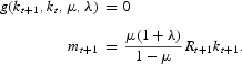
of k^D and ε>0, such that, for all μ∈(0, ε) and all k₀∈I, there exists a unique intertemporal equilibrium (k_t, m_t)_{t[ges ]0} of the economy with a liquidity constraint, with initial conditions k₀ and m₀=[μ(1+λ)]/(1−μ)R₀k₀. This equilibrium is located in I (i.e., k_t∈I∀t), and such that at each date the liquidity constraint is binding (HS regime). This trajectory converges toward a stationary equilibrium k*(μ) of the HS regime. Moreover, the sequence k_t(μ) converges uniformly toward the Diamond trajectory k_t(0) starting from k₀ when μ tends to 0.

Proof. See Appendix A.

This proposition shows that within a neighborhood of a stationary state that satisfies Assumption 2, it is possible to define an intertemporal equilibrium with money and binding liquidity constraints at each period, when μ is small enough. The trajectory of the monetary economy converges uniformly toward the nonmonetary economy as μ tends to 0. We will see, however, that this intertemporal equilibrium in the HS regime is not unique, and that other equilibria with temporary bubbles exist.

Trajectories with Bubbles

Cyclical Bubbles

We now consider a trajectory along which the economy experiences an infinite number of periods with bubbles. We are looking for cyclical equilibria where the economy experiences n periods in the T regime and p periods in the HS regime. Let us consider such a cycle of period n+p. All of the dynamics can be described by the orbit

Between periods 1 and n+1, the economy is in the T regime; between periods n+1 and (n+p)+1, the economy is in the T regime, ….

In Appendix B, we prove the following proposition.

PROPOSITION 3. Under Assumption 2, ∀n and p, such that n[ges ]1 and p[ges ]1, for μ, when it is small enough, there exists a cycle of period n+p in the neighborhood of k^D, such that the economy experiences n periods in the T regime, and p periods in the HS regime.

The proof given in Appendix B consists of writing the system of 2(n+p) equations, which defines the cyclical orbit. These equations are satisfied for μ=0 with k_i=k^D and m_i=0. Thus, the implicit function theorem makes it possible to show the existence of a solution

as a function of μ, when μ is within a neighborhood of μ=0. Finally, it is possible to prove that this solution satisfies the constraints (24) and (27).

The result is obtained for μ small enough. Michel and Wigniolle (2002) study a Cobb-Douglas example without monetary creation, which makes it possible to characterize the global dynamics of the economy. They explicitly find a decreasing relationship between the admissible period of the cycle (more precisely the admissible value of n) and the limit value for μ.

The Appropriate Policy

The utility and production functions are now respectively given by

Under the assumption of a constant money stock, Michel and Wigniolle (2002) show that this formulation makes it possible to obtain an explicit form of the global dynamics followed by the economy.

Let us assume that the rate of money creation is constant: λ_t=λ, ∀t. We introduce the new variable:

Appendix C shows that the dynamics of the economy can be summarized as HS regime between t and t+1,

T regime between t and t+1,

and for the initial condition,

In both regimes, the dynamics of (k_t, m_t) are given by

From (39), z_t must satisfy another constraint to ensure that k_t remains positive in all periods: For all t,

We assume that the economy without money (μ=0 and λ=0) is in underaccumulation:

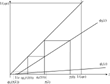
The dynamics of this economy are similar to that of Michel and Wigniolle (2003) and can be summarized as in Figure 1.

The dynamics of z.

For λ=0, we have

, because

and 1−α/[a(1−α)]<0. Thus, an equilibrium in the HS regime at all periods exists for λ=0 if (41) is satisfied:

or

An equilibrium experiencing all periods in the T regime cannot exist, because in a finite number of periods for

[condition (38)], (ϕ₀)^t(z₀) becomes negative, which is impossible.²

We assume, however, that

. Thus, the economy can experience an alternation between periods in the HS regime and periods in the T regime, and temporary bubbles may exist. Indeed, along such a trajectory, z_t shifts between the two values

. As the constraint (41) requires the inequality ϕ₀(z_t)>0 ∀t, it is possible to follow this trajectory only if

.

We wonder if a policy of monetary creation can eliminate the equilibria associated with bubbles, in ensuring the uniqueness of the equilibrium in the HS regime, such that

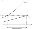
. In the figure, we show how the straight line ϕ_λ(z) and

are shifted when λ increases. If λ is high enough,

becomes negative, and the economy cannot experience any jump into the T regime. Thus, bubbles are ruled out.

Formally, it is sufficient to prove the two following points to establish this result:

• ∃λ>0 such that
  and
  . Indeed, from (35) and (41), when these two conditions hold, an equilibrium associated with a rate of money creation λ and experiencing all periods in the HS regime exists.
• . The transition from the HS regime to the T regime during one period (or more) is impossible.

The monetary policy no longer allows for a temporary bubble to exist, and ensures the uniqueness of the equilibrium. Let us show these two points.

Proof.

1. We first prove the inequality
   . We know that
   . The inequality
   is equivalent to
   
   As a(1−α)−α<0, this inequality is always satisfied for all λ>0 and μ<1.
2. We jointly consider the two inequalities
   
   Because ϕ_λ is an affine function, it is easy to calculate
   
   with
   
   Thus, the inequality
   is equivalent (after some calculations) to
   
   As by assumption α>a(1−α), for λ>0, α(1+λ)>a(1−α). Thus, for λ given, μ_t(λ) is a decreasing sequence. And for a given value of t, μ_t(λ) is a decreasing function of λ. We have to choose λ such that μ<μ₁(λ) and μ>μ₂(λ), given that μ<μ₂(0) [and μ<μ₁(0)], with
   
   
   A simple figure (Figure 2) allows us to find the appropriate values of λ, which must be in the following interval: λ₂<λ<λ₁ with
   
   with
   

The counter-bubble monetary policy.

Finally, we have shown that monetary policy makes it possible to obtain a unique equilibrium in the HS regime. Temporary bubbles can no longer exist. The monetary policy reduces the return of money, and then it becomes impossible for money to have the same return as capital. This result has been obtained under the most unfavorable circumstances: those where the created money is given to young agents. This transfer plays in favor of savings, and tends to diminish the returns on capital. We have shown that this indirect effect is dominated by the direct effect of the monetary policy.

From this result, monetary policy can be viewed as a stabilization instrument. A temporary bubble on money leads to a deflation period, where money and capital have the same return. It creates a drop in capital accumulation and production because it absorbs a share of savings. We have shown that money creation can eliminate such deflation periods because it precludes the appearance of bubbles. This result has a Keynesian flavor because it is proved that monetary creation can stabilize output fluctuations. However, this effect is not provide by demand enhancement, but by bubbles elimination.

Why Fighting Bubbles?

We have assumed in this section that the objective of the government was to fight bubbles. Indeed, bubbles reduce capital accumulation in an economy that is experiencing underaccumulation and create indetermination. Such a government's objective, however, is partly ad hoc, because it is not possible to prove that a counter-bubble policy is Pareto improving. We know that the existence of a bubble at some period is beneficial for the generation living during that period, because it increases returns on savings. It is detrimental, however, for the following generations, because it reduces capital accumulation in an economy that is experiencing underaccumulation. Thus, suppressing bubbles cannot be Pareto improving. The counter-bubble monetary policy also has a negative impact on agents' welfare because it increases the difference between the returns on the two assets—money and capital—thus increasing the distortion related to money holding.

Nevertheless, it is possible to prove that eliminating temporary bubbles can be welfare improving in a weaker sense. Let us assume that agents who meet at the beginning of time do not know when they will be alive. We can prove that there exists a large range of basic parameters (a, α, μ) such that these agents choose to eliminate bubbles, by setting a high rate of growth of the money supply.³

More precisely, we prove this property in two special cases. Indeed, when temporary bubbles may exist, there exists an infinity of equilibria that the economy can experience. Thus, we choose among these equilibria two examples of trajectories that we compare with the unique equilibrium of an economy where an appropriate policy has eliminated bubbles.

The first case is concerned with the long run of the economy. We compare the long-run properties of two economies. In the first one, bubbles are ruled out by an appropriate monetary policy, and the economy experiences a constant trajectory. In the second one, without monetary policy, it experiences a limit two-period cycle between HS and T regimes. We prove that long-run utility levels are greater in the first economy for a large range of parameters (a, α, μ). More precisely, it is possible to prove that, whatever their choice criterion is, agents at the beginning of time will prefer to eliminate bubbles for a large range of parameters because utility levels are greater during an infinite number of periods.

The second argument is more concerned with the short-run dynamics. We again compare two economies, starting from the same initial conditions. In the first one, an appropriate monetary policy has eliminated bubbles. The second one without monetary policy experiences at some date one period in the T regime. We prove that for any number of periods P, there exist parameters such that utility levels in the second economy are smaller than the minimum level in the first economy during at least P periods. Thus, under the veil of ignorance, if agents use a Rawlsian criterion between the different periods, they will prefer to live in the first economy.

The Long-Run Argument

We compare the long-run properties of two economies. In the first one, bubbles are ruled out by an appropriate monetary policy, and the economy experiences a constant trajectory. The second one, without monetary policy, experiences a limit two-period cycle between HS and T regimes.

For the first economy, the long-run value of the capital stock per young agents is given by

The second economy follows a cycle of period 2: z_t oscillates between

and

. From the preceding part, we know that such trajectory is possible under the condition

. Following (39), k_t oscillates in the long run between the two values (k₁, k₂) such that

Therefore, we obtain

It remains to prove that long-run utility levels are greater in the first economy for some range of parameters (a, α, μ). This property is proved in considering the limit case when μ→μ₂(0), with μ<μ₂(0). In this case, the value of λ allowing us to eliminate bubbles tends toward 0. And, by the definition μ₂(0), we have that

tends toward 0. Thus, we obtain

and (k₁, k₂) tends toward (0, 0). In the first economy, the long-run utility level tends to some constant value, when in the second economy it tends to −∞.⁴

This last point is easy to prove, as consumption levels (c₁, c₂, d₁, d₂) are, respectively, bounded by [f(k₁), f(k₂), (1+n)f(k₁), (1+n)f(k₂)].

In this limit case, an agent who has to choose between these two long-run states will always prefer to live in the first economy, whatever is his choice criterion. By continuity, for some choice criterion, an agent always chooses to live in the first economy for μ close to μ₂(0).

In this example, we choose for the second economy a case that can be viewed as the worst: Bubbles appears all two periods. In the following subsection, we consider the case of an economy experiencing only one period in the T regime.

The Short-Run Argument

We now consider the dynamics of two economies, starting from the same initial value of capital k₀. In the first one, bubbles are ruled out by an appropriate monetary policy λ, and we have for all t,

. From (39), k_t follows the following dynamics:

We assume that the second economy, without monetary policy, experiences all periods in the HS regime except one: Between τ and τ+1, the T regime occurs. The dynamics of k_t are

When the economy experiences a period in the T regime between τ and τ+1, the real value of money in τ+1 is higher and it absorbs a higher part of savings. Thus, there is a drop of the level of capital per young in τ+2.

As in the preceding example, we study the limit case when μ→μ₂(0), with μ<μ₂(0). In this case, the value of λ allowing bubbles to be eliminate tends toward 0, and

tends toward 0. Thus, we obtain

If we consider a given integer P, for all values of t such that

By continuity, for a given number P of periods, it is possible to find a range for the parameter μ [in a neighborhood of μ₂(0)] and a corresponding value for the monetary policy λ, such that the utility in the second economy is smaller than the minimum value of utility in the first economy during P periods. Thus, under the veil of ignorance, if agents use a Rawlsian criterion between the different periods, they will prefer to live in the first economy.