1 Introduction
The understanding of flow past a random distribution of particles has a wide range of applications. One of the major classes of application to benefit from such understanding is particle-laden multiphase flows. Particle-laden flows, where a dispersion of small particles is being carried by a continuous phase, are common in many environmental flows such as turbidity currents and volcanic eruptions, and in technological problems such as fluidized beds and slurry flows. The Eulerian–Lagrangian (EL) technique is widely used in the simulation of these particle-laden flows. In the EL technique, the location of all the particles, or a subset of computational particles that provide an accurate statistical representation of the actual distribution of particles, is tracked. The position of each particle is updated by solving the equations of motion. In the point-particle approach the flow around each particle is not resolved, and as a result, force laws are used to account for the force coupling between the particle and the continuous phase. The accuracy of the Eulerian–Lagrangian point-particle (EL-PP) technique relies heavily on the accuracy of the force laws used for the closure of the fluid–particle interaction at the microscale. These closure models must account for the net effect of the particle–flow interactions that happen at the microscale, which are unresolved in the point-particle approach.
In dilute flows, single-particle force models, such as the standard drag law that parameterizes the force coefficient in terms of the particle Reynolds number, are used to track the particle motion. With increasing particle volume fraction, the effects of the interaction of each particle with its neighbours as mediated by the continuous phase also become important and must be accounted for in the Eulerian–Lagrangian point-particle technique. The traditional approach is to modify the single-particle force models to account for the local clustering effect, by parameterizing the force coefficients in terms of both the local particle volume fraction as well as the Reynolds number. Such volume fraction-dependent drag models have been empirically obtained both by experimental measurements of the modified settling velocity of a distribution of particles (Richardson & Zaki Reference Richardson and Zaki1954) and by fully resolved simulations of flow through arrays of random particles (Beetstra, Van der Hoef & Kuipers Reference Beetstra, Van der Hoef and Kuipers2007; Tenneti, Garg & Subramaniam Reference Tenneti, Garg and Subramaniam2011; Zaidi, Tsuji & Tanaka Reference Zaidi, Tsuji and Tanaka2014; Bogner, Mohanty & Rüde Reference Bogner, Mohanty and Rüde2015; Tang et al. Reference Tang, Peters, Kuipers, Kriebitzsch and Hoef2015).
Flow past structured and random arrays of spherical particles is an important problem and has been studied in different contexts. The primary focus has been to obtain average quantities such as the mean drag on the particles, the mean velocity within the array or the mean settling velocity. One of the earliest studies in this field is by Darcy (Reference Darcy1856) who presented the first empirical model for the mean pressure drop. In the last decade, several correlations have been proposed to quantify the mean drag on particles as a function of Reynolds number and volume fraction in a monodisperse array of spherical particles (Beetstra et al. Reference Beetstra, Van der Hoef and Kuipers2007; Tenneti et al. Reference Tenneti, Garg and Subramaniam2011; Zaidi et al. Reference Zaidi, Tsuji and Tanaka2014; Bogner et al. Reference Bogner, Mohanty and Rüde2015; Tang et al. Reference Tang, Peters, Kuipers, Kriebitzsch and Hoef2015). In the two-dimensional context, bidisperse and polydisperse random arrays of cylinders have been addressed in Matsumura & Jackson (Reference Matsumura and Jackson2014a ,Reference Matsumura and Jackson b ).
Consider a random distribution of
 $N$
finite-sized particles of volume
 $V_{p}$
within a large box of volume
 $V_{B}$
. The average volume fraction of particles within the box is then
 $NV_{p}/V_{B}$
. Even when particles are randomly distributed within the box with uniform probability, there will be statistical fluctuation in any given realization. A measure of local volume fraction around each particle in a given realization can be evaluated as the number of neighbours within a reference volume element (RVE) around that particle, or the distance to the
 $m$
th nearest neighbour or using Voronoï tessellation (Monchaux, Bourgoin & Cartellier Reference Monchaux, Bourgoin and Cartellier2010, Reference Monchaux, Bourgoin and Cartellier2012) to name a few. Any such measure of local volume fraction (or equivalently local particle number density) around each particle will be a random variable that fluctuates about the mean value of
 $NV_{p}/V_{B}$
. The statistical properties of fluctuations in local particle volume fraction about the mean value can be expressed in terms of mean volume fraction (single-point statistics), radial distribution function (two-point statistics) and higher-order multi-point statistics. For a theoretical discussion on fluctuations in local particle volume fraction within a monodisperse random distribution of spheres see Stoyan & Stoyan (Reference Stoyan and Stoyan1994) and Quintanilla & Torquato (Reference Quintanilla and Torquato1997).
The random arrangement of particles within each realization in turn results in a complex microscale flow that will differ from realization to realization. Furthermore, within each realization the details of flow around each particle will be uniquely dependent on the relative position of all its neighbours. In this respect, flow around a random distribution of particles will differ from that around a regular structured array of particles of same average volume fraction. Keyser et al. (Reference Keyser, Conradie, Coertzen and Van Dyk2006) studied the effect of the particle size distribution on the flow variations and pressure drop. For a monodisperse random array of particles, significant flow and force variations within the array were observed. The fluid velocity variation in the gaps of ordered and random packs of spheres has been studied experimentally (Sederman et al. Reference Sederman, Johns, Bramley, Alexander and Gladden1997; Suekane, Yokouchi & Hirai Reference Suekane, Yokouchi and Hirai2003) and numerically (Gunjal, Ranade & Chaudhari Reference Gunjal, Ranade and Chaudhari2005). All these studies show a significant heterogeneity in the flow. Sederman et al. (Reference Sederman, Johns, Bramley, Alexander and Gladden1997) reported that 8 % of the pores carry 40 % of the volume flow. This heterogeneity in the flow reflects on the heterogeneity of the forces on each sphere.
Akiki, Jackson & Balachandar (Reference Akiki, Jackson and Balachandar2016) considered a nominally uniform flow at the macroscale over a random distribution of stationary spherical particles for varying mean particle volume fraction and varying particle Reynolds number. They showed that the drag force varies substantially from particle to particle and that the root mean square (r.m.s.) drag force fluctuation can be as high as 25 % of the mean value. This significant deviation is mainly due the fact that each individual particle within the random array sees a unique local distribution of neighbouring particles. In addition they observed the lateral force (defined as the force component in the direction normal to the mean flow) on each particle to be of comparable magnitude to the drag force. Although the mean lateral force, averaged over a large number of particles, is expected to approach zero, the r.m.s. lateral force was observed to be approximately 14 % of the mean drag force. More importantly Akiki et al. (Reference Akiki, Jackson and Balachandar2016) showed that this particle-to-particle variation in drag force cannot be correlated to local volume fraction, irrespective of which definition is used to define the local volume fraction around each particle. They were able to correlate the drag and lateral forces on the particles within the array to anisotropic measures of the exact location of the neighbouring particles. In the anisotropic measures it mattered whether the nearest neighbours are located upstream, downstream or along the lateral direction. For example, a neighbouring particle located directly upstream has a different effect on drag compared to another neighbouring particle located laterally by approximately the same distance.
These findings imply that a successful model that hopes to go beyond the mean drag force and predict the particle-to-particle variation in the drag and lateral forces must take into account the unique location of the neighbouring particles as seen by each particle within the array. In the limit of a fully resolved simulation of flow through the array, each particle knows the complete details of all the neighbours around it, and as a result, the drag force on each particle is fully informed of all the neighbours. Here we plan to pursue the following question: can the neighbourhood information around each particle, which is readily available in an EL-PP simulation from the position of the entire array of particles, be used to more accurately predict the particle-to-particle force variation, without solving for the flow details at the microscale as in a fully resolved simulation.
Langevin-type models have been proposed to account for statistical variations in the drag and lift forces on particles (Iliopoulos & Hanratty Reference Iliopoulos and Hanratty1999; Mito & Hanratty Reference Mito and Hanratty2002; Iliopoulos, Mito & Hanratty Reference Iliopoulos, Mito and Hanratty2003; Tenneti, Mehrabadi & Subramaniam Reference Tenneti, Mehrabadi and Subramaniam2016). The purpose of these models has been to account for the effect of continuous phase turbulence on particle velocity fluctuations, so that the motion of a dispersion of particles can be captured accurately in a statistical sense, even though the motion of each individual particle will not be accurate. Similar models can be used to account for the effect of fluid-mediated interaction of the neighbouring particles in the prediction of particle-to-particle force variation within a cluster. Such a model must however recognize the difference between force fluctuations due to fluid-mediated effect of neighbouring particles (pseudo-turbulence) versus that due to continuous phase turbulence. Nevertheless, such a stochastic model for force variation within a cluster can only be statistically accurate. It cannot deterministically predict increase or decrease in the particle force (above or below the mean), since it does not account for the precise arrangement of the neighbours and their influence.
There have been important advances in the experimental measurement of fluid velocity field within the gaps between the particles using non-invasive techniques like particle image velocimetry and magnetic resonance imaging (Sederman et al. Reference Sederman, Johns, Bramley, Alexander and Gladden1997). As for force measurement, Lagrangian particle tracking methods have been used where the acceleration, and correspondingly force, of each tracked individual particle can be obtained (Ayyalasomayajula et al. Reference Ayyalasomayajula, Gylfason, Collins, Bodenschatz and Warhaft2006; Qureshi et al. Reference Qureshi, Bourgoin, Baudet, Cartellier and Gagne2007; Schanz, Gesemann & Schröder Reference Schanz, Gesemann and Schröder2016).
We perform numerical experiments using direct numerical simulation (DNS) methodology, where all the particles are fully resolved, to calculate the drag and lateral forces on a distribution of spheres to a high level of accuracy. In this study, we present a simple deterministic model that attempts to predict the drag and lateral forces on each spherical particle within the array given the exact location of all the spheres, by systematically accounting for the leading-order effect of the neighbours. The accuracy of the deterministic model is then assessed by comparing its prediction against the exact forces obtained from the corresponding fully resolved DNS simulation.
We consider the zeroth-order effect of the neighbours to be the volume fraction-dependent mean drag as given in Beetstra et al. (Reference Beetstra, Van der Hoef and Kuipers2007), Tenneti et al. (Reference Tenneti, Garg and Subramaniam2011), Zaidi et al. (Reference Zaidi, Tsuji and Tanaka2014), Bogner et al. (Reference Bogner, Mohanty and Rüde2015) and Tang et al. (Reference Tang, Peters, Kuipers, Kriebitzsch and Hoef2015). So we develop a first-order correction that can account for the spatial distribution of all the particles and better predict the wide particle-to-particle variation of the drag and lift forces observed in the fully resolved DNS simulations. The development of such a model requires the following two main steps:
-
(i) We must first obtain the undisturbed flow at each particle location, where the undisturbed flow is defined as the flow that would exist at a particle location in the absence of that particle, but with all other particles present. The undisturbed flow will be obtained as a superposition of a macroscale flow that accounts for the collective action of all the particles (e.g. the mean velocity within a stationary array of particles will be higher than the superficial velocity) and microscale flow that accounts for the presence of all the neighbouring particles.
-
(ii) Using the undisturbed flow we calculate the drag and lateral forces based on the best available force model. Here we use the Faxén form of the force relation, since the undisturbed flow obtained from the first step will be strongly non-uniform due to the influence of the neighbouring particles.
The first step is achieved through a pairwise interaction approximation where the perturbation flow due to the neighbouring particles is taken into account one neighbour at a time, which are then linearly superposed to obtain the resultant undisturbed velocity. For the second step, a generalized Faxén’s form of the quasi-steady, added-mass, Basset history and vorticity-induced (lift) forces are used to obtain the total force on a particle in terms of the undisturbed velocity obtained in the first step. We will refer to this force model as the pairwise interaction extended point-particle (PIEP) model. The pairwise interactions can be pre-computed, stored as libraries and used for computing the first-order correction to the force on each particle within the array.
The ideas of accounting for the perturbation flow induced by the neighbours and using Faxén’s law are not new. In the zero Reynolds number limit, exact solutions of Stokes flow over an isolated sphere and over a pair of spheres are well known (Stimson & Jeffery Reference Stimson and Jeffery1926; Batchelor & Green Reference Batchelor and Green1972) and have been used to calculate the perturbation influence of neighbours. In the Stokes limit, the perturbation flow due to a hydrodynamic force-free particle is dominated by the stresslet, and decays as
 $1/r^{2}$
, where
 $r$
is the radial distance from the centre of the sphere. In the more general case where there is a net relative motion and hydrodynamic force, the perturbation flow includes a Stokeslet and the perturbation velocity decays very weakly as
 $1/r$
. These long range perturbations makes simultaneous interaction between multiple spheres in a multi-particle system important, whose computational resolution has led to the field of Stokesian dynamics (Brady & Bossis Reference Brady and Bossis1988). As shown by Batchelor (Reference Batchelor1972) under dilute conditions, the multi-body interaction can be limited to pairwise interactions to obtain useful results, even in the Stokes limit. The increase in volume fraction diminishes the validity of pairwise interaction assumption, but reasonable results can still be obtained even for moderate volume fractions of up to 0.2 as will be shown in this study.
The idea of superposition has been used in other contexts as well. For example in the context of collision between spherical droplets, the efficiency with which two neighbouring spheres end up colliding, as opposed to negotiating past each other without touching, depends on the perturbation flow induced by each droplet on the other. Pruppacher & Klett (Reference Pruppacher and Klett1997) introduced a simple approach based on binary superposition to account for the hydrodynamic interaction between droplet pairs. This original idea was later refined by Wang, Ayala & Grabowski (Reference Wang, Ayala and Grabowski2005) with the use of Faxén’s law, and the improved model was used in a hybrid DNS approach for simulating turbulent collisions of hydrodynamically interacting particles (Ayala, Grabowski & Wang Reference Ayala, Grabowski and Wang2007). Also of immediate relevance is the elegant force-coupling method advanced by Maxey and co-workers (Lomholt & Maxey Reference Lomholt and Maxey2003; Climent & Maxey Reference Climent, Maxey, Feuillebois and Sellier2009; Yeo & Maxey Reference Yeo and Maxey2010).
The pairwise interaction approach to be presented in this work is greatly motivated by these past efforts. However, there are significant differences. First and foremost, here we consider inertia dominated flows at particle Reynolds numbers of the order of ten to a few hundred. At such finite Reynolds numbers the perturbation flow induced by each particle decays much faster with
 $r$
, except perhaps in the wake region. This can be an advantage, since the undisturbed flow at any particle location is influenced only by its few neighbours. Furthermore, the linear additive superposition of perturbation induced by each neighbour is strictly valid in the Stokes regime, but not at finite particle Reynolds numbers. Also, the Faxén’s law, which expresses the force on a particle in terms of the surface-averaged velocity of a non-uniform undisturbed ambient flow, is rigorous only in the limit of Stokes flow. The extension and use of Faxén’s law at finite Reynolds numbers involves approximations. Finally, in Stokes flow, an average over the surface of a sphere can be rigorously expressed in terms of the velocity and its Laplacian evaluated at the centre of the sphere, since the Stokes velocity field satisfies the biharmonic equation. Such simplification is not possible at finite Reynolds numbers.
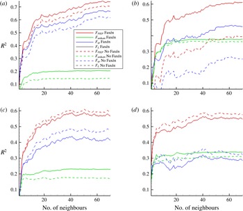
Thus, both steps of the PIEP model involve approximations and the proposed methodology can be improved. Here we have chosen the two steps to be reasonably simple so that the overall method can be implemented in an efficient manner. We emphasize that both steps of the PIEP model involve approximations and as a result the predictions of the PIEP model will not be perfect. There will be differences between the drag and lateral forces predicted from the PIEP model and those measured from the DNS. However, the results to be presented will demonstrate that the PIEP model predictions significantly better correlate with the actual force on the particles obtained from the DNS, as compared to currently best available point-particle force model.
The paper is structured as follows. In § 2, the theory for calculating the undisturbed flow and the Faxén form of the forces on each sphere in a random array are presented. The numerical methodology used in the application of the theory which leads to PIEP model is shown in § 3. In § 4, the numerical methodology used in the fully resolved DNS simulations of random arrays of spheres is presented. In § 5, we evaluate the PIEP model by comparing the drag and lateral forces obtained from PIEP model to the exact forces obtained from the fully resolved DNS simulations. Final conclusions are summarized in § 6.
2 Theory
As discussed above, in this section we will describe the two key steps of the PIEP model. In the first step we will describe a pairwise interaction model for obtaining the undisturbed flow at any given particle location that accounts for the first-order influence of all its neighbours. In the second step we will present Faxén’s form of the quasi-steady, added-mass, Basset history and vorticity-induced forces to obtain the total force on a particle in terms of the undisturbed velocity obtained in the first step.
2.1 Definition and pairwise approximation of undisturbed flow
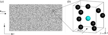
A schematic of a typical Eulerian–Lagrangian (EL) simulation is shown in figure 1. Also shown in the figure is a zoom-in of a single grid cell consisting of many particles inside. If the EL simulation employs a first-order finite volume approach, then the fluid velocity seen by all the particles shown in figure 1(b) is typically taken to be the same, and equal to the cell-centre fluid velocity. Furthermore, if the particles are stationary then the force on all the particles predicted with the standard point-particle models is the same, and there will not be any particle-to-particle force variation predicted within the cell. If the EL simulation employs a finite difference approach or a finite volume approach with second-order interpolation, then the fluid velocity at the particle location will be interpolated from the surrounding grid points or cell-centre values of fluid velocity. In this case, the fluid velocity seen by the different particles within a grid cell can vary and correspondingly there can be particle-to-particle force variation within a grid cell. However, this fluid velocity variation seen by the particles is due to continuous phase velocity variation at the sub-grid scale, which is typically small. The interpolated fluid velocity at a particle, however, does not account for the perturbation fluid velocity due to the influence of the neighbouring particles within the cell. Since the location of all the particles within the cell and their sizes are precisely known, we wish to address the following question: can the undisturbed flow seen by the
 $i$
th particle (marked blue in figure 1
b) be more accurately evaluated from the knowledge of the cell-centre (or grid point) value of the flow velocity at the macroscale and the location of all the neighbouring particles?
General schematic for EL simulations at the (a) macroscale and (b) microscale.

Consider a random distribution of spherical particles subjected to a macroscale velocity field,
 $\boldsymbol{u}_{mac}(x)$
, where
 $x$
is the spatial coordinate vector, as computed in an EL simulation. Here the macroscale velocity field has been computed at the cell centre or grid points and can be interpolated to obtain the velocity at any point
 $x$
within the computational domain. In a two-way coupled EL simulation, where the dispersed-to-continuous back coupling is accounted for, this computed macroscale velocity field
 $\boldsymbol{u}_{mac}(x)$
is, in a sense, influenced by the collective effect of all the particles.
We define
 $\boldsymbol{u}_{mic}(x_{i})$
as the microscale flow at the location
 $x_{i}$
occupied by the
 $i$
th particle due to the perturbation flow created by the presence of all other neighbouring particles. The undisturbed flow at the location of the
 $i$
th particle can then be expressed as a superposition of the macroscale flow and the microscale perturbation as,
 $$\begin{eqnarray}\displaystyle \boldsymbol{u}_{un,i}(x_{i})=\boldsymbol{u}_{mac}(x_{i})+\boldsymbol{u}_{mic,i}(x_{i}). & & \displaystyle\end{eqnarray}$$
The above separation of the undisturbed flow into a macroscale and a microscale component can be well defined in the limit where the particles are much smaller than the grid. This is the limit typically considered in the traditional point-particle approach. The Eulerian fluid velocity evaluated at the
 $i$
th particle location is the macroscale velocity,
 $\boldsymbol{u}_{mac}$
, which will be taken to be the undisturbed fluid velocity as seen by the
 $i$
th particle in the traditional point-particle approach. This macroscale velocity does not account for the sub-grid scale perturbation velocity induced by all other particles at the microscale. In (2.1)
 $\boldsymbol{u}_{mic}(x_{i})$
accounts for this microscale component of the undisturbed flow at the
 $i$
th particle. It must be pointed out that
 $\boldsymbol{u}_{mic}(x_{i})$
, thus, accounts for the pseudo-turbulence generated by the individual particles, while
 $\boldsymbol{u}_{mac}(x)$
can be a laminar flow or a turbulent flow, with flow scales only above the grid size represented.
The separation of the undisturbed flow becomes complicated, and perhaps even non-unique, when the size of the particle approaches or exceeds the grid spacing. Since the continuous phase velocity computed at the grid points is substantially influenced by the presence of such large particles, obtaining the undisturbed flow velocity becomes a challenge, even in the implementation of the point-particle approach. Recent advances by Gualtieri et al. (Reference Gualtieri, Picano, Sardina and Casciola2015), Horwitz & Mani (Reference Horwitz and Mani2016) have presented physical and numerical methodologies for the removal of self-disturbance so that the undisturbed flow velocity can be extracted. Such difficulties will persist with the application of PIEP model. Therefore, here we limit our attention to scenarios where the particles are much smaller than the grid as depicted in figure 1.
In (2.1) and henceforth we do not limit
 $x_{i}$
to be only the centre of the
 $i$
th particle, but to extend over the entire volume of the
 $i$
th particle. Thus, the undisturbed flow at the location of the
 $i$
th particle implies velocity distribution over the entire volume occupied by the particle. Even when the macroscale flow is spatially uniform, the perturbation flow due the neighbouring particles will be strongly inhomogeneous, and as a result
 $\boldsymbol{u}_{un,i}(x_{i})$
can have substantial variation over the volume occupied by the particle. This generalized definition of a spatially varying undisturbed flow is important, since later in the Faxén form of the quasi-steady and other forces, we require the undisturbed flow to be averaged over the surface or volume of the particle.
Our goal is then to find a suitable expression for the microscale component of the undisturbed velocity at the
 $i$
th particle by accounting for the relative position of all the neighbouring particles. In the limit of very dilute distribution of particles, the microscale correction
 $\boldsymbol{u}_{mic,i}(x_{i})\rightarrow 0$
and the undisturbed flow will simply approach the macroscale flow. With increasing particle volume fraction the mean inter-particle distance goes as
 $\unicode[STIX]{x1D719}^{-1/3}$
, where
 $\unicode[STIX]{x1D719}$
is the local volume fraction. So, even at modest particle volume fraction, the likelihood of finding neighbouring particles sufficiently close to contribute to the microscale component of the undisturbed flow increases.
A precise evaluation of the undisturbed flow at the location of the
 $i$
th particle,
 $\boldsymbol{u}_{un,i}(x_{i})$
, can be obtained from a fully resolved DNS simulation that includes all the other particles, except the
 $i$
th particle. But this formal definition is useful only as a conceptual picture, since the undisturbed flow at the
 $N$
particles will require
 $N$
fully resolved DNS simulations, each involving
 $N-1$
particles. Our interest is to obtain a good approximation for the undisturbed flow at the location of each of the particles, by taking into account the leading-order effect of the neighbours.
Here we propose a pairwise interaction approximation, where the perturbation flow of each of the neighbours is considered separately. The total effect of all the neighbours would then be the superposition of the individual effects. Using this pairwise interaction approximation, the undisturbed flow at the location of the
 $i$
th particle can then be simplified as,
 $$\begin{eqnarray}\displaystyle \boldsymbol{u}_{un,i}(x_{i})\approx \boldsymbol{u}_{mac}(x_{i})+\mathop{\sum }_{\substack{ j=1 \\ j\neq i}}^{N}\boldsymbol{u}_{j\rightarrow i}(x_{i}), & & \displaystyle\end{eqnarray}$$
where
 $\boldsymbol{u}_{j\rightarrow i}$
is the velocity perturbation at the
 $i$
th particle caused by the presence of the
 $j$
th particle. Here the sum is over all the
 $N$
particles except
 $j=i$
. In (2.2) the second term on the right is only an approximation to
 $\boldsymbol{u}_{mic,i}(x_{i})$
, since it accounts for the effect of the neighbouring particles one at a time and thereby ignores tertiary,
 $\boldsymbol{u}_{k\rightarrow j\rightarrow i}$
, and higher-order fluid-mediated interactions between the particles, which are implicitly captured in a fully resolved DNS.
An important advantage of the pairwise interaction approximation is that it can be implemented in an EL simulation. According to (2.2) the velocity perturbation at the
 $i$
th particle caused by the presence of the
 $j$
th particle is independent of the presence of all other particles in the neighbourhood. It depends only on the macroscale flow
 $\boldsymbol{u}_{mac}(x)$
and the relative location of the
 $i$
th particle with respect to the
 $j$
th particle. For a given macroscale flow, if we place the
 $j$
th particle at its location, it will create a perturbation flow due to its no-slip and no-penetration boundary conditions. This perturbation flow evaluated at the location of the
 $i$
th particle is
 $\boldsymbol{u}_{j\rightarrow i}(x_{i})$
. Since the definition of this perturbation flow excludes the presence of all particles except the
 $j$
th particle, this can be obtained from the flow over an isolated particle. Further, if we consider the macroscale flow to be uniform at the level of a single grid cell (as in a first-order finite volume approach),
 $\boldsymbol{u}_{j\rightarrow i}(x_{i})$
can be readily obtained from the finite Reynolds number uniform flow around an isolated particle. This evaluation of the perturbation flow from DNS of an isolated particle will be presented in § 3.
The undisturbed flow at the location of the
 $i$
th particle will be used to calculate the quasi-steady, pressure-gradient, added-mass, Basset history and vorticity-induced forces on the
 $i$
th particle. The evaluation of these forces requires not only the undisturbed velocity field at the location of the
 $i$
th particle, but also other related quantities such as the stress tensor and the vorticity of the undisturbed flow. We separate these quantities as well into a macroscale and a microscale contribution. We again employ the pairwise superposition approximation for the microscale contribution. The stress tensor of the undisturbed flow at the location of the
 $i$
th particle can be written as,
 $$\begin{eqnarray}\displaystyle -p_{un,i}(x_{i})\boldsymbol{I}+\unicode[STIX]{x1D749}_{un,i}(x_{i}) & {\approx} & \displaystyle -(p_{mac}(x_{i})+p_{mic}(x_{i}))\boldsymbol{I}+\unicode[STIX]{x1D749}_{mac}(x_{i})+\unicode[STIX]{x1D749}_{mic}(x_{i})\nonumber\\ \displaystyle & {\approx} & \displaystyle -\!\left(p_{mac}(x_{i})+\mathop{\sum }_{\substack{ j=1 \\ j\neq i}}^{N}p_{j\rightarrow i}(x_{i})\right)\boldsymbol{I}+\unicode[STIX]{x1D749}_{mac}(x_{i})+\mathop{\sum }_{\substack{ j=1 \\ j\neq i}}^{N}\unicode[STIX]{x1D749}_{j\rightarrow i}(x_{i}),\nonumber\\ \displaystyle & & \displaystyle\end{eqnarray}$$
where
 $p_{mac}$
and
 $\unicode[STIX]{x1D749}_{mac}$
are the pressure and viscous stress tensor of the macroscale flow and
 $p_{j\rightarrow i}(x_{i})$
and
 $\unicode[STIX]{x1D749}_{j\rightarrow i}(x_{i})$
are the perturbation pressure and perturbation viscous stress tensor due to the presence of the
 $j$
th particle at the location of the
 $i$
th particle, ignoring the effect of all other neighbours.
Note that the above definition involves different layers of approximation. Due to the nonlinear dependence of pressure on velocity, if we define macroscale pressure to obey the following Poisson equation:
 $\unicode[STIX]{x1D6FB}^{2}p_{mac}=-\unicode[STIX]{x1D735}\boldsymbol{\cdot }(\boldsymbol{u}_{mac}\boldsymbol{\cdot }\unicode[STIX]{x1D735}\boldsymbol{u}_{mac})$
, the corresponding Poisson equation for microscale pressure becomes
 $$\begin{eqnarray}\displaystyle \unicode[STIX]{x1D6FB}^{2}p_{mic}=-\unicode[STIX]{x1D735}\boldsymbol{\cdot }(\boldsymbol{u}_{mac}\boldsymbol{\cdot }\unicode[STIX]{x1D735}\boldsymbol{u}_{mic})-\unicode[STIX]{x1D735}\boldsymbol{\cdot }(\boldsymbol{u}_{mic}\boldsymbol{\cdot }\unicode[STIX]{x1D735}\boldsymbol{u}_{mac})-\unicode[STIX]{x1D735}\boldsymbol{\cdot }(\boldsymbol{u}_{mic}\boldsymbol{\cdot }\unicode[STIX]{x1D735}\boldsymbol{u}_{mic}) & & \displaystyle\end{eqnarray}$$
and thus
 $p_{mic}$
will depend on both micro and macroscale velocity. Here we assume
 $\boldsymbol{u}_{mac}$
to be nearly uniform on the microscale, and ignore the first two contributions on the right-hand side. In obtaining the final expression in (2.3) we assume pairwise interaction with additive contribution from each neighbour. Here again we ignore the nonlinear interaction between the different perturbations with the assumption
 $$\begin{eqnarray}\displaystyle \left(\mathop{\sum }_{\substack{ j=1 \\ j\neq i}}^{N}\boldsymbol{u}_{j\rightarrow i}\right)\boldsymbol{\cdot }\unicode[STIX]{x1D735}\left(\mathop{\sum }_{\substack{ j=1 \\ j\neq i}}^{N}\boldsymbol{u}_{j\rightarrow i}\right)\approx \mathop{\sum }_{\substack{ j=1 \\ j\neq i}}^{N}(\boldsymbol{u}_{j\rightarrow i}\boldsymbol{\cdot }\unicode[STIX]{x1D735}\boldsymbol{u}_{j\rightarrow i}). & & \displaystyle\end{eqnarray}$$
The vorticity of the undisturbed flow at the location of the
 $i$
th particle can be written as,
 $$\begin{eqnarray}\displaystyle \unicode[STIX]{x1D74E}_{un,i}(x_{i})\approx \unicode[STIX]{x1D74E}_{mac}(x_{i})+\mathop{\sum }_{\substack{ j=1 \\ j\neq i}}^{N}\unicode[STIX]{x1D74E}_{j\rightarrow i}(x_{i}), & & \displaystyle\end{eqnarray}$$
where
 $\unicode[STIX]{x1D74E}_{mac}$
is the vorticity of the macroscale flow and
 $\unicode[STIX]{x1D74E}_{j\rightarrow i}(x_{i})$
is the perturbation vorticity due to the presence of the
 $j$
th particle at the location of the
 $i$
th particle. Pairwise superposition can be employed in a similar manner to evaluate any other undisturbed flow quantity of interest at any of the particle locations, as required in the force formula to be discussed below.
2.2 Force model
Now that we have established the definition of the undisturbed flow, and an approximation to it based on pairwise interaction, in this section we will obtain an expression for the hydrodynamic force on the
 $i$
th particle. By definition the undisturbed flow
 $\boldsymbol{u}_{un,i}(x_{i})$
is the flow that would exist in the absence of the
 $i$
th particle, and the corresponding pressure and viscous stresses at the
 $i$
th particle are
 $p_{un,i}(x_{i})$
and
 $\unicode[STIX]{x1D749}_{un,i}(x_{i})$
. The presence of the
 $i$
th particle will introduce a perturbation flow, since the
 $i$
th particle’s undisturbed flow is now required to satisfy no-slip and no-penetration conditions on the
 $i$
th particle. We will term this perturbation flow self-perturbation, in order to distinguish it from the perturbation flows due to the presence of the neighbouring particles that contributed to microscale component of
 $\boldsymbol{u}_{un,i}(x_{i})$
in (2.2). Let us denote this self-perturbation flow and its pressure and viscous stress fields to be
 $\boldsymbol{u}_{i}^{\prime }(x_{i})$
,
 $p_{i}^{\prime }(x_{i})$
and
 $\unicode[STIX]{x1D749}_{i}^{\prime }(x_{i})$
. Following Maxey & Riley (Reference Maxey and Riley1983) the hydrodynamic force on the
 $i$
th particle can be expressed as
 $$\begin{eqnarray}\displaystyle \boldsymbol{F}_{i}=\oint _{S_{p}}(-p_{un,i}(x_{i})\boldsymbol{I}+\unicode[STIX]{x1D749}_{un,i}(x_{i}))\boldsymbol{\cdot }\boldsymbol{n}\,\text{d}A+\oint _{S_{p}}(-p_{i}^{\prime }(x_{i})\boldsymbol{I}+\unicode[STIX]{x1D749}_{i}^{\prime }(x_{i}))\boldsymbol{\cdot }\boldsymbol{n}\,\text{d}A, & & \displaystyle\end{eqnarray}$$
where the integrals are over the surface
 $S_{p}$
of the
 $i$
th particle. The first term on the right is the force due to the undisturbed flow and will be denoted as
 $\boldsymbol{F}_{un,i}$
, and the second term on the right is the force due to the self-perturbation flow, which will be denoted as
 $\boldsymbol{F}_{i}^{\prime }$
. Using Gauss’s theorem the surface integral can be replaced by the volume integral to obtain
 $$\begin{eqnarray}\displaystyle \boldsymbol{F}_{i}=\oint _{V_{p}}(-\unicode[STIX]{x1D735}p_{un,i}(x_{i})+\unicode[STIX]{x1D735}\boldsymbol{\cdot }\unicode[STIX]{x1D749}_{un,i}(x_{i}))\,\text{d}V+\oint _{V_{p}}(-\unicode[STIX]{x1D735}p_{i}^{\prime }(x_{i})+\unicode[STIX]{x1D735}\boldsymbol{\cdot }\unicode[STIX]{x1D749}_{i}^{\prime }(x_{i}))\,\text{d}V. & & \displaystyle\end{eqnarray}$$
In the limit when all the neighbours are far away, the boundary conditions satisfied by the self-perturbation flow are (i) on the surface of the
 $i$
th particle the self-perturbation flow should counteract the undisturbed flow to satisfy no-slip and no-penetration boundary conditions and (ii) in the far field the self-perturbation flow must decay to zero. With these requirements
 $\boldsymbol{F}_{i}^{\prime }$
is traditionally written as the sum of quasi-steady, added-mass, Basset history and vorticity-induced force contributions. Expressions for these contributions have been rigorously obtained by Gatignol (Reference Gatignol1983) and Maxey & Riley (Reference Maxey and Riley1983) in the Stokes regime, with empirical corrections that extend their applicability to finite Reynolds numbers (Magnaudet & Eames Reference Magnaudet and Eames2000; Balachandar & Eaton Reference Balachandar and Eaton2010; Crowe et al.
Reference Crowe, Schwarzkopf, Sommerfeld and Tsuji2011). It is important to note that these force expressions are based on the undisturbed flow at the location of the
 $i$
th particle, although the force
 $\boldsymbol{F}_{i}^{\prime }$
itself arises due to self-perturbation.
Here are we are interested in situations where the neighbours are close by. In which case, in addition to the boundary conditions (i) and (ii) stated above, the self-perturbation flow must also satisfy (iii) no-slip and no-penetration boundary conditions on the surface of all the neighbours. The self-perturbation flow
 $\boldsymbol{u}_{i}^{\prime }(x_{i})$
and the corresponding pressure and viscous stress fields will be affected by the presence of neighbours and therefore will deviate from what they would be for an isolated
 $i$
th particle. Thus, the neighbours play a dual role, first in perturbing the macroscale flow and defining the undisturbed flow, and second in modifying the self-perturbation flow induced by the
 $i$
th particle.
Based on the above line of reasoning, we can conceptually separate
 $\boldsymbol{F}_{i}^{\prime }$
into
 $$\begin{eqnarray}\displaystyle \boldsymbol{F}_{i}^{\prime }=\unicode[STIX]{x1D74D}_{i}^{\prime }F_{i0}^{\prime }, & & \displaystyle\end{eqnarray}$$
where
 $\boldsymbol{F}_{i0}^{\prime }$
is the force due to the self-perturbation flow, ignoring the presence of the neighbours (only in the evaluation of the self-perturbation flow) and the correction
 $\unicode[STIX]{x1D74D}_{i}^{\prime }$
accounts for the force modification due to changes in the self-perturbation flow because of the presence of neighbours. In Stokesian suspensions of finite numbers of particles, the corrections can be precisely obtained using method of reflections (Guazzelli & Morris Reference Guazzelli and Morris2011; Kim & Karrila Reference Kim and Karrila2013). Given the undisturbed flow at the
 $i$
th particle
 $\boldsymbol{F}_{i0}^{\prime }$
can be readily evaluated using the force expressions of Gatignol (Reference Gatignol1983) and Maxey & Riley (Reference Maxey and Riley1983) and their finite Reynolds number extensions. This is made possible due to the fact that
 $\boldsymbol{F}_{i0}^{\prime }$
has been defined to be force on an isolated particle. Unfortunately, Stokesian dynamics and related rigorous theoretical developments do not apply at the finite Reynolds numbers of present interest. Empirical correction functions that depend on local volume fraction must instead be used to account for the collective effect of neighbouring particles. For example, in the case of quasi-steady force,
 $\unicode[STIX]{x1D74D}_{i}^{\prime }$
would correspond to finite volume fraction correction to quasi-steady force, and so on. Such correction functions account for the presence of neighbours only in the mean sense, in terms of local volume fraction.
In summary, the force on a particle can be expressed by the following sum
 $$\begin{eqnarray}\displaystyle \boldsymbol{F}=\boldsymbol{F}_{un}+\boldsymbol{F}_{qs}+\boldsymbol{F}_{am}+\boldsymbol{F}_{bh}+\boldsymbol{F}_{L}, & & \displaystyle\end{eqnarray}$$
where we have suppressed the subscript
 $i$
. The terms on the right-hand side are respectively the undisturbed, quasi-steady, added-mass, Basset history (or viscous unsteady) and rotation-induced lift forces. All these forces can be expressed entirely in terms of the undisturbed flow characterized by
 $\boldsymbol{u}_{un,i}(x_{i})$
,
 $p_{un,i}(x_{i})$
and
 $\unicode[STIX]{x1D749}_{un,i}(x_{i})$
, without the knowledge of the precise location of the neighbours. Thus, at the present level of approximation, the PIEP model uses the precise location of the neighbouring particles only in obtaining the undisturbed flow, but the neighbours contribute to the calculation of the force due to the undisturbed flow only in an average sense. The rest of our discussion will focus attention to steady flows over an array of particles, and this allows us to further simplify the force expressions. In what follows we discuss the modelling of each of these force contributions.
2.2.1 Undisturbed flow force
The undisturbed flow force, also referred to as the pressure-gradient or the Archimedes force, is due to the pressure and viscous stress variation of the undisturbed flow over the location of the particle. Here the undisturbed flow over the
 $i$
th particle is defined as in (2.1) and thus includes the perturbation flow due to all the neighbours of the
 $i$
th particle. It is undisturbed only in the sense that it is the flow that would exist in the absence of the
 $i$
th particle. By definition, the undisturbed flow force is experienced even in the absence of the
 $i$
th particle, by the fluid volume that resides at the location of the
 $i$
th particle. From (2.8) the undisturbed flow force can be expressed as
 $$\begin{eqnarray}\displaystyle \boldsymbol{F}_{un}=V_{p}(-\unicode[STIX]{x1D735}p_{un,i}(\boldsymbol{x}_{i})+\unicode[STIX]{x1D735}\boldsymbol{\cdot }\unicode[STIX]{x1D749}_{un,i}(\boldsymbol{x}_{i})), & & \displaystyle\end{eqnarray}$$
where in evaluating the volume integral, the spatial variation of pressure-gradient and viscous stress over the volume have been ignored for now. In § 2.3 we will use Faxén’s law to systematically account for such spatial variation and obtain the more general version of the undisturbed flow force and the other force contributions to be discussed below. Separating the undisturbed flow into the macroscale and microscale contributions we obtain
 $$\begin{eqnarray}\displaystyle V_{p}(-\unicode[STIX]{x1D735}p_{mac}+\unicode[STIX]{x1D735}\boldsymbol{\cdot }\unicode[STIX]{x1D749}_{mac})+V_{p}(-\unicode[STIX]{x1D735}p_{mic,i}+\unicode[STIX]{x1D735}\boldsymbol{\cdot }\unicode[STIX]{x1D749}_{mic,i}). & & \displaystyle\end{eqnarray}$$
Finally we apply the pairwise interaction approximation (2.3) for the microscale pressure and viscous stress tensor at the
 $i$
th particle to obtain
 $$\begin{eqnarray}\displaystyle \boldsymbol{F}_{un}\approx V_{p}(-\unicode[STIX]{x1D735}p_{mac}+\unicode[STIX]{x1D735}\boldsymbol{\cdot }\unicode[STIX]{x1D749}_{mac})+V_{p}\left[-\mathop{\sum }_{\substack{ j=1 \\ j\neq i}}^{N}\unicode[STIX]{x1D735}p_{j\rightarrow i}+\mathop{\sum }_{\substack{ j=1 \\ j\neq i}}^{N}\unicode[STIX]{x1D735}\boldsymbol{\cdot }\unicode[STIX]{x1D749}_{j\rightarrow i}\right]. & & \displaystyle\end{eqnarray}$$
2.2.2 Quasi-steady force
In (2.10) all the force contributions other than
 $\boldsymbol{F}_{un}$
are due to the self-perturbation flow created by the no-slip and no-penetration boundary conditions imposed by the
 $i$
th particle. The quasi-steady force on the
 $i$
th particle can be expressed using the standard drag law (Schiller & Naumann Reference Schiller and Naumann1933) as
 $$\begin{eqnarray}\displaystyle \boldsymbol{F}_{qs}=\boldsymbol{F}_{ra}(\unicode[STIX]{x1D719},Re)+\{3\unicode[STIX]{x03C0}\unicode[STIX]{x1D707}d(\boldsymbol{u}_{un,i}(x_{i})-v_{i})[1+0.15(Re)^{0.687}]-\boldsymbol{F}_{std}\}, & & \displaystyle\end{eqnarray}$$
where
 $\boldsymbol{F}_{ra}(\unicode[STIX]{x1D719},Re)$
is a suitable expression for the mean drag as a function of mean Reynolds number and mean volume fraction. In the above
 $v_{i}$
is the velocity of the
 $i$
th particle and the Reynolds number of the
 $i$
th particle is defined as,
 $$\begin{eqnarray}\displaystyle Re=\frac{d|\boldsymbol{u}_{mac}(\boldsymbol{x}_{i})-v_{i}|}{\unicode[STIX]{x1D708}}, & & \displaystyle\end{eqnarray}$$
with
 $\unicode[STIX]{x1D708}$
being the viscosity of the fluid and
 $d$
the particle diameter. In the above
 $\boldsymbol{F}_{std}$
is the standard drag on the
 $i$
th particle ignoring the influence of the neighbours at the microscale. It then depends only the macroscale flow and is given by
 $$\begin{eqnarray}\displaystyle \boldsymbol{F}_{std}=3\unicode[STIX]{x03C0}\unicode[STIX]{x1D707}d(\boldsymbol{u}_{mac}(x_{i})-v_{i})[1+0.15(Re)^{0.687}]. & & \displaystyle\end{eqnarray}$$
Thus, the second term in (2.14) within the curly parenthesis accounts for the quasi-steady effect of the perturbation flow created by the neighbouring particles at the microscale (i.e. quasi-steady force due to
 $\boldsymbol{u}_{un,i}(x_{i})-\boldsymbol{u}_{mac}(x_{i})$
). It should be noted that the standard drag law by Schiller and Naumann is valid for up to
 $Re_{p}\approx 1000$
. Any other finite Reynolds number drag law (Clift, Grace & Weber Reference Clift, Grace and Weber1978; Khan & Richardson Reference Khan and Richardson1987; Brown & Lawler Reference Brown and Lawler2003) can be used instead in (2.14).
The standard drag correlation used in both terms within the curly parenthesis of (2.14) is for an isolated particle. It has now been well established that mean drag force on a particle within a random bed of particles is substantially higher than what will be predicted by the standard drag relation (Hill, Koch & Ladd Reference Hill, Koch and Ladd2001; Tenneti et al.
Reference Tenneti, Garg and Subramaniam2011). The increase in quasi-steady mean drag is due to the fact that the self-perturbation flow around a particle, even under steady conditions, is strongly influenced by the presence of other particles, and differs from that of an isolated particle. The average influence of finite volume fraction has been incorporated into enhanced drag law relations which are dependent on both the macroscale Reynolds number
 $(Re)$
and the macroscale volume fraction
 $(\unicode[STIX]{x1D719})$
. A few such drag laws, denoted as
 $\boldsymbol{F}_{ra}(\unicode[STIX]{x1D719},Re)$
, obtained from the literature (Beetstra et al.
Reference Beetstra, Van der Hoef and Kuipers2007; Tenneti et al.
Reference Tenneti, Garg and Subramaniam2011; Zaidi et al.
Reference Zaidi, Tsuji and Tanaka2014; Bogner et al.
Reference Bogner, Mohanty and Rüde2015; Tang et al.
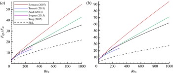
Reference Tang, Peters, Kuipers, Kriebitzsch and Hoef2015) are plotted alongside (2.16) in figure 2 for volume fractions of 0.1 and 0.21. (The subscript ‘ra’ denotes the mean drag correlation for a random distribution of particles. The results for structured arrays of particles, such as body-centred cubic or face-centred cubic arrangements, will have different mean drag correlation.) Although there is significant difference between the different finite volume fraction drag laws, all the correlations suggest a higher drag than the standard drag law due to the intrinsic effects within the array, which are amplified with increasing volume fraction. In the results to be presented we will use the mean drag correlation by Tenneti et al. (Reference Tenneti, Garg and Subramaniam2011) for
 $\boldsymbol{F}_{ra}(\unicode[STIX]{x1D719},Re)$
but qualitatively similar results are obtained with the use of other finite volume fraction drag laws.
Drag laws for finite volume fractions versus the superficial Reynolds number for (a)
 $\unicode[STIX]{x1D719}=0.1$
and (b)
 $\unicode[STIX]{x1D719}=0.21$
. The standard drag law (SDL) for a single sphere is plotted alongside for comparison.

The quasi-steady drag relation (2.14) can now be interpreted in the following way. Given the macroscale information (i.e. local volume fraction at the macroscale, Reynolds number based on the macroscale flow) the best estimate of the mean quasi-steady drag is given by
 $\boldsymbol{F}_{ra}(\unicode[STIX]{x1D719},Re)$
. The purpose of the second term is to account for the perturbation to the quasi-steady force due to changes in the undisturbed flow at the location of the
 $i$
th particle induced by the local arrangement of neighbouring particles. When (2.2) and (2.16) are substituted for
 $\boldsymbol{u}_{un,i}$
and
 $\boldsymbol{F}_{std}$
, the second term within the curly parenthesis in (2.14) becomes,
 $$\begin{eqnarray}\displaystyle 3\unicode[STIX]{x03C0}\unicode[STIX]{x1D707}d\left(\mathop{\sum }_{\substack{ j=1 \\ j\neq i}}^{N}\boldsymbol{u}_{j\rightarrow i}(x_{i})\right)[1+0.15(Re)^{0.687}]. & & \displaystyle\end{eqnarray}$$
The above perturbation force will approach zero when averaged over a large number of particles and over an ensemble of realizations. From the definition of perturbation velocity we expect
 $$\begin{eqnarray}\displaystyle \left\langle \mathop{\sum }_{\substack{ j=1 \\ j\neq i}}^{N}\boldsymbol{u}_{j\rightarrow i}(x_{i})\right\rangle \rightarrow 0, & & \displaystyle\end{eqnarray}$$
where the angle brackets represent an average over an ensemble of realizations. This will ensure that the mean drag force for a steady macroscale flow will correctly reduce to
 $\boldsymbol{F}_{ra}(\unicode[STIX]{x1D719},Re)$
.
Finally, the expression (2.14) for the quasi-steady force is not the only acceptable form. For example, the definition of the Reynolds number of the
 $i$
th particle can be based on undisturbed fluid velocity, as opposed to the macroscale velocity. In other words,
 $Re_{i}$
in (2.14) can be replaced by
 $d|\boldsymbol{u}_{un,i}(\boldsymbol{x}_{i})-v_{i}|/\unicode[STIX]{x1D708}$
. With this modification, however, it is not clear if the perturbation force within the curly parenthesis on the right-hand side of (2.14) summed over an ensemble of realizations will reduce to zero.
2.2.3 Added-mass force
The added-mass force arises from the relative acceleration of the undisturbed flow at the particle location with respect to the acceleration of the particle. This force is expressed as
 $$\begin{eqnarray}\displaystyle \boldsymbol{F}_{am} & = & \displaystyle C_{m}m_{f}\left(\frac{\text{D}\boldsymbol{u}_{un,i}(x_{i})}{\text{D}t}-\frac{\text{d}v_{i}}{\text{d}t}\right)\nonumber\\ \displaystyle & = & \displaystyle C_{m}m_{f}\left(\frac{\text{D}\boldsymbol{u}_{mac}(x_{i})}{\text{D}t}-\frac{\text{d}v_{i}}{\text{d}t}\right)+C_{m}V_{p}(-\unicode[STIX]{x1D735}p_{mic,i}(x_{i})+\unicode[STIX]{x1D735}\boldsymbol{\cdot }\unicode[STIX]{x1D749}_{mic,i}(x_{i}))\nonumber\\ \displaystyle & {\approx} & \displaystyle C_{m}m_{f}\left[\frac{\text{D}\boldsymbol{u}_{mac}(x_{i})}{\text{D}t}-\frac{\text{d}v_{i}}{\text{d}t}\right]+C_{m}V_{p}\left[-\mathop{\sum }_{\substack{ j=1 \\ j\neq i}}^{N}\unicode[STIX]{x1D735}p_{j\rightarrow i}(x_{i})+\mathop{\sum }_{\substack{ j=1 \\ j\neq i}}^{N}\unicode[STIX]{x1D735}\boldsymbol{\cdot }\unicode[STIX]{x1D749}_{j\rightarrow i}(x_{i})\right].\nonumber\\ \displaystyle & & \displaystyle\end{eqnarray}$$
Note that both the flow acceleration as well as the acceleration of the
 $i$
th particle contribute to the added-mass force. Again, the flow acceleration has been separated into macroscale and microscale contributions. We have used the pairwise interaction approximation (2.2) to simplify the microscale contribution. In the present problem of a steady flow over a stationary bed of particles,
 $\text{d}v_{i}/\text{d}t=0$
and
 $\unicode[STIX]{x2202}\boldsymbol{u}_{un,i}/\unicode[STIX]{x2202}t=0$
. But the total acceleration of the undisturbed flow at the location of the
 $i$
th particle may not be zero due to convective acceleration (i.e.
 $\text{D}\boldsymbol{u}_{un,i}(x_{i})/\text{D}t$
is equal to
 $\unicode[STIX]{x2202}\boldsymbol{u}_{un,i}(x_{i})\boldsymbol{\cdot }\unicode[STIX]{x1D735}\boldsymbol{u}_{un,i}(x_{i})$
which may be non-zero). Thus,
 $\boldsymbol{F}_{am}$
can be non-zero even in a steady flow through an array of particles. This force arises from the self-perturbation flow that results from the imposition of no-penetration boundary condition on the surface of the
 $i$
th particle. In the above equation
 $C_{m}$
is the added-mass coefficient and is equal to
 $1/2$
for an isolated sphere. The added-mass coefficient has been shown to increase with particle volume fraction. Zuber (Reference Zuber1964) and Sangani, Zhang & Prosperetti (Reference Sangani, Zhang and Prosperetti1991) have shown the added-mass coefficient to scale as
 $(1+2\unicode[STIX]{x1D719}_{mac})/2$
for small values of volume fraction.
2.2.4 Basset history force
The Basset history force arises from the viscous effect of relative acceleration of the undisturbed flow at the particle location with respect to the acceleration of the particle. This force is also known as the viscous unsteady force and it can be expressed as a convolution integral (Maxey & Riley Reference Maxey and Riley1983; Magnaudet & Eames Reference Magnaudet and Eames2000; Balachandar & Eaton Reference Balachandar and Eaton2010)
 $$\begin{eqnarray}\displaystyle \boldsymbol{F}_{bh}=\frac{3}{2}d^{2}\sqrt{\unicode[STIX]{x03C0}\unicode[STIX]{x1D70C}\unicode[STIX]{x1D707}}\int _{-\infty }^{t}K_{bh}(t-\unicode[STIX]{x1D70F})\left(\frac{\text{d}\boldsymbol{u}_{un,i}}{\text{d}t}-\frac{\text{d}v_{i}}{\text{d}t}\right)_{@\unicode[STIX]{x1D70F}}\,\text{d}\unicode[STIX]{x1D70F}, & & \displaystyle\end{eqnarray}$$
where
 $\unicode[STIX]{x1D70C}$
and
 $\unicode[STIX]{x1D707}$
are the density and viscosity of the fluid, respectively, and the subscript
 $@\unicode[STIX]{x1D70F}$
indicates that the relative acceleration is evaluated at time equal to
 $\unicode[STIX]{x1D70F}$
. The Basset history kernel
 $K_{bh}$
has a
 $1/\sqrt{(t-\unicode[STIX]{x1D70F})}$
behaviour for small values of the argument, but for larger values of the argument the kernel decays more rapidly as
 $1/(t-\unicode[STIX]{x1D70F})^{2}$
or faster (Mei & Adrian Reference Mei and Adrian1992; Lovalenti & Brady Reference Lovalenti and Brady1993; Kim, Elghobashi & Sirignano Reference Kim, Elghobashi and Sirignano1998). Unfortunately, the precise form of the kernel somewhat depends on the nature of the problem. Nevertheless in the present problem, according to the definition given above, the Basset history force is identically zero for all the particles. This is because
 $\text{d}\boldsymbol{u}_{un,i}/\text{d}t$
is the total derivative of the undisturbed flow at the
 $i$
th particle following the particle, which is identically zero since we consider a steady flow over a stationary distribution of particles.
Here we have followed Maxey & Riley (Reference Maxey and Riley1983) and Balachandar & Eaton (Reference Balachandar and Eaton2010) and defined fluid acceleration to be different in the added-mass and Basset history forces (i.e.
 $\text{D}\boldsymbol{u}_{un,i}/\text{D}t$
in added mass versus
 $\text{d}\boldsymbol{u}_{un,i}/\text{d}t$
in Basset history force). As pointed out by Maxey & Riley (Reference Maxey and Riley1983) their difference can be ignored in the linear limit, but not in the finite Reynolds number regime. Solution of the linearized Navier–Stokes equations for the unsteady Stokes flow over an arbitrarily moving particle by Gatignol (Reference Gatignol1983) and Maxey & Riley (Reference Maxey and Riley1983) yielded
 $\text{d}\boldsymbol{u}_{un,i}/\text{d}t$
for both the unsteady forces. Based on the inviscid analysis of Auton (Reference Auton1987) and Auton, Hunt & Prud’Homme (Reference Auton, Hunt and Prud’Homme1988) the added-mass force in (2.19) is written in terms of
 $\text{D}\boldsymbol{u}_{un,i}/\text{D}t$
. For now, we will consider the Basset history force to be zero in the present steady flow, but later in the discussion section we will consider the effect of alternate forms of the Basset history force.
2.2.5 Rotational force
Even when the ambient flow at the macroscale
 $\boldsymbol{u}_{mac}$
is irrotational, the
 $i$
th particle will be subjected to a vortical flow, since it is immersed in the perturbation flow of the neighbouring particles. A simple example is the
 $i$
th particle sitting in the vortical wake of an upstream neighbour. The hydrodynamic force on a particle due to ambient vorticity can be separated into an inviscid contribution and a viscous contribution. A simple model of the rotational force is
 $$\begin{eqnarray}\displaystyle F_{L}\approx C_{L}m_{f}[(\boldsymbol{u}_{un,i}(\boldsymbol{x}_{i})-v_{i})\times (\unicode[STIX]{x1D714}_{un,i}(\boldsymbol{x}_{i})+2\unicode[STIX]{x1D734}_{i})], & & \displaystyle\end{eqnarray}$$
where
 $\unicode[STIX]{x1D734}_{i}$
is the angular velocity of the particle and
 $C_{L}$
is the lift coefficient. In the above equation the undisturbed flow velocity and vorticity can be approximated with the pairwise interaction model given in (2.2) and (2.6). From the analysis of Auton et al. (Reference Auton, Hunt and Prud’Homme1988)
 $C_{L}$
is
 $1/2$
for an isolated stationary sphere in a steady weak ambient vorticity field. In the more general case of a translating and rotating sphere in an ambient vortical field, the effects of ambient vorticity and particle rotation superpose, and alternate expressions for the lift coefficient have been proposed (Rubinow & Keller Reference Rubinow and Keller1961; Saffman Reference Saffman1965). The effects of finite Reynolds number, finite volume fraction, or time dependence further complicates the rotational or lift force model (Bagchi & Balachandar Reference Bagchi and Balachandar2002a
,Reference Bagchi and Balachandar
b
; Wakaba & Balachandar Reference Wakaba and Balachandar2005). Here we have chosen to use the simple expression (2.21) with
 $C_{L}=1/2$
to model the rotational force. As we will see in the results section, the rotational force does not make a significant contribution to the overall force model.
2.3 Faxén form of the forces
The undisturbed flow at the
 $i$
th particle
 $\boldsymbol{u}_{un,i}(x_{i})$
can be expected to substantially vary on the scale of the
 $i$
th particle. However, the different force contributions given in (2.13), (2.14), (2.19) and (2.21) implicitly assume the undisturbed flow quantities, such as
 $\boldsymbol{u}_{un,i}(x_{i})$
,
 $p_{un,i}(x_{i})$
,
 $\unicode[STIX]{x1D749}_{un,i}(x_{i})$
and
 $\unicode[STIX]{x1D74E}_{un,i}(x_{i})$
, to be defined at the centre of the
 $i$
th particle. For the present non-uniform undisturbed flow we will consider the generalization of the Faxén’s theorem (Reference Faxén1922) by Gatignol (Reference Gatignol1983) and Maxey & Riley (Reference Maxey and Riley1983). For a spatially varying ambient flow the undisturbed flow force can be generalized as
 $$\begin{eqnarray}\displaystyle \boldsymbol{F}_{un}=V_{p}(-\overline{\unicode[STIX]{x1D735}p_{mac}}^{V}+\overline{\unicode[STIX]{x1D735}\boldsymbol{\cdot }\unicode[STIX]{x1D749}_{mac}}^{V})+V_{p}\left(\mathop{\sum }_{\substack{ j=1 \\ j\neq i}}^{N}[-\overline{\unicode[STIX]{x1D735}p_{j\rightarrow i}}^{V}+\overline{\unicode[STIX]{x1D735}\boldsymbol{\cdot }\unicode[STIX]{x1D749}_{j\rightarrow i}}^{V}]\right), & & \displaystyle\end{eqnarray}$$
where
 $\overline{()}^{V}$
indicates an average over the volume of the
 $i$
th particle. By Gauss’s theorem,
 $\boldsymbol{F}_{un}$
correctly reduces to the integral of the undisturbed pressure and viscous stresses over the surface of the particle. In obtaining the last equation we have commuted the summation operation over the neighbours and the volume integral. In the final form, the undisturbed flow force due to the macroscale flow and that due to the perturbation of each neighbouring particle has been separated.
The Faxén form of the quasi steady force can be expressed as
 $$\begin{eqnarray}\displaystyle \boldsymbol{F}_{qs}=\boldsymbol{F}_{ra}(\unicode[STIX]{x1D719},Re)+\left\{3\unicode[STIX]{x03C0}\unicode[STIX]{x1D707}d\left(\mathop{\sum }_{\substack{ j=1 \\ j\neq i}}^{N}\overline{\boldsymbol{u}_{j\rightarrow i}(x_{i})}^{S}\right)[1+0.15(Re)^{0.687}]\right\}, & & \displaystyle\end{eqnarray}$$
where
 $\overline{()}^{S}$
indicates an average over the surface of the
 $i$
th particle and
 $S_{p}=4\unicode[STIX]{x03C0}R^{2}$
is the surface area of the
 $i$
th particle. Following the derivation of the undisturbed fluid force presented above, the Faxén form of the added-mass force can be expressed as
 $$\begin{eqnarray}\displaystyle \boldsymbol{F}_{am}=C_{m}m_{f}\left[\frac{\overline{\text{D}\boldsymbol{u}_{mac}(x_{i})}^{V}}{\text{D}t}-\frac{\text{d}\boldsymbol{v}_{i}}{\text{d}t}\right]+C_{m}V_{p}\left(\mathop{\sum }_{\substack{ j=1 \\ j\neq i}}^{N}[-\overline{\unicode[STIX]{x1D735}p_{j\rightarrow i}}^{V}+\overline{\unicode[STIX]{x1D735}\boldsymbol{\cdot }\unicode[STIX]{x1D749}_{j\rightarrow i}}^{V}]\right), & & \displaystyle\end{eqnarray}$$
where we have used the fact that the translational acceleration of the particle remains the same over the entire particle.
Finally, due to its nonlinear dependence on velocity, the rotational force can be extended in several different ways in the case of spatially varying undisturbed flow. The form that has been used in the results to be presented below is
 $$\begin{eqnarray}\displaystyle \boldsymbol{F}_{L}\approx C_{ir}m_{f}\left[\overline{\boldsymbol{u}_{mac}(x_{i})}^{V}+\mathop{\sum }_{\substack{ j=1 \\ j\neq i}}^{N}\overline{\boldsymbol{u}_{j\rightarrow i}(x_{i})}^{V}-v_{i}\right]\times \left[\overline{\unicode[STIX]{x1D74E}_{mac}(x_{i})}^{V}+\mathop{\sum }_{\substack{ j=1 \\ j\neq i}}^{N}\overline{\unicode[STIX]{x1D714}_{j\rightarrow i}(x_{i})}^{V}+2\unicode[STIX]{x1D734}_{i}\right]. & & \displaystyle \nonumber\\ \displaystyle & & \displaystyle\end{eqnarray}$$
Note that in the above definition (i) we first average velocity and vorticity perturbations over the volume of the
 $i$
th particle, (ii) the volume averages are then summed over all the neighbours and added to the corresponding macroscale contribution and (iii) finally the cross-product of the net velocity and vorticity contribute to the rotational force. But the order of these operations can be rearranged to get a different definition of the rotational force. Also the above definition using volume averages is somewhat arbitrary. Instead, the volume averages can be replaced by averages over the surface of the
 $i$
th particle. Unfortunately, the rigorous theory of Gatignol (Reference Gatignol1983) and Maxey & Riley (Reference Maxey and Riley1983) is based on linear approximation and does not provide the precise form of the nonlinear rotational force. We have tried different forms of the inviscid rotational force, and since the contribution of
 $\boldsymbol{F}_{L}$
is generally small, the results to be presented are not sensitive to the precise form.
In summary, the PIEP model force is given by,
 $$\begin{eqnarray}\displaystyle \boldsymbol{F}=\boldsymbol{F}_{un}+\boldsymbol{F}_{qs}+\boldsymbol{F}_{am}+\boldsymbol{F}_{L}, & & \displaystyle\end{eqnarray}$$
where the four force contributions on the right-hand side are given by (2.22), (2.23), (2.24) and (2.25), respectively.
3 DNS of an isolated sphere
As defined by the pairwise interaction approximation given in (2.2), (2.3) or (2.6), the undisturbed flow is expressed as a summation of the macroscale flow and a superposition of the perturbation flows generated by the neighbouring particles, taken one at a time. In particular, we assume the perturbation at the
 $i$
th particle due to the
 $j$
th particle to be independent of the presence of all other particles in the neighbourhood. In order to calculate this perturbation due to the
 $j$
th particle (which is denoted as
 $\boldsymbol{u}_{j\rightarrow i}(x_{i})$
in (2.2)), we only need to know (i) the macroscale flow and (ii) the relative position of the
 $i$
th particle with respect to the
 $j$
th particle. By definition, the undisturbed flow at the
 $i$
th particle is a flow that would exist in the absence of the
 $i$
th particle. As per pairwise interaction approximation, the contribution to the undisturbed flow from the
 $j$
th neighbour excludes the presence of all other neighbours. Thus, the surface and volume averages in the Faxén form of the force contributions (i.e.
 $\overline{\boldsymbol{u}_{j\rightarrow i}(x_{i})}^{S}$
,
 $\overline{\boldsymbol{u}_{j\rightarrow i}(x_{i})}^{V}$
,
 $\overline{\unicode[STIX]{x1D735}p_{j\rightarrow i}}^{V}$
,
 $\overline{\unicode[STIX]{x1D735}\boldsymbol{\cdot }\unicode[STIX]{x1D749}_{j\rightarrow i}}^{V}$
,
 $\overline{\unicode[STIX]{x1D714}_{j\rightarrow i}(x_{i})}^{V}$
) can be obtained from flow over an isolated particle. Further, here we consider the macroscale flow to be uniform and thus the particle Reynolds number based on the macroscale velocity
 $(Re_{i})$
is the only parameter.
3.1 Numerical methodology
An isolated sphere in a uniform ambient flow presents a relatively simple geometry. At Reynolds numbers below 200 the flow remains steady and axisymmetric, thus allowing highly resolved simulations with a two-dimensional polar grid fitted around the sphere. Here we use a fully spectral simulation with Fourier representation in the circumferential direction and Chebyshev representation along the radial direction (Bagchi & Balachandar Reference Bagchi and Balachandar2002a ,Reference Bagchi and Balachandar b ). The computational domain is chosen to be a larger sphere of radius 15 diameters, which has been shown to be sufficiently large in prior investigations of flow over a sphere. A Chebyshev–Gauss–Lobatto distribution of grid points is used in the radial direction, starting from the definition
 $$\begin{eqnarray}\displaystyle \unicode[STIX]{x1D709}_{i}=-\cos \left(\frac{\unicode[STIX]{x03C0}(i-1)}{N_{r}-1}\right), & & \displaystyle\end{eqnarray}$$
where
 $N_{r}$
is the number of grid points in the radial direction. A transformation is then implemented to stretch the grid and allocate more points in the region close to the sphere where velocity gradients are more prominent. The transformation is given by,
 $$\begin{eqnarray}\displaystyle \hat{\unicode[STIX]{x1D709}}_{i}=C_{0}+C_{1}\unicode[STIX]{x1D709}_{i}-C_{0}\unicode[STIX]{x1D709}_{i}^{2}+C_{3}\unicode[STIX]{x1D709}_{i}^{3}. & & \displaystyle\end{eqnarray}$$
By requiring
 $\hat{\unicode[STIX]{x1D709}}(\unicode[STIX]{x1D709}=1)=1$
and
 $\hat{\unicode[STIX]{x1D709}}(\unicode[STIX]{x1D709}=-1)=-1$
, we constrain the constants
 $C_{1}$
and
 $C_{3}$
to,
 $$\begin{eqnarray}\displaystyle \left.\begin{array}{@{}c@{}}\displaystyle C_{1}=0.5(-\unicode[STIX]{x1D6FE}_{1}+2C_{0}+3),\\ \displaystyle C_{3}=0.5(\unicode[STIX]{x1D6FE}_{1}-2C_{0}-1).\end{array}\right\} & & \displaystyle\end{eqnarray}$$
The extent of the stretch is thus determined by the constants
 $C_{0}$
and
 $\unicode[STIX]{x1D6FE}_{1}$
, which are chosen to be 0.6 and 0.2 in the present simulations. The grid points in the radial direction are then scaled to cover the whole domain from the radius of the particle
 $(r_{in})$
to the radius of the outer spherical domain
 $(r_{out})$
,
 $$\begin{eqnarray}\displaystyle r_{i}={\textstyle \frac{1}{2}}\hat{\unicode[STIX]{x1D709}}_{i}[r_{in}-r_{out}]+{\textstyle \frac{1}{2}}[r_{in}+r_{out}],\quad \text{for }i=1,2,\ldots ,N_{r}. & & \displaystyle\end{eqnarray}$$
By symmetry the grid points in the tangential direction are defined from 0 to
 $\unicode[STIX]{x03C0}$
. Here again the grid points are stretched and clustered in the wake region to provide increased resolution of the wake vortical structures:
 $$\begin{eqnarray}\displaystyle \unicode[STIX]{x1D703}(j)=\tan ^{-1}\left(\frac{\sin \displaystyle \left(\frac{\unicode[STIX]{x03C0}}{N_{\unicode[STIX]{x1D703}}}(j-1/2)\right)(1-h^{2})}{\cos \displaystyle \left(\frac{\unicode[STIX]{x03C0}}{N_{\unicode[STIX]{x1D703}}}(j-1/2)\right)(1+h^{2})-2h}\right),\quad \text{for }j=1,2,\ldots ,N_{\unicode[STIX]{x1D703}}, & & \displaystyle\end{eqnarray}$$
where
 $N_{\unicode[STIX]{x1D703}}$
is the number of grid points in the tangential direction. The grid is stretched towards the downstream direction by specifying a negative parameter
 $h$
. In the present simulations
 $h$
is set to
 $-0.35$
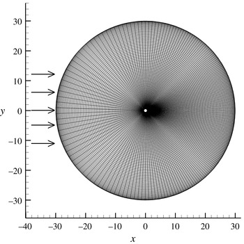
which provides a higher resolution in the wake of the sphere. A schematic of the grid is shown in figure 3.
Body fitted spherical mesh used for the single-particle simulations.
 $N_{r}=121$
,
 $N_{\unicode[STIX]{x1D703}}=100$
,
 $C_{0}=0.6$
,
 $\unicode[STIX]{x1D6FE}_{1}=0.2$
and
 $h=-0.35$
. The arrows indicate the direction of the flow.

A Dirichlet boundary condition for a uniform flow of unit non-dimensional magnitude is imposed at the inlet. A non-reflecting boundary condition is used at the outflow by parabolizing the governing equations (Mittal & Balachandar Reference Mittal and Balachandar1996). The Fourier–Chebyshev spectral method is used to solve the governing equations given by the non-dimensional incompressible Navier–Stokes equations,
 $$\begin{eqnarray}\displaystyle & \displaystyle \unicode[STIX]{x1D735}\boldsymbol{\cdot }\boldsymbol{u}=0, & \displaystyle\end{eqnarray}$$
 $$\begin{eqnarray}\displaystyle & \displaystyle \frac{\unicode[STIX]{x2202}\boldsymbol{u}}{\unicode[STIX]{x2202}t}+\boldsymbol{u}\boldsymbol{\cdot }\unicode[STIX]{x1D735}\boldsymbol{u}=\unicode[STIX]{x1D735}p+\frac{1}{Re}\unicode[STIX]{x1D6FB}^{2}\boldsymbol{u}. & \displaystyle\end{eqnarray}$$
A mixed second-order Adams–Bashforth and Crank–Nicolson scheme is used for the time discretization. A resolution of
 $N_{r}=121$
and
 $N_{\unicode[STIX]{x1D703}}=100$
is used. A more detailed description on the numerical scheme can be found in Bagchi & Balachandar (Reference Bagchi and Balachandar2002a
). In the above equations all the variables are non-dimensional, with the particle diameter as the length scale and the uniform inflow velocity as the velocity scale. Correspondingly, pressure is scaled by density times the square of uniform inflow velocity. Henceforth we will consider only non-dimensional quantities (unless explicitly stated otherwise).
3.2 Pairwise interaction force maps
Using the above described Fourier–Chebyshev spectral method, flow around an isolated sphere was simulated for a range of Reynolds numbers from 10 to 215. A sample result for
 $Re=87$
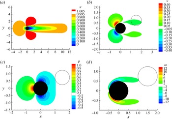
is shown in figure 4, where frames (a–d) present contour plots of streamwise
 $(x)$
velocity, cross-stream
 $(y)$
velocity, pressure and circumferential vorticity. Note that the mean value of non-dimensional streamwise velocity is unity, while the mean value of all other quantities are zero. The macroscale flow being considered is
 $\boldsymbol{u}_{mac}=1$
and
 $\unicode[STIX]{x1D74E}_{mac}=0$
. The steady velocity fields, pressure and vorticity shown in figure 4 represent well known results. Here they have been obtained at high resolution, so that they can be used in the pairwise interaction model.
Contour plots of the (a) streamwise velocity, (b) spanwise velocity, (c) pressure and (d) vorticity obtained for a uniform ambient flow over a sphere (shaded black) at
 $Re_{i}=87$
. The plots are on the
 $x$
–
 $y$
plane passing through the centre of the sphere. These results are used in the evaluation of the perturbation flow. The black shaded sphere is the
 $j$
th neighbouring sphere (source of the perturbation) while the open circle represents the
 $i$
th sphere, where the effect of the perturbation will be evaluated. The open circle represents a virtual sphere which does not affect the contour plots shown.

The central sphere in figure 4 represents the
 $j$
th particle and the quantities plotted are the perturbation flow due to the presence of the
 $j$
th particle in the uniform macroscale flow. As an example, now consider a particular location of the
 $i$
th particle as represented by the thin black circle in figure 4. With respect to the centre of this
 $i$
th particle the
 $j$
th particle is 1.5 non-dimensional units upstream and 0.75 units shifted down along the
 $y$
axis. The volume and surface integrals of the various perturbation quantities defined in the Faxén form of the force expressions (2.22)–(2.25) can now be evaluated. For the specific location of the
 $i$
th particle with respect to the
 $j$
th particle shown in figure 4 we obtain
 $$\begin{eqnarray}\displaystyle \left.\begin{array}{@{}c@{}}\displaystyle \overline{\boldsymbol{u}_{j\rightarrow i}}^{S}=-0.19\boldsymbol{e}_{x}-0.04\boldsymbol{e}_{y},\quad \overline{\boldsymbol{u}_{j\rightarrow i}}^{V}=-0.18\boldsymbol{e}_{x}-0.05\boldsymbol{e}_{y},\\ \displaystyle \overline{\unicode[STIX]{x1D735}p_{j\rightarrow i}}^{V}=-0.04\boldsymbol{e}_{x}-(1.9\times 10^{-3})\boldsymbol{e}_{y},\\ \displaystyle \overline{\unicode[STIX]{x1D735}\boldsymbol{\cdot }\unicode[STIX]{x1D749}_{j\rightarrow i}}^{V}=-0.002\boldsymbol{e}_{x}+0.0027\boldsymbol{e}_{y},\quad \overline{\unicode[STIX]{x1D74E}_{j\rightarrow i}}^{V}=-0.74\boldsymbol{e}_{z}.\end{array}\right\} & & \displaystyle\end{eqnarray}$$
The position of the
 $i$
th particle with respect to the
 $j$
th particle is systematically varied and the requisite volume or surface integrals are computed from the single-particle DNS perturbation field. The contours of the resulting streamwise
 $(x)$
and lateral
 $(y)$
components of surface-averaged velocity
 $\overline{\boldsymbol{u}_{j\rightarrow i}}^{S}$
are shown in figure 5. The surface average can be considered as a filter operation and therefore the contour plots in figure 5 are similar to those in figure 4. In figure 5 the value of the surface average is plotted at the centre of the
 $i$
th particle. Thus, the contour plots are not shown in the region one diameter from the centre of the
 $j$
th particle, since the centres of the two identical spheres cannot come closer than one diameter.
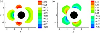
Mapping of the average velocity perturbation
 $\overline{\boldsymbol{u}_{j\rightarrow i}}^{S}$
on the surface of a virtual sphere in the (a) streamwise and (b) spanwise direction.
 $Re_{i}=87$
.

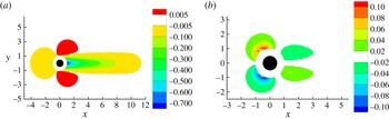
As can be expected the streamwise velocity perturbation at the
 $i$
th particle is negative if it is either in the wake or upstream of the
 $j$
th particle, while the perturbation is weak and positive if it is located laterally. The lateral velocity perturbations at the
 $i$
th particle are stronger from a particle located immediately downstream, but shifted off-axis with respect to the macroscale flow direction. The lateral velocity perturbations due to a downstream located particle is relatively weak. These maps are dependent only on the Reynolds number. Here we show the map for
 $Re=87$
as an example, and the qualitative behaviour remains the same over the Reynolds number range considered. The
 $x$
and
 $y$
extents of the contour plots are chosen such that the surface-averaged perturbation velocity falls to 0.5 % of the incoming uniform ambient flow. Neighbouring spheres located outside these limits would have a negligible effect.
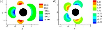
The contour plots of the streamwise and lateral components of the pressure-gradient force integrated over the surface of the particle,
 $-S_{p}\overline{p_{j\rightarrow i}\boldsymbol{n}}^{S}=-V_{p}\overline{\unicode[STIX]{x1D735}\boldsymbol{\cdot }p_{j\rightarrow i}}^{V}$
, are shown in figure 6 as a function of streamwise and lateral separation of the
 $i$
th particle from the
 $j$
th particle (i.e. as a function of
 $r_{x}$
and
 $r_{y}$
). This figure is similar to figure 5 in that the value of the contour for any value of
 $r_{x}$
and
 $r_{y}$
corresponds to pressure force integrated over the surface of the
 $i$
th particle whose centre is located at
 $(r_{x},r_{y})$
, where the perturbation flow is due to the
 $j$
th particle whose centre is located at the origin. These figures can be easily interpreted in conjunction with the perturbation pressure contours shown in figure 4(c). The large stagnation pressure at the front of a downstream neighbour will tend to push the
 $i$
th particle upstream. Similarly the low pressure region in the wake of a downstream neighbour will also tend to push the
 $i$
th particle upstream. The pressure effect of a neighbour located laterally will tend to push the
 $i$
th particle downstream.
Mapping of the pressure-gradient force
 $-V_{p}\overline{\unicode[STIX]{x1D735}\boldsymbol{\cdot }p_{j\rightarrow i}}^{V}$
on a virtual sphere in the (a) streamwise and (b) spanwise direction.
 $Re_{i}=87$
.

In terms of lateral forces, the effect of perturbation pressure due a downstream neighbour is to push the
 $i$
th particle off axis. While the effect of perturbation pressure due an upstream neighbour is to push the
 $i$
th particle towards the axis. The contour plots of the streamwise and lateral components of the viscous force integrated over the surface of the particle,
 $S_{p}\overline{\unicode[STIX]{x1D749}_{j\rightarrow i}\boldsymbol{\cdot }\boldsymbol{n}}^{S}=V_{p}\overline{\unicode[STIX]{x1D735}\boldsymbol{\cdot }\unicode[STIX]{x1D749}_{j\rightarrow i}}^{V}$
, are shown in figure 7 as a function of
 $r_{x}$
and
 $r_{y}$
. In general, these force contributions are smaller in magnitude than the pressure contribution. From figures 6 and 7 it can be seen that the undisturbed flow force due to perturbation flow remains significant only for neighbours located within two diameters.
Mapping of the stress gradient force
 $V_{p}\overline{\unicode[STIX]{x1D735}\boldsymbol{\cdot }\unicode[STIX]{x1D749}_{j\rightarrow i}}^{V}$
on a virtual sphere in the (a) streamwise and (b) spanwise direction.
 $Re_{i}=87$
.

Finally in figure 8 we present contours of volume-averaged vorticity,
 $\overline{\unicode[STIX]{x1D714}_{j\rightarrow i}(x_{i})}^{V}$
, and the streamwise and lateral components of rotational force due to the perturbation flow given by
 $[\overline{\boldsymbol{u}_{mac}}^{V}+\overline{\boldsymbol{u}_{j\rightarrow i}}^{V}]\times \overline{\unicode[STIX]{x1D74E}_{j\rightarrow i}}^{V}$
. As can be expected, rotational force is significant only in case when the
 $i$
th particle is in the vortical wake of an upstream neighbour. Also, the lateral component of the inviscid rotational force is much stronger than the streamwise component. The streamwise component tends to push the
 $i$
th particle downstream, while the lateral force tends to move the particle away from the axis.
Mapping of the (a) vorticity volume average, (b) inviscid rotational force volume average in the streamwise direction and (c) spanwise direction.
 $Re_{i}=87$
.

All the force maps shown in figures 5–8 are for a Reynolds number of 87. The general qualitative description of these maps hold for other Reynolds numbers, but their magnitude and spatial extent somewhat vary. As an example, contours of the streamwise and spanwise component of the undisturbed flow force,
 $S_{p}(-\overline{p_{j\rightarrow i}\boldsymbol{n}}^{S}+\overline{\unicode[STIX]{x1D749}_{j\rightarrow i}\boldsymbol{\cdot }\boldsymbol{n}}^{S})$
, as a function of
 $r_{x}$
and are shown in figure 9 for four different Reynolds numbers. The variation can be seen to be continuous, but complex, for varying Reynolds number. Because of the axisymmetric nature of the simulations it is relatively inexpensive to create these maps for different Reynolds numbers. With small increments of
 $Re$
, a library of the maps shown in figures 5–9 can be created and stored for future application of pairwise interaction model.
Mappings of the inertial force on a virtual sphere in the (a) streamwise and (b) lateral direction for different Reynolds number.

The force maps shown in figures 5–9 are due to one neighbouring particle. For undisturbed flow force, quasi-steady force and added-mass force, from their definitions given in (2.22), (2.23), and (2.24), contributions from each neighbour can be simply added. However, according to its definition given in (2.25), the rotational force contributions from the individual neighbours cannot be simply added. Velocity and vorticity perturbations from individual neighbours must be first added before taking their cross-product.
4 Steady flow through a random array of spheres
Here we present direct numerical simulation of flow over a random array of spheres subjected to a nominally uniform flow at the macroscale. The purpose of these simulations is to test the accuracy of the pairwise interaction model presented in the previous section. Stationary spheres are placed randomly within a rectangular computational box as shown in figure 10. The flow in the streamwise
 $(x)$
and spanwise
 $(y)$
directions are periodic. A no-stress boundary condition is imposed at the top and bottom boundaries in the vertical direction
 $(z)$
. The locations of the centres of the spheres are assigned using a simple random number generator. Two limitations are imposed on the location of the particles: the minimum distance between any two particles should be greater than a few grid cells, and no particle can cross the boundaries in the
 $z$
-direction. A direct forcing immersed boundary method is used to enforce the no-slip and no-penetration conditions on the surface of the spheres. Lagrangian markers are allocated at the surface of the sphere which would generate a forcing
 $\boldsymbol{f}$
on the Cartesian fluid (Eulerian) grid to enforce the no-slip and no-penetration boundary conditions. This forcing is then added to the conservation of momentum equation. The modified Navier–Stokes equations are solved on the Eulerian grid and are given by,
 $$\begin{eqnarray}\displaystyle & \displaystyle \unicode[STIX]{x1D735}\boldsymbol{\cdot }\boldsymbol{u}=0, & \displaystyle\end{eqnarray}$$
 $$\begin{eqnarray}\displaystyle & \displaystyle \frac{\unicode[STIX]{x2202}\boldsymbol{u}}{\unicode[STIX]{x2202}t}+\boldsymbol{u}\boldsymbol{\cdot }\unicode[STIX]{x1D735}\boldsymbol{u}=\unicode[STIX]{x1D735}p+\frac{1}{Re_{a}}\unicode[STIX]{x1D6FB}^{2}\boldsymbol{u}+\boldsymbol{f}. & \displaystyle\end{eqnarray}$$
In these simulations the Reynolds number is defined as
 $Re_{a}=u^{\ast }\text{d}/\unicode[STIX]{x1D708}$
, where
 $u^{\ast }$
is the velocity that would ensure a pressure gradient of unit magnitude in the streamwise direction. A mixed third-order Runge–Kutta and Crank–Nicolson scheme is used to march in time, with a fractional-step method to ensure a divergence free velocity field. The immersed boundary forcing
 $\boldsymbol{f}$
is calculated using the direct method introduced by Uhlmann (Reference Uhlmann2005). At each Runge–Kutta stage, the following equations are solved,
 $$\begin{eqnarray}\displaystyle \tilde{\boldsymbol{u}} & = & \displaystyle \boldsymbol{u}^{(m-1)}+\unicode[STIX]{x1D6FE}_{m}\unicode[STIX]{x0394}t[(\boldsymbol{u}\boldsymbol{\cdot }\unicode[STIX]{x1D735})\boldsymbol{u}]^{(m-1)}\nonumber\\ \displaystyle & & \displaystyle +\,\unicode[STIX]{x1D6FE}_{m}\unicode[STIX]{x1D701}_{m}\unicode[STIX]{x0394}t[(\boldsymbol{u}\boldsymbol{\cdot }\unicode[STIX]{x1D735})\boldsymbol{u}]^{(m-2)}+2\frac{\unicode[STIX]{x1D712}_{m}}{Re}\unicode[STIX]{x1D6FB}^{2}\boldsymbol{u}^{(m-1)}-2\unicode[STIX]{x1D712}_{m}\unicode[STIX]{x1D735}p^{(m-1)}\end{eqnarray}$$
 $$\begin{eqnarray}\displaystyle & \displaystyle \tilde{\boldsymbol{U}}(\boldsymbol{X}_{l})=\mathop{\sum }_{\forall \boldsymbol{x}}\tilde{\boldsymbol{u}}(x)\unicode[STIX]{x1D6FF}(\boldsymbol{x}-\boldsymbol{X}_{l})\,\text{d}v(\boldsymbol{x}) & \displaystyle\end{eqnarray}$$
 $$\begin{eqnarray}\displaystyle & \displaystyle \boldsymbol{F}(\boldsymbol{X}_{l})=\frac{\boldsymbol{U}(\boldsymbol{X}_{l})^{(d)}-\tilde{\boldsymbol{U}}(\boldsymbol{X}_{l})}{\unicode[STIX]{x0394}t} & \displaystyle\end{eqnarray}$$
 $$\begin{eqnarray}\displaystyle & \displaystyle \boldsymbol{f}(\boldsymbol{x})=\mathop{\sum }_{n=1}^{N_{p}}\mathop{\sum }_{l=1}^{N_{L}(n)}\boldsymbol{F}(\boldsymbol{X}_{l})\unicode[STIX]{x1D6FF}(\boldsymbol{x}-\boldsymbol{X}_{l})\unicode[STIX]{x0394}V_{l}, & \displaystyle\end{eqnarray}$$
where
 $m$
represents the Runge–Kutta stage. The coefficient of diffusion
 $\unicode[STIX]{x1D712}_{m}$
, coefficient of first nonlinear term
 $\unicode[STIX]{x1D6FE}_{m}$
, and coefficient of second nonlinear term
 $\unicode[STIX]{x1D701}_{m}$
are characteristic of the temporal scheme used (Canuto et al.
Reference Canuto, Hussaini, Quarteroni and Zang1988; Cortese & Balachandar Reference Cortese and Balachandar1995). Equation (4.4) interpolates the fluid velocity from the Eulerian grid onto the Lagrangian markers positioned at
 $\boldsymbol{X}$
. The interpolation step employs a discrete delta function and the weight of each Eulerian grid point is its corresponding volume
 $\text{d}v$
. The Lagrangian forcing
 $\boldsymbol{F}$
at each Lagrangian marker is calculated using (4.5) where
 $\boldsymbol{U}^{(d)}$
is the desired velocity at the Lagrangian marker, which is set to zero in this study of stationary distribution of spheres. The Lagrangian forcing is then projected onto the Eulerian grid using (4.6) where
 $\unicode[STIX]{x0394}V$
is the Lagrangian weight.
Schematic of the geometry for a random array of monodisperse spheres.

The Eulerian grid is uniform in the streamwise and spanwise direction. In the
 $z$
-direction, a non-uniform grid is defined as,
 $$\begin{eqnarray}\displaystyle z_{k}=\frac{\arcsin \displaystyle \left(\unicode[STIX]{x1D6FC}\cos \left((k-1)\frac{\unicode[STIX]{x03C0}}{N_{z}-1}\right)\right)}{\arcsin (\unicode[STIX]{x1D6FC})}\quad 1\leqslant k\leqslant N_{z}\text{ and }0\leqslant \unicode[STIX]{x1D6FC}<1. & & \displaystyle\end{eqnarray}$$
For
 $\unicode[STIX]{x1D6FC}=0$
, the distribution follows the Chebyshev–Gauss–Lobatto point distribution. For
 $\unicode[STIX]{x1D6FC}=1$
, the distribution is uniform. For this study,
 $\unicode[STIX]{x1D6FC}$
is set to 0.99 leading to a nearly uniform distribution. The correction given by Pinelli et al. (Reference Pinelli, Naqavi, Piomelli and Favier2010) for non-uniform grids is used here. A non-uniform distribution of Lagrangian markers, as presented by Akiki & Balachandar (Reference Akiki and Balachandar2016), is used to achieve an optimal number and distribution of Lagrangian markers. The Lagrangian weights
 $\unicode[STIX]{x0394}V$
are evaluated using the vector spherical harmonics technique proposed by Akiki & Balachandar (Reference Akiki and Balachandar2016). Only the spheres lying in the middle 64 % of the domain in the
 $z$
-direction will be considered, in order to reduce the effect of the stress-free walls on the hydrodynamic forces within the array. The overall numerical scheme has been extensively validated, for single and multiple spheres, in both ordered and random arrays (see Akiki & Balachandar Reference Akiki and Balachandar2016).
Flow past an array of particles is achieved by imposing a non-dimensional pressure gradient of unity in the
 $x$
-direction. The volumetric flow rate, and therefore the non-dimensional average velocity in the fluid phase
 $u_{f}$
, are obtained a posteriori as,
 $$\begin{eqnarray}\displaystyle u_{f}=\frac{\displaystyle \int _{\unicode[STIX]{x1D6FA}}I_{f}(\boldsymbol{x})u(\boldsymbol{x})\,\text{d}\boldsymbol{x}}{\displaystyle \int _{\unicode[STIX]{x1D6FA}}I_{f}(\boldsymbol{x})\,\text{d}\boldsymbol{x}}, & & \displaystyle\end{eqnarray}$$
where
 $\unicode[STIX]{x1D6FA}$
is the volume containing all the spheres that are being considered, and
 $I_{f}$
is the fluid indicator defined as,
 $$\begin{eqnarray}\displaystyle \left.\begin{array}{@{}c@{}}\displaystyle I_{f}(\boldsymbol{x})=1,\quad \text{if }\boldsymbol{x}\text{ is in the fluid phase,}\\ \displaystyle I_{f}(\boldsymbol{x})=0,\quad \text{if }\boldsymbol{x}\text{ is in the solid phase.}\end{array}\right\} & & \displaystyle\end{eqnarray}$$
The macroscale particle Reynolds number is then calculated using the average velocity as,
 $$\begin{eqnarray}\displaystyle Re=u_{f}Re_{a}, & & \displaystyle\end{eqnarray}$$
which remains the same for all the particles. The individual non-dimensional force on each particle is calculated through the integration of the immersed boundary forcing
 $\boldsymbol{F}$
obtained from (4.5),
 $$\begin{eqnarray}\displaystyle \boldsymbol{F}_{DNS}(n)=\frac{1}{u_{f}^{2}}\mathop{\sum }_{l=1}^{N_{L}(n)}\boldsymbol{F}(\boldsymbol{X}_{l})\unicode[STIX]{x0394}V_{l}, & & \displaystyle\end{eqnarray}$$
where
 $N_{L}(n)$
is the total number of Lagrangian markers on the
 $n$
th sphere.
5 Results
5.1 PIEP model forces versus DNS results
A series of DNS simulations for different distributions of monodisperse spherical particles with different volume fractions and Reynolds numbers are conducted using the numerical method outlined in § 4. Table 1 contains the parameters of the cases explored. Each case has been repeated for different random arrangements. The number of realizations (NOR) performed for each of the cases is included in table 1. The force
 $\boldsymbol{F}_{DNS}$
as computed using (4.11) is projected along the direction of mean flow (i.e. along the
 $x$
direction) to obtain the drag force and the perpendicular component is termed the lateral (or lift) force.
Parameters of the DNS of the array of particles.

We now define the mean drag for a random distribution of spheres to be the drag force averaged over an ensemble of randomly distributed particles under identical volume fraction and macroscale Reynolds number. Averaging the force model (2.26) over an ensemble of particles we obtain
 $$\begin{eqnarray}\displaystyle \langle F_{x}\rangle =\langle F_{x,un}\rangle +\langle F_{x,qs}\rangle , & & \displaystyle\end{eqnarray}$$
since the ensemble averages of added-mass, Basset history and rotational forces are zero. Here and henceforth ‘
 $x$
’ in the subscript indicates the streamwise (or drag) component of force and ‘
 $n$
’ in the subscript indicates the lateral (or lift) component. The ensemble-averaged undisturbed flow force is only due to the mean macroscopic pressure gradient. Under steady conditions, the macroscale pressure gradient is balanced by the mean drag and as a result (see Tang et al.
Reference Tang, Peters, Kuipers, Kriebitzsch and Hoef2015)
 $$\begin{eqnarray}\displaystyle \langle F_{x,un}\rangle =-V_{p}\overline{\unicode[STIX]{x1D735}\boldsymbol{\cdot }p_{j\rightarrow i}}^{V}=\unicode[STIX]{x1D719}\langle F_{x}\rangle . & & \displaystyle\end{eqnarray}$$
The mean quasi-steady drag force on a random distribution of spheres will be taken to be the following volume fraction-dependent drag law by Tenneti et al. (Reference Tenneti, Garg and Subramaniam2011),
 $$\begin{eqnarray}\displaystyle \langle F_{x,qs}\rangle =F_{ra} & = & \displaystyle \frac{3\unicode[STIX]{x03C0}(1-\unicode[STIX]{x1D719})}{Re_{s}}\left[\frac{1+0.15Re_{s}^{0.687}}{(1-\unicode[STIX]{x1D719})^{3}}+\frac{5.81\unicode[STIX]{x1D719}}{(1-\unicode[STIX]{x1D719})^{3}}\right.\nonumber\\ \displaystyle & & \displaystyle \left.+\,0.48\frac{\unicode[STIX]{x1D719}^{1/3}}{(1-\unicode[STIX]{x1D719})^{4}}+\unicode[STIX]{x1D719}^{3}Re_{s}\left(0.95+\frac{0.61\unicode[STIX]{x1D719}^{3}}{(1-\unicode[STIX]{x1D719})^{2}}\right)\right],\end{eqnarray}$$
where
 $Re_{s}$
is the Reynolds number based on the superficial velocity,
 $$\begin{eqnarray}\displaystyle Re_{s}=\frac{Re}{(1-\unicode[STIX]{x1D719})}. & & \displaystyle\end{eqnarray}$$
From the above equations, the mean pressure-gradient force can be expressed in terms of the mean quasi-steady force, and the mean drag force becomes
 $$\begin{eqnarray}\displaystyle \langle F_{x}\rangle =\langle F_{x,un}\rangle +\langle F_{x,qs}\rangle =\frac{\unicode[STIX]{x1D719}}{1-\unicode[STIX]{x1D719}}F_{ra}+F_{ra}=\frac{F_{ra}}{1-\unicode[STIX]{x1D719}}. & & \displaystyle\end{eqnarray}$$
Figure 11 shows a scatter plot of the actual drag force (i.e.
 $F_{x,DNS}=\boldsymbol{F}_{DNS}\boldsymbol{\cdot }\boldsymbol{e}_{x}$
) obtained from the DNS simulation for case vf1re1 versus drag force as predicted by the above volume fraction-dependent mean drag model. The drag law recovers extremely well the mean drag obtained from DNS where the difference is only 0.16 % for the case shown. But the mean drag model fails to capture the wide variation of the drag forces experienced by the different spheres. Each model will be assessed using the following definition of
 $R^{2}$
as the statistical measure of how well the model prediction is in agreement with the actual DNS data:
 $$\begin{eqnarray}\displaystyle R^{2}=1-\frac{\displaystyle \mathop{\sum }_{n=1}^{N_{p}}[F_{x,DNS}(n)-F_{x,Model}(n)]^{2}}{\displaystyle \mathop{\sum }_{n=1}^{N_{p}}[F_{x,DNS}(n)-\langle F_{x,DNS}\rangle ]^{2}}, & & \displaystyle\end{eqnarray}$$
where
 $\langle F_{x,DNS}\rangle$
is the ensemble average of the DNS drag. A perfect model would have all the data points fall on the bisector shown alongside in figure 11 for reference. The mean drag model and the perfect model present the limiting cases, where the mean drag model has a correlation of
 $R^{2}=0$
and the perfect model has a value of
 $R^{2}=1$
.
Scatter plot of the drag obtained on 108 spheres from the DNS simulations of case vf1re1 versus the mean drag law by Tenneti et al. (Reference Tenneti, Garg and Subramaniam2011). The solid line is the first bisector
 $y=x$
.

5.1.1 Drag force
For each random distribution of spheres used in the fully resolved simulations listed in table 1, we apply the PIEP model to calculate the drag on each individual sphere within the array. Note that the drag is defined as the component of force in the
 $x$
-direction rather than in the direction of the local streamline. For each sphere we calculate the drag force as,
 $$\begin{eqnarray}\displaystyle F_{x,PIEP}=F_{x,un}+F_{x,qs}+F_{x,am}+F_{x,L}. & & \displaystyle\end{eqnarray}$$
The added-mass forces will be combined with the undisturbed flow force and reported together, since both forces have the same form. The terms on the right-hand side of (5.7) are computed using (2.22), (2.23), (2.24) and (2.25), respectively. As an example, scatter plots of the DNS drag against each of the three components of the PIEP model (i.e.
 $F_{x,un}+F_{x,am}$
,
 $F_{x,qs}$
and
 $F_{x,L}$
) are shown in the first three scatter plots of figure 12 for the case of vf1re1. The mean value of
 $F_{x,PIEP}$
is in good agreement with the mean DNS drag (see table 2). Therefore, to facilitate fair comparison in the first three frames of figure 12 only the scatter plot of deviation from the mean value is plotted.
DNS drag versus (a) the unsteady and added-mass forces, (b) the quasi-steady force, (c) inviscid rotational force and (d) PIEP drag force for case vf1re1. The first three frames show the force deviation from the mean and the fourth frame shows the total force. The solid line is the first bisector
 $y=x$
.

Mean and standard deviation introduced by each component of the PIEP model, the total PIEP drag force and the DNS drag force. The last column shows the correlation between the PIEP force and the DNS force.

It can be observed that all three scatter plots are tilted towards the bisector, indicating that all three components of the PIEP model correctly predict increased (or decreased) drag for particles whose actual DNS drag was higher (or lower) than the mean. The contribution from the inviscid rotational force component of the PIEP model is quite small. In contrast, the quasi-steady component of the PIEP model accounts for a large portion of the particle-to-particle variation in the DNS drag force. This suggests that the increase (or decrease) in the DNS drag force on a particle within the random array depends largely on whether the undisturbed flow velocity averaged over the surface of the particle is higher (or lower) due to the channelling of flow (or blocking of flow) by the neighbouring particles. The effect of pressure distribution and viscous stresses is smaller than the quasi-steady contribution, but its contribution is significant and cannot be ignored. The sum of the three contributions forms the total prediction by the PIEP model and it is plotted in frame (d) against the DNS drag force. Unlike the first three frames, the mean has not been subtracted in frame (d). Based on
 $R^{2}$
measure the PIEP model is able to capture 75 % of the particle-to-particle variation in the drag force. The prediction from the PIEP model is not perfect, as there is still some scatter in the data. Given the approximations involved in the PIEP model, the lack of perfect correlation between its prediction and the PIEP model is to be expected. Nevertheless, the improvement over the best available volume fraction-dependent drag model shown in figure 11 is quite promising.
Table 2 presents the statistical information on the mean and standard deviation of the drag component of
 $F_{x,un}+F_{x,am}$
,
 $F_{x,qs}$
,
 $F_{x,L}$
and their sum, which is the drag force predicted by the PIEP model. For comparison, also presented in table 2 are the mean and standard deviation of the DNS drag for the four cases considered in this study. It can be observed that the mean DNS drag is well predicted by the PIEP model. The table shows that the standard deviation for the lower volume fraction cases matches well with the DNS data. For the higher volume fraction, the PIEP model is able to account for approximately 50 % of the actual standard deviation. At higher volume fractions, higher-order interaction perhaps becomes more prominent. These interactions may contribute to additional variations which are not accounted for in a pairwise interaction model.
The results of the individual contribution of each term of (5.7) shown in table 2 reveal that the rotational force has a negligible effect for all cases considered. The quasi-steady force accounts for the dominant portion of both the mean and the standard deviation of the drag force for all cases. The undisturbed flow force has an increasing effect as the Reynolds number increases. At lower Reynolds numbers the standard deviation of
 $F_{un}$
accounts for approximately 20 % of the DNS standard deviation and this percentage increases to 40 % at the higher Reynolds number.
Limiting the number of neighbours. The expressions for the different components of
 $F_{x,PIEP}$
given in (2.22), (2.23), (2.24) and (2.25) involve summation over perturbations from all the other spheres within the array. For the results presented in the above sections we systematically summed over all the neighbours, which in the cases of
 $\unicode[STIX]{x1D719}=0.1$
and 0.21 involve summing over 107 and 214 neighbouring spheres, respectively. From a practical point of view, the vast majority of these spheres are far away and as indicated in the force maps have negligible effects on the perturbation force. Rather than including the perturbation force contribution from all the other spheres within the array, we can limit the summation to only spheres that are located within a larger ball of radius
 $\unicode[STIX]{x1D712}$
centred about the sphere
 $i$
. Limiting the radius of influence to
 $\unicode[STIX]{x1D712}$
leads to a substantial reduction in the computational cost with no significant impact on the effectiveness of the model.
The radius of influence around each sphere is now varied from 1 to 4.5 times the sphere diameter. For each
 $\unicode[STIX]{x1D712}$
, equation (5.7) of the PIEP model was evaluated using only the spheres falling within a distance
 $\unicode[STIX]{x1D712}$
. The resulting drag forces are then assessed using the same method of scatter plots and
 $R^{2}$
values presented in figure 12. Figure 13 shows the plots of
 $R^{2}$
versus
 $\unicode[STIX]{x1D712}$
for all the four cases listed in table 1. For each case, the results from different realizations are shown separately, where each realization is denoted by a seed number. For all the cases, a steep increase in correlation is observed by including only the first few nearest neighbours. A good correlation is obtained by only including neighbouring spheres within
 $\unicode[STIX]{x1D712}=2.5$
for
 $\unicode[STIX]{x1D719}=0.1$
and less than 2 for
 $\unicode[STIX]{x1D719}=0.2$
. For the cases of
 $\unicode[STIX]{x1D719}=0.1$
, a continued increase in
 $R^{2}$
value is observed as more spheres are included past
 $\unicode[STIX]{x1D712}=2.5$
. For the two cases of
 $\unicode[STIX]{x1D719}=0.2$
, increasing the radius of influence to more than
 $\unicode[STIX]{x1D712}=2$
does not lead to any substantial increase in correlation. The maximum
 $R^{2}$
is seen to decrease with increasing Reynolds number. The interaction of the spheres with their upstream neighbourhood mediated through the complex flow modification of the continuous phase is magnified with increasing
 $Re$
. This interaction increases the error in the pairwise interaction assumption and thereby contributes to lower
 $R^{2}$
value. Nonetheless, the correlations obtained, even for the highest particle Reynolds number of 170, are in excess of 0.5, which reflects a substantial improvement in the deterministic prediction of drag.
 $R^{2}$
of the PIEP drag force versus radius of influence for (a) vf1re1, (b) vf1re2, (c) vf2re1 and (d) vf2re2.

An extra case of
 $\unicode[STIX]{x1D719}=0.2$
and
 $Re=357$
was also tested. At that Reynolds number, the flow inside the array is unsteady, even though a constant pressure gradient was applied across the periodic array. Figure 14 shows the instantaneous drag on select spheres within the array as a function of time. The instantaneous drag variation is not due to the time-dependent nature of macroscale flow (it remains steady and uniform). The temporal variation in the drag force of each particle is due to chaotic vortex shedding in the wave. In the case of a random array, self-induced vortex shedding, along with the time-dependent perturbation flow from the neighbouring particles, influence the fluctuating drag. This time variation in drag force cannot be predicted by the PIEP model. For the three spheres shown in figure 14, the time-averaged drag force are 0.75 (red curve), 0.48 (green curve) and 0.87 (blue curve). For the whole array, the time-averaged drag has a mean of
 $\langle F_{x,DNS}\rangle =0.65$
. It is interesting to note that particle-to-particle variation in the time-averaged drag is substantially larger than the temporal fluctuation.
Instantaneous drag on three select individual spheres versus time. The spheres are part of an array where
 $\unicode[STIX]{x1D719}=0.2$
and
 $Re=357$
. The mean drag of the array is
 $\langle F_{DNS}\rangle =0.65$
. The time average drags on the three spheres are 0.75 (red), 0.48 (green) and 0.87 (blue).

At
 $Re=357$
even the flow over an isolated particle is time dependent. Therefore, the mappings of the PIEP model are created based on the time-averaged flow (refer to § 3.2). The results of the PIEP model drag force versus the time-averaged DNS drag are shown in the scatter plot of figure 15. A correlation of 0.45 is obtained with an overall standard deviation of the PIEP model drag being 80 % of the standard deviation of the particle-to-particle time-averaged DNS drag variation. The
 $R^{2}$
value, although lower than the ones obtained for lower Reynolds numbers, still presents a significant reduction in the error when compared to the volume fraction-dependent mean drag model. The decrease in correlation is attributed to the increased level of higher-order interaction between spheres.
DNS drag versus PIEP force model for case
 $\unicode[STIX]{x1D719}=0.2$
and
 $Re=357$
.

5.1.2 Lateral force
The lateral forces within an array of fixed spheres are shown to be very significant by Akiki et al. (Reference Akiki, Jackson and Balachandar2016). For the range of volume fraction and Reynolds number of this study, the lateral force is approximately 15 % of the mean drag. In the present context of a uniform macroscale flow oriented along the
 $x$
-direction, the source of the lateral force is entirely due to the perturbation flow induced by the neighbours. In the presence of macroscale shear and vorticity there will be additional contribution to lateral force from Saffman and Auton-type lift forces and similarly if the spheres are allowed to rotate there will be additional Magnus lift force. Even in the case of a uniform flow through a fixed bed of spheres, particle–particle interaction mediated through the continuous phase flow results in substantial force in the lateral direction.
A detailed knowledge of the local flow direction, magnitude, and vorticity is needed to obtain the actual lateral force. But this information is not available if the problem is considered at the macroscale. With information limited to only macroscale Reynolds number and mean volume fraction within the array, the best estimation of the lateral force is zero, which indeed is an accurate prediction of the expected mean value of the lift force. PIEP model has the potential to provide a better approximation of the direction and magnitude of the lateral force on individual particles, provided the locations of the neighbouring spheres are known. The PIEP model will implicitly account for the complex undisturbed flow that exists at each of the particle due to the perturbation flow induced by all its neighbours, without having to explicitly solve for this local flow information. For each sphere, the lateral force along the
 $y$
- and
 $z$
-directions are calculated as,
 $$\begin{eqnarray}\displaystyle F_{y,PIEP}=F_{y,un}+F_{y,qs}+F_{y,am}+F_{y,L}\quad \text{and}\quad F_{z,PIEP}=F_{z,un}+F_{z,qs}+F_{z,am}+F_{z,L}. & & \displaystyle \nonumber\\ \displaystyle & & \displaystyle\end{eqnarray}$$
Note that in the lateral force case, the finite volume fraction correlation
 $F_{ra}$
used in (2.23) is set to zero. Here, we show the results for the
 $y$
-direction in the remainder of the analysis. The results are equally valid for the
 $z$
-direction.
Similar to figure 12, a scatter plot of the components
 $F_{y,un}+F_{y,am}$
,
 $F_{y,qs}$
and
 $F_{y,L}$
of (5.8a
) are shown separately in the first three frames of figure 16 for the case vf2re1. The fourth frame contains the scatter plot of the total lateral force obtained from the PIEP model plotted versus the DNS
 $y$
-force. It should be recognized that the forces along the
 $y$
- and the
 $z$
-directions are lateral forces (or lift fo rces) only in the sense of the macroscale flow. In fact, from its definition
 $F_{y,qs}$
is clearly a drag force as it is directed in the direction of the local undisturbed flow. Only the rotational force is strictly a lift force, directed normal to the local undisturbed flow. The rotational force scatter plot reveals that its contribution to the lateral force is again quite small and can be ignored. The added-mass and the quasi-steady force predictions tend to align in direction with the actual lateral force, but the predicted magnitude is smaller compared to the DNS results. The fourth frame in figure 16 shows the scatter plot of the total
 $y$
-force. It can be seen that the model results in only a modest correlation of
 $R^{2}=0.32$
, which is considerably lower than that obtained for the drag force. From the tilt of the scatter plots towards the bisector it can be seen that the PIEP model given in (5.8) is able to predict the direction of the lateral force. However, the PIEP model underestimates the magnitude of the actual lateral force.
DNS lift versus PIEP lift model using (a) inviscid irrotational, (b) quasi-steady, (c) inviscid rotational and (d) all forces for case vf2re1.

Table 3 presents the statistical information on the mean and standard deviation as well as
 $R^{2}$
of the
 $y$
-component of force,
 $F_{y,un}+F_{y,am}$
,
 $F_{y,qs}$
,
 $F_{y,L}$
, and their sum which is the PIEP prediction of the lateral force. Also presented in table 3 are the mean and standard deviation of the DNS lateral force for the four cases considered. It can be observed that the mean DNS lateral force along with the mean PIEP model prediction are close to zero (due to limited sample size, the mean values are not perfectly zero). For all cases, the quasi-steady force returns the highest correlation with the DNS values. The other forces show low to zero correlation for all cases. By comparing the standard deviation of the PIEP forces and the DNS forces, it is clear that the current model is not able to fully account for the actual variation of the lift force within the array.
Mean, standard deviation and correlation introduced by each component of the PIEP model, as well as the total PIEP lift force in the
 $y$
-direction. The last two columns contain the mean and standard deviation of the DNS lift forces.

Figure 17 shows the evolution of
 $R^{2}$
as the radius of influence
 $\unicode[STIX]{x1D712}$
is increased. The lower Reynolds number cases (vf1re1 and vf2re1) show a reasonable correlation by including spheres located within 1.5 diameters of each sphere. This is lower than the minimum radius of influence required for the drag. But in general, the value of
 $R^{2}$
is lower for the lateral force compared to the correlations obtained for the drag. The correlation decreases for the higher Reynolds number of vf2re2 where the combination of the higher volume fraction and Reynolds number deteriorates the accuracy of the pairwise interaction assumption. For the case of vf1re2, the correlation is zero for all values of
 $\unicode[STIX]{x1D712}$
. Referring back to table 3, a correlation of 0.3 is observed for case vf1re2 when using the quasi-steady force only. This correlation is driven down to zero when including the other forces. The main reason of the lack of correlation is the large uncorrelated contribution from
 $F_{y,un}+F_{y,am}$
. Using the quasi-steady force contribution only when applying the PIEP model for predicting the lateral force is a viable option at higher Reynolds numbers.
5.2 On the practical implementation of PIEP
The mean value (or ensemble average) of the quasi-steady force given by (2.23) can be expressed as
 $$\begin{eqnarray}\displaystyle \langle \boldsymbol{F}_{qs}\rangle =\boldsymbol{F}_{ra}(\unicode[STIX]{x1D719},Re)+\left\{3\unicode[STIX]{x03C0}\unicode[STIX]{x1D707}d\left\langle \mathop{\sum }_{\substack{ j=1 \\ j\neq i}}^{N}\overline{\boldsymbol{u}_{j\rightarrow i}}^{S}(x_{i})\right\rangle [1+0.15(Re)^{0.687}]\right\}. & & \displaystyle\end{eqnarray}$$
 $R^{2}$
of the PIEP lateral force versus
 $r$
for vf1re1, vf1re2, vf2re1 and vf2re2.

The first part corresponds to the mean quasi-steady force due to the macroscale flow, while the second part is the contribution to the mean quasi-steady drag from the perturbation flow induced by the neighbours. When perturbation flow due to the neighbours is summed over all the neighbours then the second term on the right-hand side approaches zero, since
 $$\begin{eqnarray}\displaystyle \left\langle \mathop{\sum }_{\substack{ j=1 \\ j\neq i}}^{N}\overline{\boldsymbol{u}_{j\rightarrow i}}^{S}(x_{i})\right\rangle =0. & & \displaystyle\end{eqnarray}$$
As pointed out earlier, in a practical implementation of the PIEP model it is necessary to limit the number of neighbours to those within a larger sphere of radius
 $\unicode[STIX]{x1D712}$
. Let
 $n(\unicode[STIX]{x1D712})$
be the number of neighbouring spheres within a ball of radius
 $\unicode[STIX]{x1D712}$
centred about the reference sphere, whose mean value for a random distribution of particles with uniform probability can be estimated to be
 $$\begin{eqnarray}\displaystyle \langle n(\unicode[STIX]{x1D712})\rangle =8(\unicode[STIX]{x1D712}^{3}-1)\unicode[STIX]{x1D719}. & & \displaystyle\end{eqnarray}$$
For a finite
 $\unicode[STIX]{x1D712}$
, the second term of (5.9) is not guaranteed to be zero and in general for the streamwise component we can expect
 $$\begin{eqnarray}\displaystyle \left\langle \mathop{\sum }_{\substack{ j=1 \\ j\neq i}}^{n(\unicode[STIX]{x1D712})}\overline{\boldsymbol{u}_{j\rightarrow i}}^{S}(x_{i})\right\rangle \boldsymbol{\cdot }\boldsymbol{e}_{x}=f(\unicode[STIX]{x1D719},Re,\unicode[STIX]{x1D712}), & & \displaystyle\end{eqnarray}$$
where the non-zero value will be a function of the volume fraction, Reynolds number and the size of the ball of influence. As
 $\unicode[STIX]{x1D712}\rightarrow \infty$
we expect
 $f(\unicode[STIX]{x1D719},Re,\unicode[STIX]{x1D712})\rightarrow 0$
. However, for finite values of
 $\unicode[STIX]{x1D712}$
the mean value of the quasi-steady force predicted with the PIEP model will be corrupted by the second term of (5.9) and will differ from the actual mean. Due to symmetry the lateral component of
 $\langle \sum _{\substack{ j=1 \\ j\neq i}}^{n(\unicode[STIX]{x1D712})}\overline{\boldsymbol{u}_{j\rightarrow i}}^{S}(x_{i})\rangle$
will remain zero irrespective of the size of the region of influence used in the PIEP model.
In the streamwise direction, the non-zero value of
 $\langle \sum _{\substack{ j=1 \\ j\neq i}}^{n(\unicode[STIX]{x1D712})}\overline{\boldsymbol{u}_{j\rightarrow i}}^{S}(x_{i})\rangle$
is due to the nature of the perturbation streamwise velocity shown in figure 4(a). In the figure it can be seen that the negative velocity perturbation (velocity less than the free stream velocity of unity) is strong and extends upstream and downstream of the particle. The negative velocity is compensated by a weak positive velocity that extends over a very large region. Thus, averaging the velocity perturbation over a ball of finite radius will result in a net non-zero (negative) value. In evaluating
 $f(\unicode[STIX]{x1D719},Re,\unicode[STIX]{x1D712})$
it must be recognized that, due to the finite size of the particles, the probability of finding a neighbour at any given distance from the reference particle will depend on the pair probability function, which is related to the radial distribution function. The function
 $f(\unicode[STIX]{x1D719},Re,\unicode[STIX]{x1D712})$
can be written as,
 $$\begin{eqnarray}\displaystyle f(\unicode[STIX]{x1D719},Re,\unicode[STIX]{x1D712})=\frac{2\unicode[STIX]{x03C0}}{\frac{4}{3}\unicode[STIX]{x03C0}(\unicode[STIX]{x1D712}^{3}-d^{3})}\int _{0}^{\unicode[STIX]{x03C0}}\int _{d}^{\unicode[STIX]{x1D712}}g(\unicode[STIX]{x1D719},r^{\prime })\overline{\boldsymbol{u}_{j\rightarrow i}}^{S}(Re,\unicode[STIX]{x1D703},r^{\prime }){r^{\prime }}^{2}\sin \unicode[STIX]{x1D703}\,\text{d}r^{\prime }\,\text{d}\unicode[STIX]{x1D703}. & & \displaystyle\end{eqnarray}$$
The function
 $g(\unicode[STIX]{x1D719},r^{\prime })$
is the radial distribution function, and it measures the probability of the presence of a neighbouring sphere at a distance
 $r^{\prime }$
from the reference sphere. There is no closed form solution for
 $g(\unicode[STIX]{x1D719},r^{\prime })$
and it is usually computed using the Monte Carlo method or using the Ornstein–Zernike equation (Ornstein & Zernike Reference Ornstein and Zernike1914). Here we use an exact solution of the Percus–Yevick approximation (Percus & Yevick Reference Percus and Yevick1958; Wertheim Reference Wertheim1963) to obtain
 $g$
(
 $\unicode[STIX]{x1D719}$
,
 $r$
). For a finite
 $\unicode[STIX]{x1D712}$
, equation (2.23) must be modified as follows,
 $$\begin{eqnarray}\displaystyle \boldsymbol{F}_{qs}=\boldsymbol{F}_{ra}(\unicode[STIX]{x1D719},Re_{i})+\left\{3\unicode[STIX]{x03C0}\unicode[STIX]{x1D707}d\left(\mathop{\sum }_{\substack{ j=1 \\ j\neq i}}^{n(\unicode[STIX]{x1D712})}(\overline{\boldsymbol{u}_{j\rightarrow i}}^{S}(x_{i})-f(\unicode[STIX]{x1D719},Re,\unicode[STIX]{x1D712}))\right)[1+0.15(Re_{i})^{0.687}]\right\}, & & \displaystyle \nonumber\\ \displaystyle & & \displaystyle\end{eqnarray}$$
in order to obtain the correct mean drag force.
5.2.1 Empirical improvements
In figure 18 the probability distribution of the difference between the DNS drag and that predicted with the PIEP model (i.e. the probability density function (PDF) of (
 $F_{x,DNS}$
–
 $F_{x,PIEP}$
)) is plotted. It was observed in Akiki et al. (Reference Akiki, Jackson and Balachandar2016) that the deviation of the actual drag force on the individual particles from the mean value
 $(\langle F_{x}\rangle )$
followed a Gaussian distribution of zero mean, whose standard deviation is listed as
 $\unicode[STIX]{x1D70E}_{F_{x,DNS}}$
in table 2. To capture the particle-to-particle drag variation within the random distribution of particles they introduced a simple stochastic additive contribution to compute the force
 $F_{d}$
on an individual particle. The stochastic contribution is defined as a random variable chosen from a normal distribution of zero mean and specified standard deviation. The resulting stochastic drag model is given by
 $$\begin{eqnarray}\displaystyle F_{x,ST}=\langle F_{x}\rangle (Re,\unicode[STIX]{x1D719})+N(0,\unicode[STIX]{x1D70E}_{F_{x}}(Re,\unicode[STIX]{x1D719})), & & \displaystyle\end{eqnarray}$$
where it is recognized that both the mean and the standard deviation are functions of both the mean Reynolds number and the mean volume fraction. The above stochastic model will ensure a drag distribution whose statistical properties match those of the actual DNS drag distribution. However, since
 $$\begin{eqnarray}\displaystyle \langle (F_{x,DNS}-F_{x,ST})^{2}\rangle =\langle (F_{x,DNS}-\langle F_{x}\rangle )^{2}\rangle +\langle N^{2}\rangle =2\langle (F_{x,DNS}-\langle F_{x}\rangle )^{2}\rangle & & \displaystyle\end{eqnarray}$$
the standard deviation of the resulting stochastic prediction from the actual DNS drag force would increase by factor
 $\sqrt{2}$
.
Probability distribution of the difference between the DNS and predicted drag force.

With the PIEP model a substantial portion of the particle-to-particle drag variation has already been captured deterministically. As seen in table 2 the standard deviation of the PIEP prediction from the mean value is somewhat lower than the standard deviation of the actual DNS drag. One simple empirical approach to match the standard deviation is to modify the PIEP model as follows
 $$\begin{eqnarray}\displaystyle F_{x,PIEP2}=\langle F_{x}\rangle +\unicode[STIX]{x1D6FD}(F_{x,PIEP}-\langle F_{x}\rangle ). & & \displaystyle\end{eqnarray}$$
The above modification simply scales the deviation from mean by a factor
 $\unicode[STIX]{x1D6FD}$
. This modification leaves the mean unaltered, which is already in agreement with the actual mean. But the standard deviation of
 $F_{x,PIEP2}$
is
 $\unicode[STIX]{x1D6FD}$
times the standard deviation of
 $F_{x,PIEP}$
and therefore by choosing
 $$\begin{eqnarray}\displaystyle \unicode[STIX]{x1D6FD}=\frac{\unicode[STIX]{x1D70E}_{x,DNS}}{\unicode[STIX]{x1D70E}_{x,PIEP}}. & & \displaystyle\end{eqnarray}$$
The standard deviation of
 $F_{x,PIEP2}$
can be matched with that of the DNS data. In this approach, we do not need to introduce an additional stochastic component as in (5.15), which tends to double the r.m.s. deviation from the actual drag. Here we exploit the fact that the PIEP model correctly predicts which particles have higher or lower than the mean drag and that the PIEP model only under predicts the magnitude of this deviation. The empirical factor
 $\unicode[STIX]{x1D6FD}$
is intended to scale up the level of deviation, so that both the mean and standard deviations can be matched. As far as the difference between the predicted drag
 $F_{x,PIEP2}$
and the actual DNS drag, by definition the mean values is in agreement and the variance can be expressed as
 $$\begin{eqnarray}\displaystyle \langle (F_{x,DNS}-F_{x,PIEP2})^{2}\rangle & = & \displaystyle \langle (F_{x,DNS}-\langle F_{x}\rangle )^{2}\rangle -2\unicode[STIX]{x1D6FD}\langle (F_{x,DNS}-\langle F_{x}\rangle )(F_{x,PIEP2}-\langle F_{x}\rangle )\rangle \nonumber\\ \displaystyle & & \displaystyle +\,\langle (F_{x,PIEP2}-\langle F_{x}\rangle )^{2}\rangle .\end{eqnarray}$$
Here we note that the deviation from the mean predicted by the PIEP model
 $(F_{x,PIEP2}-\langle F_{x}\rangle )$
is very well correlated with
 $(F_{x,DNS}-\langle F_{x}\rangle )$
. In general, the PIEP model will not be perfect, i.e.
 $\langle (F_{x,DNS}-F_{x,PIEP2})^{2}\rangle \neq 0$
, but the empirically scaled model given in (5.17) will not amplify the standard deviation as in (5.15).
Similarly an improved empirical lift model can be obtained by exploiting the fact that the PIEP model predicts well the direction of lift force, but underestimates the magnitude. By multiplying the perturbation lift force by an empirical constant we propose
 $$\begin{eqnarray}\displaystyle F_{y,PIEP2}=\unicode[STIX]{x1D6FE}F_{y,PIEP}, & & \displaystyle\end{eqnarray}$$
where the multiplicative factor
 $\unicode[STIX]{x1D6FE}$
can be tailored to ensure that the standard deviation of the PIEP model matches that of the actual DNS lateral force. Finally we point out that the empirical factors
 $\unicode[STIX]{x1D6FD}$
and
 $\unicode[STIX]{x1D6FE}$
are expected to be functions of both the volume fraction and Reynolds number.
5.2.2 Importance of Faxén correction
So far we have used the expressions (2.22), (2.23), (2.24) and (2.25) for the undisturbed, quasi-steady, added-mass and rotational forces. These expressions involved volume and surface averages of the undisturbed flow velocity, pressure and viscous stress tensor, as dictated by the Maxey–Riley–Gatignol equation. In this section we will examine the importance of the Faxén correction embodied in these volume and surface averages. In other words, we will recompute the different force contributions with the volume and surface averages simply replaced by the corresponding values evaluated at the centre of the
 $i$
th particle.
By expanding the undisturbed flow velocity about the centre of the
 $i$
th particle and performing the surface or volume average we obtain
 $$\begin{eqnarray}\displaystyle \overline{\boldsymbol{u}_{j\rightarrow i}}^{V}=\boldsymbol{u}_{j\rightarrow i}(\boldsymbol{x}_{i})+\frac{d^{2}}{40}\unicode[STIX]{x1D6FB}^{2}\boldsymbol{u}_{j\rightarrow i}(\boldsymbol{x}_{i})+O(d^{4}) & & \displaystyle\end{eqnarray}$$
and
 $$\begin{eqnarray}\displaystyle \overline{\boldsymbol{u}_{j\rightarrow i}}^{S}=\boldsymbol{u}_{j\rightarrow i}(\boldsymbol{x}_{i})+\frac{d^{2}}{24}\unicode[STIX]{x1D6FB}^{2}\boldsymbol{u}_{j\rightarrow i}(\boldsymbol{x}_{i})+O(d^{4}). & & \displaystyle\end{eqnarray}$$
In the above
 $\boldsymbol{x}_{i}$
is the centre of the
 $i$
th particle. Since the velocity field satisfies the biharmonic equation, the
 $O(d^{4})$
terms are identically zero in Stokes flow. Thus, in the Stokesian dynamics literature the surface and volume averages are replaced by the first two terms on the right. The second term on the right is thus referred to as the Faxén correction. In general the velocity field does not satisfy biharmonic equation and thus at finite Reynolds number the above expansions cannot be truncated to the first two terms. The difference between
 $\overline{\boldsymbol{u}_{j\rightarrow i}}^{S}$
and
 $\boldsymbol{u}_{j\rightarrow i}(x_{i})$
was already seen in figures 4 and 5, where it was pointed out that the surface average acts like a filter operation and smoothens the velocity field.
In the context of the PIEP model there is no need to approximate the volume and surface averages, since they can be pre-computed and stored as maps. There is no real advantage in approximating the volume and surface averages, since those approximations need to be stored as well. In a polydisperse system, where the diameter
 $d$
of the
 $i$
th particle is a variable, it may be advantageous to use the above approximations, for otherwise
 $\overline{\boldsymbol{u}_{j\rightarrow i}}^{S}$
and
 $\overline{\boldsymbol{u}_{j\rightarrow i}}^{V}$
must be computed and stored for each value of
 $d$
. These comments apply for surface and volume averages of other quantities used in the PIEP model as well. In any case, to further evaluate the importance of Faxén correction, in figure 19 we plot the streamwise and lateral components of
 $-V\unicode[STIX]{x1D735}p_{j\rightarrow i}(\boldsymbol{x}_{i})$
evaluated at the centre of the
 $i$
th particle and compare them against those shown in figure 6. Again it can be seen that qualitatively the two figures are very similar, and the Faxén correction generally smoothens the intensity of the pressure-gradient force. The difference between the pressure-gradient force with and without Faxén correction is typically
 ${\sim}3\,\%$
. This difference increases drastically in the region very close to the sphere where the pressure gradient is the largest.
Mapping of the pressure-gradient force with no Faxén correction on a virtual sphere in the (a) streamwise and (b) spanwise direction.
 $Re_{i}=87$
.

In figure 20, the correlation
 $R^{2}$
for the drag is shown versus the number of neighbours used in the computation of the PIEP force. Each force has been computed twice, once using the Faxén correction and once without the correction. The largest difference between the two methods is observed for the case of vf1re2 which has the highest Reynolds number. For this case, employing the Faxén correction increases the maximum overall correlation by 50 %. For the other three cases, the Faxén correction seems to have a mild effect on the correlation. It adds a slight enhancement to the correlation for the case of vf1re1 and a slight decrease to the correlation for the two cases of higher volume fractions. Overall, except for very high Reynolds number, the Faxén correction is not essential, which makes the extension of the PIEP model to polydisperse systems easier.
 $R^{2}$
for drag versus the number of neighbours used in the PIEP model with and without Faxén correction for cases (a) vf1re1, (b) vf1re2, (c) vf2re1 and (d) vf2re2.

5.3 A note on PIEP model implementation in particle-laden simulation
We envision using the PIEP model as the point-particle force law in Eulerian–Lagrangian simulations of multiphase flow where the exact location of all particles is known at all times. The libraries of six force maps are required in the implementation of the PIEP model as defined in (5.7) and (5.8a,b ). These force maps were presented before and each is expressed as a function of the streamwise and lateral separation between the neighbour and the reference particle, and the macroscale Reynolds number.
From the force maps the values of perturbation forces can be obtained given the location of the
 $P$
closest neighbouring particles, which puts the number of floating point operations of the order of
 $O(NP)$
where
 $N$
is the number of particles included in the simulation. In § 5.1, the radius of influence
 $\unicode[STIX]{x1D712}$
to be included in the PIEP model is shown to be small. Typically,
 $P$
ranges from
 ${\sim}$
15 to
 ${\sim}$
40 for the drag and less than 10 for lift, which is far smaller than the typical total number of Lagrangian particles used in EL simulations.
The bulk of the numerical cost lies in the identification of the
 $P$
closest neighbours for each sphere. If all
 $N$
particles are to be sorted with respect to each particle, this would require
 $O(N[N\log (N)])$
computations. This number assumes that every particle is to be sorted with respect to every other particle within the box. In fact, for each particle, only the particles in adjacent cells need to be sorted, which is a small fraction of
 $N$
. This would greatly reduce the computational cost to
 $O(N[27n\log (27n)])$
, where
 $n$
is the average number of particles in one grid cell. This number can be further reduced significantly by using more sophisticated algorithms which make use of information from a sorted list of spheres and also by reusing information from the previous time step and updating this information as necessary.
An important limitation of the present demonstration is that in the example considered the particles are frozen in position and the flow is steady. Practical applications of the PIEP model will however involve particle motion in a time-dependent flow. If the particles are allowed to move several additional considerations are needed: (i) the quasi steady force as defined in § 2.2.2 must be in terms of relative velocity, (ii) the added-mass and Basset history forces as defined in §§ 2.2.3 and 2.2.4 must include contribution arising from the unsteady particle motion, (iii) not only the translational motion, but the rotational motion of the particles must be considered. As a result the hydrodynamic torque exerted on the particles must be considered and (iv) when particles are allowed to freely move there will be close interactions between the particles. The effect of these close interactions must be included in terms of lubrication and collisional forces. In this study we have purposely avoided these additional complications, so that the effectiveness of PIEP model can be properly assessed in a stationary bed of particles, without the other effects.
6 Conclusions
Consider an array of randomly distributed particles, where the position of each particle is chosen with uniform probability within the array. When subjected to a uniform flow, at the macroscale each particle is subjected to the same uniform Reynolds number flow and in addition the mean particle volume fraction around each particle is the same. The best available point-particle force models accurately describe the dependence of particle force on both the flow Reynolds number and local particle volume fraction. Therefore, these models will predict the force on all the particles within the array to be the same, since both the macroscale Reynolds number and local particle volume fraction are uniform within the array. Nevertheless, the actual drag and lateral forces experiences by the particles within the array show substantial particle-to-particle variation. These force variations are due to the fact that each particle within the random array is surrounded by a unique arrangement of neighbouring particles. Even though the mean volume fraction may remain the same, some particles may happen to have a close upstream neighbours, while others may have downstream or lateral neighbours, etc.
In this work, we present a point-particle model to calculate the drag and lateral forces on individual spheres within a random array, by systematically accounting for the spatial arrangement of the neighbouring particles. The specific force for each individual sphere will depend on the exact location of its neighbours. To be able to quantify the total perturbation force on each sphere, due to the presence of all the neighbours, we apply a two-step process. In the first step, a pairwise interaction assumption is made, where the perturbation flow due to each neighbour is considered separately, then linearly superposed to obtain the total perturbation flow due to all the neighbours. This pairwise superposition assumption allows calculation of the undisturbed flow at each particle, which by definition is in the absence of that particle, but fully accounting for the presence and influence of all the neighbouring particles. The second step is to calculate the force due to the undisturbed flow, which is far more complex than the macroscale flow due to the inclusion of the perturbation effect of the neighbours. Here we use the generalized Faxén’s theorem by Gatignol (Reference Gatignol1983) and Maxey & Riley (Reference Maxey and Riley1983) to account for the spatially varying undisturbed flow. The perturbation flow as seen by a reference sphere located at different positions with respect to a neighbour are generated and stored as libraries of mappings. In the PIEP model, the effect of each neighbour is considered separately, for which the corresponding perturbation force is obtained from the aforementioned libraries. The perturbation contributions from all the neighbouring particles within a specified neighbourhood are summed to obtain the overall drag and lateral force on each particle within the array.
We apply the PIEP model and obtain the drag and lateral force on each particle within a random array. We also perform fully resolved DNS simulation of the same random distribution of particles to obtain the actual drag and lateral forces. The results show that the error of assuming the same constant drag on each particle, dependent on the macroscale Reynolds number and mean volume fraction, is significant, as there is substantial particle-to-particle variation in the drag force. Furthermore, while the mean lateral force on the particles is zero, there is substantial positive and negative lift force on individual particles. The error can be greatly reduced with the PIEP model, which although not perfect, is able to predict the increase (or decrease) in the drag and lateral forces on individual particles about their mean. Significant reduction in the error is observed for all cases, but the extent of the error reduction decreases with increasing Reynolds number and volume fraction, with the effect of volume fraction being more prominent. Higher
 $Re$
and
 $\unicode[STIX]{x1D719}$
has an increasing impact on the pairwise interaction assumption which leads to a smaller reduction in error. It is also shown that only a few neighbours, ranging from 15 to 40, are needed to obtain a good approximation of the drag, and even less to obtain a good approximation of the lateral force.
The PIEP model can be used as a first-order correction to drag laws used in Eulerian–Lagrangian simulations for low and moderate volume fractions and Reynolds numbers. In the very dilute limit it may be sufficient to use the traditional point-particle approach, or a mean-field representation, since flow-mediated particle–particle interaction becomes very rare in this limit. It must be pointed out that even in very dilute systems due to preferential accumulation the local volume fraction can be sufficiently large to warrant a PIEP-like model. On the other hand, in dense systems it is quite likely that the PIEP model, due to its pairwise interaction approximation, is not adequate to capture the complex higher-order interaction between the particles. The PIEP model can also provide an estimation of the non-zero lateral force on the particles. The cost of implementing PIEP is shown to be computationally affordable.
Acknowledgements
This work was supported by the US Department of Energy, National Nuclear Security Administration, Advanced Simulation and Computing Program, as a Cooperative Agreement to the University of Florida under the Predictive Science Academic Alliance Program, under contract no. DE-NA0002378. Additionally, this work benefited from the National Science Foundation (NSF OISE-0968313) under Partnership for International Research and Education (PIRE) in Multiphase Flows at the University of Florida. T.L.J. was also supported in part by the Defense Threat Reduction Agency, Basic Research Award no. HDTRA1-14-1-0031 to the University of Florida. S.B. was also supported in part by the Defense Threat Reduction Agency, Basic Research Award no. HDTRA1-14-1-0028 to the University of Florida.