2.1. CLMR state and cornering environment

We simplify the CLMR as a half-car model with one rear driving wheel and one front steering wheel to reduce complexity; this CLMR is shown in Fig. 1. The front steering wheel is located at $\mathbf{p}_{s}$ and the rear driving wheel is at $\mathbf{p}_{d}$ with distance l; both have a wheel radius of r. $\mathbf{p}_{cm}$ denotes the center of the mass point with distance d from $\mathbf{p}_{d}$ . CLMR has a rectangular form with ${R}_{l}$ and ${R}_{w}$ , and we define the CLMR region at time t as R(t). We define the state vector of the CLMR as $\mathbf{z}=[x \: y \: \theta \: \delta \: v \: \omega]^{T}$ , where (x,y) are the coordinates of $\mathbf{p}_{d}$ , $\theta$ denotes the orientation angle, $\delta$ is the steering angle, v represents the translational velocity, and $\omega$ denotes the angular velocity.

Figure 1.

Structure of a half-car model.

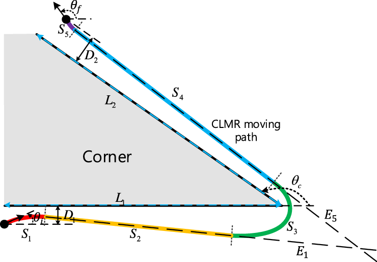
The corner environment is shown in Fig. 2. Two connected roads meet at angle $\theta_{c}$ . The width and length of the first and second roads are, respectively, $D_{1}$ and $L_{1}$ and $D_{2}$ and $L_{2}$ . The corner area is defined as $C_{a}$ . The initial and final states are given as $\mathbf{z}_{i}=[x_{i} \: y_{i} \: \theta_{i} \: \delta_{i} \: v_{i} \: \omega_{i}]^{T}$ and $\mathbf{z}_{f}=[x_{f} \: y_{f} \: \theta_{f} \: \delta_{f} \: v_{f} \: \omega_{f}]^{T}$ . At the initial state, we assume that CLMR is stopped with a zero steering angle and that it is at the origin. We obtain $\mathbf{z}_{i}$ as $[0 \: 0 \: \theta_{i} \: 0 \: 0 \: 0]^{T}$ and $\mathbf{z}_{f}$ as $[L_{1}+L_{2}\cos(\theta_c)+D_{2}\sin(\theta_c) \: D_{1}+L_{2}\sin(\theta_c)-D_{2}\cos(\theta_c) \: \theta_{f} \: 0 \: 0 \: 0]^{T}$ .

Figure 2.

Corner environment and a cornering path.

2.2. Constraints

The CLMRs use DC motors as actuators, and they are driven by an H-bridge power switching circuit with a duty ratio of the PWM; this is bounded according to

(1) \begin{equation} |u^{d}|\leq u^{d}_{\max},\ |u^{s}|\leq u^{s}_{\max},\end{equation}

where $u^{d}/u^{s}$ denote the driving/steering PWM signal and $u^{d}_{\max}/u^{s}_{\max}$ represent the maximum driving/steering PWM signal bounds. The maximum PWM signal is bounded for safety, and it cannot exceed 1 because of the limited performance of the H-bridge power switching circuit.

In a DC motor, there is a limit to the current of the actuator. Further, the generated torque is bounded to consider safety and mechanical durability. This is expressed as:

(2) \begin{equation} |\tau^{d}_{g}|\leq \tau^{d}_{\max},\ |\tau^{s}_{g}|\leq \tau^{s}_{\max},\end{equation}

where $\tau^{d}_{g}/\tau^{s}_{g}$ and $\tau^{d}_{\max}/\tau^{s}_{\max}$ denote the driving/steering generated torque and the maximum driving/steering torque bound, respectively.

In the Ackermann steering system, $\delta$ is bounded because of the mechanical structure according to

(3) \begin{equation} |\delta|\leq \delta_{\max},\end{equation}

where $\delta_{\max}$ represents the maximum steering angle.

For collision-free, there is no overlap between R(t) and $C_a$ at any time:

(4) \begin{equation} C_{a} \cap R(t) = \emptyset \:\: \text{in} \: \forall t.\end{equation}

2.3. Problem formulation

TOCTP-CLMR Problem: The cornering environment is shown in Fig. 2, and we obtain the time-optimal collision-free cornering trajectory from $\mathbf{z}_{i}$ to $\mathbf{z}_{f}$ using a dynamics model considering the PWM, torque, and steering angle constraints.

3.1. Lagrangian dynamics

We can obtain the kinematics equation and velocity constraints assuming nonslip motion [Reference Choset, Lynch, Hutchinson, Kantor, Burgard and Kavraki5]. Since CLMR move slowly, this assumption is considerably reasonable. According to Okyuama [Reference Okuyama, Maximo and Afonso38] and Kim [Reference Kim and Kim40], to avoid side slip, the lateral force should be lower than the maximum static friction force. For example, HS-589, in Appendix A.5, has the theoretical maximum translation velocity of $1.9\ \mathrm{m/s}$ (with zero steering angle), and the theoretical maximum orientation angular velocity of $2.25 \mathrm{rad}/\mathrm{s}$ with $\delta=0.25\pi \mathrm{rad}$ . In this case, the lateral force generated during rotation with the theoretical maximum translation velocity and theoretical maximum orientation angular velocity is ${\sim}430\ \mathrm{N}$ . The maximum static friction coefficient between the tire and the ground for the normal road condition is larger than 0.55 according to Wong [Reference Wong43]; therefore, the maximum static friction force is about 540 N. Hence, if HS-589 moves on the normal road except under snow or ice conditions, the nonslip assumption is acceptable. Using the Jacobian matrix $\mathbf{J}$ , we obtain the kinematic equation as:

(5) \begin{equation} \dot{\mathbf{q}}=\mathbf{J}(\mathbf{q})\mathbf{v},\end{equation}

where $\mathbf{q}$ represents the generalized coordinate vector and $\mathbf{v}$ denotes the actuator velocity vector.

Based on Eq. (5), we obtain the velocity constraints as:

(6) \begin{equation} \mathbf{A(q)}\dot{\mathbf{q}}=\mathbf{0}.\end{equation}

Note that $\mathbf{J(q)}$ denotes the null space of $\mathbf{A(q)}$ satisfying $\mathbf{A(q)J(q)}=\mathbf{0}$ and $\mathbf{J^{T}(q)A^{T}(q)}=\mathbf{0}$ . Appendix A.1 explains this is greater detail.

The dynamic equation with the torque input is given as:

(7) \begin{equation} \mathbf{M(q)}\ddot{\mathbf{q}} + \mathbf{V(q,}\dot{\mathbf{q}}) = \mathbf{B}\boldsymbol{\tau} - \mathbf{A^{T}(q)}\boldsymbol{\lambda},\end{equation}

where $\mathbf{M(q)}$ , $\mathbf{V(q},\dot{\mathbf{q}})$ , $\mathbf{B}$ , $\boldsymbol{\tau}$ , and $\boldsymbol{\lambda}$ denote the inertia matrix, centripetal and Coriolis force matrix, input transformation matrix, torque input, and Lagrangian multiplier, respectively. For CLMRs, we can represent $\mathbf{q}$ and $\dot{\mathbf{q}}$ as a function of $\mathbf{z}$ . Appendix 7.2 details this process.

3.2. DC motor actuator dynamics

Since the battery power of MR is limited, using the full resource of the actuator of MR is important to ensure time optimality. Therefore, including the DC motor actuator dynamics is more suitable than considering only the torque bounds for time optimality. Because the electrical time constant of the DC motor is considerably lower than the mechanical time constant, we can neglect the inductance and devise the electrical equation as:

(8) \begin{equation} V_{s}\mathbf{u} = \mathbf{R_{a}}\mathbf{i} + \mathbf{K_{b}}\mathbf{v}, \boldsymbol{\tau_{g}}=\mathbf{K_{t}}\mathbf{i}\end{equation}

where $V_{s}$ , $\mathbf{u}$ , $\mathbf{R_{a}}$ , $\mathbf{i}$ , $\mathbf{K_{b}}$ , $\mathbf{K_{t}}$ , and $\boldsymbol{\tau_{g}}$ denote the supply voltage, PWM motor control signal vector, armature resistance matrix, armature current vector, back-emf constant matrix, torque constant matrix, and generated torque vector, respectively.

Using $\mathbf{K_{t}}$ , we can rewrite Eq. (2) as the current constraints, as shown below:

(9) \begin{equation} |i^{d}|\leq i^{d}_{\max},\ |i^{s}|\leq i^{s}_{\max}.\end{equation}

Here, $i^{d}/i^{s}$ denotes the driving/steering armature current and $i^{d}_{\max}/i^{s}_{\max}$ is the maximum driving/steering current bound. More details are provided in Appendix A.3.

3.3. Dynamic model for CLMRs

We obtain the torque equation, including the friction torque and steering braking torque as:

(10) \begin{equation} \boldsymbol{\tau}=\boldsymbol{\tau_{g}} - \boldsymbol{\tau_{f}} - \boldsymbol{\tau_{b}},\end{equation}

where $\boldsymbol{\tau_{f}}$ denotes the friction torque vector and $\boldsymbol{\tau_{b}}$ denotes the steering braking torque vector. Among various types of friction [Reference Armstrong-Hélouvry, Dupont and de Wit41], we consider the two most dominant frictions forms Coulomb and viscous friction as:

(11) \begin{equation} \boldsymbol{\tau_{f}}=\mathbf{F_{v}}\mathbf{v} + \mathbf{F_{c}}\mathbf{v_{sign}},\end{equation}

where $\mathbf{F_{v}}$ denotes the viscous friction matrix and $\mathbf{F_{c}}$ denotes the Coulomb friction matrix. Appendix A.4 contains additional details. According to Eqs. (8)–(11), when we apply step PWM signal to the motor while the robot is stopped, the current has an instantaneous high value when the robot starts to move and it starts to decreases exponentially after that; finally, it reaches the steady state with a constant current value.

In CLMRs, the lateral force of the front steering wheel is not always orthogonal to the moving direction of the CLMR, and this causes steering braking. As the steering angle increases, the steering braking torque also increases, which interferes with the driving. Under nonslip motion, the steering braking torque caused by the lateral force of the front steering wheel is expressed as:

(12) \begin{equation} \boldsymbol{\tau_{b}}=[C_{b}\tan^{2}(\delta)(\dot{\phi^{d}})^{2} \:\: 0]^{T},\end{equation}

where $C_{b}$ denotes the steering braking coefficient. Appendix A.4 presents this in more detail.

Finally, we can obtain the dynamic model for CLMRs. First, we eliminate the Lagrange multiplier in Eq. (7) as:

(13) \begin{equation} \mathbf{J^{T}(z)}\mathbf{M(z)}\ddot{\mathbf{q}} + \mathbf{J^{T}(z)}\mathbf{V(z)} =\mathbf{J^{T}(z)}\mathbf{B}\boldsymbol{\tau}.\end{equation}

Using Eqs. (5)–(13), we obtain the relationship between $\dot{\mathbf{v}}$ and $\mathbf{u}$ as:

(14) \begin{equation} \dot{\mathbf{v}}= \bar{\mathbf{M}}^{\mathbf{-1}}_{\mathbf{1}}\mathbf{(z)} ( ( -\bar{\mathbf{M}}_{\mathbf{2}}\mathbf{(z)} - \mathbf{R^{-1}_{a}}\mathbf{K_{t}}\mathbf{K_{b}} - \mathbf{F_{v}})\mathbf{v} -\bar{\mathbf{V}}\mathbf{(z)} - \mathbf{F_{c}}\mathbf{v}_{sign}-\boldsymbol{\tau_{b}}\mathbf{(z)} + V_{s}\mathbf{R^{-1}_{a}}\mathbf{K_{t}}\mathbf{u}).\end{equation}

where $\bar{\mathbf{M}}_{\mathbf{1}}\mathbf{(z)}=\mathbf{J^{T}(z)M(z)J(z)}$ , $\bar{\mathbf{M}}_{\mathbf{2}}\mathbf{(z)}=\mathbf{J^{T}(z)M(z)}\dot{\mathbf{J}}\mathbf{(z)}$ , $\bar{\mathbf{V}}\mathbf{(z)}=\mathbf{J^T(z)V(z)}$ , and $\mathbf{J^T(z)B(z)}=\mathbf{I_{2}}$ .

Letting $\mathbf{p}=[x \quad y \quad \theta \quad \delta]^{T}$ be the pose vector, we obtain $\mathbf{p}$ from $\mathbf{v}$ as:

(15) \begin{equation} \dot{\mathbf{p}}=\bar{\mathbf{J}}\mathbf{(z)v}, \bar{\mathbf{J}}\mathbf{(z)}= \begin{bmatrix} r\cos\theta & \quad r\sin\theta & \quad r\tan\theta/l & \quad 0 & \quad 0 & \quad 0 \\[5pt] 1 & \quad 1 & \quad 1 & \quad 1 & \quad 0 & \quad 0 \end{bmatrix}^{T}.\end{equation}

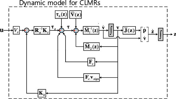
The state vector $\mathbf{z}$ can be expressed as $\mathbf{z}=[\mathbf{p^{T}}$ $\mathbf{v^{T}}$ ], and the block diagram of the CLMR dynamics is shown in Fig. 3.

Figure 3.

The Block diagram of the CLMR dynamic model.

4.1. TOCTP-CLMR problem with dynamic model

Considering model and constraints, we can rewrite the TOCTP-CLMR problem as:

\begin{gather*} \textbf{minimize} \:\: t_{f} \\[3pt] \textbf{Subject to} \\[3pt] \dot{\mathbf{v}}= \bar{\mathbf{M}}^{\mathbf{-1}}_{\mathbf{1}}\mathbf{(z)} ( (-\bar{\mathbf{M}}_{\mathbf{2}}\mathbf{(z)} - \mathbf{R^{-1}_{a}}\mathbf{K_{t}}\mathbf{K_{b}} - \mathbf{F_{v}})\mathbf{v} \\[3pt] -\bar{\mathbf{V}}\mathbf{(z)} - \mathbf{F_{c}}\mathbf{v}_{sign}-\boldsymbol{\tau_{b}}\mathbf{(z)} + V_{s}\mathbf{R^{-1}_{a}}\mathbf{K_{t}}\mathbf{u}), \\[3pt] \dot{\mathbf{p}} = \bar{\mathbf{J}}\mathbf{(z)v}, \: \mathbf{z}=[\mathbf{p^{T}} \mathbf{v^{T}}], \\[3pt] \mathbf{z}(\text{0})=\mathbf{z}_{i}, \: \mathbf{z} (\text{$t_{f}$})=\mathbf{z}_{f}, \\[3pt] |u^{d}(\text{t})| \leq u^{d}_{\max}, \: |u^{s}(\text{t})| \leq u^{s}_{\max},\: \text{t} \in \text{[0 $t_{f}$]}, \\ \end{gather*}

\begin{gather*} |i^{d}(\text{t})| \leq i^{d}_{\max}, \: |i^{s}(\text{t})| \leq i^{s}_{\max},\: \text{t} \in \text{[0 $t_{f}$]}, \\[3pt] |\delta(t)| \leq \delta_{\max}, \: t \in \text{[0 $t_{f}$]}, \\[3pt] C_{a} \cap R(t) = \emptyset, \: t \in \text{[0 $t_{f}$]},\end{gather*}

where $t_{f}$ denotes the total time required to pass the corner.

4.2. Approach

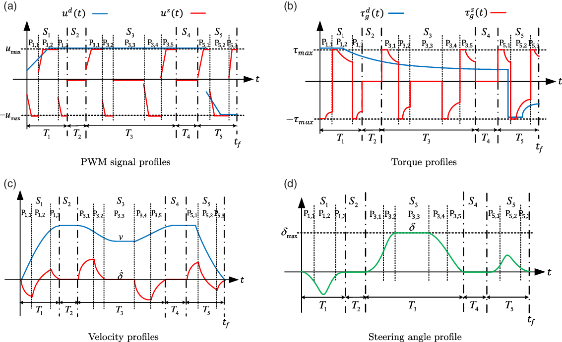
For realizing time optimality, we divide the cornering trajectory into five sections as shown in Fig. 2. The corresponding inputs, torques (or currents), and velocities are depicted in Fig. 4. Three rotational sections are considered: $S_{1}$ denotes the initial rotational section, $S_{3}$ represents the middle rotational section, and $S_{5}$ represents the final rotational section. Two translational sections, $S_{2}$ and $S_{4}$ , connect to the rotational sections. In addition, the time duration of each section $S_{n}$ is given as $T_{n}$ ( $n=1,2,3,4,5$ ). This is similar to the human driving behavior and the concept of Dubins path [Reference Dubins13]. The use of fewer sections leads to increased traveled distance; then, adding more section is useless for the traveled distance and time optimality.

Figure 4.

Example profiles of the optimal trajectory. (a) PWM signal profiles with PWM bounds. (b) Generated torque profiles with the torque bounds. (c) Translational and steering angular velocity profiles. (d) Steering angle with maximum steering angle.

For time optimality, the translational velocity should be maximized so that the driving PWM signal and current (or torque) satisfy the bang-bang [Reference Bryson and Ho42] principle as shown in Fig. 4(a) and (b), respectively. Hence, there are two driving PWM intervals, and each PWM interval is divided into a pre-varying PWM signal duration and a post-constant PWM signal duration. In a pre-varying PWM signal duration, the PWM signal varies to satisfy the torque constraint while not exceeding the maximum PWM bound. After the pre-varying PWM signal duration, the PWM signal has constant maximum PWM value in the post-constant PWM signal duration. If the torque constraint is too large and unactivated, the pre-varying PWM signal duration may not achieved.

For time optimality in each rotational section, we select the minimum turning radius and refer to the QSR. Similar to the driving PWM signal, we satisfy the bang-bang principle for the PWM, current(=torque), and steering angle constraint in the steering PWM signal as shown Fig. 4(a), (b), and (d). In QSR, $S_{n}$ contains three or five steering PWM signal intervals ( $P_{i,n}$ ) according to the required rotation angle. In a small rotation (that required q small orientation angle variation) motion, there are three $P_{i,n}$ ( $i=1,2,3$ ) as depicted for $S_{1}$ and $S_{5}$ in Fig. 4, because the maximum steering angle constraint is not activated as shown in Fig. 4(d). In cases with large rotations (requiring large orientation angle variation), there are five $P_{i,n}$ ( $i=1,2,3,4,5$ ) as shown in the relation to $S_{3}$ in Fig. 4. In such a case, it becomes necessary to consider the maximum steering angle constraint. Accordingly, $\delta$ is increased from 0 to $\delta_{\max}$ for $P_{1,n}$ and $P_{2,n}$ . Then it is kept constant at $\delta_{\max}$ with the arc in $P_{3,n}$ . Finally, the steering angle decreases to 0 for $P_{4,n}$ and $P_{5,n}$ in Fig. 4(d). For each $P_{i,n}$ , the time duration is given as $T_{i,n}$ and it is composed of the pre-varying PWM signal and the post-constant PWM signal duration to satisfy the current(or torque) and the PWM input constraints that are similar to the driving PWM signal.

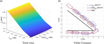
By examining $t_{f}$ according to $u^{s}(t)$ and $\tau_{g}^{s}(t)$ during the rotation transition and $\delta(t)$ in the arc interval, we find that QSR leads to time optimality in Fig. 5(a). $Input_{tra}$ refers to the ratio of the maximum steering PWM signal excluding the arc interval, and $\delta_{arc}$ refers to the steering angle in the arc interval. In this figure, we obtain $t_{f}$ varying $Input_{tra}$ and $\delta_{arc}$ , and we see that using the maximum $Input_{tra}$ ( $Input_{tra}$ ratio = 1) and the maximum $\delta_{arc}$ ( $\delta_{arc}$ ratio = 1) in the rotation leads time-optimal solution. In addition, we noted that QSR ( $Input_{tra}$ ratio=1 and $\delta_{arc}$ ratio=1) has the minimum $t_{f}$ , as shown in Fig. 5(a). Further, it has the minimum turning radius because of using the maximum steering angle in the arc interval with the maximum transition input. Further, it has the minimum travel distance, as shown in Fig. 5(b).

Figure 5.

Simulation result with respect to $\delta_{arc}$ and $Input_{tra}$ : (a) corner passing time, (b) paths for three cases: red (QSR case), black ( $\delta_{arc}$ /0.7 $Input_{tra}$ , and blue (0.7 $\delta_{arc}/Input_{tra}$ ).

There are two reasons why QSR is time-optimal: (1) travel distance and (2) maintaining high speed. By using the maximum input of the steering in the rotation motion, QSR maximizes the orientation angular velocity and thus reduces the turning radius and turning time. With the use of the minimum turning radius, as shown in Fig. 5(b), QSR has the shortest trajectory similar to in-course cornering during speed skating. For the time-optimal trajectory, it is necessary to increase speed and reduce the traveled distance. With QSR, we can use the smallest turning radius, and this leads to the shortest traveled distance. In addition, the shortest turning time of QSR reduces the steering braking effect that disturbs the speed and decreases ratio of rotation motion that leads to a high average speed. Hence, QSR simultaneously achieves the shortest traveled distance and high speed.

4.3. Algorithm

The overall TOCTP-CLMR algorithm is represented as Algorithm 1 and shown in Fig. 6. In the TOCTP-CLMR, we adjust $\Delta\theta_{1}$ (the amount of orientation angle change in $S_{1}$ ) and $\Delta\theta_{5}$ (the amount of orientation angle change in $S_{2}$ ) to obtain the time-optimal collision-free trajectory. For computational efficiency, $S_{3}$ is planned by assuming the initial condition, and we vary this assumed initial condition for the continuous velocity. We can plan the rotational sections independently. Then, we plan the translational sections to connect the rotational sections easily. In each rotational section, we use the QSR section planning (QSRP) sub-algorithm, presented here as Algorithm 2.

Figure 6.

Algorithm flow for the TOCTP-CLMR.

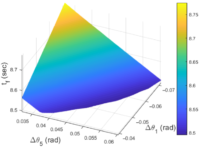
We used 2D optimization method to obtain the optimal value of $\Delta\theta_{1}$ and $\Delta\theta_{5}$ . We find that a trend of $t_{f}$ against $\Delta\theta_{1}$ and $\Delta\theta_{5}$ has a convex form and it is bounded because of a collision, as shown in Fig. 7. If we increase $\Delta\theta_{1}$ or $\Delta\theta_{5}$ , the traveling distance increases, and the time optimality is lost. If we decrease these values, we can reduce the distance traveled; however, this can cause a collision because the path is too close to the corner. Accordingly, we attempt to find the time-optimal and collision-free $\Delta\theta_{1}$ and $\Delta\theta_{5}$ .

Figure 7.

Trend of $t_{f}$ with respect to $\Delta\theta_{1}$ and $\Delta\theta_{5}$ .

When $\Delta\theta_{1}$ and $\Delta\theta_{5}$ are given, we can obtain the continuous velocity and path trajectory using QSRP. In QSRP, the rotational section can be planned when the rotation angle and the initial state are given. For computational efficiency, we isolated each rotational section using the assumed initial state of $S_{3}$ . First, we plan $S_{1}$ with the initial state and $\Delta\theta_{1}$ and then, we obtain the final state of $S_{1}$ to obtain $E_{1}$ (the extension line of the final state of $S_{1}$ ). For $S_{5}$ , we plan $S_{5}$ using QSRP in a reverse time order because the final state and $\Delta\theta_{5}$ are given; then, we obtain the initial state of $S_{5}$ and $E_{5}$ (the extension line of the initial state of $S_{5}$ ). In section $S^{\prime}_{3}$ , the orientation angle change is given as the remaining rotational angle and the initial state can be obtained through $v_{3}^{i}$ and the zero initial pose. After planning $S^{\prime}_{3}$ , we shift $S^{\prime}_{3}$ to fit $E_{1}$ and $E_{5}$ as shown in Fig. 2 for the continuous path, and then, we obtain $S_{3}$ . After planning the rotation sections, we plan the translational sections to connect the rotational sections. The path is continuous; however, the velocity cannot guarantee continuity. Therefore, we vary $v_{3}^{i}$ to ensure that the final velocity of $S_{2}$ is equal to $v_{3}^{i}$ for the continuous velocity. Through the above series of processes, we obtain an overall trajectory that is a continuous path and velocity correspondingly by $\Delta\theta_{1}$ and $\Delta\theta_{5}$ .

In QSRP, we plan the rotational section $S_{n}$ with the given initial state, $\Delta\theta_{n}$ and the driving input as shown in Algorithm 2. We plan $S_{n}$ so that the noninclusion of the arc interval that $S_{n}$ is divided into the three intervals, as shown in $S_{1}$ and $S_{5}$ in Fig. 4. In this case, each steering torque input of the pre-varying PWM signal duration is determined via

(16) \begin{equation} \tau^{s}_{n,1}=\tau^{s}_{n,3}=sign(\Delta\theta_{n})\tau^{s}_{\max}, \: \tau^{s}_{n,2}=-sign(\Delta\theta_{n})\tau^{s}_{\max}.\end{equation}

We can convert to these constant torque inputs to vary the PWM input profile using the dynamic model, as shown in Fig. 4(a). After the pre-varying PWM signal duration, we plan the post-constant PWM signal duration given as:

(17) \begin{equation} u^{s}_{n,1}=u^{s}_{n,3}=sign(\Delta\theta_{n})u^{s}_{\max}, \: u^{s}_{n,2}=-sign(\Delta\theta_{n})u^{s}_{\max}.\end{equation}

Then, the time duration of each interval can be determined to satisfy the final condition which is given as:

(18) \begin{equation} \delta_{n,3}=\delta_{n}^{f}=0, \: \dot{\delta_{n,3}}=\dot{\delta_{n}^{f}}=0, \: \theta_{n,3}=\theta_{n}^{f}=\theta_{n}^{i}+\Delta\theta_{n}, \:\end{equation}

using a 3D search method.

Next, QSRP checks whether the planned $S_{n}$ meets the maximum steering constraint. If so we return $S_{n}$ and finish; if not, an arc interval is required. Therefore, we re-plan $S_{n}$ with the arc interval that $S_{n}$ is divided into five intervals as $S_{3}$ in Fig. 4. Each steering torque input of the pre-varying PWM signal duration is determined as:

(19) \begin{equation} \tau^{s}_{n,1}=\tau^{s}_{n,4}=sign(\Delta\theta_{n})\tau^{s}_{\max}, \: \tau^{s}_{n,2}=\tau^{s}_{n,5}=-sign(\Delta\theta_{n})\tau^{s}_{\max}, \: \tau^{s}_{n,3}=0.\end{equation}

Further, We can convert these torque inputs into varying PWM input signals by using the dynamic model. The post-constant PWM signal duration of each interval is given as:

(20) \begin{equation} u^{s}_{n,1}=u^{s}_{n,4}=sign(\Delta\theta_{n})u^{s}_{\max}, \: u^{s}_{n,2}=u^{s}_{n,5}=-sign(\Delta\theta_{n})u^{s}_{\max}, \: u^{s}_{n,3}=0.\end{equation}

In the arc interval, the zero PWM input signal exists to maintain the maximum steering angle. Then, QSRP finds the time duration of the first and second intervals for the initial state of the arc interval; the conditions are given as:

(21) \begin{equation} \delta_{n,2}=\delta_{\max}, \: \dot{\delta_{n,2}}=0, \:\end{equation}

using a 2D search method. Next, QSRP finds the time duration of the third, fourth, and fifth interval for the final state. These are given as:

(22) \begin{equation} \delta_{n,5}=\delta_{n}^{f}=0, \: \dot{\delta_{n,5}}=\dot{\delta_{n}^{f}}=0, \: \theta_{n,5}=\theta_{n}^{f}=\theta_{n}^{i}+\Delta\theta_{n}. \:\end{equation}

5.1. Simulation

We conducted a simulation to demonstrate the validity of the TOCTP-CLMR algorithm. The target CLMR is the HS-589 model (see Appendix A). Further the corner environment is given as $L_{1} = 5$ m, $L_{2}=7$ m, $D_{1}=0.4$ m, $D_{2}=1$ m, and $\theta_{c}=0.75\pi \mathrm{rad}$ , as shown in Fig. 2. The initial and final orientation angle are correspondingly $\theta^{i}=0 \mathrm{rad}$ and $\theta^{f}=\theta_{c}$ . We added the following margins to PWM bounds as $u^{d}_{\max}=u^{s}_{\max}=0.75$ , and we set the torque bound for safety as $\tau^{d}_{\max}=50$ N (include gear) and $\tau^{s}_{\max}=70$ N (include gear). The steering angle constraint was given as $\delta_{\max}=0.25\pi \mathrm{rad}$ . The optimal trajectory had values of $\Delta\theta_{1}=-0.0545\ \mathrm{rad}$ , $\Delta\theta_{5}=0.0498\ \mathrm{rad}$ , and $t_{f}=8.5069$ s.

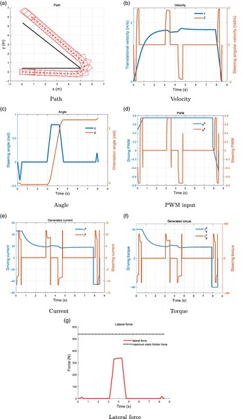
We plot the lateral force and maximum static friction force when the maximum static friction coefficient is 0.55 in Fig. 8(g). To verify the nonslip motion assumption, we check the lateral force is lower than the maximum static friction force [Reference Okuyama, Maximo and Afonso38, Reference Kim and Kim40]. If this condition is not satisfied, then the side slip is not negligible. Since the lateral force in this case was always lower than the maximum static friction force (540 N), the nonslip motion assumption was reasonable. Figure 8(a) indicates that the CLMR traverses the corner without a collision to the final pose. Because $D_{1}$ is too narrow, we find that the CLMR turns right at $S_{1}$ to avoid collision. Figure 8(b) shows that the velocity decreases at $S_{3}$ because of steering braking. As shown in Fig. 8(c), the trajectory satisfies the final orientation and steering angle, and the steering angle does not exceed the maximum steering angle constraint. PWM input profiles are shown in Fig. 8(d), the generated torques are given in Fig. 8(f), and the current of motors are presented in Fig. 8(e). Besides the steering input in the arc interval, we find the pre-varying PWM signal duration. The generated torque (or motor current) profiles satisfy the torque (or current) constraints and the CLMR uses the maximum torque at the pre-varying PWM signal duration of every motion and satisfies the bang-bang principle. Further, in Fig. 8(d), the PWM input profiles satisfy the maximum PWM input constraints. In each post-constant PWM signal duration, the PWM input profile uses the maximum value for the bang-bang principle. By providing the bang-bang inputs (including the torque and PWM) to the actuator motors, the TOCTP-CLMR can obtain a time-optimal trajectory, which validates the algorithm.

Figure 8.

Simulation result. There are simulation paths, steering angles, orientation angles, PWM input signals, currents, torques, and lateral force.

5.2. Experiment

We performed open-loop step response experiments to validate the proposed dynamic model. The first-order exponential responses with the step PWM signal are shown in Figs. 9 and 10. There are small jitters in each case; however, these experiment responses are similar to the simulation results. In the current experiments shown in Figs. 9(b) and 10(b), the current hits a peak and then decreases exponentially to reach the steady state. In the steady state, the current is maintained as a constant. The differences between the simulation result and the experiment result are that there is a ripple in the experiment caused by measurement noise that does not exist in the simulation result, and the slope of the current for this experiment is lower than that for the simulation because of the inductance of the motor that disturbs current distribution. However, the shape and tendency of the simulation and the experiment are similar.

Figure 9.

Open-loop driving experiments with step input $u^d=0.6$ after 1 s.

Figure 10.

Open-loop steering experiments with step input $u^s=0.3$ after 1 s.

When varying the steering angle, we conducted an experiment about the steering braking torque. In Fig. 11(a), we plot three cases of the steering angle: $0 \mathrm{rad}$ (blue), $0.66 \mathrm{rad}$ (red), and $0.89 \mathrm{rad}$ (black). Although the three profiles have the same step driving PWM input, the steady-state velocities are different. In Fig. 11(b), we plot the steady-state velocities with respect to the steering angle, and the difference is as high as 5%; this is not negligible with regard to time optimality. We converted these steady-state velocities into the steering braking torque, in Fig. 11(c), and we plotted the experimental result of $\tau_{b}$ (red) and those of the simulation using the proposed model (blue). Because the experimental and simulation results are similar, we successfully demonstrate the validity of the proposed dynamic model.

Figure 11.

Steering braking torque experiments.

Based on the proposed dynamic model, we designed the trajectory tracking controller using the resolved motion acceleration control for a trajectory tracking experiment. Because the resolved motion acceleration controller uses not only the desired position but also the desired acceleration, it is an appropriate dynamic model that includes actuator dynamics. A block diagram of the controller is shown in Fig. 12, where $\mathbf{p}_{d}$ , $\mathbf{v}_{d}$ , and $\mathbf{z}_{d}$ are the desired pose, actuator velocity, and state vector, respectively. We added feedback with $\mathbf{K}_{p}$ (the position error feedback gain matrix) and $\mathbf{K}_{v}$ (the velocity error feedback gain matrix) to compensate for any unexpected errors in the velocity and pose. In the inverse dynamic model, we use the pseudo-inverse matrix of $\mathbf{J}^{\#}=(\mathbf{J}^{T}\mathbf{J})^{-1}\mathbf{J}^{T}$ instead of $\mathbf{J}^{-1}$ , given that $\mathbf{J}^{-1}$ does not exist,.

Figure 12.

Resolved acceleration controller for CLMR.

We conducted a trajectory tracking experiment to validate the time-optimal trajectory of the TOCTP-CLMR. To ensure a trackable trajectory, we set conservative bounds on the PWM signals and $\delta_{\max}$ in the desired trajectory. The desired trajectory is the time-optimal trajectory of the TOCTP-CLMR, as shown in Fig. 13.

Figure 13.

Trajectory tracking experiments. HS-589 tracks the trajectory given as Fig. 8 with the resolved acceleration controller as Fig. 12.

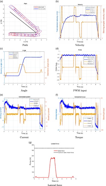
In Fig. 13(g), we see that the lateral force is always lower than the maximum static friction force. In the experiment trajectory, the maximum lateral force is about 370 N and it is lower than the maximum static friction force (540 N) when the maximum static friction coefficient is 0.55. Therefore, no slip occurs in the experiment. In addition, we can analyze how slip occurs. In this case, the normal force exerted by each wheel was 245 N, with the maximum lateral force of each wheel being 92.5 N. The tire cornering stiffness is approximately 222.5 N/degree in the tire model of vehicle simulation [Reference Wade Allen, Rosenthal, Klyde and Chrstos44]. Hence, the maximum slip angle was given as 0.42 degree, which was negligible.

The desired and actual paths are shown in Fig. 13(a). The CLMR tracks quite well without colliding; at the final point, there is a position error of $0.08$ m, while the CLMR moves approximately 12 m. The translational and steering angular velocity profiles of the desired and actual trajectory are similar, as shown in Fig. 13(b). The steering and orientation angle profiles are plotted in Fig. 13(c), and they show the corresponding final errors of only $0.009\ \mathrm{rad}$ in $\theta$ and 0 rad in $\delta$ . In Fig. 13(d), we plot $\mathbf{u}$ from the experiment and simulation, and we find that they are similar; $\mathbf{u}$ in the experiment shows a ripple to compensate for errors; however, it is close to that in the simulation on average. For the generated current and torque, they are plotted in Figs. 13(e) and (f). Because we ignore the inductance of the actuator, experimental results change more slowly than the simulation results. Nevertheless, when viewed as a whole, there is a similar trend. Hence, the experimental result demonstrates the feasibility of the result time-optimal trajectory from the TOCTP-CLMR, thus also demonstrating the validity of the TOCTP-CLMR.