1. Introduction
Dirac (Reference Dirac1928) derived a relativistic covariant representation of the Schrodinger equation with positive-definite probability density by, in essence, taking the square root of the Klein–Gordon wave equation. With the introduction of Dirac spinors, there were immediate attempts to connect Maxwell's equations with the Dirac equation (Laporte & Uhlenbeck Reference Laporte and Uhlenbeck1931; Oppenheimer Reference Oppenheimer1931; Moses Reference Moses1959), particularly with the introduction of the Riemann–Silberstein (RS) vector (Bialynicki-Birula Reference Bialynicki-Birula1996; Coffey Reference Coffey2008) for the electromagnetic field. More recent attempts have further coupled the Maxwell equations to various field theories (Yepez Reference Yepez2002, Reference Yepez2005, Reference Yepez2016; Kulyabov, Kolokova & Sevatianov Reference Kulyabov, Kolokova and Sevatianov2017; Jestadt et al. Reference Jestadt, Ruggenthaler, Oliveira, Rubio and Appel2018).
Here we give an explicit unitary quantum lattice algorithm (QLA) for Maxwell equations in material media, building on our earlier QLA for solitons (Vahala, Vahala & Yepez Reference Vahala, Vahala and Yepez2003a,Reference Vahala, Vahala and Yepezb, Reference Vahala, Vahala and Yepez2004, Reference Vahala, Vahala and Yepez2005; Oganesov et al. Reference Oganesov, Vahala, Vahala, Yepez and Soe2016a,Reference Oganesov, Flint, Vahala, Vahala, Yepez and Soeb, Reference Oganesov, Vahala, Vahala and Soe2018) and Bose–Einstein condensates (Yepez, Vahala & Vahala Reference Yepez, Vahala and Vahala2009a; Yepez et al. Reference Yepez, Vahala, Vahala and Soe2009b; Vahala et al. Reference Vahala, Yepez, Vahala, Soe, Zhang and Ziegeler2011, Reference Vahala, Yepez, Vahala and Soe2012a,Reference Vahala, Zhang, Yepez, Vahala and Soeb, Reference Vahala, Soe, Vahala and Yepez2019a,Reference Vahala, Vahala, Soe, Ram and Yepezb, Reference Vahala, Vahala, Soe and Ram2020c; Vahala, Soe & Vahala, Reference Vahala, Soe and Vahala2020a,Reference Vahala, Vahala and Soeb). QLAs are of much interest because their interleaved sequence of unitary collision and streaming operators can be immediately modelled by qubit gates. This permits immediate encoding onto a quantum computer. An interesting by-product of QLA is that these algorithms are also ideally parallelizable on classical supercomputers and typically lead to algorithms that can outperform standard classical algorithms in parallelization and numerical stability.
Consider Maxwell equations (in standard notation)
 \begin{equation}\left.\begin{gathered} {\boldsymbol{\nabla}\boldsymbol{\cdot}\boldsymbol{D}(\boldsymbol{x},t) = \rho (\boldsymbol{x},t),\quad \boldsymbol{\nabla}\boldsymbol{\cdot }\boldsymbol{B}(\boldsymbol{x},t) = 0}\\ {\boldsymbol{\nabla} \times \boldsymbol{H}(\boldsymbol{x},t) = \boldsymbol{J}(\boldsymbol{x},t) + \dfrac{{\partial \boldsymbol{D}(\boldsymbol{x},t)}}{{\partial t}},\quad \boldsymbol{\nabla} \times \boldsymbol{E}(\boldsymbol{x},t) = -\dfrac{{\partial \boldsymbol{B}(\boldsymbol{x},t)}}{{\partial t}}} \end{gathered}\right\},\end{equation}
where the external charge and current densities are  $\rho $ and J. For linear isotropic material media, the electromagnetic fields obey the constitutive equations
 \begin{equation}\boldsymbol{D}(\boldsymbol{x},t) = \varepsilon (\boldsymbol{x},t)\boldsymbol{E}(\boldsymbol{x},t),\quad \boldsymbol{B}(\boldsymbol{x},t) = \mu (\boldsymbol{x},t)\boldsymbol{H}(\boldsymbol{x},t),\end{equation}
where the permittivity  $\varepsilon (\boldsymbol{x},t) = {\varepsilon _0}{\varepsilon _r}(\boldsymbol{x},t)$ and the permeability
 $\mu (\boldsymbol{x},t) = {\mu _0}{\mu _r}(\boldsymbol{x},t)$. (The speed of light in a vacuum
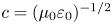 $c = {({\mu _0}{\varepsilon _0})^{ - 1/2}}$.) To rewrite the Maxwell equations into matrix form illustrative of the Dirac equation, it is convenient to introduce the two RS vectors (Bialynicki-Birula Reference Bialynicki-Birula1996; Khan Reference Khan2005; Jestadt et al. Reference Jestadt, Ruggenthaler, Oliveira, Rubio and Appel2018)
 \begin{equation}{\boldsymbol{F}^ \pm } = \frac{1}{{\sqrt 2 }}\left[ {\sqrt \varepsilon \boldsymbol{E} \pm i\frac{\boldsymbol{B}}{{\sqrt \mu }}} \right],\end{equation}
for the two polarizations of the electromagnetic fields. In homogeneous media, there is no mixing of the polarizations, so the RS vectors remain uncoupled. In inhomogeneous media, there is coupling of the polarizations resulting in the need to use both RS vectors.
Following Khan (Reference Khan2002, Reference Khan2005), we introduce
 \begin{equation}v(\boldsymbol{x},t) = \frac{1}{{\sqrt {\varepsilon \mu } }},\quad h(\boldsymbol{x},t) = \sqrt {\frac{\mu }{\varepsilon }} ,\end{equation}
so that the Maxwell equations are (Khan Reference Khan2005)
 \begin{equation}\left. {\begin{gathered} i\dfrac{{\partial {\boldsymbol{F}^ \pm }}}{{\partial t}} = \pm v\boldsymbol{\nabla} \times {\boldsymbol{F}^ \pm } \pm \dfrac{1}{2}\boldsymbol{\nabla}v \times {\boldsymbol{F}^ \pm } \pm \dfrac{v}{{2h}}\boldsymbol{\nabla}h \times \boldsymbol{F}^{\pm}\\ \quad \qquad + \dfrac{i}{2}\left( {\dfrac{{\partial \ln v}}{{\partial t}}{\boldsymbol{F}^ \pm } + \dfrac{{\partial \ln h}}{{\partial t}}\boldsymbol{F}^{\pm}} \right) - i\sqrt {\dfrac{{vh}}{2}\boldsymbol{J}}\\ {\boldsymbol{\nabla}\boldsymbol{\cdot }{\boldsymbol{F}^ \pm } = \dfrac{1}{{2v}}\boldsymbol{\nabla}v\boldsymbol{\cdot}\boldsymbol{F}^{\pm} + \dfrac{1}{{2h}}\boldsymbol{\nabla}h\boldsymbol{\cdot}\boldsymbol{F}^{\pm} + \sqrt {\dfrac{{vh}}{2}} \rho } \end{gathered}} \right\}.\end{equation}
Polarization coupling occurs through either spatial or temporal time variations of  $h(\boldsymbol{x},t)$, (1.4a,b). In matrix form, (1.5) can be written as the time evolution of the 8-spinor components (Khan Reference Khan2005)
 \begin{align}\begin{array}{l} \dfrac{\partial }{{\partial t}}\begin{pmatrix} {\varPsi^ + }\\ {\varPsi^ - } \end{pmatrix} - \dfrac{1}{2}\dfrac{{\partial \ln v}}{{\partial t}}\begin{pmatrix} {\varPsi^ + }\\ {\varPsi^ - } \end{pmatrix} + \dfrac{{i{M_z}{\alpha _y}}}{2}\dfrac{{\partial \ln h}}{{\partial t}}\begin{pmatrix} {\varPsi^ - }\\ {\varPsi^ + } \end{pmatrix}\\ \quad = - v\begin{pmatrix} \boldsymbol{M}\boldsymbol{\cdot}\boldsymbol{\nabla} + \boldsymbol{\varSigma }\boldsymbol{\cdot}\dfrac{{\boldsymbol{\nabla}v}}{{2v}}\quad - i{M_z}\boldsymbol{\varSigma }\boldsymbol{\cdot}\dfrac{{\boldsymbol{\nabla}h}}{{2h}}{\alpha_y}\\ - i{M_z}{\boldsymbol{\varSigma }^\ast }\boldsymbol{\cdot}\dfrac{{\boldsymbol{\nabla}h}}{{2h}}{\alpha_y}\quad {\boldsymbol{M}^\ast }\boldsymbol{\cdot}\boldsymbol{\nabla} + {\boldsymbol{\varSigma }^\ast }\boldsymbol{\cdot}\dfrac{{\boldsymbol{\nabla}v}}{{2v}} \end{pmatrix}\begin{pmatrix} {\varPsi^ + }\\ {\varPsi^ - } \end{pmatrix}- \begin{pmatrix} {W^ + }\\ {W^ - } \end{pmatrix}, \end{array}\end{align}
with the Cartesian RS components and source matrices defined by
 \begin{equation}{\varPsi ^ \pm } = \begin{pmatrix} { - F_x^ \pm \pm iF_y^ \pm }\\ {F_z^ \pm }\\ {F_z^ \pm }\\ {F_x^ \pm \pm iF_y^ \pm } \end{pmatrix},\quad {W^ \pm } = \frac{1}{{\sqrt {2\varepsilon } }}\begin{pmatrix} { - {j_x} \pm i{J_y}}\\ {{J_z} - v\rho }\\ {{J_z} - v\rho }\\ {{j_x} \pm i{J_y}} \end{pmatrix}.\end{equation}
The 4 × 4 matrices M in (1.6) are just the tensor product of the Pauli spin matrices with the 2 × 2 identity matrix  ${I_2}:\boldsymbol{M}\boldsymbol{=}\boldsymbol{\sigma } \otimes {I_2}$, with
 ${M_z} = {\sigma _z} \otimes {I_2}$,
 $\boldsymbol{\sigma } = ({\sigma _x},{\sigma _y},{\sigma _z})$ and
 \begin{equation}{\sigma _x} = \begin{pmatrix} 0&1\\ 1&0 \end{pmatrix},\quad {\sigma _y} = \begin{pmatrix} 0&{ - i}\\ i&0 \end{pmatrix},\quad {\sigma _z} = \begin{pmatrix} 1&0\\ 0&{ - 1} \end{pmatrix}.\end{equation}
Finally
 \begin{equation}\boldsymbol{\alpha } = \begin{pmatrix} 0&\boldsymbol{\sigma }\\ \boldsymbol{\sigma }&0 \end{pmatrix}\quad \textrm{and}\quad \boldsymbol{\varSigma } = \begin{pmatrix} \boldsymbol{\sigma }&0\\ 0&\boldsymbol{\sigma } \end{pmatrix}.\end{equation}
For homogeneous media,
 \begin{equation}\boldsymbol{\nabla}v = 0 = \boldsymbol{\nabla}h = \frac{{\partial v}}{{\partial t}} = \frac{{\partial h}}{{\partial t}},\end{equation}
so that (1.6) decouples to
 \begin{equation}\frac{{\partial {\varPsi ^ + }}}{{\partial t}} = - v\boldsymbol{M}\boldsymbol{\cdot}\boldsymbol{\nabla}{\varPsi ^ + } - {W^ + }.\end{equation}
From (1.11) one can readily deduce Maxwell's equations. Indeed, the sum of the first and fourth rows of (1.11) determines the time evolution of  ${F_y}$, i.e. of the y-components of E and B, whereas the difference between the first and fourth rows yields the time evolution of the x-component of E and B. The sum of the second and third rows yields the time evolution of the z-component of E and B. Finally, the divergence equations of the Maxwell equations come from subtracting the second and third rows.
2. Unitary quantum lattice algorithm
2.1. Dirac equation
What drew the attention of researchers from as early as 1931 was the similarity between the RS vector representation of Maxwell equations and the Dirac equation. One form of the Dirac equation for a free particle of mass m is the 4-spinor evolution of  $\psi $
 \begin{equation}\frac{{\partial \psi }}{{\partial t}} = c\sum\limits_{j = 1}^3 {a \otimes {\sigma _j}} \frac{{\partial \psi }}{{\partial {x_j}}} + ib \otimes {I_2}m\psi ,\end{equation}
where a and b are any Pauli spin matrices, with  $a \ne b$. In particular (Yepez Reference Yepez2002, Reference Yepez2005, Reference Yepez2016) for the choice
 $a = {\sigma _x},\;m = 0$, and suitable normalization, (2.1) for a massless particle reduces to
 \begin{equation}\frac{\partial }{{\partial t}}\begin{pmatrix} {{\psi_0}}\\ {{\psi_1}}\\ {{\psi_2}}\\ {{\psi_3}} \end{pmatrix} = \frac{\partial }{{\partial x}}\begin{pmatrix} {{\psi_3}}\\ {{\psi_2}}\\ {{\psi_1}}\\ {{\psi_0}} \end{pmatrix}+ i\frac{\partial }{{\partial y}}\begin{pmatrix} { - {\psi_3}}\\ {{\psi_2}}\\ { - {\psi_1}}\\ {{\psi_0}} \end{pmatrix} + \frac{\partial }{{\partial z}}\begin{pmatrix} {{\psi_2}}\\ { - {\psi_3}}\\ {{\psi_0}}\\ { - {\psi_1}} \end{pmatrix}.\end{equation}
2.2. Maxwell equations for propagation in two-dimensional in homogeneous media
For homogeneous media, one needs only the 4-spinor components 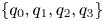 $\{ {q_0},{q_1},{q_2},{q_3}\} $:
 \begin{equation}{\varPsi ^ + } = \begin{pmatrix} { - F_x^ + + iF_y^ + }\\ {F_z^ + }\\ {F_z^ + }\\ {F_x^ + + iF_y^ + } \end{pmatrix}\equiv \begin{pmatrix} {{q_0}}\\ {{q_1}}\\ {{q_2}}\\ {{q_3}} \end{pmatrix}.\end{equation}
Equation (1.10) for homogeneous media (and with no external sources) reduces to (on setting c = 1)
 \begin{equation}\frac{\partial }{{\partial t}}\begin{pmatrix} {{q_0}}\\ {{q_1}}\\ {{q_2}}\\ {{q_3}} \end{pmatrix} = - \frac{\partial }{{\partial x}}\begin{pmatrix} {{q_2}}\\ {{q_3}}\\ {{q_0}}\\ {{q_1}} \end{pmatrix} + i\frac{\partial }{{\partial y}}\begin{pmatrix} {{q_2}}\\ {{q_3}}\\ { - {q_0}}\\ { - {q_1}} \end{pmatrix} - \frac{\partial }{{\partial z}}\begin{pmatrix} {{q_0}}\\ {{q_1}}\\ { - {q_2}}\\ { - {q_3}} \end{pmatrix}.\end{equation}
Note the overall similarity with the Dirac equation for a massless particle, (2.2).
A QLA for the Maxwell equations, (2.4), can now be readily determined, building on the Dirac-QLA of Yepez (Reference Yepez2002, Reference Yepez2005, Reference Yepez2016). Here we concentrate on determining such an algorithm of interleaved unitary collision-stream operators for one- (1-D) and two-dimensional (2-D) Maxwell equations. In particular, we note the following coupling of the qubits between the time derivative  $\partial /\partial t$ and the spatial derivatives
 $\partial /\partial x,\partial /\partial y$ in (2.4):
 \begin{equation}{q_0} \leftrightarrow {q_2},\quad {q_1} \leftrightarrow {q_3}.\end{equation}
Hence, we introduce unitary collision matrices that entangle these qubits locally at each lattice site:
 \begin{align}{C_X} = \begin{pmatrix} {\cos \theta }&0&{\sin \theta }&0\\ 0&{\cos \theta }&0&{\sin \theta }\\ { - \sin \theta }&0&{\cos \theta }&0\\ 0&{ - \sin \theta }&0&{\cos \theta } \end{pmatrix},\quad {C_Y} = \begin{pmatrix} {\cos \theta }&0&{i\sin \theta }&0\\ 0&{\cos \theta }&0&{i\sin \theta }\\ {i\sin \theta }&0&{\cos \theta }&0\\ 0&{i\sin \theta }&0&{\cos \theta } \end{pmatrix}.\end{align}
The unitary streaming operators will stream half of the qubits at each operation: because of the collision coupling  ${q_0} \leftrightarrow {q_2},\;{q_1} \leftrightarrow {q_3}$ we will first stream
 $\{ {q_0},\;{q_1}\}$ leaving
 $\{ {q_2},\;{q_3}\}$ fixed at the local lattice site. We will then stream
 $\{ {q_2},\;{q_3}\}$, leaving
 $\{ {q_0},\;{q_1}\}$ fixed. Thus, we introduce the unitary streaming operators
 $S_{ \pm X}^{01},\;S_{ \pm X}^{23}$ for propagation of the collisional entanglement along the lattice in the x-direction by
 $\pm 1$ lattice units:
 \begin{align}S_{ \pm X}^{01}\begin{pmatrix} {{q_0}(x,y,t)}\\ {{q_1}(x,y,t)}\\ {{q_2}(x,y,t)}\\ {{q_3}(x,y,t)} \end{pmatrix} = \begin{pmatrix} {{q_0}(x \pm 1,y,t)}\\ {{q_1}(x \pm 1,y,t)}\\ {{q_2}(x,y,t)}\\ {{q_3}(x,y,t)} \end{pmatrix},\quad S_{ \pm X}^{23}\begin{pmatrix} {{q_0}(x,y,t)}\\ {{q_1}(x,y,t)}\\ {{q_2}(x,y,t)}\\ {{q_3}(x,y,t)} \end{pmatrix}= \begin{pmatrix} {{q_0}(x,y,t)}\\ {{q_1}(x,y,t)}\\ {{q_2}(x \pm 1,y,t)}\\ {{q_3}(x \pm 1,y,t)} \end{pmatrix}.\end{align}
Similarly, for the unitary streaming operators in the y-direction:  $S_{ \pm Y}^{01},\;S_{ \pm Y}^{23}$.
Owing to the separability of the Cartesian orthogonal coordinates we can consider the interleaving of the collision-streaming operators for each direction separately. For the x-direction, one considers
 \begin{equation}\left. \begin{gathered} {{U_X} = S_{ - X}^{01}{C_X}S_{ + X}^{01}C_X^{\dagger} \cdot S_{ + X}^{23}{C_X}S_{ - X}^{23}C_X^{\dagger} }\\ {U_X^{\textrm{adj}} = S_{ + X}^{01}C_X^{\dagger} S_{ - X}^{01}{C_X} \cdot S_{ - X}^{23}C_X^{\dagger} S_{ + X}^{23}{C_X}} \end{gathered}\right\},\end{equation}
so that for small collision angle  $\theta \sim \varepsilon \ll 1$,
 \begin{equation}{U_X} = {I_4} - \frac{{{\varepsilon ^2}}}{2}\begin{pmatrix} 0&{{I_2}}\\ {{I_2}}&0 \end{pmatrix}\frac{\partial }{{\partial x}} + O({\varepsilon ^3}),\end{equation}
where  ${I_n}$ is the n-dimensional identity matrix. To remove
 $O({\varepsilon ^3})$ terms so as to have a second-order accurate scheme, we symmetrize the collide-stream sequence of operators in
 ${U_X}$ so that
 \begin{equation}U_X^{\textrm{adj}}{U_X} = {I_4} - {\varepsilon ^2}\begin{pmatrix} 0&{{I_2}}\\ {{I_2}}&0 \end{pmatrix}\frac{\partial }{{\partial x}} + O({\varepsilon ^4}).\end{equation}
Recognizing the differences between the Pauli spin matrices  ${\sigma _x},\;{\sigma _y}$, (1.8a–c), and the different signs of the qubit couplings in (2.4), we consider a slightly different sequence of interleaved operators:
 \begin{equation}\left. \begin{gathered} {{U_Y} = S_{ - Y}^{23}{C_Y}S_{ + Y}^{23}C_Y^{\dagger} \cdot S_{ + Y}^{01}{C_Y}S_{ - Y}^{01}C_Y^{\dagger} }\\ {U_Y^{\textrm{adj}} = S_{ + Y}^{23}C_Y^{\dagger} S_{ - Y}^{23}{C_Y} \cdot S_{ - Y}^{01}C_Y^{\dagger} S_{ + Y}^{01}{C_Y}} \end{gathered} \right\},\end{equation}
so that
 \begin{equation}U_Y^{\textrm{adj}}{U_Y} = {I_4} + i{\varepsilon ^2}\begin{pmatrix} 0&{{I_2}}\\ { - {I_2}}&0 \end{pmatrix}\frac{\partial }{{\partial y}} + O({\varepsilon ^4}).\end{equation}
The QLA time advancement of the 4-spinor components
 \begin{equation}\begin{pmatrix} {q_0}\\ {q_1}\\ {q_2}\\ {q_3} \end{pmatrix}_{t + \delta t} = U_Y^{\textrm{adj}}{U_Y}U_X^{\textrm{adj}}{U_X}\begin{pmatrix} {q_0}\\ {q_1}\\ {q_2}\\ {q_3} \end{pmatrix}_t,\end{equation}
yields the required evolution of the 4-spinor
 \begin{equation}\frac{\partial }{{\partial t}}\begin{pmatrix} {q_0}\\ {q_1}\\ {q_2}\\ {q_3} \end{pmatrix}= -\frac{\partial }{{\partial x}}\begin{pmatrix} {q_2}\\ {q_3}\\ {q_0}\\ {q_1} \end{pmatrix} + i\frac{\partial }{{\partial y}}\begin{pmatrix} {q_2}\\ {q_3}\\ - {q_0}\\ - {q_1} \end{pmatrix} + O({\varepsilon ^2}),\end{equation}
provided we have diffusion scaling (time advancement  $\delta t \sim {\varepsilon ^2}$ with lattice spacing
 $\delta x = \delta y \sim \varepsilon$) and collision angle
 $\theta = \varepsilon /4$. Equation (2.14) is just Maxwell equations for electromagnetic fields with 2-D spatial dependence in x–y.
3. QLA simulation of propagation of Gaussian wave packet for the 2-D Maxwell equations in a vacuum
First, we shall consider a Gaussian wave packet propagating in the y-direction with initial conditions,
 \begin{equation}\left. \begin{gathered} {{E_z}(x,y,t = 0) = {E_0}\exp \left[ { - \dfrac{{{{(y - {y_0})}^2}}}{{{\sigma^2}}}} \right]\cos [{k_y}(y - {y_0})]}\\ {{B_x}(x,y,t = 0) = {E_z}(x,y,t = 0)} \end{gathered} \right\},\end{equation}
and the other field components zero:  ${E_x} = 0 = {E_y} = {B_y} = {B_z}$. The 2-D QLA algorithm, (2.13), is solved on a 5000 × 5000 grid, with the small parameter
 $\varepsilon = 0.1$ and collision angle
 $\theta = \varepsilon /4$. For parameters
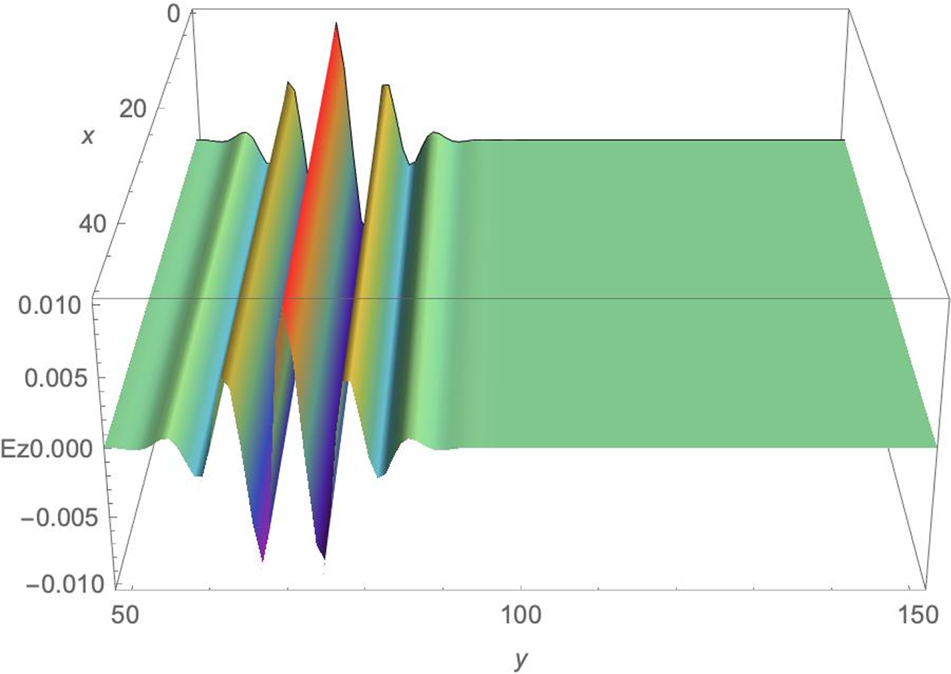
 ${E_0} = 0.01,\;{\sigma ^2} = 9000,\;{k_y} = 0.08$, the initial Gaussian wave packet for EZ is shown in figure 1, where
 ${E_z}(x,y,t) = Re [{q_1} + {q_2}]/2$.
The initial Gaussian wave packet for the electric field  ${E_z}(x,y,t = 0)$, plotted at every tenth data point in the x- and y-directions (i.e. the actual simulation grid is 500 < y
 $^{\prime}$ < 1500, 0 < x
 $^{\prime}$ < 500).

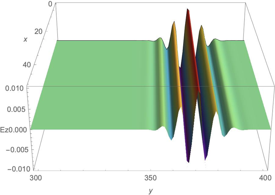
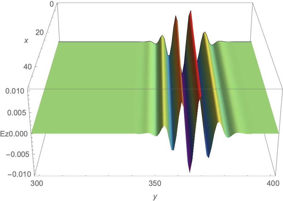
After 30 000 time steps, under periodic boundary conditions, the wave packet has propagated along the y-axis undistorted, as shown in figure 2. The 2D QLA does not spread or amplify any x-dependent noise throughout the simulation even after 130 000 time steps, as shown in figure 3.
The EZ-component of the Gaussian wave packet at t = 30 000.

The EZ-component of the Gaussian wave packet at t = 130 000.

It is interesting to note that while the evolution equations for the spinor amplitudes q 1 and q 2 in (2.14) are explicitly different, 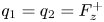 ${q_1} = {q_2} = F_z^ +$, as seen in (2.3). Indeed, QLA simulations show
 $|Re [{q_1} - {q_2}]|\lt {10^{ - 6}}$. A 500 000 iteration run was performed for 2-D QLA to test its unitarity and energy conservation. We find unitarity is well preserved with slight variations in the 10th significant figure, whereas the Poynting flux
 $\boldsymbol{S}\boldsymbol{\cdot}\boldsymbol{\hat{n}} = \int {\textrm{d}x\,\textrm{d}y\boldsymbol{E} \times \boldsymbol{B}\boldsymbol{\cdot}\boldsymbol{\hat{n}}}$ is conserved to the sixth significant figure. In our normalized units,
 ${B_x} = {E_z}$ and this is faithfully preserved in the QLA simulations.
4. QLA for 1-D Maxwell equations in inhomogeneous media
We now turn to the case of normal incidence of an electromagnetic wave onto a dielectric boundary, permitting only a spatial dependence in x, i.e. we consider an electromagnetic wave with non-zero components  ${E_y}(x,t),{B_z}(x,t)$ propagating in a medium with refractive index
 $n(x)$. Equations (1.6)–(1.8a–c) reduce to the following 8-spinor representation which is conveniently written in the two polarization blocks of 4-spinor components:
 \begin{gather}\frac{\partial }{{\partial t}}\begin{pmatrix} {q_0}\\ {q_1}\\ {q_2}\\ {q_3} \end{pmatrix} = - \frac{1}{{n(x)}}\frac{\partial }{{\partial x}}\begin{pmatrix} {q_2}\\ {q_3}\\ {q_0}\\ {q_1} \end{pmatrix} - \frac{{n^{\prime}(x)}}{{2{n^2}(x)}}\begin{pmatrix} {q_1} + {q_6}\\ {q_0} - {q_7}\\ {q_3} - {q_4}\\ {q_2} + {q_5} \end{pmatrix},\end{gather}
 \begin{gather}\frac{\partial }{{\partial t}}\begin{pmatrix} {q_4}\\ {q_5}\\ {q_6}\\ {q_7} \end{pmatrix} = - \frac{1}{{n(x)}}\frac{\partial }{{\partial x}}\begin{pmatrix} {q_6}\\ {q_7}\\ {q_4}\\ {q_5} \end{pmatrix} - \frac{{n^{\prime}(x)}}{{2{n^2}(x)}}\begin{pmatrix} {q_5} + {q_2}\\ {q_4} - {q_3}\\ {q_7} - {q_0}\\ {q_6} + {q_1} \end{pmatrix},\end{gather}
where  $n^{\prime}(x) = \textrm{d}n/\textrm{d}x$, and
 \begin{equation}\begin{pmatrix} {{q_0}}\\ {{q_1}}\\ {{q_2}}\\ {{q_3}}\\ {{q_4}}\\ {{q_5}}\\ {{q_6}}\\ {{q_7}} \end{pmatrix} = \begin{pmatrix} { - F_x^ + + iF_y^ + }\\ {F_z^ + }\\ {F_z^ + }\\ {F_x^ + + iF_y^ + }\\ { - F_x^ - - iF_y^ - }\\ {F_z^ - }\\ {F_z^ - }\\ {F_x^ - - iF_y^ - } \end{pmatrix},\quad \textrm{with}\;{\boldsymbol{F}^ \pm } = \frac{1}{{\sqrt 2 }}\left[ {\sqrt \varepsilon \boldsymbol{E} \pm i\frac{\boldsymbol{B}}{{\sqrt \mu }}} \right].\end{equation}
The two RS vectors for the polarizations,  ${\boldsymbol{F}^+}\;\textrm{and}\;{\boldsymbol{F}^ - }$, are coupled by the spatial gradient in the refractive index
 $n(x) = \sqrt {{\mu _0}\varepsilon (x)}$. For simplicity, we consider normal wave incidence from a region of constant dielectric n 0 onto a region of constant dielectric n 1. These two dielectrics are connected by a thin boundary region [see (5.1) for its explicit profile].
The QLA that will recover the  $\partial /\partial t$ and
 $\partial /\partial x$ terms in the 1-D Maxwell equations, (4.2), has the following unitary block-diagonal collision operator,
 \begin{equation}{C_{XX}}(\theta ) = \begin{pmatrix} {{C_X}(\theta )}&0\\ 0&{{C_X}(\theta )} \end{pmatrix},\end{equation}
where  ${C_X}(\theta )$ is the 4 × 4 unitary matrix in (2.6a,b). The block-diagonal structure arises from the fact that one requires an
 $n^{\prime}(x) \ne 0$ to couple the two electromagnetic field polarizations. The collision angle is
 \begin{equation}\theta = \frac{\varepsilon }{{4n(x)}}.\end{equation}
To determine the streaming operators one notes that the qubits occurring in the  $\partial /\partial t$ and
 $\partial /\partial x$ terms of (4.2) have the coupling
 ${q_0} \leftrightarrow {q_2},\;{q_1} \leftrightarrow {q_3},\;{q_4} \leftrightarrow {q_6},\;{q_5} \leftrightarrow {q_7}$. Consequently, we choose two unitary streaming operators: one that acts on the 4-qubits
 $[{q_0},{q_1},{q_4},{q_5}]$ while the other acts on the remaining 4-qubits
 $[{q_2},{q_3},{q_6},{q_7}]$. These streaming operators will be interleaved with the collision matrix
 ${C_{XX}}(\theta )$ and its adjoint
 $C_{XX}^{\dagger}$.
The first term involving the inhomogeneous dielectric factor  $n^{\prime}(x)$ in (4.2) is recovered by the potential operator
 ${V_{11}}$which couples
 ${q_0} \leftrightarrow {q_1},\;{q_2} \leftrightarrow {q_3},\;{q_4} \leftrightarrow {q_5},\;{q_6} \leftrightarrow {q_7}$,
 \begin{align}{V_{11}}(\alpha ) =\! \begin{pmatrix} {\cos \alpha }&{ - \sin \alpha }&0&0&0&0&0&0\\ { - \sin \alpha }&{\cos \alpha }&0&0&0&0&0&0\\ 0&0&{\cos \alpha }&{ - \sin \alpha }&0&0&0&0\\ 0&0&{ - \sin \alpha }&{\cos \alpha }&0&0&0&0\\ 0&0&0&0&{\cos \alpha }&{ - \sin \alpha }&0&0\\ 0&0&0&0&{ - \sin \alpha }&{\cos \alpha }&0&0\\ 0&0&0&0&0&0&{\cos \alpha }&{ - \sin \alpha }\\ 0&0&0&0&0&0&{ - \sin \alpha }&{\cos \alpha } \end{pmatrix}\!,\end{align}
whereas the second term involving  $n^{\prime}(x)$ couples the qubits
 ${q_0} \leftrightarrow {q_6},\;{q_1} \leftrightarrow {q_7},\;{q_2} \leftrightarrow {q_4}, \;{q_3} \leftrightarrow {q_5}$ and, thus, the two electromagnetic field polarizations. It is recovered by the operator
 ${V_{22}}$,
 \begin{align}{V_{22}}(\alpha ) = \begin{pmatrix} {\cos \alpha }&0&0&0&0&0&{ - \sin \alpha }&0\\ 0&{\cos \alpha }&0&0&0&0&0&{\sin \alpha }\\ 0&0&{\cos \alpha }&0&{\sin \alpha }&0&0&0\\ 0&0&0&{\cos \alpha }&0&{ - \sin \alpha }&0&0\\ 0&0&{ - \sin \alpha }&0&{\cos \alpha }&0&0&0\\ 0&0&0&{\sin \alpha }&0&{\cos \alpha }&0&0\\ {\sin \alpha }&0&0&0&0&0&{\cos \alpha }&0\\ 0&{ - \sin \alpha }&0&0&0&0&0&{\cos \alpha } \end{pmatrix}.\end{align}
To recover the QLA for (4.2) one now needs to choose the rotation angle
 \begin{equation}\alpha = {\varepsilon ^2}\frac{{n^{\prime}(x)}}{{2{n^2}(x)}}.\end{equation}
Note that the operator  ${V_{22}}$ is unitary, whereas the operator
 ${V_{11}}$ is Hermitian but not unitary. A Hermitian matrix can be decomposed into a sum of two unitary matrices. For example, on normalizing
 ${V_{11}}$ so that
 $||{V_{11}}||\le 1$, one can rewrite
 \begin{equation}{V_{11}} = {\textstyle{1 \over 2}}(U_{11}^{(1)} + U_{11}^{(2)}),\end{equation}
where  $U_{11}^{(1)}$ and
 $U_{11}^{(2)}$ are unitary with
 \begin{equation}U_{11}^{(1)} = {V_{11}} + i\sqrt {I - V_{11}^2} ,\quad U_{11}^{(2)} = {V_{11}} - i\sqrt {I - V_{11}^2} .\end{equation}
Childs & Wiebe (Reference Childs and Wiebe2012) have shown that linear combinations of unitary operators can be encoded on quantum computers and, in some cases, these algorithms can outperform the usual product of unitary operators algorithms, particularly for sparse matrices.
Denoting the unitary streaming operator  $S_{ + X}^{01,45}$ that shifts qubits
 $[{q_0},{q_1};{q_4},{q_5}]$ one lattice unit in the +x-direction while keeping the other four qubits fixed, and
 $S_{ - X}^{23,67}$ the streaming operator on the qubits
 $[{q_2},{q_3};{q_6},{q_7}]$ one lattice unit in the −x direction, we consider the following unitary interleaved sequence of unitary collide-stream operators
 \begin{equation}\begin{array}{l} {{U_{XX}} = S_{ - X}^{01,45}{C_X}(\theta ) \cdot S_{ + X}^{01,45}C_X^{\dagger} (\theta ) \cdot S_{ + X}^{23,67}{C_X}(\theta ) \cdot S_{ - X}^{23,67}C_X^{\dagger} (\theta )}\\ {U_{XX}^{\textrm{adj}} = S_{ + X}^{01,45}C_X^{\dagger} (\theta ) \cdot S_{ - X}^{01,45}{C_X}(\theta ) \cdot S_{ - X}^{23,67}C_X^{\dagger} (\theta ) \cdot S_{ + X}^{23,67}{C_X}(\theta )} \end{array},\quad \textrm{with}\;\theta = \frac{\varepsilon }{{4n(x)}}.\end{equation}
On incorporating the potential operators  ${V_{11}}(\alpha )$ and
 ${V_{22}}(\alpha )$, (4.6) and (4.7), the final 1-D QLA for Maxwell equations with propagation in the x-direction becomes
 \begin{equation}\textrm{QLA}:{\boldsymbol{\mathsf{q}}}(t + \delta t) = {V_{22}}(\alpha ) \cdot {V_{11}}(\alpha ) \cdot U_{XX}^{\textrm{adj}}{U_{XX}} {\boldsymbol{\mathsf{q}}}(t),\end{equation}
where  ${\boldsymbol{\mathsf{q}}}$ is the 8-spinor defined in (4.3).
5. QLA simulations for 1-D inhomogeneous dielectric media
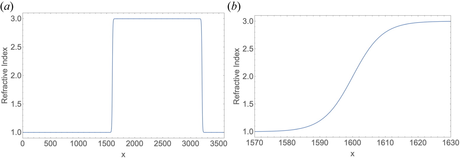
We now present some 1-D QLA simulations of electromagnetic fields propagating in the x-direction from a region of low refractive index n 0 into a region of higher refractive index n 1. Such a refractive index profile is modelled by the hyperbolic tangent function,
 \begin{equation}n(x) = \frac{{{n_0} + {n_1}}}{2} - \frac{{{n_0} - {n_1}}}{2}\tanh [\beta (x - {L_m})],\end{equation}
where  $\beta $ controls the thickness of the boundary region between the two media. Some care needs to be taken with the perturbation parameter
 $\varepsilon $, as the collide-stream unitary operators have
 $\theta = O(\varepsilon )$ whereas the operators controlling the media refractive interface have
 $\alpha = O({\varepsilon ^2})$ – one order of
 $\varepsilon$ appearing implicitly from the scaling of
 $n^{\prime}(x)$. For the simulations reported here, the boundary region between the two media is centred at
 ${L_m} = 1600$ (lattice units) with the end of the grid at
 ${L_{\textrm{end}}} = 2{L_m}$. Periodic boundary conditions are enforced by adding a small buffer region after L end so that the refractive index is periodic, as shown in figure 4(a)
(a) Refractive index profile and (b) blow-up of the boundary region between media.

5.1. Gaussian electromagnetic pulse
First, consider a simple Gaussian pulse propagating from the region of refractive index  ${n_0} = 1$ towards the region with
 ${n_1} = 3$, with
 $\varepsilon = 0.3$. The initial electric and magnetic field profiles are solutions of the Maxwell equations with
 ${B_z}(x,0) = n(x){E_y}(x,0)$ and
 \begin{equation}{E_y}(x,0) = {E_0}\exp \left[ { - \frac{{{{(x - {x_0})}^2}}}{{{\sigma^2}}}} \right].\end{equation}
We choose  ${E_0} = 0.01$, with the centre of the pulse at
 ${x_0} = 700$ and pulse width of 600 lattice units (controlled by
 ${\sigma ^2} = 50\;000$). The centre of the dielectric boundary layer is at
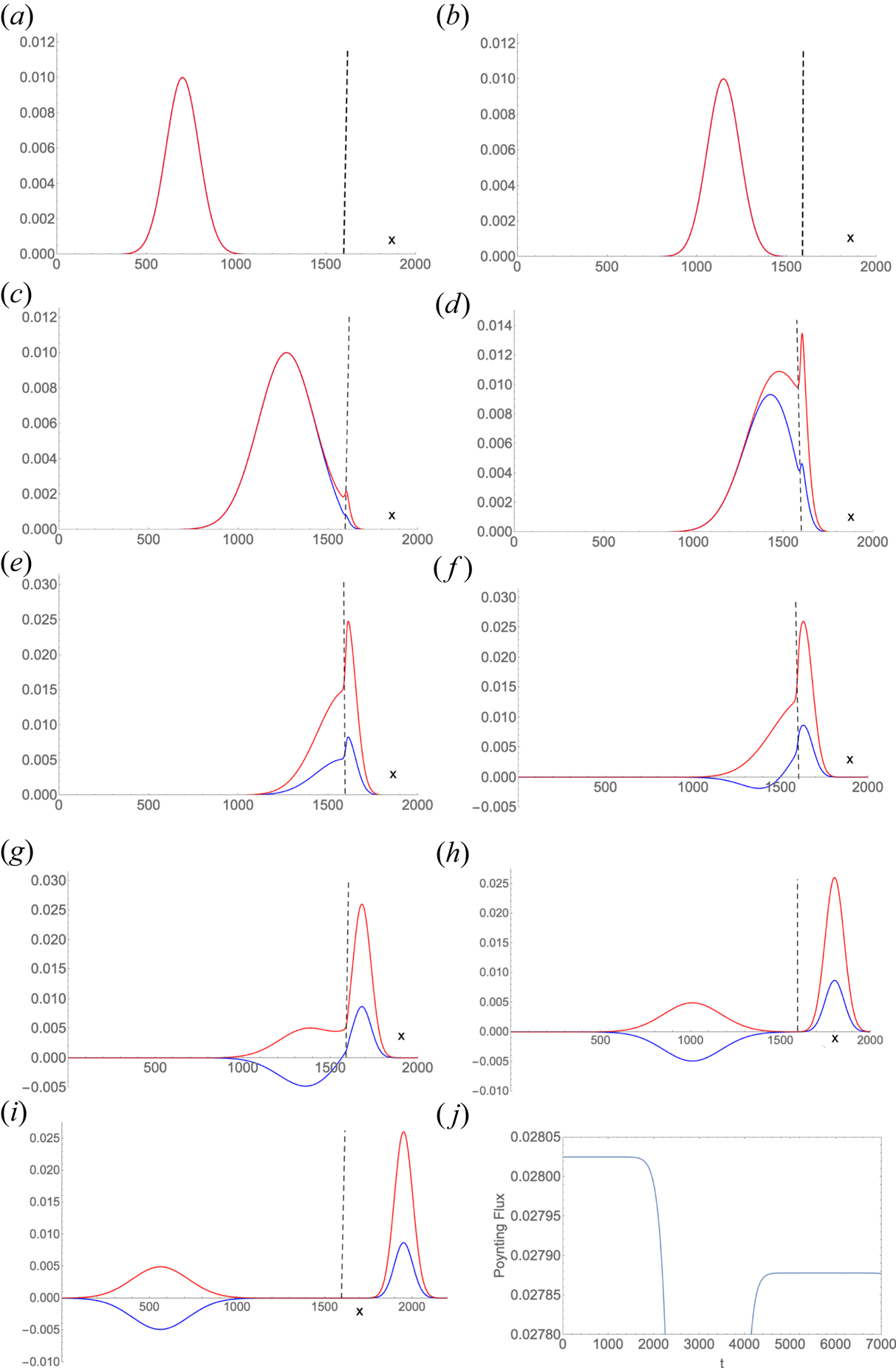
 ${L_m} = 1600$ and is shown in figure 5 as a vertical dashed line. The width of the dielectric boundary layer is ~40 lattice units.
The propagation of the  ${E_y}$-field of an electromagnetic pulse from vacuum into a dielectric region with n 1 = 3. The interface is at x = 1600 (dashed vertical line). (a) Initially the field components are identical:
 ${E_y}$ (blue) =
 ${B_z}$ (red). (b) The pulse propagates undistorted in the vacuum. (c) Overlap with the dielectric boundary layer occurs by t = 1900. (d) By t = 2500 the back of the pulse is still incident onto the dielectric interface while the front part of the pulse is being reflected back into the vacuum region. (e) For times t ≥ 3000 the incident pulse has evolved into a reflected (x < 1600) and a transmitted pulse (x > 1600). (f) At t = 3300, the reflected
 ${E_y}$ begins its phase reversal, and which is completed by t = 3800. (g) Full phase reversal in the reflected
 ${E_y}$ has almost been achieved by t = 3800. (h) The asymptotic state at t = 5000. (i) At t = 6500 one sees the transmitted pulse's width is 1/3 of the initial (and reflected) pulse, whereas its velocity is 1/3 of the velocity of the initial (and reflected) pulse. (j) The instantaneous Poynting flux,
 $\boldsymbol{S}(t)\boldsymbol{\cdot}\boldsymbol{\hat{n}} = \int {\textrm{d}x} \boldsymbol{E} \times \boldsymbol{B}\boldsymbol{\cdot}\boldsymbol{\hat{n}}$, showing very good energy conservation of the asymptotic state.

The pulse propagates undistorted in vacuum as it moves towards the dielectric boundary, figure 5(a,b). This indicates that the parameters for QLA have been so chosen that it perturbatively recovers the Maxwell equations. As the leading edge of the pulse encounters the dielectric layer, figure 5(c), part of it is reflected (transiently producing unequal reflected  ${E_y}$ and
 ${B_z}$ fields) and part of it is transmitted. At t = 2500, figure 5(d), the first half of the pulse undergoes reflection and transmission while the trailing half of the pulse is still propagating towards the dielectric boundary (because for x < 1250 one has
 ${E_y} = {B_z}$). At t = 3000, figure 5(e), we have a transient reflected and transmitted pulses, but as yet no phase reversal in the reflected
 ${E_y}$. The start of the phase reversal is clearly seen at t = 3300, figure 5(f). By the time t = 3800, figure 5(g) there is a complete phase reversal in
 ${E_y}$. However, the asymptotic
 ${\rm \pi}$-phase change occurs by t = 5000, figure 5(h). Figure 5(i) shows that the reflected pulse has a velocity three times that of the transmitted pulse, with the peak of the transmitted
 ${B_z}$ being three times the peak of the transmitted
 ${E_y}$. Moreover, both the reflected and transmitted waves travel undistorted in their respective constant dielectric media, indicating that the QLA is not introducing spurious noise into the simulation. The instantaneous Poynting flux, figure 5(j) shows that, in the asymptotic state, energy is conserved to within 0.5 %. In the asymptotic state we have simply reflected and transmitted pulses which have well-defined constant normal. In the time interval 2000 < t < 4000, the pulse overlaps the dielectric boundary layer, with the leading part of the pulse starting to experience reflection (with the normal now in the negative x-direction) while the trailing part of the pulse is still incident (with its normal in the positive x-direction). This leads to a time-varying normal direction, which is non-trivial to define, leading to a difficulty in determining the instantaneous Poynting flux. However, it is the initial and asymptotic Poynting flux that is most relevant.
It is worthwhile to compare the QLA simulations of a Gaussian pulse propagating towards a strongly varying but continuous dielectric region with the standard electromagnetic plane wave solution for normal incidence onto a dielectric discontinuity (Jackson Reference Jackson1998). Assuming that there are only an incident, reflected and transmitted plane waves, kinematics requires that the ratio of the wavelength of the transmitted plane wave to that of the incident wave be  ${\lambda _{\textrm{trans}}}/{\lambda _{\textrm{inc}}} = {n_0}/{n_1} = 1/3$. The jump conditions on the amplitudes of the plane waves follow from Maxwell equations and the boundary conditions at the discontinuous dielectric interface,
 \begin{equation}\frac{{{E_{\textrm{refl}}}}}{{{E_{\textrm{inc}}}}} = \frac{{{n_0} - {n_1}}}{{{n_0} + {n_1}}} = - \frac{1}{2},\quad \frac{{{E_{\textrm{trans}}}}}{{{E_{\textrm{inc}}}}} = \frac{{2{n_0}}}{{{n_0} + {n_1}}} = + \frac{1}{2}\quad \textrm{for}\;{n_0} = 1,\;{n_1} = 3,\end{equation}
with
 \begin{equation}\frac{{{B_{\textrm{refl}}}}}{{{E_{\textrm{refl}}}}} = - 1,\quad \frac{{{B_{\textrm{trans}}}}}{{{E_{\textrm{trans}}}}} = 3.\end{equation}
From the 1-D QLA simulations of a Gaussian pulse, we find that (at t = 6500, figure 5i) the peaks of the fields occur at the same lattice point (at x = 561 for the reflected wave and at x = 1950 for the transmitted wave) with amplitude ratios,
 \begin{equation}\frac{{{B_{\textrm{refl}}}}}{{{E_{\textrm{refl}}}}} = - \frac{{4.90362}}{{4.90361}},\quad \frac{{{B_{\textrm{trans}}}}}{{{E_{\textrm{trans}}}}} = \frac{{2.60122}}{{0.86708}} = 2.999994,\end{equation}
while
 \begin{equation}\frac{{{E_{\textrm{refl}}}}}{{{E_{\textrm{inc}}}}} = - \frac{{4.90361}}{{10}} = - 0.49,\quad \frac{{{E_{\textrm{trans}}}}}{{{E_{\textrm{inc}}}}} = \frac{{8.67075}}{{10}} = 0.87.\end{equation}
These QLA results are in excellent agreement with the standard plane wave theory except for the ratio of the transmitted to the incident amplitudes  ${E_{\textrm{trans}}}/{E_{\textrm{inc}}}$. The QLA yields 0.87 for the ratio, whereas the plane wave theory yields 0.5. We attribute this to the fundamental difference between a Gaussian pulse, which is composed of an infinite set of plane waves, and a single plane wave.
5.2. Propagation of a Gaussian wave packet
We now consider the propagation of a Gaussian wave packet, whose envelope is the Gaussian pulse considered in § 5.1. The initial electric field is taken to be
 \begin{equation}{E_y}(x,0) = {E_0}\exp \left[ { - \frac{{{{(x - {x_0})}^2}}}{{{\sigma^2}}}} \right] \cdot \cos [{k_x}(x - {x_0})]r,\end{equation}
with  ${k_x} = 0.06$.
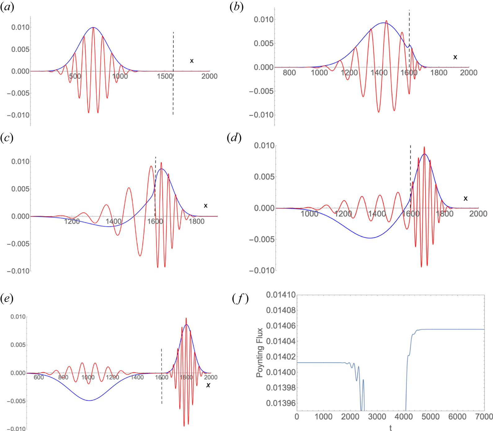
The wavelength compression of the transmitted field (x > 1600) by  $1/{n_1} = 1/3$ is evident in figure 6(b–e). The instantaneous lattice-averaged Poynting flux, figure 6(f), shows very good energy conservation to within 0.4 %. Within the transition layer, the intermixing of the incident, reflected, and transmitted waves does not permit the proper determination of the unit normal direction
 $\boldsymbol{\hat{n}}(t)$. Again, it is important to note that QLA does not introduce spurious noise in the time evolution of the asymptotic state.
The evolution of  ${E_y}$ of a Gaussian wave packet (in red) and of its initial envelope (in blue) in vacuum as the wave packet propagates towards a region of
 ${n_1} = 3$. The transition layer and the evolution of the envelope solution is as discussed earlier (figures 4 and 5): (a) t = 0; (b) t = 2500, there is a wavelength contraction of the transmitted field owing to the higher refractive index of the medium; (c) t = 3300, (d) t = 3800, (e) t = 5000, asymptotic state; and (f) the time evolution of the lattice averaged Poynting flux. The asymptotic states show conservation of energy to within 0.4 %.

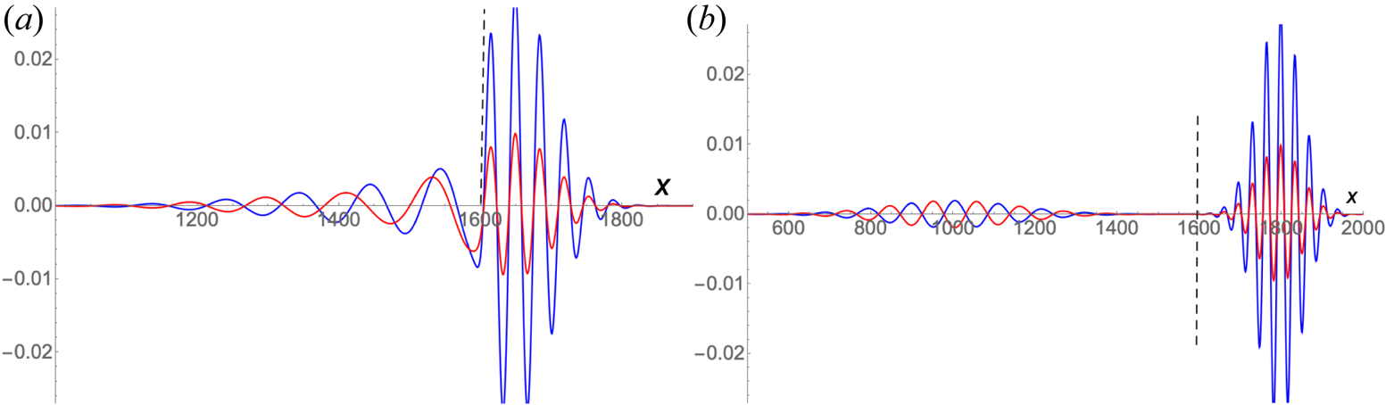
Finally in figure 7(a) we show the corresponding Gaussian wave packet fields  ${E_y},{B_z}$ at a time of significant overlap of the packet over the two dielectric regions, while in figure 7(b) we show the asymptotic state of
 ${E_y}(\textrm{red}),\;{B_z}(\textrm{blue})$. It is apparent that at t = 5000 we see the full
 ${\rm \pi}$-reversal in the phase of
 ${E_y}$.
The (a)  ${E_y}$ (red) and
 ${B_z}$ (blue) profiles during the overlap of the Gaussian wave packet over the dielectric boundary at t = 3500. The transmitted fields are in phase whereas the reflected fields have transient phases. (b) For the asymptotic state, t = 5000, the reflected
 ${E_y}$ field is
 ${\rm \pi}$ out of phase with
 ${B_z}$ and the incident fields.

Again there is excellent agreement with plane wave theory, (5.3a,b) and (5.4a,b), for
 \begin{equation}\textrm{QLA}:\frac{{{B_{\textrm{refl}}}}}{{{E_{\textrm{refl}}}}} = - 1.00001,\quad \frac{{{B_{\textrm{trans}}}}}{{{E_{\textrm{trans}}}}} = 2.999999,\end{equation}
while there is deviation from the plane wave results, (5.3a,b), for
 \begin{equation}\textrm{QLA}:\frac{{{E_{\textrm{refl}}}}}{{{E_{\textrm{inc}}}}} = - 0.19,\quad \frac{{{E_{\textrm{trans}}}}}{{{E_{\textrm{inc}}}}} = 0.76.\end{equation}
Again, this illustrate the difference between a plane wave and a Gaussian wave packet that is composed of an infinite set of planes waves with varying amplitudes.
6. Summary and conclusions
Utilizing the similarity of the spinor representation of the Dirac equation to the Maxwell equations, we have extended our studies in unitary QLA (Vahala etal. Reference Vahala, Vahala and Yepez2003a,Reference Vahala, Vahala and Yepezb, Reference Vahala, Vahala and Yepez2004, Reference Vahala, Vahala and Yepez2005, Reference Vahala, Yepez, Vahala, Soe, Zhang and Ziegeler2011, Reference Vahala, Yepez, Vahala and Soe2012a,Reference Vahala, Zhang, Yepez, Vahala and Soeb, Reference Vahala, Soe, Vahala and Yepez2019a,Reference Vahala, Vahala, Soe, Ram and Yepezb, Reference Vahala, Soe and Vahala2020a,Reference Vahala, Vahala and Soeb,Reference Vahala, Vahala, Soe and Ramc). In particular, using the Pauli spin-½ matrices, we have expressed Khan's RS representation of the Maxwell equations in a unitary spinor lattice representation. The QLA is readily determined for the 1-D and 2-D spatial dependence of the electromagnetic fields. For homogeneous media, the QLA requires only four spinor components per spatial lattice node, whereas for inhomogeneous media the two polarizations of the electromagnetic fields are coupled requiring the use of the two RS vectors and an 8-spinor representation. The QLA can be shown to be second-order accurate under diffusion ordering. To attain this ordering, we must introduce a small parameter  $\varepsilon$ into the unitary collision operators. In our earlier works of QLA for the nonlinear Schrodinger equation and Bose–Einstein condensation for spinor fields, the introduction of the required small parameter can be accomplished by an appropriate scaling of the spinor order parameter wave functions that appear in the nonlinear Bose–Einstein interaction potential (Vahala et al. Reference Vahala, Vahala and Yepez2003a,Reference Vahala, Vahala and Yepezb, Reference Vahala, Vahala and Yepez2005, Reference Vahala, Yepez, Vahala and Soe2012a,Reference Vahala, Zhang, Yepez, Vahala and Soeb, Reference Vahala, Soe, Vahala and Yepez2019a, Reference Vahala, Soe and Vahala2020a,Reference Vahala, Vahala and Soeb). For the Maxwell representation, this is not possible. By appropriately scaling the fields relative to the lattice spatial unit the QLA will still hold for sufficiently small
 $\varepsilon$.
To benchmark the QLA we have considered two problems: (1) electromagnetic propagation in a 2-D homogeneous medium, and (2) electromagnetic propagation in 1-D inhomogeneous media. In a 2-D homogeneous medium, we have tested propagation in the x-direction and y-direction separately. This was done since the Pauli spin-½ matrices  ${\sigma _x}$ are real whereas
 ${\sigma _y}$ are purely imaginary, resulting in a different collide-stream interleaved sequence in these directions to recover the 2-D QLA Maxwell equations. As the results were essentially the same, we have only presented the results for y-propagation. In 1-D inhomogeneous media, we have studied the problem of a 1-D normally incident electromagnetic wave onto a sharp (but continuous) transition region between two different dielectric media. For a Gaussian pulse, this problem would be very difficult to solve analytically. Of course, if the dielectric boundary region became a strict discontinuity, the standard electromagnetic texts solve this boundary value problem for a plane wave, yielding the appropriate phase shifts in the reflected wave and the corresponding amplitude ratios. QLA conserves energy to within 0.5 % in the asymptotic final states. The deviation in one or two field amplitude ratios of QLA from a simple single plane wave electromagnetic solution was at first somewhat unexpected, especially because the other ratios agreed with the simple plane wave solution to six significant figures. We argue that this can occur because the representation of the incident pulse by a finite set of plane waves will require a complicated set of phases to be included. The resultant sum, because of these different phases, will be different from a simple finite sum of terms without phases. Moreover, there is the question of truncation of the infinite plane wave solution and the carry-over of results from finite to infinite sums is not guaranteed.
It is interesting to compare our 1-D QLA, which utilizes simple unitary collision and streaming operators based on the Pauli spin-½ matrices, with the Jestadt et al. algorithm (Jestadt, Appel & Rubio Reference Jestadt, Appel and Rubio2014; Jestadt et al. Reference Jestadt, Ruggenthaler, Oliveira, Rubio and Appel2018) based on the bosonic spin-1 matrices. Consequently, they only consider the 3-spinor components
 \begin{equation}{\varPhi ^ \pm } = \begin{pmatrix} { - F_x^ \pm + iF_y^ \pm }\\ {F_z^ \pm }\\ {F_x^ \pm + iF_y^ \pm } \end{pmatrix}.\end{equation}
This representation recovers the time-dependent parts of Maxwell's equations, but not the divergence equations  $\boldsymbol{\nabla}\boldsymbol{\cdot }\boldsymbol{D} = \rho ,\;\boldsymbol{\nabla}\boldsymbol{\cdot }\boldsymbol{B} = 0$. These two equations will have to be imposed as constraints. For 1-D propagation these constraints are easily satisfied, but their representation in three dimensions is non-trivial. For closure, Jestadt et al. (Reference Jestadt, Appel and Rubio2014) invoke the Baker–Campbell–Hausdorff expansion to approximate the exponential operator in the commutator of their kinetic-potential operators and their inhomogeneous medium operator. This commutator depends on the second derivative on the refractive index
 $n^{\prime\prime}(y)$ with respect to y. In our QLA, it is the interleaving of the non-commuting unitary collide-stream operators that yields the Maxwell equations: if we had ignored the non-commutative property of the collision and streaming operators, then our sequence would have resulted in the identity operator itself. Extension of QLA for Maxwell equations to three dimensions is expected to follow the standard procedures we have utilized in earlier QLA for 1-D and 3-D simulations of the nonlinear Schrodinger equation (Vahala et al. Reference Vahala, Vahala and Yepez2003a,Reference Vahala, Vahala and Yepezb, Reference Vahala, Yepez, Vahala, Soe, Zhang and Ziegeler2011, Reference Vahala, Yepez, Vahala and Soe2012a,Reference Vahala, Zhang, Yepez, Vahala and Soeb, Reference Vahala, Soe, Vahala and Yepez2019a,Reference Vahala, Vahala, Soe, Ram and Yepezb, Reference Vahala, Soe and Vahala2020a,Reference Vahala, Vahala and Soeb). Other spinor representations of Maxwell equations were also attempted by Moses (Reference Moses1959), Coffey (Reference Coffey2008) and Kulyabov et al. (Reference Kulyabov, Kolokova and Sevatianov2017).
The vista for further applications is boundless as the field of electromagnetic wave propagation in different dielectric media, such as a 3D magnetized plasma, lies before us.
Acknowledgements
The 2-D simulations were performed on the DoD HPC supercomputer whereas the 1-D simulations were performed on a vintage MAC Pro and MacBook Pro. G.V., in particular, thanks J. Yepez for many fruitful discussion on QLA. L.V. was partially supported by an AFRL STTR Phase I with Semicyber LLC contract number FA864919PA049. G.V., L.V. and M.S. were partially supported by an AFRL STTR Phase 2 with Semicyber LLC contract number FA864920P0419. A.K.R. was supported by DoE Grant Number DE-FG02-91ER-54109 and DE-SC0018090. We would also like to acknowledge helpful comments from the referees that have helped improve this paper.
Editor William Dorland thanks the referees for their advice in evaluating this article.
Declaration of interests
The authors report no conflict of interest.