





1. Introduction
A wide range of flow phenomena involve a moving interface, where one fluid displaces another in quasi-two-dimensional geometries. Such interfaces can become unstable to small perturbations, giving rise to complex patterns. In shear-dominated flows, such as those occurring in Hele-Shaw cells or porous media, viscous fingering instability produces characteristic finger-like structures (Saffman & Taylor Reference Saffman and Taylor1958; Paterson Reference Paterson1981). Such instability is generally driven by the viscosity contrast between a displacing and an ambient fluid. Particularly, a configuration with a more viscous displacing fluid is known to be stable.
By contrast, under similar configurations a more viscous displacing fluid can become unstable in extensionally dominated flows, when the displacing fluid is sufficiently strain-rate softening (e.g. shear thinning), forming tearing patterns (Sayag Reference Sayag2019; Sayag & Worster Reference Sayag and Worster2019a , Reference Sayag and Worsterb ; Ball & Balmforth Reference Ball and Balmforth2021). Specifically, laboratory experiments of polymer solutions spreading into an ambient salt solution under weak interfacial traction, have shown that an initially axisymmetric front becomes unstable, developing rift-like patterns (figure 1) (Sayag et al. Reference Sayag, Pegler and Worster2012; Sayag & Worster Reference Sayag and Worster2019a ; Ball & Balmforth Reference Ball and Balmforth2021). These tearing instabilities appear in both engineering and geophysical contexts. For example, axisymmetric extrusion of concentrated pastes can produce radial tearing patterns at the unconfined edge (e.g. Mascia et al. Reference Mascia, Patel, Rough, Martin and Wilson2006). The spreading of unconfined ice shelves into the open ocean can result in the formation of radial rifts that are several orders of magnitude larger (Hughes Reference Hughes1983; Fricker et al. Reference Fricker, Young, Coleman, Bassis and Minster2005; Wearing et al. Reference Wearing, Kingslake and Worster2020), which may have significant implications for ice ablation and sea-level rise through calving and melting processes (MacAyeal et al. Reference MacAyeal, Scambos, Hulbe and Fahnestock2003; Banwell et al. Reference Banwell, MacAyeal and Sergienko2013; Rignot et al. Reference Rignot, Jacobs, Mouginot and Scheuchl2013; Walker et al. Reference Walker, Bassis, Fricker and Czerwinski2013; Borstad et al. Reference Borstad, McGrath and Pope2017).
The emergence of tearing patterns were explored theoretically as an instability of a spreading axisymmetric base flow of non-Newtonian fluids (Sayag Reference Sayag2019; Sayag & Worster Reference Sayag and Worster2019b ; Ball & Balmforth Reference Ball and Balmforth2021). Specifically, an annular layer of power-law fluid of uniform thickness and constant width, with an outer radius spreading radially with no friction is found to be linearly unstable to azimuthal perturbation (Sayag & Worster Reference Sayag and Worster2019b ). For an harmonic perturbation with an azimuthal wavenumber, the instability emerges for a particular base-state radius when the fluid exponent exceeds a critical threshold corresponding to a strain-rate softening fluid. The most-unstable wavenumber was found to be inversely proportional to the width of the base-state annulus, and weakly dependent on fluid exponents larger than the critical value. The linear instability mechanism involves the base-flow hoop stress enhancing geometric perturbations at the front regardless of the nature of the fluid. However, the instability is suppressed by normal-stress divergence, which gradually weakens as the fluid becomes more strain-rate softening, allowing the instability to emerge (Sayag & Worster Reference Sayag and Worster2019b ).
Showing that such an instability, based on linear analysis, includes the underlying physics leading to the rift patterns that were observed experimentally (Sayag & Worster Reference Sayag and Worster2019a ), requires solving the full nonlinear model numerically. Moreover, such a numerical simulation should address the impact of spatiotemporally evolving fluid thickness and front, and the effect of finite-amplitude perturbations. Numerical studies of spreading layers of extensional flows are common in the analysis of ice shelves and ice streams found in Greenland and Antarctica. Most of the numerical studies focus on the bulk flow, such as ice streams flowing into ice shelves (MacAyeal Reference MacAyeal1989), the evolution of ice shelves over millennia (Wolff et al. Reference Wolff2025), the recovery of ice shelves following a breakup (Akesson et al. Reference Akesson, Morlighem, Nilsson, Stranne and Jakobsson2022), and buttressing of glaciers by ice shelves (Greene et al. Reference Greene, Gardner, Schlegel and Fraser2022; Gudmundsson et al. Reference Gudmundsson, Barnes, Goldberg and Morlighem2023). Such studies were not designed a priori to accurately resolve front evolution, hindering the exploration of rift formation and evolution. More recent numerical techniques incorporate phase-field techniques and fracture mechanics to model fracture phenomena in ice sheets (e.g. Kachuck et al. Reference Kachuck, Whitcomb, Bassis, Martin and Price2022; Clayton et al. Reference Clayton, Duddu, Hageman and Martínez-Pañeda2025), including rift genesis near ice rises (Sondershaus et al. Reference Sondershaus, Humbert and Müller2026). Such simulations typically involve complex constitutive laws and multiple physical processes, as well as complex geometries motivated by the natural settings. Consequently, validating such simulations with analytical tools or laboratory experiments becomes much more challenging, and the leading order mechanism underlying fracture formation becomes much less transparent.
In Part 1 of this study (Stern et al. Reference Stern, Gudmundsson and Sayag2025), we addressed these issues in a numerical simulation aimed to explore the formation of rifts. Specifically, we explored radially spreading extensional flows of Newtonian fluids, resolving the full nonlinear evolution with spatiotemporally varying thickness, while carefully tracing the fluid front. We used an annular geometry, corresponding to the experimental and theoretical extensional regime in earlier studies (Pegler & Worster Reference Pegler and Worster2012; Sayag et al. Reference Sayag, Pegler and Worster2012; Sayag & Worster Reference Sayag and Worster2019a , Reference Sayag and Worsterb ), which allows thorough validation of the simulation with known analytical solutions. That analysis demonstrated that Newtonian flows remain globally stable under harmonic perturbations independently of the base-state radius, perturbation amplitudes or wavenumbers, and that the secondary flow is organised in regular eddies consistently with linear stability predictions. Under large-amplitude perturbations, nonlinear contributions led to the formation of cusps along perturbation crests, and the secondary flow turned more erratic, though still with regular eddies distributed along the front (Stern et al. Reference Stern, Gudmundsson and Sayag2025).
Snapshots from a laboratory experiment (Sayag & Worster Reference Sayag and Worster2019a ), showing the evolution of tongues and rifts in a radially spreading extensional flow of xanthan-gum solution (concentration 1 % in weight). Numbers at the bottom right mark the time since the start of the experiment in seconds.

A strain-rate softening fluid is predicted to be linearly unstable, and experimental evidence show that tearing patterns arise (Sayag & Worster Reference Sayag and Worster2019a , Reference Sayag and Worsterb ). Here, we explore such flows numerically by extending Part 1 to analyse the nonlinear stability of power-law fluids. We solve the same flow model under the shallow-shelf approximation (SSA), but extended to account for strain-rate dependent viscosity. We then analyse the evolution of the flow due to finite-amplitude perturbations to an initially axisymmetric state, as well as the effect of the fluid exponent and the boundary conditions on the resulted patterns. We also explore the spatiotemporal distribution of the critical stress and force components, and derive new insights on the instability mechanism.
2. Theoretical model
2.1. Mathematical model
We consider the buoyancy-driven, Stokes flow of an annular layer of fluid having a fixed inner radius and a free outer radius, extending Part 1 (Stern et al. Reference Stern, Gudmundsson and Sayag2025) to the exploration of a power-law fluids and particularly strain-rate softening fluids. The power-law fluid of density
 $\rho _i$
is released at a constant flux
 $Q$
from the inner, fixed boundary of radius
 $r_g$
and spreads under gravity into an immiscible ambient fluid of density
 $\rho _w \gt \rho _i$
. We assume that the upper interface is open to an atmosphere of zero density, so that the entire buoyancy force is due to the lower layer of fluid of density
 $\rho _w$
. The free front of the spreading fluid–fluid interface
 $r_N(\theta ,t)$
evolves in time
 $t$
and may vary in azimuth
 $\theta$
.
Assuming free-slip conditions along the fluid–fluid interface, the flow is primarily extensional. In the lubrication limit, the momentum balance is well described by the SSA of Stokes flow (MacAyeal Reference MacAyeal1989)
 \begin{align} \boldsymbol{\nabla }(2\eta H \boldsymbol{\nabla }\boldsymbol{\cdot }\boldsymbol{u})+\boldsymbol{\nabla }\boldsymbol{\cdot }(2\eta H \boldsymbol{E})= \rho _i g' H \boldsymbol{\nabla }H, \end{align}
where
 $H$
is the spreading fluid thickness,
 $\boldsymbol{u}$
is the horizontal velocity,
 $\boldsymbol{E}$
is the strain-rate tensor,
 $g' = g(1-\rho _i/\rho _w)$
is the reduced gravity and the viscosity function
 $\eta$
is given by a power-law model
 \begin{align} \eta =\frac {1}{2}A^{-1/n}E_{\textit{II}}^{1/n-1}. \end{align}
Here,
 $A$
is the constant fluid consistency (softness),
 $0\lt n$
is the constant fluid exponent and
 $E_{\textit{II}}$
is the second invariant of the strain-rate tensor, defined as
 \begin{align} E_{\textit{II}}= \sqrt {\frac {1}{2} \boldsymbol{E}:\boldsymbol{E}}. \end{align}
For Newtonian fluids (
 $n=1$
), the effective viscosity reduces to the constant,
 $\eta _{{N}} = 1/2\,A^{-1}$
, and the momentum equation is linear in the velocity, though nonlinear in thickness. For non-Newtonian fluids (
 $n \ne 1$
) the momentum equations become nonlinear in the velocity as well. Specifically, for strain-rate softening fluids (including shear-thinning fluids) the viscosity
 $\eta$
decreases with strain rate, resulting in high fluid mobility in regions of high strain rates and lower mobility in regions of lower strain rates. This nonlinear behaviour fundamentally alters the flow dynamics compared with the Newtonian flow we considered in Part 1.
The evolution of the fluid thickness follows the Reynolds equation
 \begin{align} \frac {\partial H}{\partial t}+\boldsymbol{\nabla }\boldsymbol{\cdot }(H \boldsymbol{u})=0. \end{align}
On the inner, fixed boundary we impose Dirichlet conditions for the velocity and thickness
 \begin{align} \boldsymbol{u}=\frac {Q}{2\pi r_gH_0 }\boldsymbol{\hat {r}},\quad H=H_0,\quad \text{on $r=r_g$}, \end{align}
where
 $H_0$
is constant. Along the fluid–fluid interface, the inviscid ambient fluid applies zero tangential stress on the viscous advancing front, while the normal stress along the front is balanced by the ambient fluid’s hydrostatic pressure. Therefore,
 \begin{align} \boldsymbol{\sigma } \boldsymbol{\cdot }\hat {\boldsymbol{n}} = -\rho _w g z \,\hat {\boldsymbol{n}} \quad \textrm {on}\ r_N(\theta ,t), \end{align}
where
 $\boldsymbol{\sigma }=-p\boldsymbol{I}+2\eta \boldsymbol{E}$
is the full stress tensor of the viscous fluid,
 $p$
is the pressure field,
 $\boldsymbol{I}$
is the unit tensor,
 $z$
is the vertical position in cylindrical coordinates (
 $z=0$
along the free surface of the ambient fluid), and
 $\hat {\boldsymbol{n}}$
is the local normal to the instantaneous fluid–fluid interface. Integrating (2.6) over the whole viscous fluid thickness results in (Stern et al. Reference Stern, Gudmundsson and Sayag2025)
 \begin{align} (\tau _{rr} + \tau _{\theta \theta }) \hat {\boldsymbol{n}} + 2\eta \boldsymbol{E} \boldsymbol{\cdot }\hat {\boldsymbol{n}} = \frac {1}{2} \rho _i g' H\hat {\boldsymbol{n}} \quad \textrm {on}\ r_N(\theta ,t), \end{align}
where
 $\tau _{\textit{ij}}=2\eta E_{\textit{ij}}$
is the
 $\textit{ij}$
horizontal component of the deviatoric stress tensor
 $\boldsymbol{\tau }$
. We do not specify any particular condition to evolve the front (e.g.
 $\dot {\boldsymbol{r}}_{\boldsymbol{N}}\boldsymbol{\cdot }\hat {\boldsymbol{n}}=\boldsymbol{u}(r_N)\boldsymbol{\cdot }\hat {\boldsymbol{n}}$
), because we propagate the front
 $r_N(\theta ,t)$
implicitly within the numerical domain. That is, the bulk flow equations are solved in the entire numerical domain, which is larger than the domain containing the viscous fluid and the evolving front (see Part 1 Stern et al. Reference Stern, Gudmundsson and Sayag2025, § 3) for a detailed description of the numerical implementation).
2.2. Dimensional analysis
The flow we consider includes several dimensionless groups that provide deeper insights into the dominating dynamics. The first is the exponent
 $n$
, introduced through the viscosity function (2.2). Above all, its value determines if the fluid deforms linearly (Newtonian) or nonlinearly, and particularly if the viscosity grows with the strain rate (hardening,
 $n\lt 1$
) or declines (softening,
 $n\gt 1$
). It turns out that the emergence of rifts depend crucially on the value of
 $n$
, and consistently with experimental observations (Sayag et al. Reference Sayag, Pegler and Worster2012; Sayag & Worster Reference Sayag and Worster2019a
), and theoretical predictions (Sayag & Worster Reference Sayag and Worster2019b
).
Another dimensionless group is the aspect ratio
 $\epsilon = H_0/r_g$
. Our focus in this work is the case
 $\epsilon \ll 1$
, which represents thin-film flows (e.g. ice shelves spreading into the ocean), and allows to simplify Stokes flow into SSA.
Additional dimensionless groups can be identified through dimensional analysis of the flow equations, assuming an axisymmetric state. For that we denote by
 $T$
the characteristic time scale and by
 $H_0$
the characteristic thickness. Consequently, the characteristic strain rate is scaled like
 $T^{-1}$
, so that the viscosity scales like
 \begin{align} \eta \sim A^{-1/n} T^{1 - 1/n}. \end{align}
Similarly, scaling
 $\boldsymbol{\nabla }\boldsymbol{\cdot }\boldsymbol{u} \sim T^{-1}$
, the dimensionless momentum equation becomes
 \begin{align} \varTheta \left [ \boldsymbol{\nabla }(\eta H \boldsymbol{\nabla }\boldsymbol{\cdot }\boldsymbol{u})+\boldsymbol{\nabla }\boldsymbol{\cdot }(\eta H \boldsymbol{E})\right ]=H \boldsymbol{\nabla }H, \end{align}
revealing the dimensionless group
 \begin{align} \varTheta = \frac {(A T)^{-1/n}}{\rho g' H_0} \end{align}
that represents the ratio of the characteristic extensional stress and the pressure due to buoyancy, or the viscous force due to divergence of extensional stresses and the horizontal force due to pressure gradient. The same scaling also arises from the dynamic boundary condition (2.7). When both quantities are equally important (
 $\varTheta \sim 1$
), this implies the presence of a dynamical time scale
 \begin{align} T_d = \frac {1}{A (\rho g'H_0)^n}. \end{align}
The Reynolds equation (2.4) introduces a kinematic time scale
 $T_k\sim L/U$
, where
 $U$
is a velocity scale set by the kinematic boundary condition (2.5) and
 $L$
is a horizontal spatial scale set by the inner radius
 $r_g$
, leading to
 \begin{align} T_k = \frac {2\pi r_g^2 H_0}{Q}. \end{align}
Consequently, the dimensionless momentum and Reynolds equations are respectively
 \begin{align} \boldsymbol{\nabla }(\eta H \boldsymbol{\nabla }\boldsymbol{\cdot }\boldsymbol{u})+\boldsymbol{\nabla }\boldsymbol{\cdot }(\eta H \boldsymbol{E}) & = H \boldsymbol{\nabla }H \\[-12pt] \nonumber \end{align}
 \begin{align} \frac {\partial H}{\partial t}+\boldsymbol{\nabla }\boldsymbol{\cdot }(H \boldsymbol{u})&= 0, \\[10pt] \nonumber \end{align}
and the dimensionless boundary conditions are
 \begin{align} \boldsymbol{u}=1\boldsymbol{\hat {r}},\quad H=1,&\quad \text{on $r=1$}, \\[-12pt] \nonumber \end{align}
 \begin{align} (\tau _{rr}+\tau _{\theta \theta })\hat {\boldsymbol{n}} +2\eta \boldsymbol{E}\boldsymbol{\cdot }\hat {\boldsymbol{n}} = \frac {1}{2}H\hat {\boldsymbol{n}} &\quad \textrm {on } r=r_N(\theta ,t), \\[10pt] \nonumber \end{align}
where all quantities are now dimensionless.
The ratio of the dynamic to kinematic timescales defines another dimensionless group
 \begin{align} \frac {T_d}{T_k} = \frac {1}{A(\rho g' H_0)^n}\frac {Q}{2\pi r_g^2 H_0}, \end{align}
This number has the following physical interpretation: when
 $T_d/T_k \gg 1$
, the fluid spreading is kinematically governed, implying that the rate of change of thickness due to the source flux along the inner boundary is faster than that set by the dynamic extension due to the net radial force owing to buoyancy and viscous stresses, suggesting a convex radial thickness profile. Conversely, when
 $T_d/T_k \ll 1$
, the fluid spreading is dynamically governed, suggesting that the rate of stretching due to the radial extensional forces is faster than that set by the source rate, implying an efficient radial stretching of the fluid layer that results in a concave radial thickness profile. In § 4.1 we shall see that this prediction of the time-scale ratio is consistent with the resulted radial distribution of the fluid thickness. Moreover, this ratio also affects the resulted non-axisymmetric patterns that evolve at later stages of the flow (§ 4.5).
3. Numerical simulation
The numerical scheme we use is very similar to that described and validated in Part 1 (Stern et al. Reference Stern, Gudmundsson and Sayag2025). Specifically, we solve the non-Newtonian SSA model with a, a finite-element flow model having two spatial dimensions and a variable fluid-thickness field (Gudmundsson Reference Gudmundsson2020; Stern et al. Reference Stern, Gudmundsson and Sayag2025). In order to accurately resolve extremely non-axisymmetric front patterns and to treat non-Newtonian fluids, we have made several modifications.
(a) Flow geometry, showing the viscous fluid (green patch) spreading into an ambient inviscid fluid (grey patch) in plan view (an
 $r-\theta$
cross-section) and side view (an
 $r{-}z$
cross-section). Gravity is in the
 $-\boldsymbol{\hat{z}}$
direction. (b) Snapshots from a simulation with highly nonlinear fluid
 $n = 9$
, showing instantaneous rift–tongue pattern and the simultaneous mesh, which has a non-uniform size distribution, including a wide band of high-resolution mesh (dark region) engulfing the fluid front (orange line). The inset shows an enlarged view of a rift tip region, showing the band of denser mesh surrounding the instantaneous front (orange line), compared with the otherwise coarser mesh.

We have improved the front tracing scheme to capture fronts of general shapes, which significantly deviate from circular, with far greater efficiency and accuracy. First, we double the rate at which the mesh is recalculated in order to track a more rapidly evolving front. Second, we trace the front location using the full gradient of the fluid thickness, as opposed to just the radial component in Part 1. Third, we centre a refinement band of constant width about the contour of the maximum magnitude of the thickness gradient, representing the front (figure 2), in which the mesh resolution is 10 times larger than the value outside that band (figure 2, inset). Consequently, the resolution along the front is independent of the front length, so that the spatial resolution at late time is as high as that of the early time.
The viscosity of a power-law fluid (2.2) can become singular when
 $n\gt 1$
in the limit of vanishing strain rates. Numerically, we wish to avoid this situation as it can slowdown the simulation substantially. Therefore, we regularise the viscosity by introducing a regularisation constant
 $\epsilon _0$
into (2.2) resulting in a modified viscosity function
 \begin{align} \eta = A^{-1/n} (E_{\textit{II}} + \epsilon _0)^{(1-n)/n}, \end{align}
which effectively results in a Newtonian viscosity in the lowest strain-rate regime
 $E_{\textit{II}}\lt \epsilon _0$
. Consequently, we avoid blowup of the viscosity at low strain rates while keeping a power-law behaviour otherwise. In practice, we find that the simulation enters the low-strain-rate regime only in a few localised elements, typically in large radii
 $r\gt r_N$
and near the boundary of the numerical domain. Removing these localised singularities through the regularisation (3.1) primarily reduces computational cost by avoiding overly stiff solver regions, while keeping the significant regions of flow in the power-law regime, as represented by (2.2). Specifically, we tested values of
 $\epsilon _0$
in the range
 $10^{-3}\leqslant \epsilon _0\leqslant 10^{-11}$
s
 $^{-1}$
and found that the evolution of the front and the bulk flow fields were unaffected, while the simulations run faster. This confirms that the regularisation (3.1) does not alter the power-law behaviour in the viscous flow domain
 $r_g\leqslant r\leqslant r_N(\theta ,t)$
, while it improves numerical convergence in regions of very low strain rates. Following these modifications, we optimised the spatial resolution, ensuring that further mesh refinement resulted in no measurable differences in the front shape or the overall pattern, and we also verified that the resulted flows have rotational symmetry.
We note that the computational cost grows dramatically with the nonlinearity of the fluid, requiring longer run time and larger spatial resolution. The reason is twofold. First, higher values of
 $n$
lead to larger gradients in viscosity and stress fields, requiring finer mesh to ensure numerical stability of the scheme. Second, the flow diverts from axisymmetry at a faster rate than for Newtonian fluids, requiring higher time resolution to smoothly follow such changes.
The numerical simulations are performed by solving the dimensional governing equations introduced in § 2.1. The analysis that follows is presented in the non-dimensional form introduced in § 2.2.
4. Onset of instability
We use the numerical simulation to investigate the stability of an initially axisymmetric non-Newtonian fluid layer in a similar approach that we introduced in Part 1 for Newtonian fluids (Stern et al. Reference Stern, Gudmundsson and Sayag2025). Specifically, we consider an axisymmetric annular fluid layer as the base state, and introduce a harmonic, monochromatic perturbation to its leading front (figure 3 a), which has dimensionless form
 \begin{align} r_N(\theta ,t=0)=1+\delta _0+A_0\cos (k_0\theta ) \end{align}
after normalising by
 $r_g$
, where
 $\delta _0$
is the dimensionless radial width of the initial annular fluid layer,
 $k_0$
is the azimuthal wavenumber and
 $A_0$
is the perturbation amplitude.
Each of these perturbation parameters, as well as the global dimensionless groups
 $n, T_d/T_k$
and
 $H_0/r_g$
that we introduced in § 2.2, affect the evolution and stability of the flow in a different way. In exploring that in the sections that follow, we use several tools, including the evolution of the fluid thickness (figure 3
b,c), the evolution of the fluid–fluid interface (figure 3
d) and the evolution of the power spectrum of the front shape (figure 3
e).
Evolution of the flow in a simulation with
 $n = 9$
and monochromatic perturbation parameters
 $k_0 = 9$
,
 $\delta _0 = 0.3$
and
 $A_0/\delta _0 = 1/2$
. (a) The initial state has a uniform thickness
 $H_0$
. (b, c) The thickness at
 $t=5, 30$
s, respectively, showing the development of two active rifts and the growth of two distinct tongues in between. (d) Temporal evolution of the leading front. (e) Time evolution of the front-shape power spectrum, normalised by the amplitude of the maximum wavenumber at each instant.

4.1. Dynamic versus kinematic spreading: early time
As the viscous fluid is discharged at
 $r_g$
, it spreads axisymmetricaly into the ambient fluid, maintaining at the early stage of the flow
 $t\lesssim T_k$
a nearly axisymmetric front. The radial distribution of the fluid thickness during that interval can be either convex or concave, depending on the discharge flux on one hand, and on the radial forces on the other (figure 4
a,b). The characteristic timescales associated with these processes are the kinematic timescale
 $T_k$
and the dynamic timescale
 $T_d$
, respectively, and the dominant process can be expressed through the ratio
 $T_d/T_k$
(2.15). Specifically, for
 $T_d/T_k\ll 1$
, visco-buoyancy forces efficiently stretch the fluid radially leading to a concave distribution of the fluid thickness (figure 4
c, hot colours), while for
 $T_d/T_k\gg 1$
the discharge rate of fluid by the source is far grater than the rate of stretching by visco-buoyancy forces, leading to a convex radial distribution of thickness (figure 4
c, cold colours).
Early time spreading is approximately axisymmetric, having either convex (a) or concave (b) thickness distribution. (c) Dimensionless thickness as a function of radius in a set of axisymmetric simulations with varying ratio
 $T_d/T_k$
(2.15), through
 $n, A, Q$
and
 $H_0$
. These profiles demonstrate a transition from a kinematic regime
 $T_d/T_k \gg 1$
(solid lines, cold colours), where the thickness profile is convex, through an intermediate regime
 $T_d/T_k \sim 1$
(dotted line), to a dynamic regime where the profile becomes fully concave
 $T_d/T_k\ll 1$
(solid lines, hot colours). All cases represent fluid evolution within the initial axisymmetric regime, before the onset of instability.

4.2. Secondary flow and vorticity structure
Under a monochromatic perturbation with wavenumber
 $k$
, the secondary flow predicted by linear-stability analysis is organised azimuthally in isolated cells of
 $k$
-fold symmetry (Sayag & Worster Reference Sayag and Worster2019b
). In each cell the flow consists of either two closed vortices having opposite directions of rotation (figure 5, top row at
 $t/T_k=0.45$
), or two regions with open streamlines having a strong azimuthal component (figure 5, top row at
 $t/T_k\gt 0.45$
). Simulations with
 $n=1$
and low-amplitude perturbations show consistent patterns with those predicted theoretically, while at higher amplitudes vortices are concentrated near the front in contrast with the linear theory (Stern et al. Reference Stern, Gudmundsson and Sayag2025).
To examine the structure of the secondary flow when
 $n\gt 1$
, we define the simulation secondary flow field
 $\boldsymbol{u}_{\textit{II}}$
, similarly to Part 1, as the deviation from the axisymmetric base flow
 $\boldsymbol{u}_b$
 \begin{align} \boldsymbol{u}_{\textit{II}} \equiv \boldsymbol{u} - \boldsymbol{u}_b. \end{align}
We apply small-amplitude perturbation with
 $k_0=7, \delta _0=0.3, A_0/\delta _0=0.1$
and
 $n=9$
. We then compare the resulting simulation flow
 $\boldsymbol{u}_{\textit{II}}$
with the theoretical secondary flow
 $\boldsymbol{u_1}(\delta (t),k(t))$
, where
 $\delta (t)$
is set by the simulation radial width of the annular fluid layer at time
 $t$
(
 $\delta (t=0)=\delta _0$
), and with the most-unstable wavenumber
 $k(t)=(\pi /2)/\delta (t)$
at the plastic limit
 $n\rightarrow \infty$
(Sayag & Worster Reference Sayag and Worster2019b
).
We find that at early times (
 $t/T_k=0.45$
) the simulated vorticity field exhibits a
 $k_0$
-fold vortex-cells pattern, with isolated vortices, closely resembling the theoretical prediction (figure 5,
 $t/T_k=0.45$
). This agreement is present despite the non-uniform thickness and nonlinear dynamics in the simulation.
Discrepancies between the theory and simulation arise already at
 $t/T_k=0.9$
(figure 5,
 $t/T_k=0.9$
). The predicted most-unstable wavenumber already declines to
 $k=2$
, with the flow in each cell being dominantly azimuthal. In contrast, the dominant wavenumber in the simulation is still equal to the perturbation one
 $k_0=7$
and the vortex cells are still in order, though by this time cells are connected through shared streamlines.
Rift onset occurs at later times
 $t/T_k=1.35$
, and the simulation flow departs significantly from the theory (figure 5,
 $t/T_k=1.35$
). The predicted most-unstable wavenumber declines to
 $k=1$
with a dominantly azimuthal flow. In the simulation a couple of rifts emerge, centred at perturbation troughs, and the vortex pattern is substantially disrupted. Specifically, a vortex pattern persists in the opposite side of the rifts and appears to correlate to the initial vortices, while elsewhere the flow is dominantly azimuthal and diverging from the rift regions.
Comparison of the secondary flow streamline (grey curves) and vorticity (colour) fields in selected dimensionless times between the theory and simulation, for
 $k_0=7, \delta _0=0.3, A_0/\delta _0=0.1$
and
 $n=9$
. (a) The linear-theory prediction corresponding to the most unstable wavenumber
 $k=(\pi /2)/\delta (t)$
(
 $k =7,2,1$
from left to right), with the vorticity defined by the theoretical perturbation flow
 $\boldsymbol{u}_1$
. (b) The simulation results based on the
 $\boldsymbol{u}_{\textit{II}}$
field. Emphasised characteristic streamlines (dark curves) trace the evolution of the secondary flow at the region where a rift emerges at
 $t/T_k=1.35$
.

4.3. Front evolution due to variation in the fluid exponent
 $n$

Linear-stability analysis of a uniform-thickness layer predicts that instability arises only when
 $n\gt 1$
(strain-rate softening fluids), while fluids with
 $n\leqslant 1$
(Newtonian and strain-rate hardening) are stable (Sayag & Worster Reference Sayag and Worster2019b
). These predictions are supported by experimental evidence of Newtonian fluids that remain stable (Pegler & Worster Reference Pegler and Worster2012; Sayag et al. Reference Sayag, Pegler and Worster2012), and strain-rate softening fluids that develop rift patterns (Sayag & Worster Reference Sayag and Worster2019a
). As we showed numerically in Part 1, under large perturbation amplitudes a concave cusp-like array can emerge along the fronts of Newtonian fluids, with a periodic pattern of wavenumber
 $k_0$
. However, these conditions have never led to the development of rift-like patterns (Stern et al. Reference Stern, Gudmundsson and Sayag2025).
Results of numerical simulations, starting with the same initial state but with different fluid exponents
 $n=0.5, 1.3, 4$
and 6, showing the following for each value. (a) Thickness snapshots that reflect the transition from stable (
 $n\leqslant 1$
) to unstable (
 $n\gt 1$
) flows. For
 $n=6$
an active rift forms at
 $\theta \approx 0$
. (b) Front contours at selected times, showing the evolution of the front from the initial perturbation. For
 $n=6$
two rift emerge at early time near
 $\theta \approx 0,\pi$
(red arrows). The
 $\theta \approx0$
rift remains active throughout the simulation. (c) Evolution of the power spectra of the front, normalised at each instant by the power of the most dominating mode, showing the evolution of the dominating wavenumber of the front. All simulations initialised with
 $k_0=9$
,
 $\delta _0=0.3$
and
 $A_0/\delta _0=1/2$
. The softness
 $A$
is the same for all the
 $n\gt 1$
cases, while for
 $n=0.5$
it is higher.

We now consider a set of simulations for a power-law fluid, in which the fluid exponent
 $n$
is the sole quantity that varies, and otherwise we keep the same geometry and fluid properties as in Part 1. More precisely, each simulation is initiated with the harmonic perturbation (4.1) with
 $\delta _0=0.3$
, amplitude
 $A_0=1/2\,\delta _0$
and wavenumber
 $k_0=9$
.
Considering strain-rate hardening (thickening) fluids, we find that the stability we observed in Part 1 persists (figure 6,
 $n=0.5$
). The evolving spectrum shows that the initial dominant wavenumber persists, and no decrease of the dominant mode is apparent. However, the second dominant mode that grows is the superharmonic
 $2k_0$
, as in the Newtonian case.
When the fluid is strain-rate softening (thinning), the loss of circular symmetry becomes increasingly pronounced with
 $n$
(figure 6,
 $n=1.3,4$
). Specifically, at intermediate values of
 $n$
, the concave pattern of frontal cusp dominates the front shape, yet the centre of mass of the spreading fluid progressively drifts from the initial centre, forming over time a single tongue. This behaviour is reflected in the power spectrum of the front (figure 6,
 $n=4$
spectra), indicating a nearly abrupt transition from an initially
 $k_0$
dominating mode to a final
 $k=1$
dominating mode.
For a relatively large
 $n$
, we find that rifts emerge along the front (figure 6,
 $n=6$
). Following an identical harmonic perturbation, the same concave cusp-like pattern emerges initially, with the cusps evolving from the perturbation crests. Shortly later, a couple of perturbation troughs evolve into convex cusps (figure 6,
 $n=6$
front contours at
 $\theta =0,\pi$
). One of these convex cusps (
 $\theta =\pi$
) ceases to develop and is gradually advected with the flow, while the convex cusp at
 $\theta =0$
develops into an active rift, remaining nearly steady as the surrounding fluid diverges from it to form a growing tongue. The power spectrum of such evolution is similar to those of the lower-
 $n$
spectra, though the transition to mode
 $k=1$
is earlier (figure 6,
 $n=6$
spectra). The transition is also more gradual, as the initially dominant mode
 $k_0$
transits through a
 $k=2$
dominant mode for some time interval, reflecting the emergence of the two convex cusps, to a final
 $k=1$
mode that reflects the persistence of a single active convex cusp or a rift (figure 6,
 $n=6$
spectra).
Therefore, the fluid exponent
 $n$
triggers the instability and rift formation, and affects both the timing of the instability and the resulting spatial pattern. The developing cascade of the dominating wavenumber to lower values is consistent with the experimental observations of wavenumber coarsening through tongues’ merging over time (Sayag & Worster Reference Sayag and Worster2019a
). This trend is also implied from the linear-stability theory, which suggests that the most unstable wavenumber decreases with the initial width of the fluid layer
 $\delta _0$
(Sayag & Worster Reference Sayag and Worster2019b
).
4.4. Front evolution due to variation in perturbation profile
We now focus primarily on strain-rate softening fluids (
 $n\gt 1$
), and explore the effect of the different perturbation parameters in (4.1), including the perturbation modes and amplitudes, and the initial width of the annular layer.
4.4.1.
Effect of the perturbation wavenumber
$k_0$

To examine the effect of the perturbation wavenumber we perform several simulations with monochromatic perturbations, having wavenumbers
 $k_0=3,4,12$
. All other parameters are kept fixed, including
 $\delta _0=0.3$
,
 $A_0 = 1/2\,\delta _0$
and
 $n=9$
.
Results of numerical simulations starting with the same initial state, comparing monochromatic perturbations with wavenumbers
 $k_0=3,4$
and 12 with a polychromatic perturbation, showing for each case: (a) a snapshot of the thickness field; (b) front contours at selected times; (c) evolution of the power spectra of the front shape, normalised at each instant by the power of the most dominating mode. In all simulations
 $n=9$
and
 $\delta _0=0.3$
. For the monochromatic cases
 $A_0/\delta _0=0.5$
and for the polychromatic case
 $A_0/\delta _0=0.3$
.

We find that all simulations are unstable, developing rifts, where the dominant instantaneous wavenumber declines monotonically to a terminal wavenumber
 $k=2$
regardless of the initial perturbation (figure 7). The positions of these active rifts varies randomly between the simulations, demonstrating that the system lacks a preferred azimuthal orientation, as expected. This dynamics is in contrast to Newtonian fluids, where the perturbation wavenumber
 $k_0$
remains dominant throughout the evolution and regardless of the perturbation amplitude (Stern et al. Reference Stern, Gudmundsson and Sayag2025).
Other characteristics of the flow depend on the initial wavenumber. Specifically, in the lower
 $k_0$
cases, a relatively strong signal of
 $k=1$
builds up temporarily and then fades away (figure 7,
 $k_0=3,4$
spectra), while such a signal does not arise on high
 $k_0$
or on the polychromatic case (figure 7,
 $k_0=12$
and polychromatic spectra). In addition, the terminal width ratio of the two tongues varies with
 $k_0$
. We define the width of a tongue as the central angle subtended by the arc that connect the two rift tips that bound that tongue. Consequently, the width ratio of two tongues is the ratio between their corresponding central angles. We find that these ratios for
 $k_0=3,4,12$
are 1:1.4, 1:1.25 and 1:1.01, respectively, suggesting that the ratio converges to approximately 1:1 with the growth of
 $k_0$
.
The same qualitative patterns arise when using polychromatic perturbations of the form
 \begin{align} r_N(\theta ,t=0)=1+\delta _0+A_0 \zeta (\theta ), \end{align}
where
 $\zeta (\theta )$
maps each azimuth with a random number in the range
 $[-1,1]$
. In particular, the dominant wavenumber of the front pattern also cascades to a final state of two tongues (figure 7, polychromatic), which supports our observation in monochromatic perturbations that the dominant terminal wavenumber is independent of the perturbation wavenumber.
These conclusions apply to a general
 $n$
, provided
 $n$
is large enough to trigger an instability. Initialising the simulation with random polychromatic perturbations and fluid exponents in the range
 $1/2\leqslant n\leqslant 9$
reveals a spectral pattern (figure 8) reminiscent of that predicted by linear-stability theory for uniform thickness (Sayag & Worster Reference Sayag and Worster2019b
). Specifically, the dominate wavenumber at each instant declines monotonically in time for all
 $n\gt 1$
that we simulated. In addition, the higher
 $n$
is, the earlier the cascade initiates and the more intermediate wavelengths the decline goes through. It also appears that at any given time the dominant wavenumber varies weakly with
 $n$
, similar to the linear theory predictions.
In contrast to the prediction made by the linear theory (Sayag & Worster Reference Sayag and Worster2019b
), where instability arises for all
 $n\gt 1$
, we observe instabilities only for
 $n\gtrsim 2$
within the time of the simulations (figure 8). In addition, the wavenumber cascade in the simulations emerge at later time, and it occurs over a shorter interval. Such quantitative discrepancies with the theory are expected, mostly because our simulations involve spatially varying thickness and nonlinear contributions that become progressively significant.
(a) The most unstable wavenumber (colour) as a function of
 $n,\delta _0$
based on linear-stability theory (Sayag & Worster Reference Sayag and Worster2019b
) (data are ignored in the stable regime). (b) The instantaneous dominant wavenumber
 $k_{{max}}$
(colour) as a function of
 $n$
and the corresponding base-state width
 $\delta (t)$
, in simulations with polychromatic perturbations (4.3). For
 $n\lesssim 2$
(dark line) no dominant wavenumbers arise within the simulated time, implying axisymmetric, stable flows. In contrast, For
 $n\gtrsim 2$
the dominant wavenumber declines monotonically in time to a final
 $k = 1$
(
 $n\lt 7$
) or
 $k=2$
(
 $n\geqslant 7$
). In the higher
 $n$
regime, the formed tongues reached earlier to the edge of the numerical domain, leaving part of the diagram blank. (c) Snapshots of the front pattern at the end of each simulation, for a range of
 $n$
values.

4.4.2. Effect of the perturbation relative amplitude
$A_0/\delta _0$

Here we examine the effect of the relative perturbation amplitude
 $a_0=A_0/\delta _0$
on rift formation in a set of simulations with fixed
 $n=9$
and
 $\delta _0=0.3$
.
Results of numerical simulations starting with the same initial state, but with different perturbation amplitudes
 $a_0\simeq 0$
,
 $a_0=0.1$
and 0.5, showing for each case: (a) a snapshot of the thickness field; (b) front contours at selected times; (c) evolution of the power spectra of the front, normalised at each instant by the power of the most dominating mode. In all simulations
 $n=9$
, and
 $\delta _0=0.3$
, and those with
 $a_0=0.1,0.5$
have perturbation wavenumber
 $k_0=9$
.

Initially we consider zero perturbation
 $A_0=0$
, corresponding to an axisymmetric initial condition. Practically, this is limited by the numerical resolution that we specify, which corresponds to
 $A_0\sim 0.012$
. Despite the nearly vanishing perturbation amplitude, rifts eventually emerge and grow (figure 9,
 $a_0\simeq 0$
). As the spectrum reveals, multiple rifts emerge shortly after the start of the simulation, but the number of active rifts declines gradually with time. By
 $t/T_k\approx 3.5$
the dominant wavenumber becomes
 $k=1$
(figure 9,
 $a_0\simeq 0$
, spectrum).
Next we consider finite-amplitude, monochromatic perturbations with
 $k_0=9$
. At relatively low amplitude
 $a_0=0.1$
, the pattern evolves similarly to the zero-amplitude case. Specifically, a convex
 $k_0$
-fold cusp pattern that emerges in perturbation troughs develops into an array of rifts. The number of rifts progressively declines, cascading to a
 $k=1$
state with a single dominant rift at
 $t/T_k\approx 2.5$
(figure 9,
 $a_0=0.1$
). At relatively large amplitude
 $a_0=0.5$
, a similar sequence arises, but two active rifts persist. The convergence into
 $k=2$
in this case is much more abrupt (
 $t/T_k\approx 2$
) compared with the gradual decline of the dominating wavenumber in the previous cases (figure 9, bottom). Consequently, the perturbation amplitude can affect both the number of active rifts and how early rifts emerge. This also demonstrates the impact of nonlinear effects, which could not be explored in the linear-stability theory (Sayag & Worster Reference Sayag and Worster2019b
).
4.4.3. Effect of the initial annulus width
$\delta _0$

The initial width of the annular fluid layer
 $\delta _0$
affects the base-flow viscosity and strain rates along the fluid front. Consequently,
 $\delta _0$
affects the stress and force fields along the front, which ultimately determine the stability. Here we examine the role of
 $\delta _0$
and the resulting rift patterns in a set of simulations with fixed
 $n=9, A_0=0.15$
and
 $k_0=9$
.
Results of numerical simulations starting with the same high perturbation amplitude
 $A_0=0.15$
, but with different initial fluid width
 $\delta _0=0.16,0.2,0.4$
, showing for each case: (a) a snapshot of the thickness field; (b) front contours at selected times; (c) evolution of the power spectra of the front, normalised at each instant by the power of the most dominating mode. In all simulations
 $n=9$
and
 $k_0=9$
.

Considering a relatively wide annulus
 $\delta _0 = 0.4$
, the flow maintains a dominant
 $k_0$
-fold symmetry for relatively long interval, ending at
 $t/T_k\sim 2$
(figure 10,
 $\delta _0=0.4$
). Simultaneously, rifts develop and the dominant wavenumber declines to
 $k=4$
, then to
 $k=2$
, and by
 $t/T_k \sim 2.5$
the pattern converges to one active rift (figure 10,
 $\delta _0=0.4$
spectra). Reducing the initial width to
 $\delta _0 = 0.2$
(figure 10,
 $\delta _0=0.2$
), the system supports multiple active rifts, but the dominant wavenumber drops to
 $k=7$
and
 $k=4$
, and by
 $t/T_k\approx 2$
converges to a
 $k = 2$
mode, earlier than at the wider case. At the lowest width we simulated
 $\delta _0 = 0.16$
(figure 10,
 $\delta _0=0.16$
), the
 $k_0$
-fold symmetry persists less time than the wider cases, coarsening to a
 $k=3$
mode at
 $t/T_k\sim 1.6$
, and reaching a terminal
 $k=2$
mode later than the wider cases.
These results suggest that
 $\delta _0$
affects both the onset of the instability and the dominant terminal wavenumber. Since the perturbation amplitude
 $A_0$
is fixed across all the above cases, a smaller
 $\delta _0$
implies larger
 $A_0/\delta _0$
or
 $a_0$
. This relation between
 $\delta _0$
and
 $a_0$
is consistent with the response of the flow to declining
 $\delta _0$
, as described above, and to increasing
 $a_0$
, as discussed in § 4.4.2.
4.5. Dynamic versus kinematic spreading: late time
The development of the instability, such as the number of active rifts at the final stage, can depend on the nature of the fluid spreading–whether it is dynamically or kinematically dominated. At early time, when the flow is axisymmetric to leading order, the ratio
 $T_d/T_k$
determines if the radial thickness distribution is convex or concave (§ 4.1). We explore how these early time distributions affect the development of the instability by considering two limiting cases. In the first case the distribution is largely convex, having
 $T_d/T_k\gtrsim 1$
while
 $H_0/r_g\ll 1$
. Specifically, we consider several simulations with the source flux
 $Q$
varying between
 $Q_0$
and
 $Q_0/60$
. Reducing the source flux
 $Q$
by some factor increases the kinematic timescale
 $T_k$
by the same factor, while the dynamic timescale
 $T_d$
remains unchanged. We find that, as
 $Q$
declines, a larger number of rifts remain active in the final front pattern (i.e. higher dominant wavenumber
 $k$
) (figure 11). This trend is consistent with the pattern observed in the laboratory experiments mentioned earlier (Sayag & Worster Reference Sayag and Worster2019a
). An opposite response arises when the distribution is largely concave, having
 $T_d/T_k\ll 1$
while
 $H_0/r_g\sim 1$
. In this case we consider several simulations with the source flux
 $Q$
varying between
 $2Q_0$
to
 $Q_0/10$
. We find that as
 $Q$
declines, a smaller number of rifts remain active in the final front pattern (i.e. lower dominant wavenumber
 $k$
) (figure 12).
Results of numerical simulations starting with the same initial state (
 $H_0/r_g \ll 1$
,
 $T_d\approx 100$
s), but with different input source
 $Q,Q/12,Q/60$
, resulting in
 $T_k\approx 0.7,9.3,46.5$
s, respectively, showing for each case: (a) a snapshot of the thickness field; (b) front contours at selected times; (c) evolution of the power spectra of the front, normalised at each instant by the power of the most dominating mode. In all simulations
 $n=9, \delta _0=0.3$
,
 $a_0=0.8$
and the initial perturbation is monochromatic with
 $k_0=9$
.

Results of numerical simulations starting with the same initial state (
 $H_0/r_g \sim 1$
,
 $T_d\approx 10^{-5}$
s), but with different input source
 $2Q,Q,Q/10$
, resulting in
 $T_k\approx 2.2,4.4,44.1$
s, respectively, showing for each case: (a) a snapshot of the thickness field; (b) front contours at selected times; (c) evolution of the power spectra of the front, normalised at each instant by the power of the most dominating mode. In all simulations
 $n=9, \delta _0=0.3$
and the initial perturbation is monochromatic with
 $A_0/\delta _0=0.8$
and
 $k_0=9$
.

Despite these variations, all unstable cases ultimately exhibit a monotonic cascade to a dominant wavenumber lower than the perturbation wavenumber
 $k_0$
, a behaviour that is consistent with the wavenumber coarsening mechanism described earlier.
5. Instability mechanism and the formation of rifts
The analysis of Newtonian radially spreading flows in Part 1 (Stern et al. Reference Stern, Gudmundsson and Sayag2025) revealed that the perturbation radial force at the front consists of two contributions. The first is a stabilising radial force, arising from the divergence of normal stresses, and the second is a destabilising radial force due to shear-stress divergence. Specifically, the radial force balance for the secondary flow within the linear-stability theory for a sheet of uniform thickness (Sayag & Worster Reference Sayag and Worster2019b ) is
 \begin{align} -\frac {\partial p_1}{\partial r} = F_{1D}+F_{1S}, \end{align}
where
 $p_1$
is the perturbation pressure field and the left-hand side is the perturbation pressure gradient force, and
 \begin{align} F_{1D}&= -\frac {1}{r} \frac {\partial \tau _{1r\theta }}{\partial \theta }, \\[-12pt] \nonumber \end{align}
 \begin{align} F_{1S}&= -\left (\frac {\partial \tau _{1rr}}{\partial r} + \frac {\tau _{1rr} - \tau _{1\theta \theta }}{r}\right )\!, \\[10pt] \nonumber \end{align}
are the perturbation destabilising and stabilising forces, respectively, where
 $\tau _{1rr},\tau _{1\theta \theta },\tau _{1r\theta }$
are the usual deviatoric stress components in the
 $r{-}\theta$
plane. The subscripts 1 and 0 represent perturbation fields and base-flow fields, respectively.
Instability mechanism implied from the theory and a low-amplitude simulation for
 $n = 9$
,
 $k_0 = 9$
and
 $\delta _0=0.3$
. (a) Predictions of the uniform-film theory for
 $F_{1D},F_{1S},-{\partial p_1}/{\partial r}$
and
 $E_{{II}_1}$
(left to right columns, respectively). The predicted most-unstable wavenumber is
 $k=5$
, while for the presented wavenumber
 $k_0=9$
the growth rate is negative. Rows 2–4: Simulation results with
 $A_0/\delta _0 = 0.1$
, showing the same fields at times
 $t/T_k=0.45,0.9,1.35$
. The initial front shape is shown in each panel (dark curve).

In the Newtonian limit (Part 1),
 $F_{1D}+F_{1S}\propto -R_1$
on the base-state front
 $R_0(t)$
, where
 $R_1(\theta ,t)$
is the displacement of the front from the circular base state. Consequently, the total pressure-gradient force at the front is nowhere destabilising, meaning that to linear order any perturbation decays. The predicted stability of Newtonian flows also applies when accounting for the full nonlinear evolution, though perturbation crests can evolve into cusps rather than vanish completely (Stern et al. Reference Stern, Gudmundsson and Sayag2025). Even though Newtonian flows remain stable, the strain-rate fields inside frontal troughs grow larger, while they decline along frontal crests. This pattern turns out to be fundamental to the formation of rifts in shear-thinning fluids.
The corresponding force balance for power-law fluids (
 $n\ne 1$
) becomes crucially dependent on the nonlinear viscosity of the fluid. Specifically, the stabilising and destabilising forces (5.2) simplify to
 \begin{align} F_{1D}&=\frac {2k^2}{R_0^2}\tau _{0\theta \theta }R_1 = \frac {4k^2}{R_0^4}\mu _0 R_1 \quad \text{on } R_0, \\[-12pt] \nonumber \end{align}
 \begin{align} F_{1S}&=-\frac {2\mu _0}{n}\left (\frac {\partial E_{1rr}}{\partial r}+2\frac {E_{1rr}}{R_0}\right ) \quad \text{on } R_0, \\[10pt] \nonumber \end{align}
where in (5.3a
) we used the boundary condition of no tangential stress along the base-flow, and in (5.3b
) we used the fluid incompressibility, that
 $\tau _{1rr}=2(\mu _1E_{0rr}+\mu _0E_{1rr})$
and that
 $\mu _0\approx 1$
when
 $\delta _0\ll 1$
(Sayag & Worster Reference Sayag and Worster2019b
; Stern et al. Reference Stern, Gudmundsson and Sayag2025).
The emergence of instability is directly implied from (5.3). The destabilising force
 $F_{1D}/\mu _0\propto +R_1$
is independent of
 $n$
. In contrast, the stabilising force
 $F_{1S}/\mu _0\propto -1/n E_{1rr}$
is strongly dependent on
 $n$
. Consequently, for highly strain-rate softening fluids (e.g. shear-thinning),
 $n\gg 1$
, implying that
 $F_{1S}/\mu _0\rightarrow 0$
. Therefore, as
 $n\gt 1$
grows,
 $F_{1S}/\mu _0$
declines until a finite
 $n\gt 1$
for which
 $F_{1S}$
becomes smaller than
 $F_{1D}$
, allowing instability to arise. In contrast, for highly strain-rate hardening fluids (e.g. shear thickening),
 $n\ll 1$
, implying that
 $F_{1S}/\mu _0\approx -1/n E_{1rr}$
grows larger in magnitude. Nevertheless, its effect depends on the signature of
 $E_{1rr}$
, which is proportional to
 $R_1$
. Specifically, introducing an harmonic perturbation
 $R_1\propto \cos k\theta$
to the front shape causes the material to stretch along perturbation crests (
 $E_{1{rr}}\gt 0$
) and compress along perturbation troughs (
 $E_{1{rr}}\lt 0$
), implying that
 $E_{1rr}\propto R_1$
. Consequently,
 $F_{1S}/\mu _0 \propto -1/n R_1$
becomes increasingly more stabilising as
 $n\lt 1$
declines. Since
 $F_{1D}+F_{1S}\lt 0$
for
 $n=1$
, it reduces even further for
 $n\lt 1$
, leading to a more stabilising radial force. The periodic pattern of
 $F_{1D}$
and
 $F_{1S}$
leads to a periodic distribution of the total perturbation radial force
 $-\partial p_1/\partial r$
(figure 13
a), which implies instability if
 $-\partial p_1/\partial r\propto +R_1$
on
 $R_0$
. This prediction of instability lacks information about the most-unstable wavenumber, as opposed to the prediction of the linear-stability growth rate (Sayag & Worster Reference Sayag and Worster2019b
). More precisely, though
 $-\partial p_1/\partial r \propto R_1$
implies instability, the corresponding growth rate predicts instability of a finite set of wavenumbers and stability otherwise. For example, in the theoretical solution shown in figure 13, though
 $-\partial p_1/\partial r \propto +R_1$
(instability), the wavenumber
 $k_0=9$
has a negative growth rate (stability).
The stability mechanism can also be understood through the modification of the strain-rate field and the response of the viscosity field. In the base state, the hoop stress is tensile (
 $\tau _{0\theta \theta }\gt 0$
) and the radial strain rate is compressive (
 $E_{0{rr}}\lt 0$
), due to the axisymmetric spreading and conservation of mass. Since
 $E_{1rr}\propto R_1$
, the full strain rate field
 $E_{0{rr}}+E_{1{rr}}$
grows more negative in troughs and less negative in crests. Correspondingly, the perturbation strain-rate invariant is
 $E_{\textit{II}_1}\propto E_{0rr}E_{1rr}\propto -R_1$
(Sayag & Worster Reference Sayag and Worster2019b
), implying that along the front
 $E_{\textit{II}_1}$
is positive in troughs (making the total strain-rate invariant larger) and negative in crests (figure 13
a,
 $E_{\textit{II}_1}$
). The dependence of the perturbation viscosity on the strain rate is
 $\mu _1\propto (1-1/n)\,E_{1{rr}}\propto (1-1/n)\,R_{1}$
(Sayag & Worster Reference Sayag and Worster2019b
). Therefore, for strain-rate softening fluids (
 $n\gt 1$
),
 $\mu _1\lt 0$
in troughs and
 $\mu _1\gt 0$
in crests. This creates a harmonic pattern of weaker, lower-viscosity troughs and stiffer crests. These weaknesses combined with the tensile base-flow hoop stress results in widening the weaker troughs more easily. The deepening of troughs enhances
 $R_1$
and
 $E_{1rr}$
, and consequently further enhancing the viscosity contrast, making the troughs even softer, which drives the instability in the form of emerging radial rifts, while the frontal crests that become increasingly stiffer grow into tongues. For strain-rate hardening fluid a similar sequence of events leads to larger viscosity in troughs and smaller viscosity in crests, which relaxes the frontal perturbations and promotes stability.
We examine the mechanism that the uniform-layer theory predicts by initiating the simulation with low-amplitude perturbation (
 $a_0=0.1$
) (figure 13,
 $t/T_k=0.45,0.9,1.35$
). At relatively early time (
 $t/T_k=0.45$
), the destabilising force
 $F_{1D}$
is relatively weak (figure 13,
 $F_{1D}$
at
 $t/T_k=0.45$
), while the stabilising force
 $F_{1S}$
is more intense and is distributed in a clear periodic pattern along the front, consistent with the theoretically predicted pattern (figure 13,
 $F_{1S}$
at
 $t/T_k=0.45$
). Consequently, the total perturbation radial force at the front during this early stage is
 $-{\partial p_1}/{\partial r}\propto -R_1$
, implying a stable state (figure 13,
 $t/T_k=0.45$
). This apparent inconsistency with the linear prediction could arise from the implications of the non-uniform thickness, though it is consistent with the prediction that the perturbation mode
 $k_0=9$
is stable. Indeed, at later time the magnitude of the stabilising force declines while contribution from the destabilising force grows (figure 13,
 $t/T_k=0.9,1.35$
). In particular,
 $F_{1D}$
gradually peaks inside troughs and eventually exceed
 $F_{1S}$
in one trough, which develops into an active rift (figure 13,
 $t/T_k=1.35$
). This sequence from early to late time demonstrates a transition from a stable initial mode (
 $k_0=9$
) to an unstable lower mode (
 $k=1$
).
Instability mechanism implied from the high-amplitude simulation for
 $n = 9$
,
 $k_0 = 9$
,
 $\delta _0=0.3$
and
 $A_0/\delta _0=0.5$
. The full-field simulation results of
 $F_{D},F_{S},-{\partial p}/{\partial r}$
, and
 $E_{\textit{II}}$
(left to right columns, respectively), at times
 $t/T_k=0.45,0.9,1.35$
. The initial front shape is shown in each panel (dark curve).

The pattern of the perturbation strain-rate invariant
 $E_{{II}_1}$
is consistent with the linear-theory predictions and remains so throughout the evolution of the flow (figure 13,
 $E_{{II}_1}$
). For
 $n\gt 1$
the troughs become softer and the crests stiffer. Unlike the theoretical harmonic pattern, in the simulation the softer regions are more localised, concentrating near the centres of troughs, like hot spots, while the stiffer regions spread beyond the crests. At the later time when a rift opens, the strain-rate anomaly is focused in that rift tip, and grows substantially more intense compared with other troughs. In particular, strain-rate hot spots in nearby troughs gradually diminish and fade away.
To examine the effect of high perturbation amplitudes, we consider the full fields, as the perturbed states are far from axisymmetric (figure 14). The force distributions are similar to those in the low-amplitude case, but with a sharper contrast between frontal crests and troughs. At early time the total radial force remains relatively weak and implies stability (figure 14,
 $t/T_k=0.45$
). However, its value within the centre of some troughs reverse sign and becomes increasingly more negative at later times (figure 14,
 $t/T_k=0.9,1.35$
), implying that these particular troughs develop into active rifts. The pattern of the
 $E_{\textit{II}}$
field is also similar to the low-amplitude case, but the troughs grow more rapidly either into active rifts or inactive troughs (figure 14,
 $t/T_k=0.45,0.9,1.35$
).
6. The late-time stress field
After sufficiently long time
 $t/T_k\gg 1$
the flow reaches a quasi-steady state, in which it either has a steady number of active rifts (
 $n\gtrsim 1$
), or it recovers axisymmetry (
 $n\lesssim 1$
). At this stage, the effect of nonlinear contribution is significant and can no longer be approximated by the linear theory.
Full plane stress fields of developed rift-tongues patterns in simulations with monochromatic perturbations with
 $n = 9$
,
 $k_0 = 9$
,
 $\delta _0 = 0.3$
and
 $A_0/\delta _0 = 0.5$
, for the cases
 $H_0 \ll r_g$
(top) and
 $H_0 \sim r_g$
(bottom). Insets show enlarged views of the viscinity of rift tips.

Simulation results with
 $n=0.5$
,
 $n=5.5$
and
 $n=9$
(left to right columns), showing the full fields
 $\tau _{\textit{II}}$
(a),
 $\eta$
(b) and
 $E_{\textit{II}}$
(c). Perturbation parameters are
 $k_0=9$
,
 $\delta _0=0.3$
, and
 $A_0/\delta _0=0.5$
. The consistency in the
 $n=0.5$
case is
 $A=9.7\times 10^{-5}$
Pa
 $^{-n}$
s
 $^{-1}$
and for the
 $n\gt 1$
cases
 $A=9.7\times 10^{-9}$
Pa
 $^{-n}$
s
 $^{-1}$
.

The inhomogeneity in the flow close to
 $r_g$
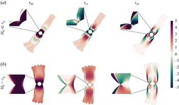
, including the rift tips, remains very large, while further away into the tongues region the flow becomes more uniform. These properties are particularly reflected in the stress field (figure 15). The hoop stress
 $\tau _{\theta \theta }$
in the interior region, including the rift tips and the vicinity of
 $r_g$
, exhibits pronounced extension, with values over one order of magnitude higher than in the tongues region. This indicates highly active interior azimuthal stretching (figure 15,
 $\tau _{\theta \theta }$
). The interior region also exhibits large compressive
 $\tau _{rr}$
that is more substantial when
 $H_0\ll r_g$
(figure 15,
 $\tau _{rr}$
). The weaker stress field along the tongues, far from the rifts region, is primarily extensional (
 $\tau _{\theta \theta }\gt 0,\tau _{rr}\gt 0$
), while an intermediate domain of compressional hoop stress arises when
 $H_0\ll r_g$
. The shear stress
 $\tau _{r\theta }$
nearly vanishes within the outer tongue regions, while near the rift tips it is substantially more intense. Unlike the normal stress components, the shear stress distribution is weakly dependent on the ratio
 $H_0/r_g$
(figure 15,
 $\tau _{r\theta }$
).
The exponent in the constitutive law,
 $n$
, has a critical effecton the stability (§ 4.3), as well as a quantitative effect on the stress field. This can be appreciated through the scalar fields, such as the second invariants of the stress and rate-of-strain tensors, and the fluid viscosity (figure 16). For
 $n = 0.5$
(shear-thickening regime), the front remains circular at late times (
 $t/T_k\gg 1$
), though memory of the initial perturbation wavenumber can persists for some time in the thickness field (e.g. figure 6
a). The stress and strain-rate invariants are axisymmetric, decay monotonically with radius, and despite the large perturbation amplitude (
 $A_0/\delta _0=0.5$
), have no apparent cusps (figure 16,
 $n=0.5$
). The corresponding viscosity also decreases gradually with radius and shows no variation along the front. As
 $n$
increases to
 $5.5$
and
 $9$
(shear-thinning regime), rifts emerge. Both the strain-rate and stress invariants have a local maximum at the rift tips, while the viscosity drops to minimum in that location (figure 16,
 $n=5.5,9$
). The rift-tips become increasingly local as
 $n$
grows, likely since the gradients of these fields grow with
 $n$
.
7. Conclusions
We have explored the stability of radially spreading extensional flows of power-law fluids, building on and extending the analysis of Newtonian extensional flows in Part 1 (Stern et al. Reference Stern, Gudmundsson and Sayag2025). Using numerical simulations of the SSA, we show that the spreading front becomes unstable to monochromatic perturbations as soon as the power-law exponent exceeds a critical threshold
 $n \approx 2$
, corresponding to a strain-rate softening (shear-thinning) fluid. Consequently, the initial axisymmetric flow evolves patterns consisting of tongues separated by active rifts. This marks a fundamental departure from the stable behaviour of Newtonian fluids, as well as the importance of the nonlinearity of the flow. Our results demonstrate that these fracture-like tearing patterns arise in a purely viscous, strain-rate softening fluid, involving no elasticity or damage mechanics.
Prior to the breakup of symmetry, our analysis shows that the radial distribution of the fluid mass is convex when the spreading is kinematically controlled, and concave when it is dynamically controlled. We also find that shortly after the perturbation, the simulated secondary flow and vorticity patterns are consistent with the theoretical predictions for a layer of uniform thickness. However, at later time the secondary flow and the dominant wavenumber divert from the predictions, though the cascade of the dominant wavenumber to a lower one is implied from the theory.
The instability and the emergence of non-axisymmetric patterns depend on the perturbation parameters and flow properties. The fluid exponent
 $n$
has the most dramatic effect on the stability. In particular, strain-rate hardening fluids (
 $n\lesssim 1$
) remain stable with possible cusp formation, as in Newtonian fluids (Part 1), while strain-rate softening fluids (
 $n\gt 1$
) are unstable. We find that the terminal dominant wavenumber of the patterns is weakly dependent of the initial wavenumber
 $k_0$
, while it grows with
 $n$
, with the perturbation relative amplitude
 $A_0/\delta _0$
, with the inverse of the initial width of the fluid layer
 $\delta _0$
, and when the early flow is kinematically dominated. The terminal dominant wavenumber is reached through coarsening of the dominant wavenumber over time, consistently with laboratory experiments and as implied from the theoretical analysis.
The instability mechanism can be partially described as a combination of a stabilising and destabilising radial forces operating at the front. The destabilising force is due to the shear-stress divergence, which grows with the hoop stress or azimuthal extension, independently of the nature of the fluid. In contrast, the stabilising force, which arises from the normal-stress divergence, declines the more strain-rate softening the fluid becomes. This mechanism is consistent with the theoretical prediction (Sayag & Worster Reference Sayag and Worster2019b ), yet it predicts only the signature of the maximum growth rate without the corresponding most-unstable wavenumber. Nevertheless, it provides a consistent interpretation of the numerical results and, in particular, the growing dominance of the destabilising force in developing active rifts.
We also identify the perturbation strain-rate second invariant,
 $E_{\textit{II}_1}$
as a useful predictor for the formation of active rifts in the simulations. Specifically, perturbation troughs are regions of positive
 $E_{\textit{II}_1}$
in shear thinning fluids, and consequently of more mobile fluid that facilitates the growth of troughs under azimuthal stretching. Those troughs that deepen faster involve larger deformation rates and correspondingly larger and more localised
 $E_{\textit{II}_1}$
. This turns the troughs’ minima sharper, with increasingly localised high stresses at the base of troughs, as also implied by the full stress second invariant. Consequently unstable troughs become gradually sharper, with cusp-like tips that grow into rifts.
The formation and evolution of rift patterns in radially spreading extensional flows are driven by a purely strain-rate softening (shear thinning) viscous mechanism. Our results strengthen the theoretical basis for interpreting front instabilities in polymeric solutions and in geophysical systems. Future work will focus on quantitative comparison to laboratory experiments (Sayag & Worster Reference Sayag and Worster2019a ) and interpretation of geophysical observation.
Acknowledgements
We thank Y. Ashkenazy for assisting with computational resources and G. H. Gudmundsson for helpful discussions on Úa.
Funding
LS is grateful to the Center for Integration in Science in the Ministry of Aliyah for financial support. This research was supported by the Israel Science Foundation (grant no. 3006/21).
Declaration of interests
The authors report no conflict of interest.


 r−θ
 r−z
 −z^
 n=9

 n=9
 k0=9
 δ0=0.3
 A0/δ0=1/2
 H0
 t=5,30

 Td/Tk
 n,A,Q
 H0
 Td/Tk≫1
 Td/Tk∼1
 Td/Tk≪1

 k0=7,δ0=0.3,A0/δ0=0.1
 n=9
 k=(π/2)/δ(t)
 k=7,2,1
 u1
 uII
 t/Tk=1.35

 n=0.5,1.3,4
 n⩽1
 n>1
 n=6
 θ≈0
 n=6
 θ≈0,π
 θ≈0
 k0=9
 δ0=0.3
 A0/δ0=1/2
 A
 n>1
 n=0.5

 k0=3,4
 n=9
 δ0=0.3
 A0/δ0=0.5
 A0/δ0=0.3

 n,δ0
 kmax
 n
 δ(t)
 n≲2
 n≳2
 k=1
 n<7
 k=2
 n⩾7
 n
 n

 a0≃0
 a0=0.1
 n=9
 δ0=0.3
 a0=0.1,0.5
 k0=9

 A0=0.15
 δ0=0.16,0.2,0.4
 n=9
 k0=9

 H0/rg≪1
 Td≈100
 Q,Q/12,Q/60
 Tk≈0.7,9.3,46.5
 n=9,δ0=0.3
 a0=0.8
 k0=9

 H0/rg∼1
 Td≈10−5
 2Q,Q,Q/10
 Tk≈2.2,4.4,44.1
 n=9,δ0=0.3
 A0/δ0=0.8
 k0=9

 n=9
 k0=9
 δ0=0.3
 F1D,F1S,−∂p1/∂r
 EII1
 k=5
 k0=9
 A0/δ0=0.1
 t/Tk=0.45,0.9,1.35

 n=9
 k0=9
 δ0=0.3
 A0/δ0=0.5
 FD,FS,−∂p/∂r
 EII
 t/Tk=0.45,0.9,1.35
 n=9
 k0=9
 δ0=0.3
 A0/δ0=0.5
 H0≪rg
 H0∼rg

 n=0.5
 n=5.5
 n=9
 τII
 η
 EII
 k0=9
 δ0=0.3
 A0/δ0=0.5
 n=0.5
 A=9.7×10⁻⁵
 −n
 −1
 n>1
 A=9.7×10⁻⁹
 −n
 −1

 Open access

