1 Introduction
In the last two decades, the research of wall-bounded shear flows has revealed the existence of very large-scale elements that are an order of magnitude or more longer than the characteristic vertical flow dimension
 $\unicode[STIX]{x1D6FF}$
(Jiménez Reference Jiménez1998; Kim & Adrian Reference Kim and Adrian1999). Due to their extraordinarily large dimensions, these motions are termed very-large-scale motions (VLSMs) (Kim & Adrian Reference Kim and Adrian1999; Hambleton, Hutchins & Marusic Reference Hambleton, Hutchins and Marusic2006) or global modes (Del Alamo et al.
Reference Del Alamo, Jiménez, Zandonade and Moser2004) in internal flows, and superstructures (Hutchins & Marusic Reference Hutchins and Marusic2007) in external flows. These very-large-scale features, VLSMs from now on, have also large transverse dimensions of the order of
 $\unicode[STIX]{x1D6FF}$
(Hutchins & Marusic Reference Hutchins and Marusic2007). VLSMs are dynamically significant motions, which bear significant fractions of kinetic energy, and Reynolds shear stress (del Álamo & Jiménez Reference del Álamo and Jiménez2003; Del Alamo et al.
Reference Del Alamo, Jiménez, Zandonade and Moser2004; Guala, Hommema & Adrian Reference Guala, Hommema and Adrian2006; Lee & Sung Reference Lee and Sung2011).
The dynamical significance of VLSMs becomes more pronounced with increasing Reynolds numbers (Smits, McKeon & Marusic Reference Smits, McKeon and Marusic2011). In this regard, VLSMs are also found to exist in the atmospheric boundary layer (ABL) (Kunkel & Marusic Reference Kunkel and Marusic2006; Hutchins et al.
Reference Hutchins, Chauhan, Marusic, Monty and Klewicki2012; Wang & Zheng Reference Wang and Zheng2016), where the friction Reynolds number
 $Re_{\unicode[STIX]{x1D70F}}$
is in the range
 $O(10^{6}{-}10^{7})$
. To date, the role of these very-large-scale energetic motions on wind-energy harvesting is not explored. In this study, we numerically investigate how VLSMs and associated flow structures redistribute their momentum and energy when they encounter a row of wind turbines parallel to them. In particular, we will make an attempt to elucidate the influence of VLSMs on some flow properties of interest, e.g. the dominance of turbulent momentum transport in lateral directions around the turbine row and large-scale streamwise velocity fluctuations in the turbine wakes.
1.1 General characteristics of VLSMs
VLSMs are classified as energetic motions with streamwise scales
 $O(10\unicode[STIX]{x1D6FF})$
and spanwise scales
 $O(\unicode[STIX]{x1D6FF})$
(Marusic et al.
Reference Marusic, McKeon, Monkewitz, Nagib, Smits and Sreenivasan2010). Instantaneous fields of streamwise velocity showed that these motions are in the form of coherent meandering streaks with lengths reaching
 $20\unicode[STIX]{x1D6FF}$
in boundary layers (Hutchins & Marusic Reference Hutchins and Marusic2007), or
 $30\unicode[STIX]{x1D6FF}$
in internal flows (Lee & Sung Reference Lee and Sung2011). Being the largest scales of the flow, VLSMs are affected by the boundary conditions, and show slightly different characteristics in different flows (Monty et al.
Reference Monty, Hutchins, Ng, Marusic and Chong2009). In this regard, the very long streaks in boundary layers are more prominent in the inertial layer and lower wake region (Hutchins & Marusic Reference Hutchins and Marusic2007), while in internal flows they extend to the whole layer (Monty et al.
Reference Monty, Stewart, Williams and Chong2007). Very long streaks also penetrate to the near-wall layer (Metzger & Klewicki Reference Metzger and Klewicki2001; Hoyas & Jiménez Reference Hoyas and Jiménez2006), and have nonlinear interactions with much smaller scales there (Mathis, Hutchins & Marusic Reference Mathis, Hutchins and Marusic2009).
The mechanical origin of very long streaks, and the dynamics behind their high Reynolds stress content remains an unresolved issue. For sufficiently high Reynolds numbers, these outer-scale motions coexist in the inertial layer with another dynamically important class of motions with an inner scaling, i.e. Townsend’s attached eddies (Townsend Reference Townsend1976). These eddies build a self-similar hierarchy where each element scales with its distance to the wall (
 $z$
), and they are associated with the
 $k_{x}^{-1}$
range in the streamwise wavenumber spectrum (Marušić & Perry Reference Marušić and Perry1995). The top elements of the hierarchy reach length scales of
 $O(\unicode[STIX]{x1D6FF})$
(Perry, Henbest & Chong Reference Perry, Henbest and Chong1986), and belong to the class of large-scale motions (LSMs), cf. Marusic et al. (Reference Marusic, McKeon, Monkewitz, Nagib, Smits and Sreenivasan2010) for a discussion of these motions.
Various attempts have been made to reveal the time-resolved kinematic identity of the inertial-layer motions. Khanna & Brasseur (Reference Khanna and Brasseur1998) showed that the streamwise-velocity field in the inertial layer of shear-dominated ABL organizes into low-speed streaks. They suggested that the streaks are produced by the local shear, as similar streaks are also observed in the absence of the wall in homogenous shear turbulence, cf. Lee, Kim & Moin (Reference Lee, Kim and Moin1990). Adrian and coworkers associated streaks with the hairpin vortex paradigm, and suggested that long streaks are signatures of hairpin vortex packets (Adrian, Meinhart & Tomkins Reference Adrian, Meinhart and Tomkins2000; Tomkins & Adrian Reference Tomkins and Adrian2003). However, other researchers did not observe hairpin forms, and reported more disorganized shell-like elements arranged as wall-attached vortex clusters (Del Álamo et al. Reference Del Álamo, Jimenez, Zandonade and Moser2006) or sweep ejection surfaces (Lozano-Durán, Flores & Jiménez Reference Lozano-Durán, Flores and Jiménez2012). All these reported structures have statistical properties similar to Townsend’s attached eddies. The relation of these motions to VLSMs is not clear. Whether the very long streaks emerge from an ‘inverse cascade’ through alignment of hairpin vortex packets (Adrian Reference Adrian2007; Lee & Sung Reference Lee and Sung2011), or in contrast, by a top–down mechanism originating from outer-layer fluctuations (Högström, Hunt & Smedman Reference Högström, Hunt and Smedman2002), or rather by global linear processes (Del Álamo & Jimenez Reference Del Álamo and Jimenez2006; Hwang & Cossu Reference Hwang and Cossu2010; McKeon & Sharma Reference McKeon and Sharma2010), is the subject of ongoing research.
Hutchins et al. (Reference Hutchins, Chauhan, Marusic, Monty and Klewicki2012) studied geometrical features of VLSMs using conditional analysis on pointwise negative velocity events. They obtained
 $\unicode[STIX]{x1D6FF}$
-scale streamwise vortex pairs accompanying very long low-momentum regions (streaks) that are flanked on both sides by high-momentum regions. These statistical streaks are somewhat shorter than their instantaneous counterparts due to meandering tendency of the latter (Hutchins & Marusic Reference Hutchins and Marusic2007). The structure is inclined towards streamwise direction by an angle of approximately
 $14^{\circ }$
, and this inclination angle is found to be insensitive to Reynolds number (Marusic & Heuer Reference Marusic and Heuer2007). Similar streak–roller structures are also observed by Del Álamo et al. (Reference Del Álamo, Jimenez, Zandonade and Moser2006) using a vortex-based conditional analysis, and by Hwang (Reference Hwang2015) using scale-isolating large-eddy simulations (LESs). In these studies, the structure is paired to another LSM-sized feature. The topology of the streak–roller structure provides some insight into the high Reynolds stress content in VLSMs, as low and high-streamwise-velocity regions are associated with updrafts and downdrafts respectively. The form is reminiscent of buffer-layer streaks and counter-rotating vortices (Robinson Reference Robinson1991). However, it is
 $O(Re_{\unicode[STIX]{x1D70F}}/10)$
times larger, and its dynamics is entangled to many other scales in the outer layer. To study the dynamics of very-large-scale streak–rollers in a more comprehensible framework, various researchers used simplified forms of the Navier–Stokes equations, cf. e.g. Farrell et al. (Reference Farrell, Ioannou, Jiménez, Constantinou, Lozano-Durán and Nikolaidis2016).
1.2 VLSMs in the atmospheric boundary layer
VLSMs and associated
 $\unicode[STIX]{x1D6FF}$
-scale streak–roller structures (with
 $\unicode[STIX]{x1D6FF}$
the thickness of the atmospheric surface layer) are also ubiquitous in the atmospheric surface layer in near-neutral conditions (Hutchins et al.
Reference Hutchins, Chauhan, Marusic, Monty and Klewicki2012). Chauhan et al. (Reference Chauhan, Hutchins, Monty and Marusic2013) showed that very long regions of positive correlation in the streamwise direction also exist in the presence of buoyancy forces. In unstable buoyancy conditions, the structures are larger and steeper with an inclination angle of up to
 $34^{\circ }$
. The inclination angle is increased by the vertical lifting of buoyancy forces (Carper & Porté-Agel Reference Carper and Porté-Agel2004), and its value depends on the relative magnitude of the heat flux. In stably stratified conditions, Chauhan et al. (Reference Chauhan, Hutchins, Monty and Marusic2013) further showed that the extent of the streamwise correlation is slightly shorter than its counterpart in neutral or unstable conditions, and it is limited to a thin layer near the surface. Above this thin layer, there are large regions of negative correlation. These variations in the topology suggest a significantly different mechanism responsible for large-scale coherence in stable conditions.
Modern wind turbines, with their dimensions reaching 100 metres, occupy almost the entire surface layer of the ABL. Therefore, in asymptotically large wind farm conditions, they are expected to disintegrate large-scale ABL elements in the surface layer. In this context, large-scale structures that extend beyond the surface layer, e.g. occupying the entire ABL, are of more practical interest for wind-energy harvesting. The existence of such features is long known in the unstably stratified ABL, and they are denoted roll vortices in the meteorological literature, cf. Etling & Brown (Reference Etling and Brown1993), Young et al. (Reference Young, Kristovich, Hjelmfelt and Foster2002). However, these structures are considered to be different in nature than VLSMs in canonical boundary layers (Hutchins et al. Reference Hutchins, Chauhan, Marusic, Monty and Klewicki2012), as the effect of buoyancy forces is very prominent above the surface layer (Moeng & Sullivan Reference Moeng and Sullivan1994; Khanna & Brasseur Reference Khanna and Brasseur1998).
Fang & Porté-Agel (Reference Fang and Porté-Agel2015) showed the existence of very large ABL-scale features in shear-driven ABL using cross-correlation maps in their LES data. They found that the streamwise velocity is correlated across the whole ABL, and the VLSM-sized streaks are accompanied by counter-rotating rollers. Shah & Bou-Zeid (Reference Shah and Bou-Zeid2014) studied VLSMs in the presence of the buoyancy and Coriolis forces using LES and proper orthogonal decomposition (POD). They found that
 $\unicode[STIX]{x1D6FF}$
-scale (
 $\unicode[STIX]{x1D6FF}$
is the ABL thickness) streamwise rollers with a vertical tilting from
 $0^{\circ }$
to
 $30^{\circ }$
due to Ekman turning are the dominant modes under neutrally stratified conditions. They also showed that these very-large-scale structures change their character in the presence of the strong buoyant plumes, and do not exist in stably stratified conditions.
In wind-energy context, very long persistent streaks in pressure-driven wind farm boundary-layer simulations provide evidence for VLSMs in densely populated wind farms under neutrally stratified conditions, cf. Munters, Meneveau & Meyers (Reference Munters, Meneveau and Meyers2016a ). These streaks extend to the entire domain in the streamwise and vertical direction, and penetrate also to the regions between the turbine rows. They are long lived, i.e. they endure the effects of turbines and their dynamic meandering wakes. Therefore, these structures are a major dynamic component of wind farm boundary layers. VerHulst & Meneveau (Reference VerHulst and Meneveau2014) conducted POD analysis of a similar pressure-driven wind farm boundary layer under neutral conditions, and identified a hierarchy of two-dimensional streak–roller structures. The top elements of the hierarchy contained streamwise rollers spanning the entire ABL. These essentially two-dimensional modes are rather a consequence of periodicity of the simulation box.
1.3 The scope of the work
Besides the obvious low-frequency power fluctuations, VLSMs are expected to play a dual role in wind-energy harvesting. Their large circulatory fields can enhance the momentum exchange between the turbine wakes and atmosphere, and increase the efficiency of densely populated wind farms. On the other hand, these energetic motions may drive the turbine wakes towards transverse directions, and enhance the eccentric loading of turbine components. The goal of this study is to exploit the links between these effects and the morphology of VLSMs using a simple setting: a turbine row aligned to the flow direction operating under neutrally stratified conditions. To this end, we perform simulations of a neutral pressure-driven boundary layer, neglecting effects of Coriolis forces and free-atmosphere stratification, and using a simple symmetry boundary condition at the top of our simulation domain. First of all, we remark here that ABL-scale VLSMs are particular for neutral boundary layers – they do not exist above the surface layer of stable boundary layers, and change in nature in unstable boundary layers, cf. Shah & Bou-Zeid (Reference Shah and Bou-Zeid2014). Although stable and unstable BLs are more common over land, the study of neutral boundary layers is nevertheless quite relevant, as they do occur quite often over sea (see, e.g. Brost, Lenschow & Wyngaard Reference Brost, Lenschow and Wyngaard1982; Grant Reference Grant1986; Tjernström & Smedman Reference Tjernström and Smedman1993). Secondly, in the atmosphere, truly neutral boundary layers almost never occur. In reality, neutral boundary layers are always of the conventionally neutral type, in which the neutral ABL is capped by a strongly stable inversion layer, and stable free atmosphere above. These impose complex boundary conditions on the outer layer of the boundary layer that include strong temperature gradients and wind veer. However, these effects remain located relatively close to the capping inversion itself, and for boundary layers that are sufficiently high, the surface layer, turbine region and logarithmic layer are to first order unaffected. Therefore neutral ABLs are very often represented with a simple pressure-driven boundary layer, and this is also a standard approach in LES of large wind farms, e.g. Calaf, Meneveau & Meyers (Reference Calaf, Meneveau and Meyers2010), Calaf, Parlange & Meneveau (Reference Calaf, Parlange and Meneveau2011), Wu & Porté-Agel (Reference Wu and Porté-Agel2013). For instance, Allaerts & Meyers (Reference Allaerts and Meyers2018) presented a comparison between a simple pressure-driven boundary layer and a boundary layer with a capping inversion at 500 m, showing that velocity and stress profiles collapse up to 300 m. In the current manuscript, we consider a boundary layer with a height of
 $\unicode[STIX]{x1D6FF}=1000~\text{m}$
, so that the use of a pressure-driven boundary layer is a reasonable approach, that much simplifies our simulation set-up.
The extraordinarily large dimensions of VLSMs cause two essential issues in a computational domain with periodic boundaries. First, a portion of the overall turbulent kinetic energy may not be represented due to finite streamwise extent of the domain. This effect is evident in the premultiplied spectrum of streamwise fluctuations, e.g. Hoyas & Jiménez (Reference Hoyas and Jiménez2006) showed for a moderate Reynolds number channel flow that contours remain open in the longest streamwise wavelength (
 $\unicode[STIX]{x1D706}_{x}$
) range. Lozano-Durán & Jiménez (Reference Lozano-Durán and Jiménez2014) later managed to close these contours at
 $\unicode[STIX]{x1D706}_{x}\approx 100\unicode[STIX]{x1D6FF}$
by conducting the simulation in a very long domain of
 $L_{x}=60\unicode[STIX]{x03C0}\unicode[STIX]{x1D6FF}$
. The second issue, which is especially important in wind farm simulations, is the stabilizing effect of periodicity on the VLSMs that occupy the entire streamwise extend, i.e. motions corresponding to wavenumbers
 $k_{x}=0,k_{y}\neq 0$
. These VLSMs are very stable structures, and appear to have very long lifetime, which inhibits the spatial chaos of large-scale motions, and yields unnatural inhomogeneities in channel flow (Fishpool, Lardeau & Leschziner Reference Fishpool, Lardeau and Leschziner2009) and wind farm (Munters et al.
Reference Munters, Meneveau and Meyers2016a
) simulations. This artificial effect of periodicity also increases the statistical dimensions of VLSMs, and make them significantly longer than the reported values in experiments, e.g. Liu, Wang & Zheng (Reference Liu, Wang and Zheng2017) for a recent study about the statistical size of VLSMs. In order to minimize these artefacts and represent very-large scales of
 $O(10\unicode[STIX]{x1D6FF})$
realistically in the current work, ABL data are produced in a separate domain that has a streamwise extend of
 $240\unicode[STIX]{x1D6FF}$
.
The diameter of the wind turbines is
 $D=100~\text{m}=0.1\unicode[STIX]{x1D6FF}$
, and they are placed
 $z_{h}=100~\text{m}=0.1\unicode[STIX]{x1D6FF}$
above the ground. Due to the excessive cost of representing turbine blades and associated finer-scale turbulent flow structures on a LES grid, these flow features are usually not resolved, and the forces they impose on the boundary layer are modelled. To this end, several turbine models with varying degrees of sophistication exist. A common approach in this regard is the actuator–disk model (ADM) (Jimenez et al.
Reference Jimenez, Crespo, Migoya and Garcia2007), where turbines are considered to impose uniform axial forces over a rotor disk. This simple drag model can reproduce realistic turbulent statistics especially in the far wake (Meyers & Meneveau Reference Meyers and Meneveau2010), and has been a standard workhorse in numerous wind farm boundary-layer studies, e.g. Calaf et al. (Reference Calaf, Meneveau and Meyers2010, Reference Calaf, Parlange and Meneveau2011), Goit & Meyers (Reference Goit and Meyers2015). ADM is also the method of choice in the current work.
We study VLSMs by filtering out our LES database at a streamwise cutoff wavelength
 $\unicode[STIX]{x1D706}_{x}=5\unicode[STIX]{x1D6FF}=50D$
. Statistics of the filtered fields reveal very long wake-like components around the turbines, which contain approximately
 $20\,\%$
of the resolved Reynolds shear stress, and
 $30\,\%$
of the resolved streamwise kinetic energy. In order to analyse the role of very-large-scale turbulent structures on the development of these statistics, we extract the statistical geometry of VLSMs using one-point conditional averaging based on low-pass filtered streamwise-velocity events. To this end, we select various points around the turbine row and far in the ABL at
 $z=0.15$
, and
 $z=0.45\unicode[STIX]{x1D6FF}$
.
The paper is organized as follows. First, the computational details and flow configuration are described in § 2. Then, the characteristics of the turbulent transport around the turbine row are investigated in § 3. Subsequently, we will study the filtered fields in § 4, and the streak–roller structures in § 5. Finally, the results are summarized in § 6.
2 Numerical details
2.1 Governing equations and their discretization
We consider LES of a thermally neutral ABL, which is driven using a constant pressure gradient. We use a Cartesian coordinate system where
 $x$
,
 $y$
,
 $z$
correspond to streamwise, spanwise and wall-normal directions associated with unit vectors
 $\hat{\boldsymbol{e}}_{x}$
,
 $\hat{\boldsymbol{e}}_{y}$
and
 $\hat{\boldsymbol{e}}_{z}$
, respectively. The governing equations are the filtered momentum and continuity equations for incompressible flows
 $$\begin{eqnarray}\displaystyle & \displaystyle \frac{\unicode[STIX]{x2202}\widetilde{\boldsymbol{u}}}{\unicode[STIX]{x2202}t}+\widetilde{\boldsymbol{u}}\boldsymbol{\cdot }\unicode[STIX]{x1D735}\widetilde{\boldsymbol{u}}=-\frac{1}{\unicode[STIX]{x1D70C}}\unicode[STIX]{x1D735}\widetilde{p}+\unicode[STIX]{x1D735}\boldsymbol{\cdot }\unicode[STIX]{x1D749}^{R}+f_{\infty }\hat{\boldsymbol{e}}_{x}+\boldsymbol{f}_{t}, & \displaystyle\end{eqnarray}$$
 $$\begin{eqnarray}\displaystyle & \displaystyle \unicode[STIX]{x1D735}\boldsymbol{\cdot }\widetilde{\boldsymbol{u}}=0, & \displaystyle\end{eqnarray}$$
where
 $\widetilde{\boldsymbol{u}}=[\widetilde{u}_{x},\widetilde{u}_{y},\widetilde{u}_{z}]$
is the resolved velocity field,
 $\widetilde{p}$
is the resolved pressure field excluding the driving pressure gradient embedded into
 $f_{\infty }$
,
 $\unicode[STIX]{x1D70C}$
is the uniform constant density,
 $\unicode[STIX]{x1D749}^{R}$
are the subgrid-scale stresses (SGS) and
 $\boldsymbol{f}_{t}$
represent the drag forces imposed on the flow by turbines. The resolved viscous stresses are neglected, as the considered rough-wall model (see the discussion below) allows the first grid point of the bottom boundary to be in the inertial layer, where the resolved viscous effects are negligibly small due to very high Reynolds number of the ABL. Throughout the paper,
 $[\langle \widetilde{u}_{x}\rangle ,\langle \widetilde{u}_{y}\rangle ,\langle \widetilde{u}_{z}\rangle ]$
represent the components of mean resolved velocity
 $\langle \widetilde{\boldsymbol{u}}\rangle$
, and
 $[\widetilde{u}_{x}^{\prime },\widetilde{u}_{y}^{\prime },\widetilde{u}_{z}^{\prime }]$
are the fluctuating parts. We will use the friction velocity
 $u_{\ast }=(f_{\infty }\unicode[STIX]{x1D6FF}/\unicode[STIX]{x1D70C})^{1/2}$
to scale dynamic quantities.
The filtered equations are discretized and solved using the in-house research code SP-Wind. SP-Wind has been previously employed in a series of wind-energy applications under neutral conditions, e.g. Calaf et al. (Reference Calaf, Meneveau and Meyers2010), Meyers & Meneveau (Reference Meyers and Meneveau2013), Allaerts & Meyers (Reference Allaerts and Meyers2015a ), Goit & Meyers (Reference Goit and Meyers2015). Moreover, validation and comparison studies can be found in Munters, Meneveau & Meyers (Reference Munters, Meneveau and Meyers2016b ) and Lignarolo et al. (Reference Lignarolo, Mehta, Stevens, Yilmaz, van Kuik, Andersen, Meneveau, Ferreira, Ragni and Meyers2016). The reader is referred to these works for the details of the numerical methods, SGS, turbine and roughness models. Here we will briefly review them for completeness.
We employ a classical Smagorinsky (Reference Smagorinsky1963) model with constant coefficient
 $C_{s}=0.14$
to model the subgrid-scale stresses. A wall damping is applied in the vicinity of the bottom boundary where the Smagorinsky length
 $l$
(
 $=C_{s}(\unicode[STIX]{x0394}x\unicode[STIX]{x0394}y\unicode[STIX]{x0394}z)^{1/3}$
away from the wall) is reduced using the wall damping function of Mason & Thomson (Reference Mason and Thomson1992).
Periodic boundary conditions are employed in the streamwise and spanwise directions. Symmetry conditions are applied at the top boundary. At the bottom boundary, a no-penetration boundary condition is imposed for the vertical component of the velocity
 $\widetilde{u}_{z}$
. In the tangential directions a wall stress model is applied, which relates the wall stress to the tangential components of the velocity at the first grid point using the law of the wall (Bou-Zeid, Meneveau & Parlange Reference Bou-Zeid, Meneveau and Parlange2005):
 $$\begin{eqnarray}\displaystyle & \displaystyle \unicode[STIX]{x1D70F}_{wx}(x,y)=-\left(\frac{\unicode[STIX]{x1D705}}{\text{ln}(z_{1}/z_{0})}\right)^{2}(\widehat{\widetilde{u}}_{x}(x,y,z_{1})^{2}+\widehat{\widetilde{u}}_{y}(x,y,z_{1})^{2})^{0.5}\widehat{\widetilde{u}}_{x}(x,y,z_{1}), & \displaystyle\end{eqnarray}$$
 $$\begin{eqnarray}\displaystyle & \displaystyle \unicode[STIX]{x1D70F}_{wy}(x,y)=-\left(\frac{\unicode[STIX]{x1D705}}{\text{ln}(z_{1}/z_{0})}\right)^{2}(\widehat{\widetilde{u}}_{x}(x,y,z_{1})^{2}+\widehat{\widetilde{u}}_{y}(x,y,z_{1})^{2})^{0.5}\widehat{\widetilde{u}}_{y}(x,y,z_{1}), & \displaystyle\end{eqnarray}$$
where
 $z_{0}$
is the surface roughness parameter,
 $z_{1}$
is the height of the first grid point and
 $\widehat{(\cdot )}$
operator represents a local average obtained by filtering in wall-parallel directions.
A pseudo-spectral discretization is applied in the horizontal directions. The nonlinear convective terms, and SGS stress are dealiased using the
 $2/3$
rule (Boyd Reference Boyd2001). A fourth-order energy conservative finite-difference discretization is applied in the wall-normal direction (Verstappen & Veldman Reference Verstappen and Veldman2003). Time stepping is achieved using a fourth-order four-stage Runge–Kutta scheme.
The forces imposed by the turbines are modelled using a standard actuator–disk method (Jimenez et al.
Reference Jimenez, Crespo, Migoya and Garcia2007). In this model, turbines are considered to impose uniform axial forces over a rotor disk with a diameter
 $D$
. In our configuration, the turbines are aligned with the streamwise direction
 $\hat{\boldsymbol{e}}_{x}$
, and the force field imposed by each turbine reads in this configuration as follows
 $$\begin{eqnarray}\boldsymbol{f}_{t}^{i}(\boldsymbol{x},t)=-{\textstyle \frac{1}{2}}C_{T,i}\overline{V_{i}}(t)^{2}\mathscr{R}_{i}(\boldsymbol{x})\hat{\boldsymbol{e}}_{x},\end{eqnarray}$$
where
 $C_{T,i}$
is a constant disk-based thrust coefficient with a selected value of
 $4/3$
(similar to Calaf et al.
Reference Calaf, Meneveau and Meyers2010),
 $\overline{V_{i}}(t)$
is the axial flow velocity averaged over the rotor disk,
 $\mathscr{R}_{i}(\boldsymbol{x})$
is the smoothing function to project the calculated forces on LES grid (Meyers & Meneveau Reference Meyers and Meneveau2010), it is by construction
 $\int _{\unicode[STIX]{x1D6FA}}\mathscr{R}_{i}(\boldsymbol{x})\,\text{d}\boldsymbol{x}^{\prime }=\unicode[STIX]{x03C0}D^{2}/4$
. The sum of all turbine forces equals to
 $\boldsymbol{f}_{t}$
in (2.1), i.e.
 $\boldsymbol{f}_{t}=\sum \boldsymbol{f}_{t}^{i}$
. Finally, we remark that many variants of the ADM exist, and in particular some versions include effects of rotation (Meyers & Meneveau Reference Meyers and Meneveau2010; Wu & Porté-Agel Reference Wu and Porté-Agel2011). These have been shown to be important to correctly represent near-wake details (Wu & Porté-Agel Reference Wu and Porté-Agel2011), but effects of rotation are negligible in the far wake and on the larger scale (Wu & Porté-Agel Reference Wu and Porté-Agel2011; Meyers & Meneveau Reference Meyers and Meneveau2013). Thus we do not expect effects of rotation to be critical when studying the interaction between turbine wakes and very-large-scale motions. Nevertheless, the use of alternative turbine models such as rotating ADM or actuator line models may be an interesting topic for future research.
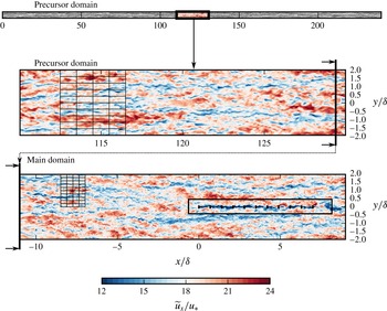
2.2 A two-grid approach
The two-grid methodology is demonstrated using planes at hub height, i.e.
 $z=0.1\unicode[STIX]{x1D6FF}$
. ABL data are first produced separately in a very long precursor domain of
 $240\unicode[STIX]{x1D6FF}$
using a moderate grid resolution. The data are mapped then to the main domain where turbines are located
 $11\unicode[STIX]{x1D6FF}$
downstream to allow cascade between the two cutoff scales. Representative computational grids are shown using every fifteenth point in each direction. A fringe region (not shown here) is employed to apply the streamwise periodicity in the main domain.

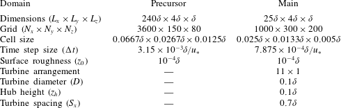
Domain and grid specifications for two-grid approach.
 $\unicode[STIX]{x1D6FF}$
is the thickness of the atmospheric boundary layer.

In order to study VLSMs in a realistic setting within an affordable computational cost, we employ a two-grid approach. The method is demonstrated in figure 1, and the domain and grid specifications are summarized in table 1. The strategy is not a simultaneous one, and is based on two separate steps. We first simulate the neutrally stratified ABL in a very long domain of
 $240\unicode[STIX]{x1D6FF}$
using a moderate grid resolution. During this precursor simulation, a database of inflow planes is constructed using a transverse
 $y$
–
 $z$
plane at a selected streamwise location. Then, the inflow data are mapped to the main domain. As the main domain contains a higher grid resolution, a second-order spatial interpolation is employed in this process. The first two rows near the ground on the fine grid remain exterior to the coarse grid. At these exterior points, we employed a second-order extrapolation from neighbouring points at higher altitudes. As an alternate, we also tested higher-order interpolations and a more complicated extrapolation taking the logarithmic variation of the streamwise-velocity component into account. However, we found the convergence in the main domain to be only marginally effected.
We employed a fixed time step size (
 $\unicode[STIX]{x0394}t$
) for both simulations. In the precursor domain
 $\unicode[STIX]{x0394}t=3.15\times 10^{-3}\unicode[STIX]{x1D6FF}/u_{\ast }$
corresponding to a maximum Courant–Friedrichs–Lewy (CFL) number of approximately 0.7, and in the main domain
 $\unicode[STIX]{x0394}t=7.875\times 10^{-4}\unicode[STIX]{x1D6FF}/u_{\ast }$
corresponding to a maximum CFL number of approximately 0.4. As time steps in both simulations are different, we also employed a second-order interpolation in time in the mapping process.
The periodicity on the main domain is circumvented using a fringe region approach in which an additional force is applied to bring the actual flow to the desired values given by the inflow data. Details of the fringe region method can be found in Munters et al. (Reference Munters, Meneveau and Meyers2016b
). In the original method, Munters et al. (Reference Munters, Meneveau and Meyers2016b
) employed three-dimensional slab data for the forcing function to prevent Gibbs oscillations. As mentioned above, we have used two-dimensional planar data for fringe forcing. The upstream influence of sharp transition due to two-dimensional forcing were found to be limited to only a few
 $\unicode[STIX]{x1D6FF}$
from the fringe region. Moreover, in our test with three-dimensional slabs, we did not notice any improvement in the transition in the main domain. Consequently, planar mapping is selected to reduce the storage costs.
The configuration for turbine size, height and horizontal spacing is the same as in the earlier work of Goit & Meyers (Reference Goit and Meyers2015). The diameter of the turbines is
 $D=0.1\unicode[STIX]{x1D6FF}$
. The 11 turbines are aligned in the streamwise direction with a spacing of
 $S_{x}=0.7\unicode[STIX]{x1D6FF}$
, and their hub height is at
 $z_{h}=0.1\unicode[STIX]{x1D6FF}$
. The location of the first turbine centre is at
 $x=0$
,
 $y=0$
,
 $z=0.1\unicode[STIX]{x1D6FF}$
. Finally, the last
 $1.75\unicode[STIX]{x1D6FF}$
of the main domain is used as fringe region. The last turbine is
 $5.25\unicode[STIX]{x1D6FF}$
away from the fringe region. As cutoff scales are different on precursor and main domains, the turbine row is placed at
 $11\unicode[STIX]{x1D6FF}$
downstream from the entrance boundary to allow a cascade to develop between the two cutoff scales. The statistics of this transition are elaborated in § 2.3.
For the analysis of the flow, we have saved approximately
 $10\,000$
three-dimensional snapshots that are separated in time by
 $0.0315\unicode[STIX]{x1D6FF}/u_{\ast }$
. Consequently, the database covers a convection length of approximately
 $5500\unicode[STIX]{x1D6FF}$
at hub height. In the following sections, averaging over the symmetry half-plane
 $y=0$
is employed whenever possible.
2.3 Analysis of the transition in the main domain
Evolution of turbulent quantities in the transition region of the main domain
 $x/\unicode[STIX]{x1D6FF}<-1$
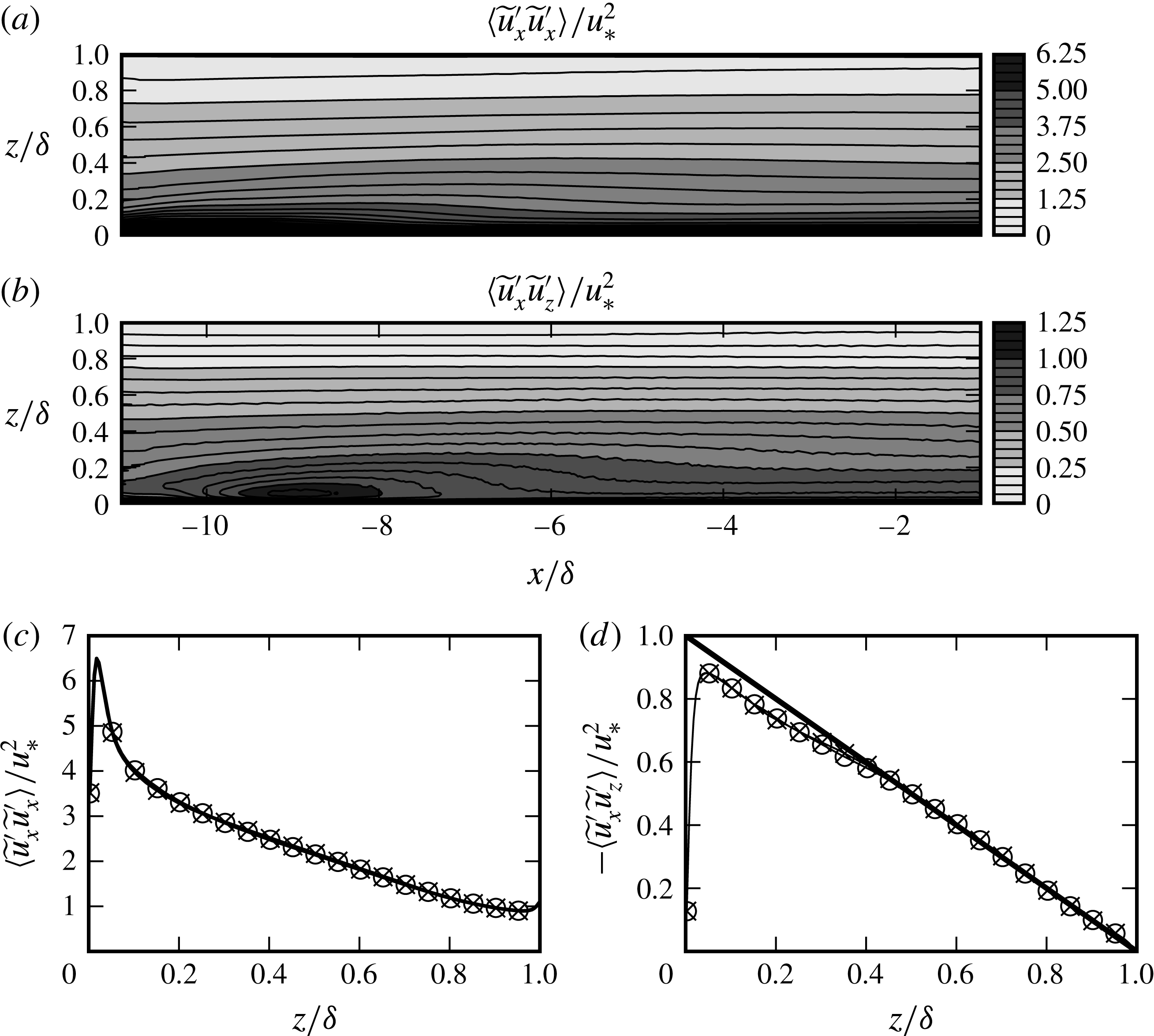
. Filled contours show the resolved normal Reynolds stress, and Reynolds shear stress. (c,d) Show vertical variation of these stresses; (——
 $\times$
)
 $x/\unicode[STIX]{x1D6FF}=-2.5$
and (——○)
 $x/\unicode[STIX]{x1D6FF}=-1$
. The solid line in (d) represents
 $\unicode[STIX]{x1D70F}(z)=1-z/\unicode[STIX]{x1D6FF}$
.

Figure 2(a,b) shows the evolution of the resolved normal stress
 $\langle \widetilde{u}_{x}^{\prime }\widetilde{u}_{x}^{\prime }\rangle$
and the resolved tangential stress
 $-\langle \widetilde{u}_{x}^{\prime }\widetilde{u}_{z}^{\prime }\rangle$
in the transition region
 $x/\unicode[STIX]{x1D6FF}<-1$
, where the flow is assumed to be homogeneous in the spanwise direction. We see that in the first
 $7\unicode[STIX]{x1D6FF}$
from the inflow (
 $x/\unicode[STIX]{x1D6FF}<-4$
), there is a strong transition with overshoots in both quantities, especially noticeable for
 $z/\unicode[STIX]{x1D6FF}<0.2$
. At
 $x/\unicode[STIX]{x1D6FF}\approx -2.5$
, the contour lines become approximately horizontal suggesting that the transition of the ABL data from coarse grid to fine one is accomplished. This can also be seen in the vertical profiles of the stresses at
 $x=-2.5\unicode[STIX]{x1D6FF}$
and
 $x=-\unicode[STIX]{x1D6FF}$
, cf. figure 2(c,d). However, we see in figure 2(d) that the shear stress profile at the end of the transition region has a slight deviation for
 $z/\unicode[STIX]{x1D6FF}\leqslant 0.4$
from the
 $-1$
slope that can be expected in a homogeneous boundary layer in balance. Note that in figure 2(d) only the resolved stresses are represented. However, in our simulations, the contributions of the mean subgrid-scale stress to the total shear stress are negligible for
 $z>0.1\unicode[STIX]{x1D6FF}$
. The discrepancy in the momentum balance is induced by a slow transition of the mean fields, which is caused by an inevitable slight grid sensitivity of the LES approach. When the coarse grid fields are fed into the fine grid domain, the mean fields evolve into a slightly modified equilibrium in the surface layer. This is a slow process, which would require a very long fetch to complete, so that it is computationally not feasible to re-equilibrate the mean flow with a longer main domain. At
 $x/\unicode[STIX]{x1D6FF}=-1$
, we observe an error of
 $5\,\%$
on the wall stress, which leads to a slightly accelerating flow, and a small vertical mean-flow component, which peaks at approximately
 $z/d\approx 0.2$
with a value of
 $\langle \widetilde{u}_{z}\rangle \approx 0.005u_{\ast }$
. However, since this imbalance is small, we expect it to not affect the VLSMs over the region of our simulation domain. VLSMs correspond to largest turbulent structures of the ABL, and therefore have the slowest time scales and carry a large amount of inertia, and thus their response to a small imbalance in the stresses will be slow. In fact, later on, in § 5, we will show that the VLSM geometry extracted from our main domain in the free boundary layer far to the side of the turbine row resembles very well the typical structure found in other studies on VLSMs in boundary layers.
The effects of the grid transition on VLSMs can be analysed using their streamwise lengths. To this end, a length scale
 $l_{x}$
can be defined using a weak range in streamwise correlations, i.e.
 $$\begin{eqnarray}l_{x}=2\unicode[STIX]{x0394}x,\quad \text{where }\unicode[STIX]{x0394}x\text{ satisfies }R_{xx}(\unicode[STIX]{x0394}x,z)=0.05.\end{eqnarray}$$
Here
 $R_{xx}$
is the two-point streamwise correlation function given by
 $$\begin{eqnarray}{\mathcal{R}}_{xx}(\unicode[STIX]{x0394}x,x,y,z)=\frac{\langle \widetilde{u}_{x}^{\prime }(x+\unicode[STIX]{x0394}x,y,z)\widetilde{u}_{x}^{\prime }(x,y,z)\rangle }{\langle \widetilde{u}_{x}^{\prime }(x+\unicode[STIX]{x0394}x,y,z)^{2}\rangle ^{1/2}\langle \widetilde{u}_{x}^{\prime }(x,y,z)^{2}\rangle ^{1/2}}.\end{eqnarray}$$
The same threshold
 $R_{xx}=0.05$
is also employed by Hutchins & Marusic (Reference Hutchins and Marusic2007) and Monty et al. (Reference Monty, Stewart, Williams and Chong2007) to study the largest boundary-layer structures.




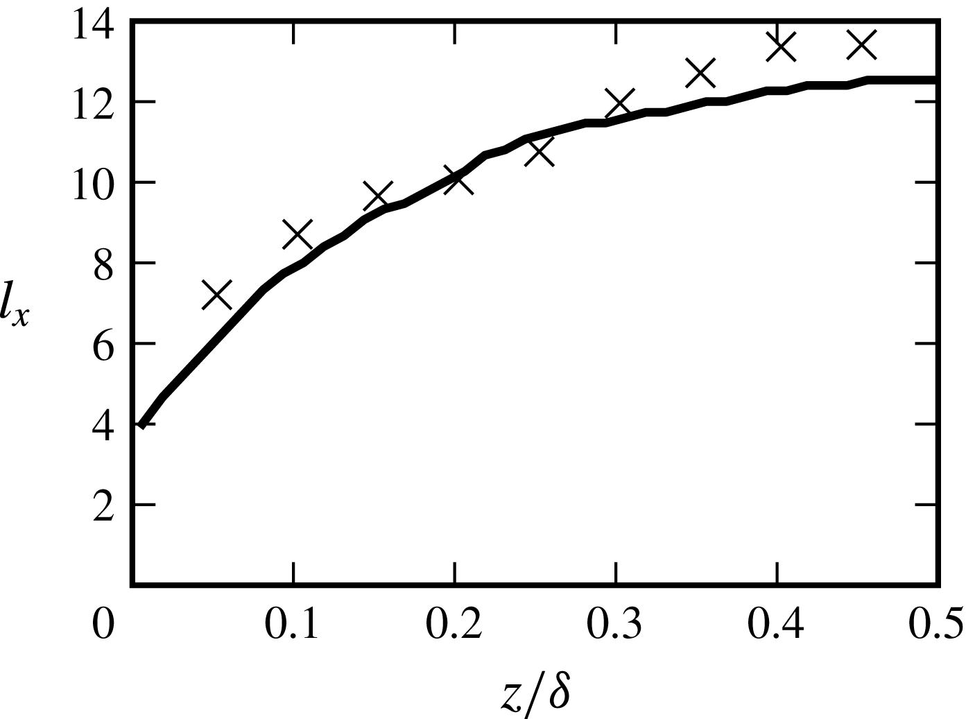
Figure 3 shows the variation of the streamwise length
 $l_{x}$
with height. The lengths in the precursor domain are simply calculated using an inverse Fourier transform by taking advantage of homogeneity in the
 $x$
and
 $y$
directions. The main domain is not homogeneous. Therefore, the correlations are calculated in the physical domain for a downstream point furthest away from the turbine row, i.e.
 ${\mathcal{R}}_{xx}(\unicode[STIX]{x0394}x,x=5.95\unicode[STIX]{x1D6FF},y=2\unicode[STIX]{x1D6FF},z)$
. The same streamwise location is also employed in the analysis of the further sections. We only make use of the upstream data to calculate
 $l_{x}$
in the main domain – downstream data are contaminated by the fringe region.
We see in figure 3 that
 $l_{x}$
in the precursor domain increases rapidly for
 $z/\unicode[STIX]{x1D6FF}<0.25$
, and remains nearly uniform at higher altitudes. The same trend with very similar length scales is also observed in LES simulations of Fang & Porté-Agel (Reference Fang and Porté-Agel2015) for a neutral ABL. It is further observed that length scales calculated at the selected streamwise–spanwise station (
 $\boldsymbol{x}_{p}=(5.95\unicode[STIX]{x1D6FF},2\unicode[STIX]{x1D6FF},z)$
) in the main domain are subject to some statistical scatter. We remark that these values are calculated with respect to single reference point, hence subject to uncertainties due to limited sampling that is especially influential for the long range. Furthermore, as VLSMs are largest scales of the flow, there might be some minor lateral influence of the turbine row standing at
 $y=0$
on VLSMs passing through the selected station
 $2\unicode[STIX]{x1D6FF}$
. Despite these limitations, we see main domain length scales follow roughly the ones in the precursor domain with similar trends. Therefore, we will assume that streamwise statistics of VLSMs that are read into the main domain are only marginally influenced by the grid transition.
Evolution of spanwise spectral densities in the transition region of the main domain at
 $z=0.1\unicode[STIX]{x1D6FF},0.25\unicode[STIX]{x1D6FF}$
.
 $\unicode[STIX]{x1D706}_{y}=2\unicode[STIX]{x03C0}/k_{y}$
is the spanwise wavelength. (a,c) Premultiplied spectrum
 $k_{y}E_{xx}$
; (b,d) premultiplied cospectrum
 $k_{y}E_{xz}$
. The dashed lines at
 $\unicode[STIX]{x1D706}_{y}/\unicode[STIX]{x1D6FF}=0.0533$
demonstrate the cutoff wavelength of the precursor domain.

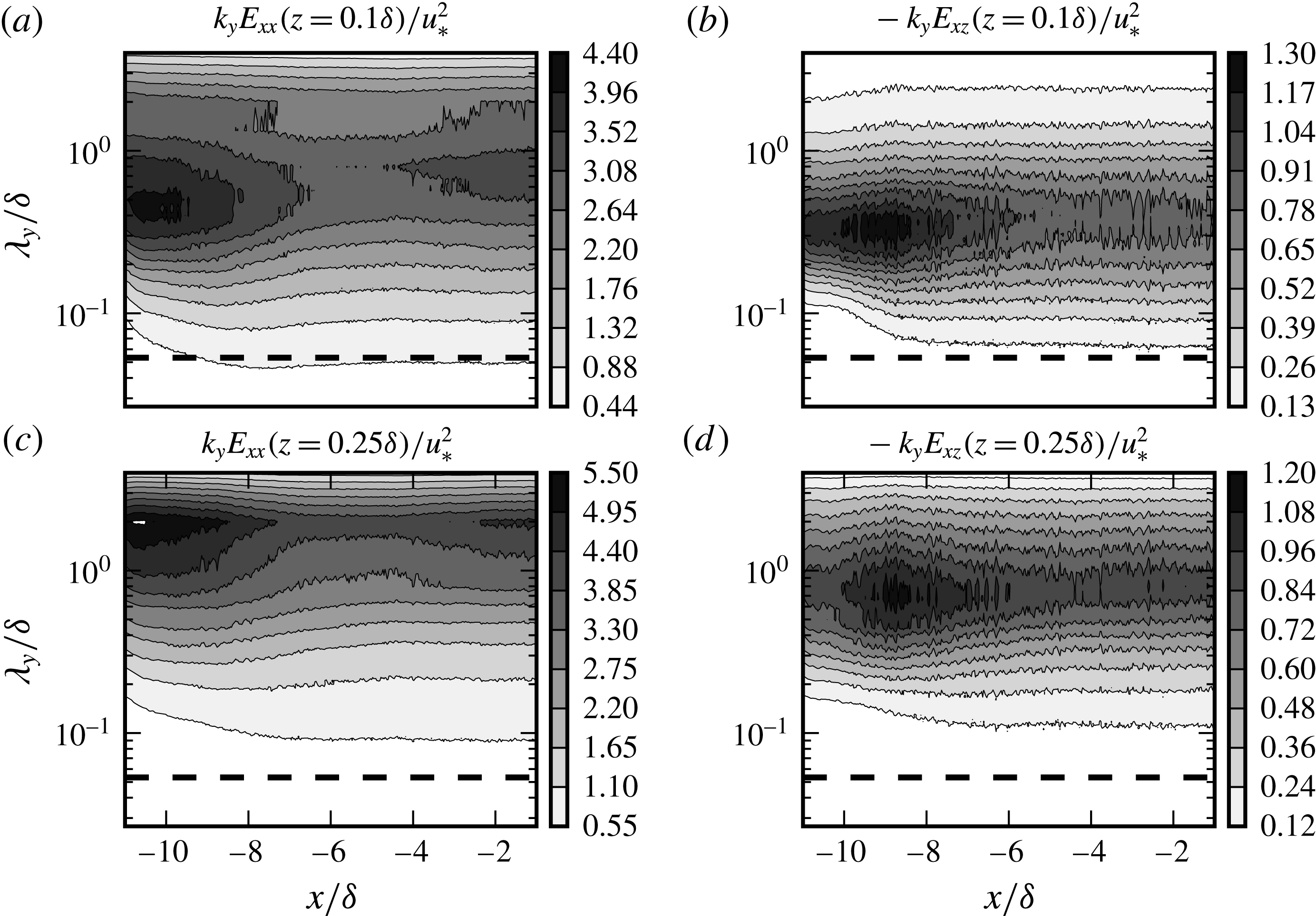
We now turn to the effects of the grid transition on spectral densities. Figure 4 demonstrates the spanwise premultiplied spectra of streamwise fluctuations
 $k_{y}E_{xx}=k_{y}\langle \widehat{u}_{x}^{\prime }(k_{y},x,z,t)\widehat{u}_{x}^{\prime \ast }(k_{y},x,z,t)\rangle$
, and the spanwise premultiplied cospectra
 $k_{y}E_{xz}=-k_{y}\langle \widehat{u}_{x}^{\prime }(k_{y},x,z,t)\widehat{u}_{z}^{\prime \ast }(k_{y},x,z,t)\rangle$
in the transition region at
 $z=0.1\unicode[STIX]{x1D6FF},0.25\unicode[STIX]{x1D6FF}$
. The dashed lines in these figures indicate the cutoff wavelength of the precursor domain. Both the spectra and cospectra show strong variations in large scales in parallel to the evolution of the moments in figure 2. For cospectra, the transfer among scales is relatively faster, and the density contours smooth out around
 $x/\unicode[STIX]{x1D6FF}\approx 5$
, and remain constant in the remaining part of the transition region, cf. figure 4(b,d). Moreover, the spectral peaks remain approximately at the same wavelength with the precursor domain, i.e.
 $\unicode[STIX]{x1D706}_{y}^{max}\approx 0.3\unicode[STIX]{x1D6FF}$
for
 $z=0.1\unicode[STIX]{x1D6FF}$
, and
 $\unicode[STIX]{x1D706}_{y}^{max}\approx 0.8\unicode[STIX]{x1D6FF}$
for
 $z=0.25\unicode[STIX]{x1D6FF}$
. The linear scaling of these peaks with
 $z$
suggests that the dominant Reynolds stress structures in the surface layer are the ones scaling with their height from the ground as in the inertial layer of canonical wall-bounded flows (Jiménez Reference Jiménez2013). The variations in the spectra of streamwise-velocity fluctuations are more pronounced than the cospectra, cf. figure 4(a,c). Similar to the cospectra, the spectra have strong transitions in the entrance region until approximately
 $x/\unicode[STIX]{x1D6FF}\approx -6$
. Subsequently, a relatively smooth region with approximately horizontal contours follow at both heights until
 $x/\unicode[STIX]{x1D6FF}\approx -4$
. Following this streamwise point, a rise in the energy content is observed in long wavelengths, and eventually the spectra settle at around
 $x/\unicode[STIX]{x1D6FF}\approx -2$
.
Besides the variations in large scales, figure 4 also indicates a cascade towards smaller scales on the finer grid of main domain. At
 $z/\unicode[STIX]{x1D6FF}=0.1$
, this cascade is relatively fast, and an equilibrium is reached at around
 $x/\unicode[STIX]{x1D6FF}\approx -8$
, cf. the contour lines in short-wavelength range (
 $\unicode[STIX]{x1D706}_{x}<0.1\unicode[STIX]{x1D6FF}$
) in figure 4(a,b). The cascade occurs more slowly at the higher altitude
 $z/\unicode[STIX]{x1D6FF}=0.25$
, where a state of equilibrium is reached at around
 $x/\unicode[STIX]{x1D6FF}\approx -5$
, cf. figure 4(c,d).
3 The average turbulent transport
This section is devoted to basic analysis of Reynolds-averaged statistics around the turbine row. In wind-energy applications, the recovery rate of wake momentum deficit plays a key role for power extraction. Therefore, our focus is mainly on the turbulent transport of streamwise momentum, which is a main contributor to the wake recovery process.
3.1 The Reynolds shear stress for the cross-stream transport
Before we start our analysis of Reynolds-averaged fields, we introduce a new Reynolds shear stress definition to utilize the presentation of cross-stream turbulent transport of streamwise momentum. Unlike in the homogeneous ABL, the cross-stream transport around a turbine row has an additional component in the spanwise direction, i.e.
 $\langle \widetilde{u}_{x}^{\prime }\widetilde{u}_{y}^{\prime }\rangle$
. Instead of presenting the two Reynolds shear stresses
 $\langle \widetilde{u}_{x}^{\prime }\widetilde{u}_{y}^{\prime }\rangle$
and
 $\langle \widetilde{u}_{x}^{\prime }\widetilde{u}_{z}^{\prime }\rangle$
separately, we will unify them into one component by applying a simple vectorial transformation to the total turbulent flux.
Intrinsic coordinates of the flux lines, which are the tangent lines to
 $\unicode[STIX]{x1D731}=\langle \widetilde{u}_{x}^{\prime }\widetilde{u}_{y}^{\prime }\rangle \hat{\boldsymbol{e}}_{y}+\langle \widetilde{u}_{x}^{\prime }\widetilde{u}_{z}^{\prime }\rangle \hat{\boldsymbol{e}}_{z}=\langle \widetilde{u}_{x}^{\prime }\widetilde{u}_{\unicode[STIX]{x1D709}}^{\prime }\rangle \hat{\boldsymbol{e}}_{\unicode[STIX]{x1D709}}$
.

The turbulent flux of streamwise momentum through a curve
 $C$
in transverse
 $y{-}z$
plane is defined as follows
 $$\begin{eqnarray}\langle M_{x}\rangle =\int _{C}\unicode[STIX]{x1D731}\boldsymbol{\cdot }\hat{\boldsymbol{n}}\,\text{d}s,\end{eqnarray}$$
where
 $\hat{\boldsymbol{n}}$
is the curve normal, and
 $\unicode[STIX]{x1D731}$
is the turbulent flux vector for streamwise momentum, which contains the tangential Reynolds stresses
 $$\begin{eqnarray}\unicode[STIX]{x1D731}=\langle \widetilde{u}_{x}^{\prime }\widetilde{u}_{y}^{\prime }\rangle \hat{\boldsymbol{e}}_{y}+\langle \widetilde{u}_{x}^{\prime }\widetilde{u}_{z}^{\prime }\rangle \hat{\boldsymbol{e}}_{z}.\end{eqnarray}$$
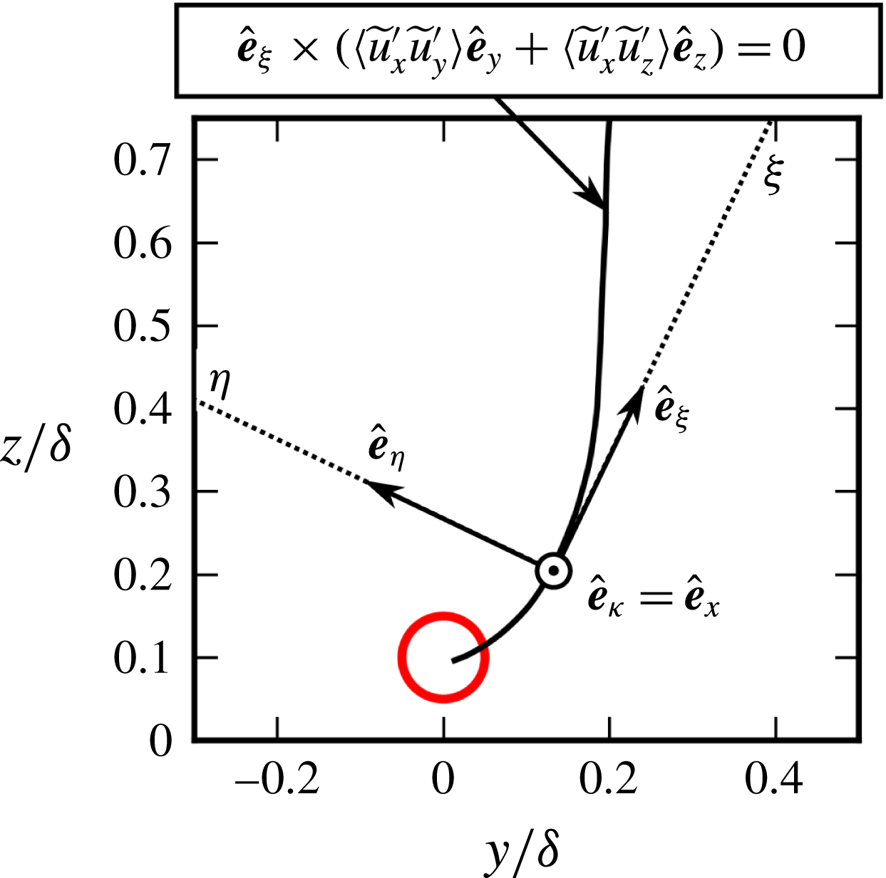
This turbulent flux vector can be utilized to analyse the total in-plane turbulent transport. To this end, we first introduce the concept of flux lines as the family of curves everywhere tangent to
 $\unicode[STIX]{x1D731}$
, cf. figure 5. At each point on the flux line we then introduce an orthonormal set of unit vectors that are in the tangential
 $\hat{\boldsymbol{e}}_{\unicode[STIX]{x1D709}}=-\unicode[STIX]{x1D731}/\Vert \unicode[STIX]{x1D731}\Vert$
, bi-normal
 $\hat{\boldsymbol{e}}_{\unicode[STIX]{x1D705}}=\hat{\boldsymbol{e}}_{x}$
and normal
 $\hat{\boldsymbol{e}}_{\unicode[STIX]{x1D702}}=\hat{\boldsymbol{e}}_{\unicode[STIX]{x1D705}}\times \hat{\boldsymbol{e}}_{\unicode[STIX]{x1D709}}$
directions with respect to the flux line. In these local coordinates, the tangential Reynolds flux vector has no component in the normal direction, i.e.
 $\langle \widetilde{u}_{\unicode[STIX]{x1D705}}^{\prime }\widetilde{u}_{\unicode[STIX]{x1D702}}^{\prime }\rangle =0$
, and therefore, simplifies to the following form
 $$\begin{eqnarray}\unicode[STIX]{x1D731}=\langle \widetilde{u}_{\unicode[STIX]{x1D705}}^{\prime }\widetilde{u}_{\unicode[STIX]{x1D709}}^{\prime }\rangle \hat{\boldsymbol{e}}_{\unicode[STIX]{x1D709}}=\langle \widetilde{u}_{x}^{\prime }\widetilde{u}_{\unicode[STIX]{x1D709}}^{\prime }\rangle \hat{\boldsymbol{e}}_{\unicode[STIX]{x1D709}},\end{eqnarray}$$
where
 $\widetilde{u}_{\unicode[STIX]{x1D709}}^{\prime }=\widetilde{\boldsymbol{u}}^{\prime }\boldsymbol{\cdot }\hat{\boldsymbol{e}}_{\unicode[STIX]{x1D709}}$
. In this new formulation the magnitude of the flux vector is simply given by
 $\Vert \unicode[STIX]{x1D731}\Vert =|\langle \widetilde{u}_{x}^{\prime }\widetilde{u}_{\unicode[STIX]{x1D709}}^{\prime }\rangle |$
. The Reynolds shear stress
 $\langle \widetilde{u}_{x}^{\prime }\widetilde{u}_{\unicode[STIX]{x1D709}}^{\prime }\rangle$
together with the flux lines provide a complete description for the in-plane turbulent transport of streamwise momentum, which can be presented in a single contour plot, cf. e.g. figure 7(b,d) in the following section.
3.2 Reynolds-averaged fields
The resolved mean streamwise velocity and tangential Reynolds stresses at hub height and symmetry half-plane. Short lines represent the turbines. The lines at
 $x=1.05\unicode[STIX]{x1D6FF}=1.5S_{x}$
and
 $x=5.95\unicode[STIX]{x1D6FF}=8.5S_{x}$
show the location of transverse planes in figure 7.

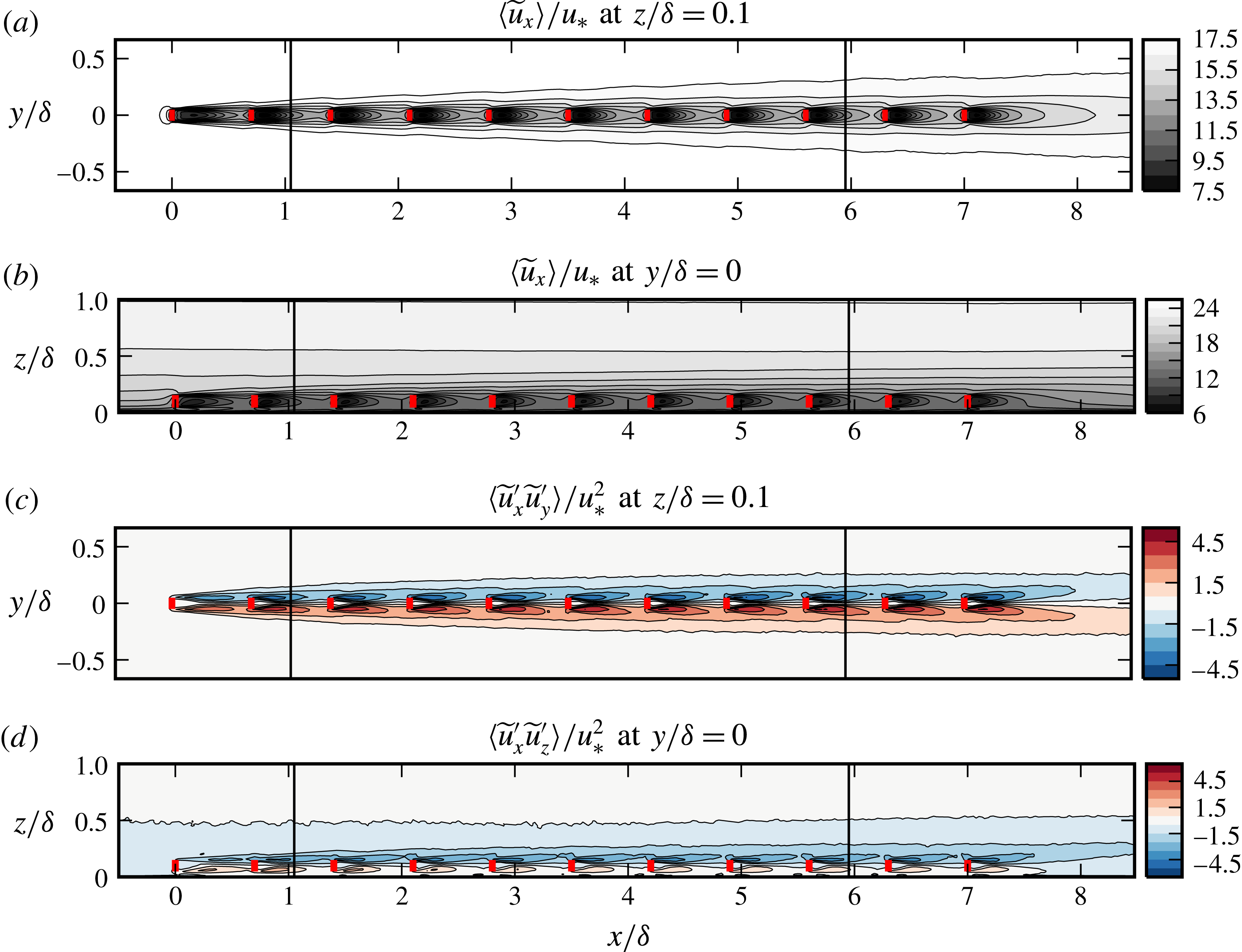
Figure 6 demonstrates the time-averaged resolved streamwise velocity
 $\langle \widetilde{u}_{x}\rangle$
and tangential Reynolds stresses
 $\langle \widetilde{u}_{x}^{\prime }\widetilde{u}_{y}^{\prime }\rangle$
and
 $\langle \widetilde{u}_{x}^{\prime }\widetilde{u}_{z}^{\prime }\rangle$
on the horizontal plane
 $z/\unicode[STIX]{x1D6FF}=0.1$
at hub height and on the symmetry half-plane
 $y/\unicode[STIX]{x1D6FF}=0$
. In these figures, darker colours are employed to present the values in the turbine wakes. In this regard, darker shadings indicate low values of streamwise velocity, and high values of Reynolds stress. In figure 6(a), the outer most contour lines mark the growth of an internal layer due to momentum deficit caused by the drag of the turbines. Inside this internal layer, the evolution of turbine wakes can be seen for approximately
 $-D<y<D$
. We denote this region with intense momentum deficit as the wake region. We see here that the wakes of downstream turbines recover faster, hence they are shorter. The wakes of the ninth turbine at
 $x=5.6\unicode[STIX]{x1D6FF}$
and tenth turbine at
 $x=6.3\unicode[STIX]{x1D6FF}$
have only marginal differences suggesting a well-developed transport towards the central wake region. In the side view in figure 6(b), the contour line at
 $z\approx 0.55\unicode[STIX]{x1D6FF}$
is almost horizontal. Therefore, the effect of the turbine row on the outermost ABL structures appears to be limited. Nevertheless, we see that the internal layer still reaches high altitudes, cf. the inclined contour line starting at
 $z\approx 0.3\unicode[STIX]{x1D6FF}$
close to
 $x=-\unicode[STIX]{x1D6FF}$
and ending at
 $z\approx 0.4\unicode[STIX]{x1D6FF}$
close to
 $x=9\unicode[STIX]{x1D6FF}$
. We observe again nearly identical patterns in side view for
 $z<0.2\unicode[STIX]{x1D6FF}=2D$
in the wake of downstream turbines. Therefore, we define the vertical dimension of the wake region as
 $z<0.2\unicode[STIX]{x1D6FF}=2D$
.
The effect of a growing internal layer can also be seen in Reynolds stresses in figure 6(c,d). The wake region in these panels is characterized by high Reynolds stresses due to dynamic wake motions. In most downstream positions, we see periodic wake patterns with a streamwise wavelength of
 $S_{x}$
, which suggests a fast development also for second-order quantities in the wake region.
Mean fields at
 $x=1.05\unicode[STIX]{x1D6FF}=1.5S_{x}$
and
 $x=5.95\unicode[STIX]{x1D6FF}=8.5S_{x}$
. Contours of (a,c) the mean streamwise velocity
 $\langle \widetilde{u}_{x}\rangle$
; (b,d) the shear stress modulus
 $|\langle \widetilde{u}_{x}^{\prime }\widetilde{u}_{\unicode[STIX]{x1D709}}^{\prime }\rangle |$
, cf. (3.3). Arrowed curves in both panels represent the flux lines that are everywhere tangent to
 $\unicode[STIX]{x1D731}=\langle \widetilde{u}_{x}^{\prime }\widetilde{u}_{y}^{\prime }\rangle \hat{\boldsymbol{e}}_{y}+\langle \widetilde{u}_{x}^{\prime }\widetilde{u}_{z}^{\prime }\rangle \hat{\boldsymbol{e}}_{z}=\langle \widetilde{u}_{x}^{\prime }\widetilde{u}_{\unicode[STIX]{x1D709}}^{\prime }\rangle \hat{\boldsymbol{e}}_{\unicode[STIX]{x1D709}}$
. The circles demonstrate the projected location of turbines onto the planes.

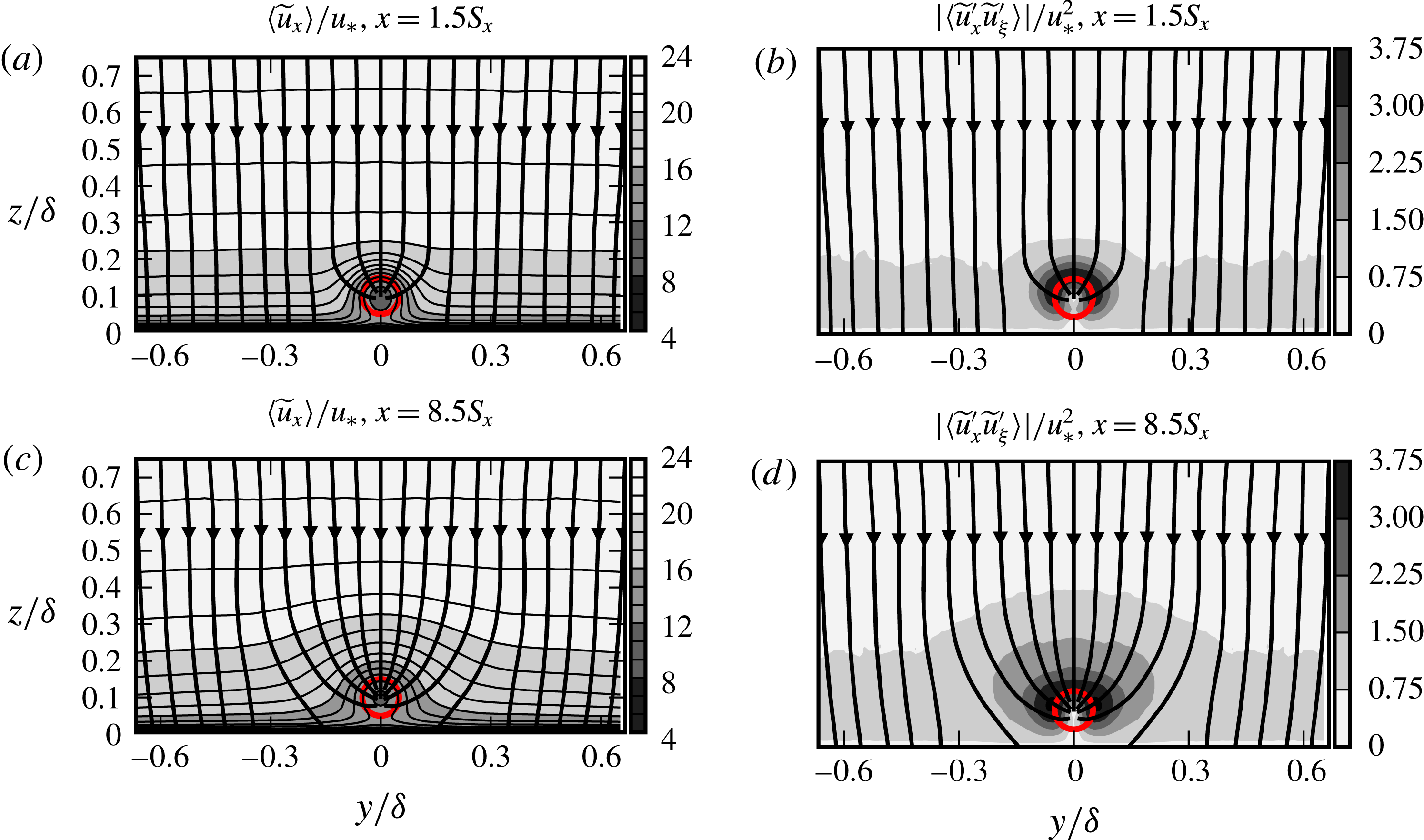
Now we will analyse the turbulent transport towards the wakes using the Reynolds shear stress
 $\langle \widetilde{u}_{x}^{\prime }\widetilde{u}_{\unicode[STIX]{x1D709}}^{\prime }\rangle$
and the flux lines (cf. figure 5). Two vertical planes are selected for further presentation of the average flow around the turbines. To this end, the plane at
 $x=1.05\unicode[STIX]{x1D6FF}=1.5S_{x}$
represents an initial state, and the plane
 $x=5.95\unicode[STIX]{x1D6FF}=8.5S_{x}$
represents a more developed state along the turbine row. Figure 7(a,c) shows the isolines of the mean streamwise velocity
 $\langle \widetilde{u}_{x}\rangle$
and the flux lines. In figure 7(c) at
 $x=8.5S_{x}$
, we see the lateral spreading of the internal layer with lower momentum roughly up to
 $-5D<y<5D$
around the turbine row. Such a wide spreading is not observed at the upstream plane at
 $x=1.5S_{x}$
in figure 7(a). Furthermore, we see on both planes that isolines of
 $\langle \widetilde{u}_{x}\rangle$
and the flux lines are nearly orthogonal outside the wake region, suggesting a local shear-dominated production for turbulence. Moreover, the turbine wakes act as a momentum sink, and near the turbines the turbulent flux is towards the wake, not towards the wall.
We have plotted the contours of
 $|\langle \widetilde{u}_{x}^{\prime }\widetilde{u}_{\unicode[STIX]{x1D709}}^{\prime }\rangle |$
on two selected vertical planes in figure 7(b,d). For the downstream plane, the contour levels have the tendency to spread laterally suggesting a more effective turbulent momentum transport from the sideways direction. This is also observed by Meyers & Meneveau (Reference Meyers and Meneveau2013) in wind farms with large spanwise spacings between the rows by visualizing the momentum transport tubes.
In summary, the considered flow can be decomposed into three regions: the unperturbed ABL region far from the turbine row; a wake region that quickly reaches an equilibrium state and develops periodic wake patterns with a streamwise spacing of
 $S_{x}$
; and a continuously growing internal layer around the central wake region. In an asymptotic state where the row extends to infinity in the streamwise direction, the internal layer is expected to grow until occupying the entire ABL thickness.
4 Statistics of the filtered fields
In this section, we investigate the interaction of VLSMs and turbine row using a spatial scale decomposition. To this end, we extract long streamwise-wavelength motions using a spectral cutoff filter. The details of the filter are presented in § 4.1, and Reynolds-averaged filtered fields are discussed in § 4.2.
4.1 Spatial scale decomposition
The spatial scale decomposition of fluctuating velocity fields or signals into large-scale and small-scale components has been previously employed by various researchers to investigate the multiscale characteristics of boundary layers. In a high Reynolds number turbulent boundary layer, Mathis et al. (Reference Mathis, Hutchins and Marusic2009) applied a spectral cutoff to separate near-wall time histories into large-scale (
 $\unicode[STIX]{x1D706}_{x}/\unicode[STIX]{x1D6FF}>1$
) and small-scale components (
 $\unicode[STIX]{x1D706}_{x}/\unicode[STIX]{x1D6FF}<1$
). They associated the large-scale components with VLSMs penetrating to the near wall, and analysed their nonlinear interactions with smaller-scale components. Chung & McKeon (Reference Chung and McKeon2010) employed a sliding window top-hat filter to fluctuating velocity fields in a long channel LES database, and analysed large-scale–small-scale interactions across the channel.
The cutoff length scales are usually determined from premultiplied energy spectra maps. While Mathis et al. (Reference Mathis, Hutchins and Marusic2009) have found the cutoff at the streamwise wavenumber
 $\unicode[STIX]{x1D706}_{x}/\unicode[STIX]{x1D6FF}=1$
to be sufficient to isolate VLSMs in the near-wall layer, Guala et al. (Reference Guala, Hommema and Adrian2006) considered VLSMs to be the motions with
 $\unicode[STIX]{x1D706}_{x}/\unicode[STIX]{x1D6FF}>\unicode[STIX]{x03C0}$
in the outer layer of a pipe flow. The selection of this longer wavelength threshold was required to distinguish VLSMs from LSMs that reach a maximum length of approximately
 $\unicode[STIX]{x1D706}_{x}/\unicode[STIX]{x1D6FF}=3$
at
 $z/\unicode[STIX]{x1D6FF}=0.5$
. Both type of motions were characterized with distinctive peaks in the bimodal premultiplied spectra. In another pipe flow experiment, Bailey & Smits (Reference Bailey and Smits2010) found LSMs occurring at longer wavelengths, hence classified the motions in the range
 $\unicode[STIX]{x1D706}_{x}/\unicode[STIX]{x1D6FF}>2\unicode[STIX]{x03C0}$
as VLSMs.
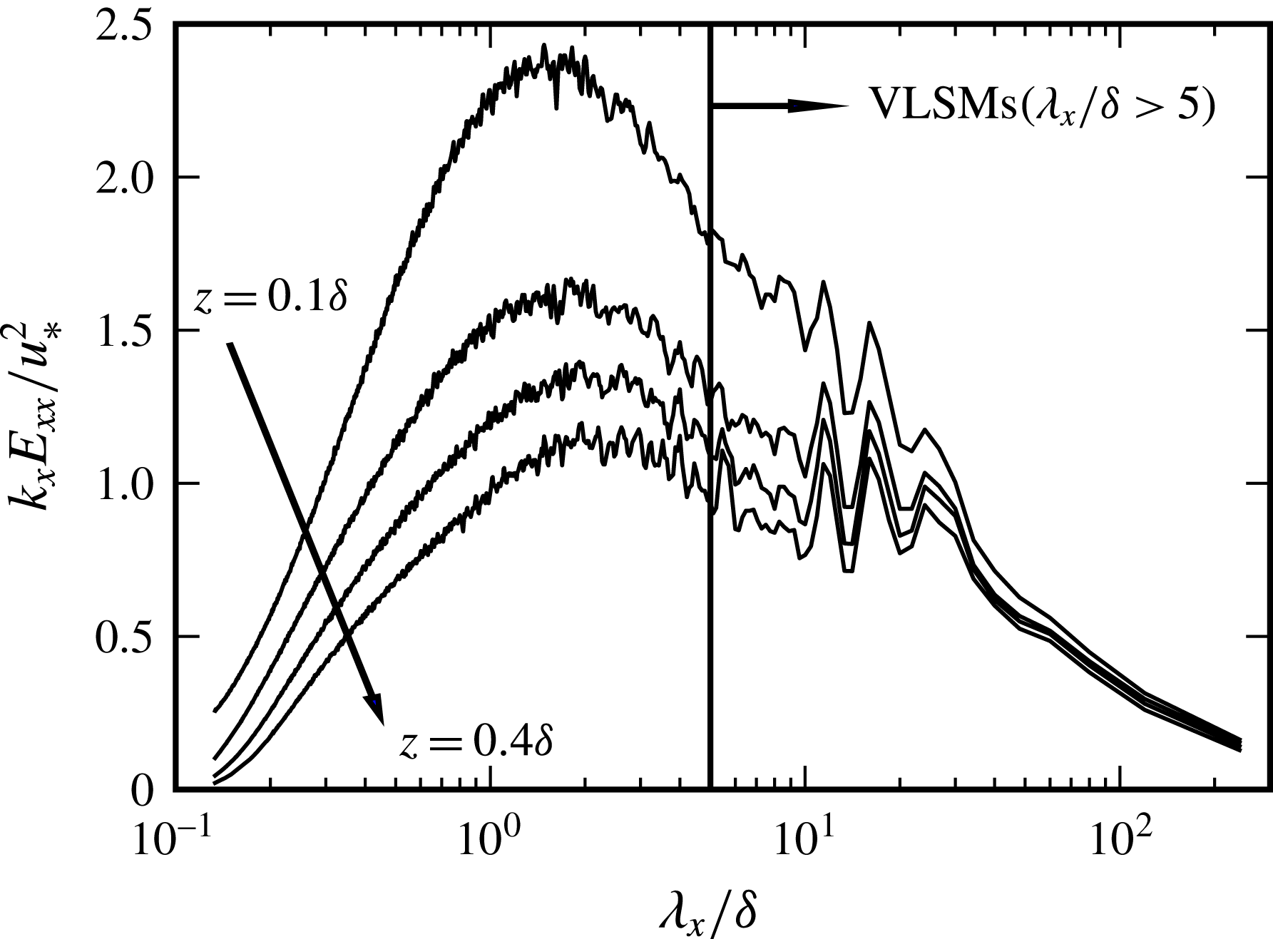
Premultiplied spectra of streamwise-velocity fluctuations as functions of non-dimensional streamwise wavelength at
 $z=0.1\unicode[STIX]{x1D6FF},\ldots ,0.4\unicode[STIX]{x1D6FF}$
in the precursor domain.

Figure 8 shows the streamwise premultiplied spectra
 $k_{x}E_{xx}(\unicode[STIX]{x1D706}_{x})$
at four different heights
 $z=0.1\unicode[STIX]{x1D6FF},\ldots ,0.4\unicode[STIX]{x1D6FF}$
in the precursor domain. Each spectrum shows a bimodal distribution with two peaks corresponding to LSMs and VLSMs. The LSMs peak at shorter wavelengths moves from
 $\unicode[STIX]{x1D706}_{x}/\unicode[STIX]{x1D6FF}=0.5$
to approximately
 $\unicode[STIX]{x1D706}_{x}/\unicode[STIX]{x1D6FF}=3$
with increasing height. The data at longer wavelengths are noise dominated, hence we estimate the peak corresponding to VLSMs to at approximately
 $\unicode[STIX]{x1D706}_{x}/\unicode[STIX]{x1D6FF}\approx 15{-}20$
with less height dependence than with the LSMs. Furthermore, we see that after approximately
 $\unicode[STIX]{x1D706}_{x}/\unicode[STIX]{x1D6FF}>5$
the slope of the spectra appear to flatten due to increasing contributions from VLSMs. Therefore, we assume that VLSMs are dominant energetic elements for the range
 $\unicode[STIX]{x1D706}_{x}/\unicode[STIX]{x1D6FF}>5$
, and select
 $\unicode[STIX]{x1D706}_{x}^{c}/\unicode[STIX]{x1D6FF}=5$
as the cutoff wavelength. The selected cutoff wavelength corresponds to
 $\unicode[STIX]{x1D706}_{x}^{c}/D=50$
in terms of turbine diameter.
The sharp spectral cutoff at a streamwise wavelength
 $\unicode[STIX]{x1D706}_{x}^{c}$
is defined in the Fourier space as follows
 $$\begin{eqnarray}\text{G}(\unicode[STIX]{x1D706}_{x};\unicode[STIX]{x1D706}_{x}^{c})=\left\{\begin{array}{@{}l@{}}1,\quad \text{if }|\unicode[STIX]{x1D706}_{x}|\geqslant \unicode[STIX]{x1D706}_{x}^{c},\\ 0,\quad \text{if }|\unicode[STIX]{x1D706}_{x}|<\unicode[STIX]{x1D706}_{x}^{c}.\end{array}\right.\end{eqnarray}$$
This filter is employed to decompose the fluctuating fields into two components
 $$\begin{eqnarray}\widetilde{\boldsymbol{u}}^{\prime }=\widetilde{\boldsymbol{u}}^{L}+\widetilde{\boldsymbol{u}}^{S},\end{eqnarray}$$
where
 $\widetilde{\boldsymbol{u}}^{L}=\text{G}(\unicode[STIX]{x1D706}_{x};5\unicode[STIX]{x1D6FF})\circ \widetilde{\boldsymbol{u}}^{\prime }$
contains the very-large-scale components of the flow, and
 $\widetilde{\boldsymbol{u}}^{S}$
contains the residual smaller-scale motions. We note that
 $\langle \widetilde{u}_{i}^{L}\widetilde{u}_{j}^{S}\rangle =0$
, hence Reynolds stresses can also be decomposed into two components
 $$\begin{eqnarray}\langle \widetilde{u}_{i}^{\prime }\widetilde{u}_{j}^{\prime }\rangle =\langle \widetilde{u}_{i}^{L}\widetilde{u}_{j}^{L}\rangle +\langle \widetilde{u}_{i}^{S}\widetilde{u}_{j}^{S}\rangle ,\end{eqnarray}$$
where
 $\langle \widetilde{u}_{i}^{L}\widetilde{u}_{j}^{L}\rangle$
is the large-scale Reynolds stress, and
 $\langle \widetilde{u}_{i}^{S}\widetilde{u}_{j}^{S}\rangle$
is the small-scale Reynolds stress. These scale-decomposed Reynolds stresses will be investigated in the next section.
4.2 Scale-decomposed Reynolds stresses
In § 3, we observed a significantly growing internal layer in the streamwise direction around the turbine row. This internal layer is characterized by a momentum deficit and high turbulence content. It reaches lateral dimensions that are an order of magnitude larger than the turbines, and spreads up to
 $0.5\unicode[STIX]{x1D6FF}$
in higher atmosphere. These dimensions suggest that there may be significant modifications to large-scale elements in ABL while they move downstream around the row. In this section, we characterize these modifications using the two-scale decomposition of Reynolds stresses, cf. (4.3). Moreover, we quantify the contribution of these very-large-scale elements to turbulent energy and momentum transport in the wake region.
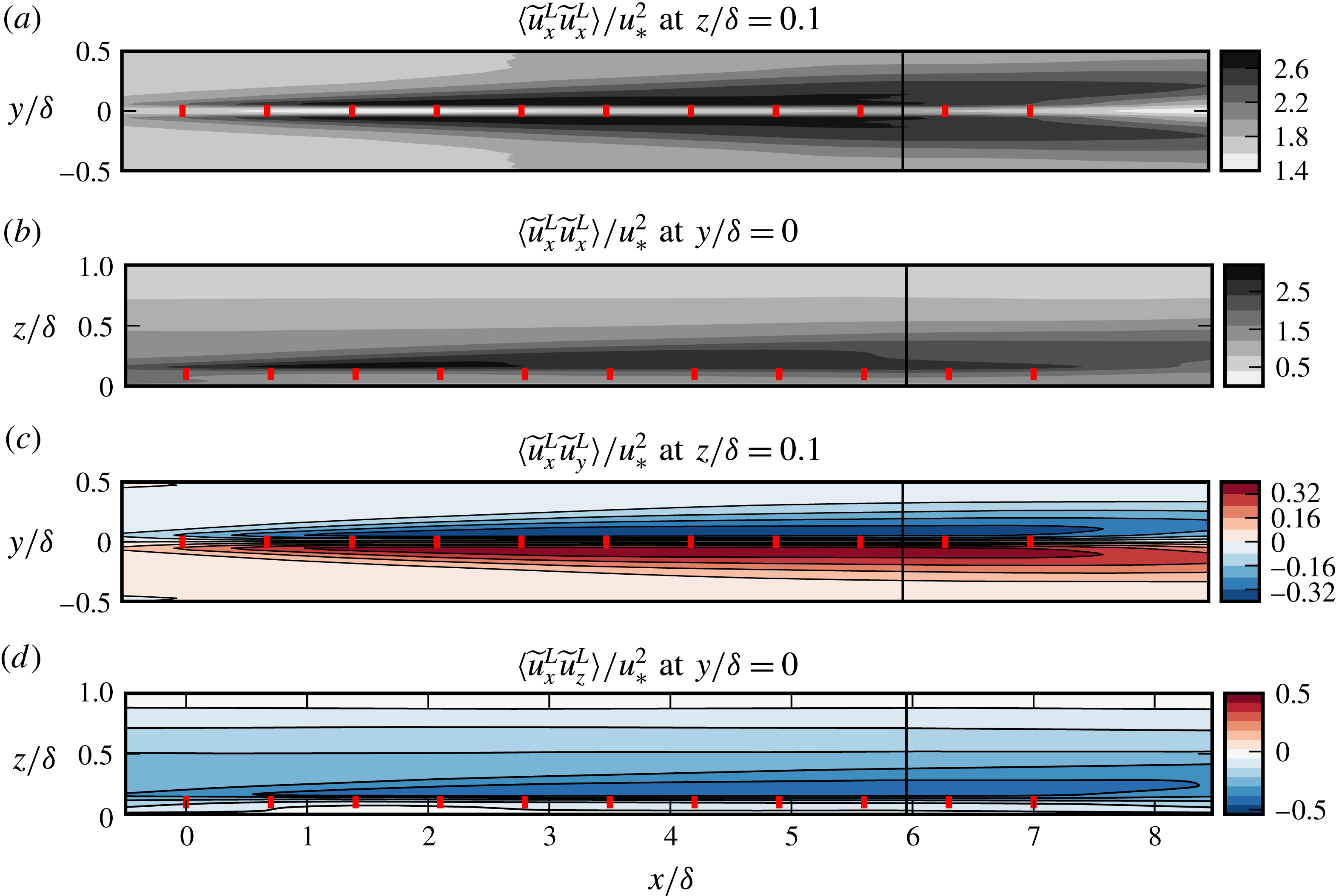
Figure 9 demonstrates the large-scale components of streamwise turbulent kinetic energy,
 $\langle \widetilde{u}_{x}^{L}\widetilde{u}_{x}^{L}\rangle$
, and tangential Reynolds stresses,
 $\langle \widetilde{u}_{x}^{L}\widetilde{u}_{y}^{L}\rangle$
and
 $\langle \widetilde{u}_{x}^{L}\widetilde{u}_{z}^{L}\rangle$
, in the horizontal plane
 $z/\unicode[STIX]{x1D6FF}=0.1$
at hub height and in the symmetry half-plane
 $y/\unicode[STIX]{x1D6FF}=0$
. Figure 9(a,b) shows an increase in the energy content of the long-wavelength motions compared to the unperturbed ABL, which suggests strong modifications on VLSMs when they meet the turbine row. As the general trends of the contours are similar to those of the streamwise velocity in figure 6(a,b), the rise in the energy can be attributed to the interaction of VLSMs with the intense mean shear field developing around the row. We note the highest values are reached in the free-shear layers behind the turbines, where the shear peaks.
Large-scale streamwise kinetic energy and tangential Reynolds stresses at hub height and symmetry half-plane. The fields are obtained using a spectral cutoff at
 $\unicode[STIX]{x1D706}_{x}=5\unicode[STIX]{x1D6FF}$
. Short lines represent the turbines. The lines
 $x=5.95\unicode[STIX]{x1D6FF}=8.5S_{x}$
show the location of transverse planes in figure 10.

The magnitude of the large-scale Reynolds stresses also increases around the turbine row in parallel to the large-scale turbulent kinetic energy, cf. figure 9(c,d). The direction of the stresses is reminiscent of wake structures, cf. the wake regions in 6(c,d). In this organization, there is a positive transport of streamwise momentum towards the turbine wakes, i.e. low-speed fluid is moved away from the row, and high-speed fluid is brought in. Therefore, interaction of the VLSMs with the turbine row, and the mean shear field around it, produce very-large-scale structures reminiscent of wake turbulence.
We now turn to the transverse distribution of large-scale and small-scale kinetic energy and Reynolds shear stresses. For analysis of the turbulent transport, we adapt the coordinate transformation introduced in § 3.1 to the scale-decomposed Reynolds stresses. To this end, for each scale we define flux lines as tangent lines to the scale-decomposed flux vector, e.g.
 $\unicode[STIX]{x1D731}^{L}=\langle \widetilde{u}_{x}^{L}\widetilde{u}_{y}^{L}\rangle \hat{\boldsymbol{e}}_{y}+\langle \widetilde{u}_{x}^{L}\widetilde{u}_{z}^{L}\rangle \hat{\boldsymbol{e}}_{z}$
for the large-scale component, and subsequently, the Reynolds shear stresses
 $\langle \widetilde{u}_{x}^{L}\widetilde{u}_{\unicode[STIX]{x1D709}}^{L}\rangle$
and
 $\langle \widetilde{u}_{x}^{S}\widetilde{u}_{\unicode[STIX]{x1D709}}^{S}\rangle$
are derived on the intrinsic tangents of the corresponding flux lines.
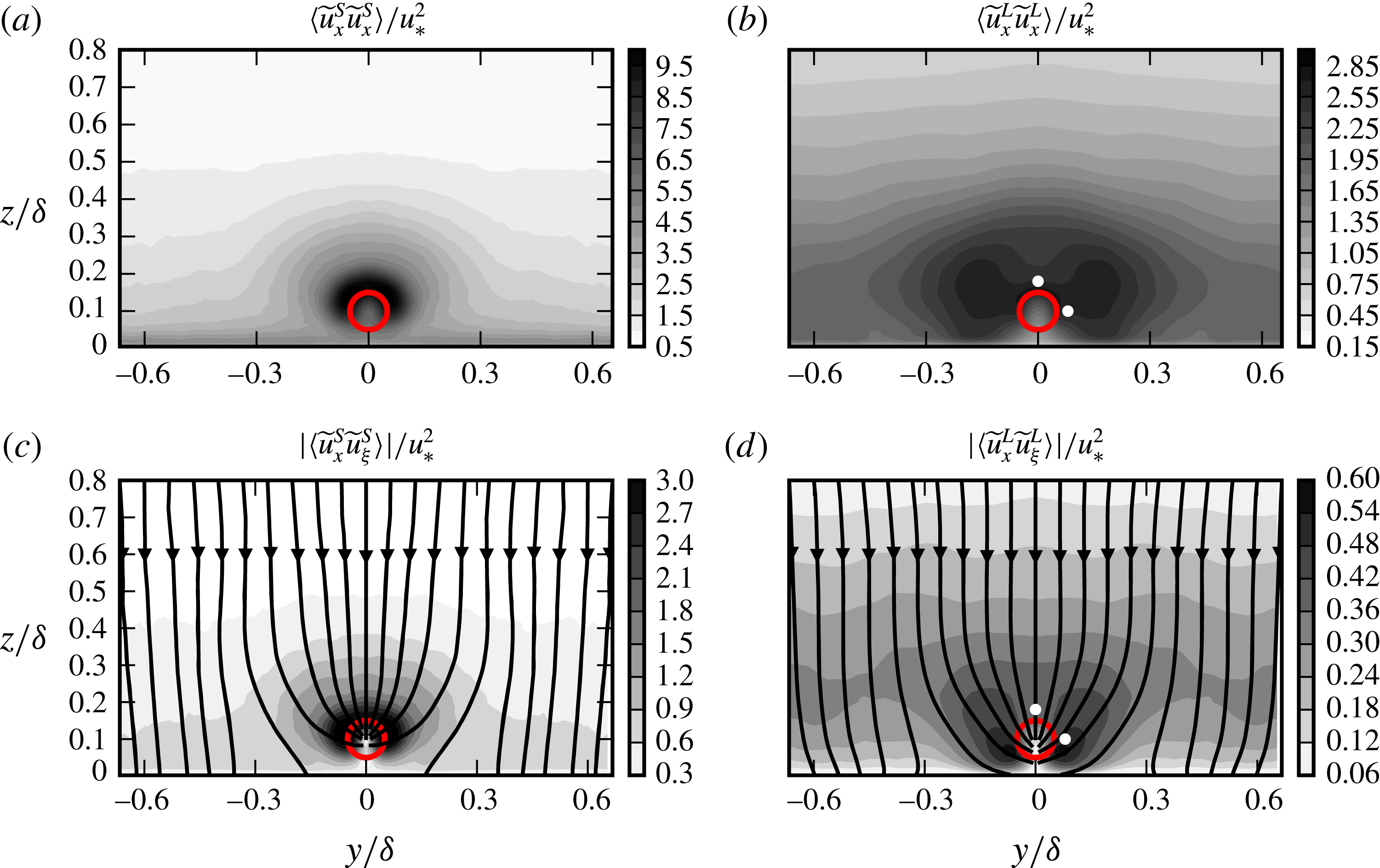
Scale-decomposed turbulent fields using a cutoff at
 $\unicode[STIX]{x1D706}_{x}=5\unicode[STIX]{x1D6FF}$
are shown
 $x=5.95\unicode[STIX]{x1D6FF}=8.5S_{x}$
. (a) Small-scale streamwise energy
 $\langle \widetilde{u}_{x}^{S}\widetilde{u}_{x}^{S}\rangle$
; (b) large-scale streamwise energy
 $\langle \widetilde{u}_{x}^{L}\widetilde{u}_{x}^{L}\rangle$
; (c) small-scale shear stress modulus
 $|\langle \widetilde{u}_{x}^{S}\widetilde{u}_{\unicode[STIX]{x1D709}}^{S}\rangle |=\Vert \unicode[STIX]{x1D731}^{S}\Vert$
, where
 $\unicode[STIX]{x1D731}^{S}=\langle \widetilde{u}_{x}^{S}\widetilde{u}_{y}^{S}\rangle \hat{\boldsymbol{e}}_{y}+\langle \widetilde{u}_{x}^{S}\widetilde{u}_{z}^{S}\rangle \hat{\boldsymbol{e}}_{z}=\langle \widetilde{u}_{x}^{S}\widetilde{u}_{\unicode[STIX]{x1D709}}^{S}\rangle \hat{\boldsymbol{e}}_{\unicode[STIX]{x1D709}}^{S}$
is the small-scale turbulent flux vector. Arrowed lines are the flux lines that are everywhere tangent to
 $\unicode[STIX]{x1D731}^{S}$
; (d) large-scale counterpart of (c). The circles demonstrate the projected location of turbines onto the planes. White markers in (b,d) show the position of the streamwise lines that are used in figure 11.

Figure 10(a,b) shows the streamwise kinetic energy distributions at
 $x=5.95\unicode[STIX]{x1D6FF}=8.5S_{x}$
for small-scale,
 $\langle \widetilde{u}_{x}^{S}\widetilde{u}_{x}^{S}\rangle$
, and large-scale,
 $\langle \widetilde{u}_{x}^{L}\widetilde{u}_{x}^{L}\rangle$
, components respectively. We see in figure 10(a) that
 $\langle \widetilde{u}_{x}^{S}\widetilde{u}_{x}^{S}\rangle$
peaks in the shear layer of the wake region, and decays then in lateral and vertical directions with a similar rate. In contrast, the spatial organization of the very-large-scale energy is more inhomogeneous around the wake region with higher values concentrating in lateral directions, cf. figure 10(b). Similar qualitative behaviours with some differences in detail are also observed in shear stress contours for both small- and large-scale components, cf. figure 10(c,d). Figure 10(c,d) further show that flux lines close to the turbine row are deflected towards the wakes. Therefore, both large-scale and small-scale momentum transport in the vicinity of the row are towards the wake region not towards the ground.
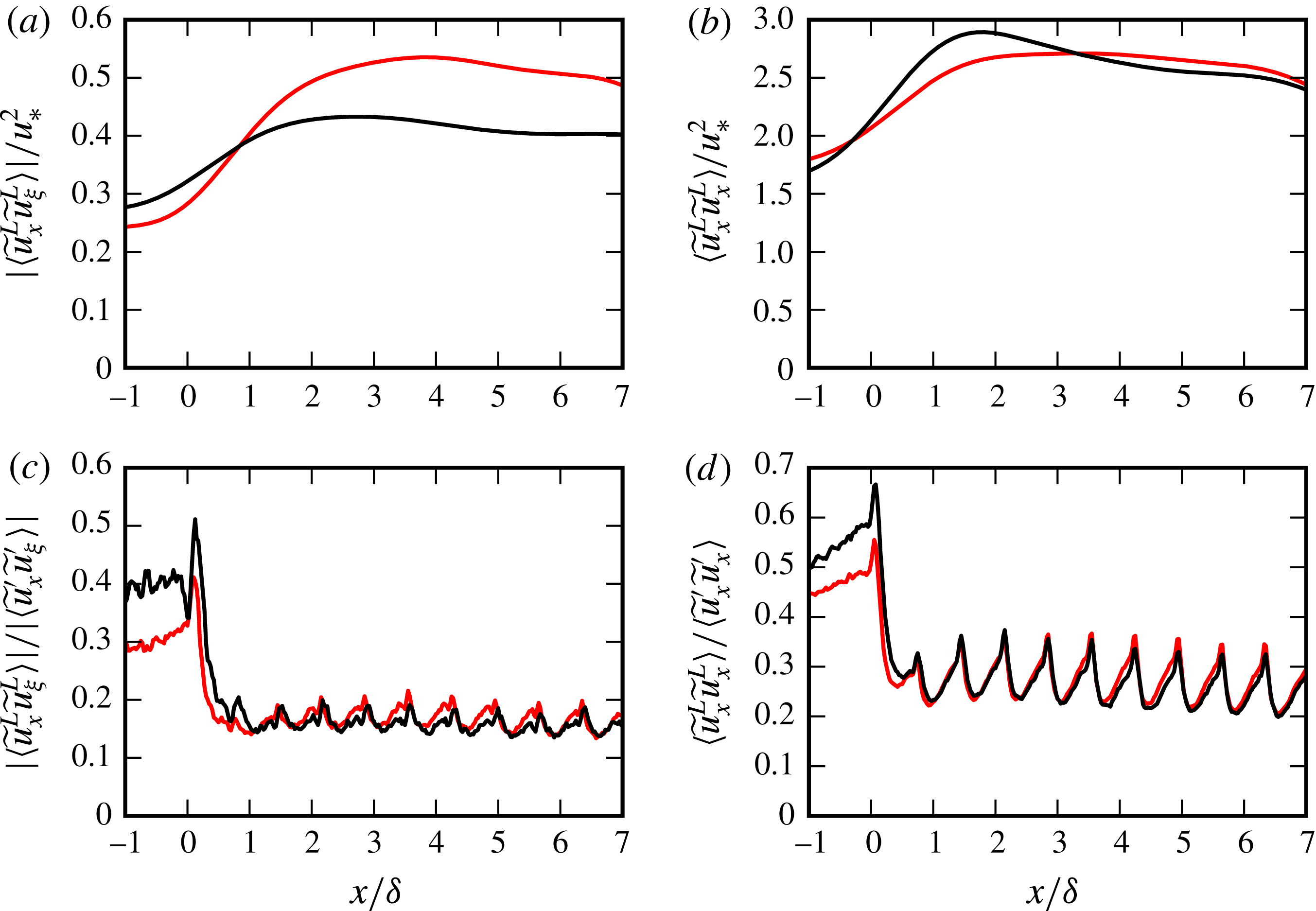
Evolution of the very-large-scale (
 $\unicode[STIX]{x1D706}_{x}>5\unicode[STIX]{x1D6FF}$
) Reynolds shear stress
 $|\langle \widetilde{u}_{x}^{L}\widetilde{u}_{\unicode[STIX]{x1D709}}^{L}\rangle |$
and streamwise kinetic energy
 $\langle \widetilde{u}_{x}^{L}\widetilde{u}_{x}^{L}\rangle$
on two selected lines along the turbines row in the wake shear layer. Light-coloured lines show data along
 $y=0.8D$
,
 $z=D$
, and dark-coloured lines show data along
 $y=0$
,
 $z=1.8D$
, cf. figure 10(b,d) for the position of the lines. (a,b) Absolute values scaled with the friction velocity; (c,d) fractions with respect to the total stress and energy.

So far we have mainly discussed the qualitative properties of the scale-decomposed fields. We now turn to their quantitative properties, e.g. their relative values with respect to the baseline values in the unperturbed ABL, and their overall fraction in the total energy and shear stress. To this end, we focus on the wake region, as the very-large-scale contributions here have direct effect on the turbine power and loading characteristics. Figure 11(a,b) shows the evolution of
 $|\langle \widetilde{u}_{x}^{L}\widetilde{u}_{\unicode[STIX]{x1D709}}^{L}\rangle |$
and
 $\langle \widetilde{u}_{x}^{L}\widetilde{u}_{x}^{L}\rangle$
on two selected streamwise lines in the shear layer of turbines: a sideway line at
 $y=0.8D$
and at the hub-height
 $z=D$
, and a second line above the turbine at
 $z=1.8D$
aligned with the row (
 $y=0$
), cf. white markers in figure 10(b,d). The values at
 $x=-\unicode[STIX]{x1D6FF}$
in figure 11 represent the reference ABL values. It is observed in figure 11(a) that the large-scale Reynolds shear stress increases by approximately
 $100\,\%$
on the lateral line, and reaches a quasi-equilibrium at around
 $x=3\unicode[STIX]{x1D6FF}$
. The increment is milder in the top line where we see
 $50\,\%$
increase. Similar increments with respect to unperturbed ABL values are also observed for large-scale kinetic energy, cf. figure 11(b). In this case, the rise is approximately
 $70\,\%$
on both lines.
Figure 11(c,d) shows the fractions
 $|\langle \widetilde{u}_{x}^{L}\widetilde{u}_{\unicode[STIX]{x1D709}}^{L}\rangle |/|\langle \widetilde{u}_{x}^{\prime }\widetilde{u}_{\unicode[STIX]{x1D709}}^{\prime }\rangle |$
and
 $\langle \widetilde{u}_{x}^{L}\widetilde{u}_{x}^{L}\rangle /\langle \widetilde{u}_{x}^{\prime }\widetilde{u}_{x}^{\prime }\rangle$
evaluated on the two selected sample lines. Both large-scale energy and Reynolds stress contributions decline in the wake region with respect to their unperturbed ABL values, as energetic turbine-scale turbulent components are produced in the shear layer. However, very-large-scale turbulent components with
 $\unicode[STIX]{x1D706}_{x}>50D$
remain to be a relevant element of the wake flow: they hold approximately
 $20\,\%$
of the Reynolds stress and
 $30\,\%$
of the streamwise turbulent kinetic energy, cf. the values after
 $x>\unicode[STIX]{x1D6FF}$
.
5 Conditional analysis of large-scale streamwise-velocity events
In this section, we study the average geometrical and topological properties of the VLSMs around the turbine row at
 $x=5.95\unicode[STIX]{x1D6FF}=8.5S_{x}$
. VLSMs are known to exhibit coherence in the form of very-long-streamwise-velocity streaks, cf. e.g. Hutchins & Marusic (Reference Hutchins and Marusic2007). Therefore, in order to extract their coherent geometry, we use conditional averaging based on streamwise-velocity events on a representative point. In this process, we will employ the large-scale velocity fields described in § 4.1.
5.1 Selection of the event points
In order to select event points in physically interesting locations, we revisit first the organization of large-scale turbulent motions around the turbine row. The distribution of large-scale Reynolds shear stress
 $\langle \widetilde{u}_{x}^{L}\widetilde{u}_{\unicode[STIX]{x1D709}}^{L}\rangle$
and streamwise kinetic energy
 $\langle \widetilde{u}_{x}^{L}\widetilde{u}_{x}^{L}\rangle$
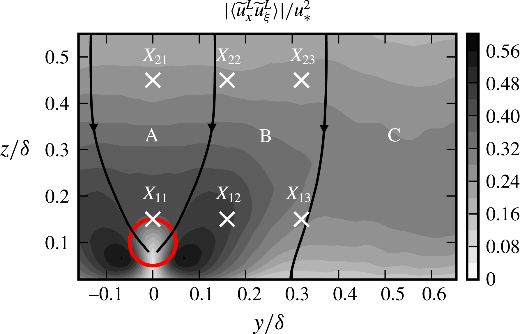
in § 4.2 suggested three distinct dynamic regions in the flow: a passive zone in the upper part of the wake region and above (zone A) where large-scale turbulent quantities are relatively small compared to their environment, an active zone in lateral directions around the wake (zone B) where large-scale turbulent transport and energy is more intense and the far field (zone C) where the fields return to their standard unperturbed ABL distributions. This decomposition is indicated in figure 12 using contours of
 $\langle \widetilde{u}_{x}^{L}\widetilde{u}_{\unicode[STIX]{x1D709}}^{L}\rangle$
at
 $x=8.5S_{x}$
. In this figure, suitable instances of large-scale flux lines, lines parallel to
 $\unicode[STIX]{x1D731}^{L}$
, are employed to separate the dynamic zones.
Location of the event points at transverse plane
 $x=5.95\unicode[STIX]{x1D6FF}=8.5S_{x}$
. Two more event points are selected in the far unperturbed field at
 $\boldsymbol{x}_{14}=(5.95\unicode[STIX]{x1D6FF},2\unicode[STIX]{x1D6FF},0.15\unicode[STIX]{x1D6FF})$
and
 $\boldsymbol{x}_{24}=(5.95\unicode[STIX]{x1D6FF},2\unicode[STIX]{x1D6FF},0.45\unicode[STIX]{x1D6FF})$
to provide baseline cases.

We select two points in the passive zone, four points in the active zone and two reference points in the far field. The event points
 $\boldsymbol{x}_{p}$
are located on a
 $2\times 4$
grid at two different heights
 $z_{1}=0.15\unicode[STIX]{x1D6FF},z_{2}=0.45\unicode[STIX]{x1D6FF}$
, and four different lateral positions
 $y_{1}=0$
,
 $y_{2}=0.16\unicode[STIX]{x1D6FF}$
,
 $y_{3}=0.32\unicode[STIX]{x1D6FF}$
,
 $y_{4}=2\unicode[STIX]{x1D6FF}$
. The positions of the event points around the row are shown in figure 12. The subscripts of the points are named after their positions on the grid where the first subscript refers to the rank in the vertical direction and the second refers to the rank in the horizontal direction, e.g.
 $\boldsymbol{x}_{23}=(5.95\unicode[STIX]{x1D6FF},z_{2},y_{3})$
.
5.2 Conditional eddies
In this section, we conduct a conditional analysis on VLSMs. We start our analysis with large-scale low-velocity events that are defined on an event point
 $\boldsymbol{x}_{p}$
, i.e.
 $$\begin{eqnarray}E_{p}^{l}:=(\widetilde{u}_{x}^{L}(\boldsymbol{x}_{p})<0),\end{eqnarray}$$
and apply ensemble averaging to large-scale fluctuating velocity fields conditioned on these events, i.e.
 $\langle \widetilde{\boldsymbol{u}}^{L}|E_{p}^{l}\rangle$
. We refer to these fields as conditional eddies
 ${\mathcal{E}}_{p}^{l}$
, and will study their geometry, size, topology and transport properties. The superscript
 $l$
in
 $E_{p}^{l}$
and
 ${\mathcal{E}}_{p}^{l}$
is used to imply the low-velocity event.
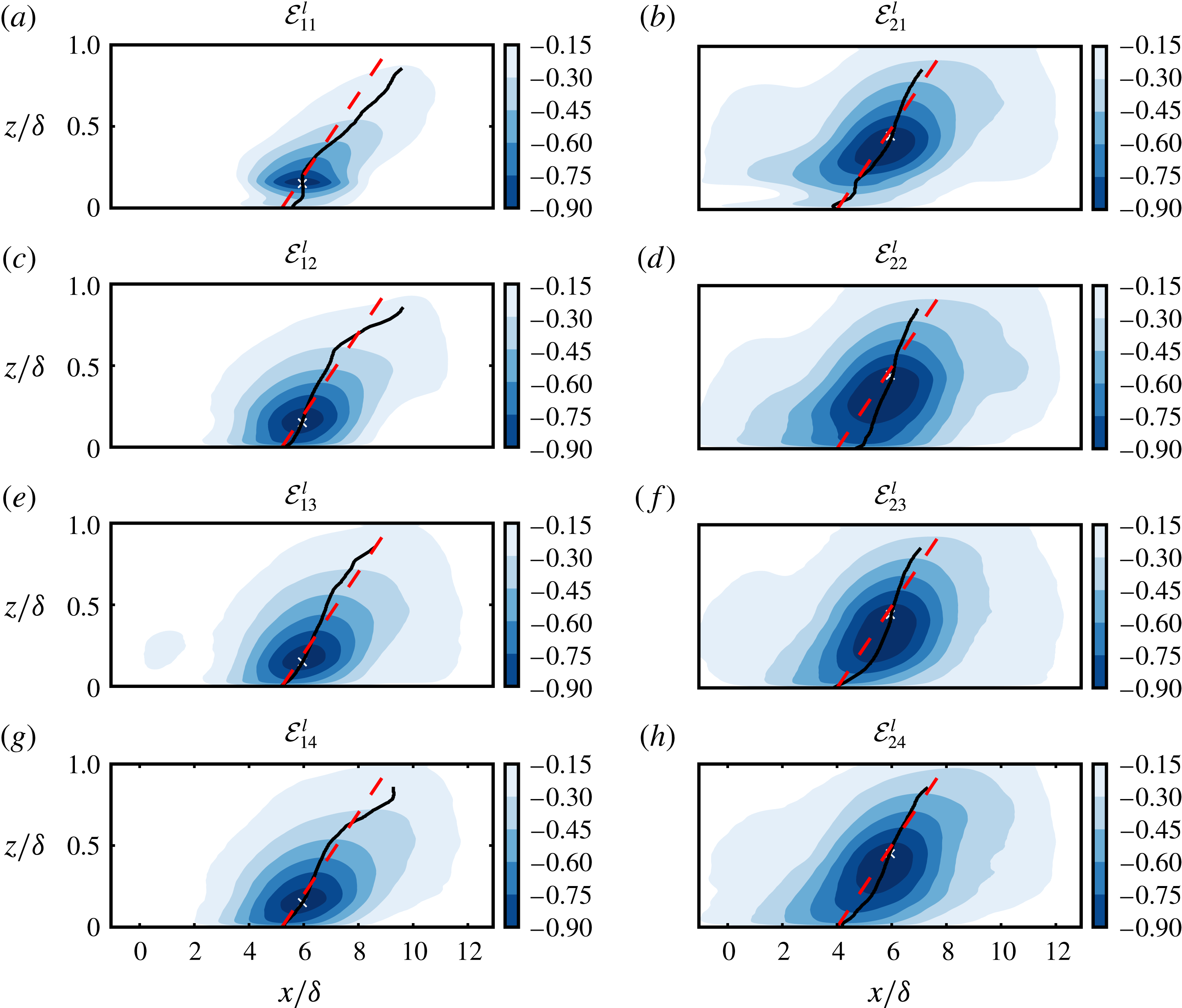
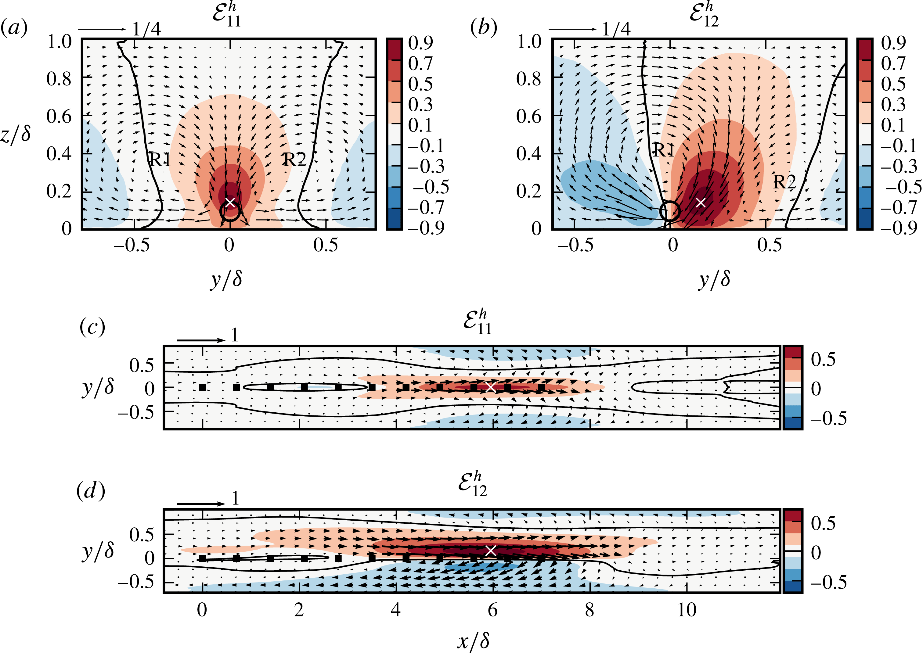
Side view of conditional eddies
 ${\mathcal{E}}_{p}^{l}$
at
 $y=y_{p}$
, cf. figure 12. Eddies are calculated using large-scale low-velocity events
 $E_{p}^{l}:=\widetilde{u}_{x}^{L}(\boldsymbol{x}_{p})<0$
. Filled contours are the normalized streamwise components
 $\langle \widetilde{u}_{x}^{L}|E_{p}^{l}\rangle /\langle \widetilde{u}_{x}^{L}(\boldsymbol{x}_{p})|E_{p}^{l}\rangle$
. Markers show the location of the event points
 $\boldsymbol{x}_{p}$
. Dashed lines show
 $14^{\circ }$
inclination angle. Solid lines mark the position of minimum conditional streamwise velocity at each height.

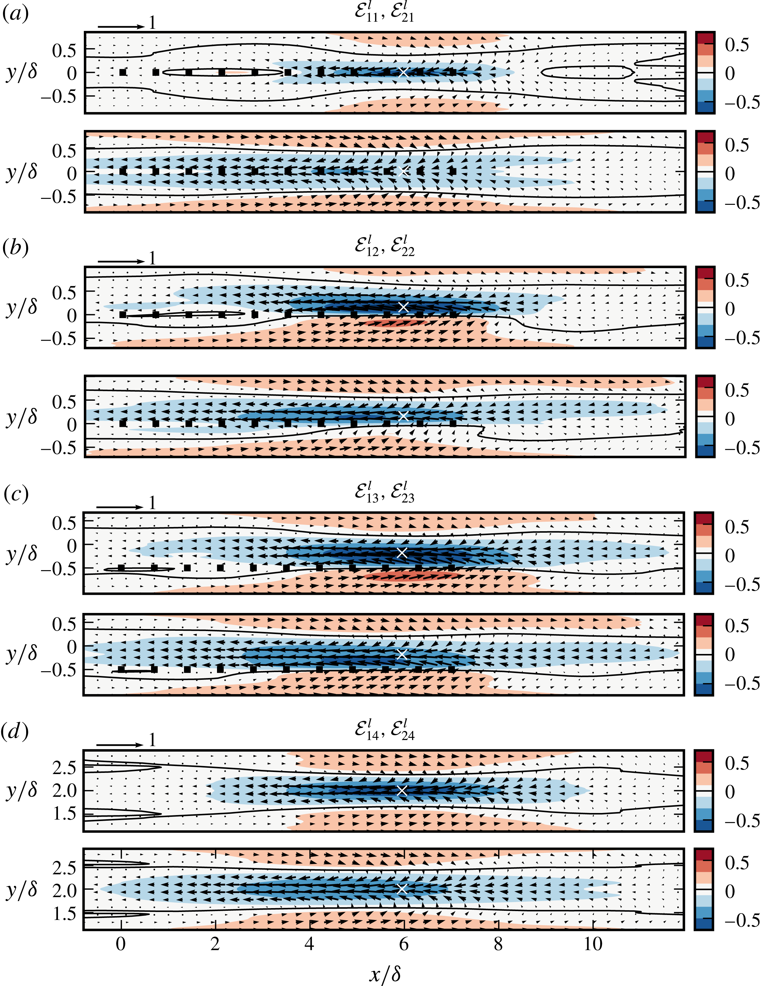
Horizontal view of conditional eddies
 ${\mathcal{E}}_{p}^{l}$
at hub-height
 $z/\unicode[STIX]{x1D6FF}=0.1$
. Eddies are calculated using large-scale low-velocity events
 $E_{p}^{l}:=(\widetilde{u}_{x}^{L}(\boldsymbol{x}_{p})<0)$
on
 $\boldsymbol{x}_{p}$
, cf. figure 12. Filled contours are the normalized streamwise components
 $\langle \widetilde{u}_{x}^{L}|E_{p}^{l}\rangle /\langle \widetilde{u}_{x}^{L}(\boldsymbol{x}_{p})|E_{p}^{l}\rangle$
. Arrows demonstrate in-plane velocity vectors
 $(\langle \widetilde{u}_{x}^{L}|E_{p}^{l}\rangle \hat{\boldsymbol{e}}_{x}+\langle \widetilde{u}_{y}^{L}|E_{p}^{l}\rangle \hat{\boldsymbol{e}}_{y})/\langle \widetilde{u}_{x}^{L}(\boldsymbol{x}_{p})|E_{p}^{l}\rangle$
. White markers show the projected location of event points
 $\boldsymbol{x}_{p}$
onto the planes.

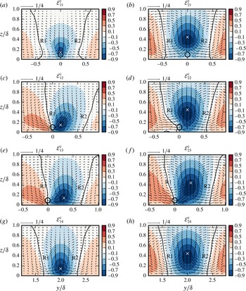
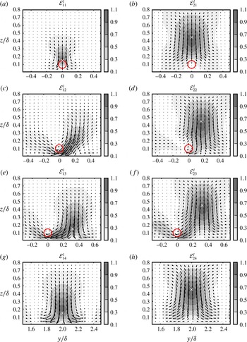
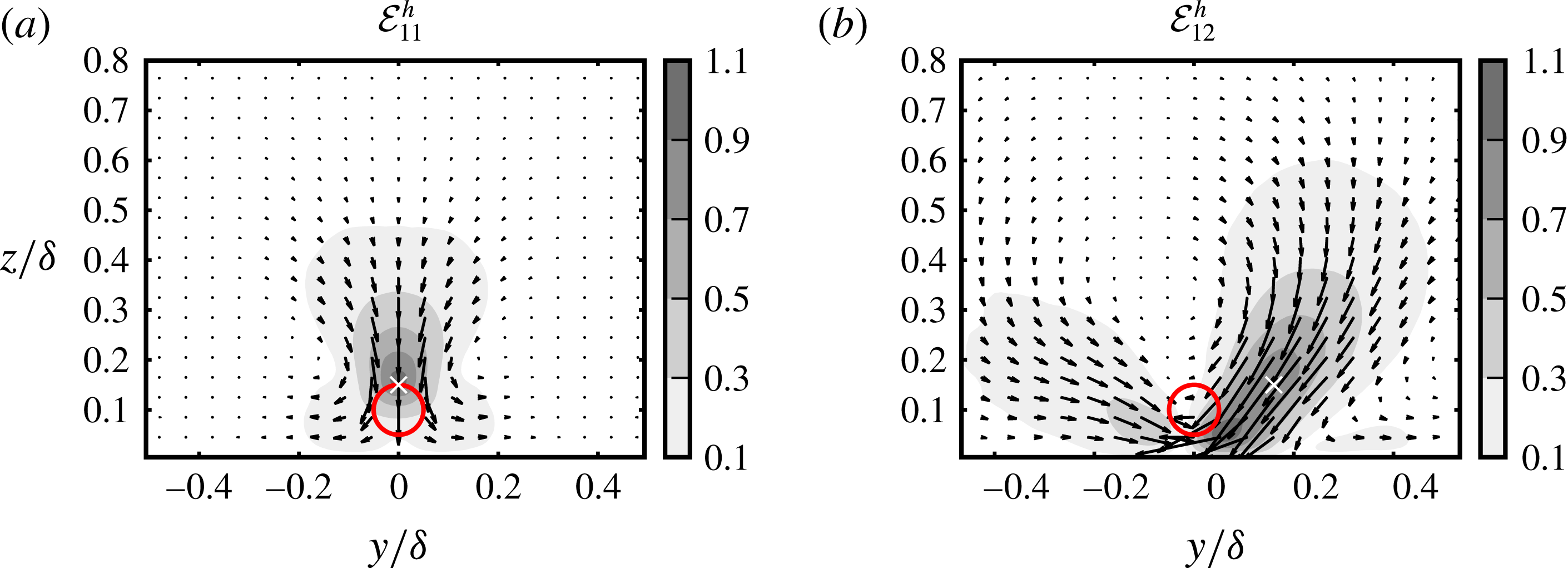
Transverse view of conditional eddies
 ${\mathcal{E}}_{p}^{l}$
at
 $x_{p}=8.5S_{x}$
. Eddies are calculated using large-scale low-velocity events
 $E_{p}^{l}:=(\widetilde{u}_{x}^{L}(\boldsymbol{x}_{p})<0)$
on
 $\boldsymbol{x}_{p}$
, cf. figure 12. Filled contours are the normalized streamwise components, i.e.
 $\langle \widetilde{u}_{x}^{L}|E_{p}^{l}\rangle /\langle \widetilde{u}_{x}^{L}(\boldsymbol{x}_{p})|E_{p}^{l}\rangle$
. Arrows demonstrate normalized in-plane velocity vectors
 $(\langle \widetilde{u}_{y}^{L}|E_{p}^{l}\rangle \hat{\boldsymbol{e}}_{y}+\langle \widetilde{u}_{z}^{L}|E_{p}^{l}\rangle \hat{\boldsymbol{e}}_{z})/\langle \widetilde{u}_{x}^{L}(\boldsymbol{x}_{p})|E_{p}^{l}\rangle$
, which reveal the double-roller structure with rollers R1 and R2. Markers show the location of event points
 $\boldsymbol{x}_{p}$
. The circles demonstrate the projected location of turbines onto the planes.

The conditional fluctuating velocity fields normalized with the reference values at event points, i.e.
 $\langle \widetilde{\boldsymbol{u}}^{L}|E_{p}^{l}\rangle /\langle \widetilde{u}_{x}^{L}(\boldsymbol{x}_{p})|E_{p}^{l}\rangle$
, are shown in figures 13–15. We first investigate the baseline conditional eddies located in the far field and extracted by conditional averaging of events
 $E_{14}^{l}$
and
 $E_{24}^{l}$
. Figure 13(g,h) shows the side views of the conditional eddies using
 $\langle \widetilde{u}_{x}^{L}|E_{p}^{l}\rangle /\langle \widetilde{u}_{x}^{L}(\boldsymbol{x}_{p})|E_{p}^{l}\rangle$
in the
 $x$
–
 $z$
plane at
 $y=2\unicode[STIX]{x1D6FF}$
. These eddies largely correspond to different perspectives of the same coherent structure extending from the surface layer to the outer boundary of the ABL, cf. Sillero, Jiménez & Moser (Reference Sillero, Jiménez and Moser2014) for similar interpretations using two-point correlation maps. The structure has a wall-attached low-momentum zone with a ramp-like inclination. The structure-inclination angle can be estimated by connecting the minimum
 $\langle \widetilde{u}_{x}^{L}|E_{p}^{l}\rangle$
at each altitude, cf. the solid lines in figure 13(g,h). The angle is approximately
 $14^{\circ }$
, cf. the dashed lines in figure 13(g,h), and agrees well with the experimentally reported values for neutral boundary layers, cf. e.g. Chauhan et al. (Reference Chauhan, Hutchins, Monty and Marusic2013). The streamwise extent of the structure can be defined using a low value contour of
 $\langle \widetilde{u}_{x}^{L}|E_{p}^{l}\rangle /\langle \widetilde{u}_{x}^{L}(\boldsymbol{x}_{p})|E_{p}^{l}\rangle$
. We followed a similar approach in § 2.3, where we defined the boundaries as weakly correlated regions of
 $R_{xx}=0.05$
(Hutchins & Marusic Reference Hutchins and Marusic2007; Monty et al.
Reference Monty, Stewart, Williams and Chong2007). However, the absence of small scales in the filtered velocity fields leads to longer extents in the conditional fields for this threshold. Therefore, to be consistent with the literature and the previous analysis in § 2.3, we select
 $\langle \widetilde{u}_{x}^{L}|E_{p}^{l}\rangle /\langle \widetilde{u}_{x}^{L}(\boldsymbol{x}_{p})\rangle =-0.15$
as the boundary threshold. Conditional eddies represent the underlying coherent structure more successfully in their central portions close to their respective event points – far fields are more affected by the statistical smearing and statistical uncertainties due to finite sampling. In this regard, we see that the baseline structure has a streamwise extent of
 $l_{x}\approx 9\unicode[STIX]{x1D6FF}$
at
 $z/\unicode[STIX]{x1D6FF}=0.15$
(cf. the eddy
 ${\mathcal{E}}_{14}^{l}$
in figure 13
g), and
 $l_{x}\approx 13\unicode[STIX]{x1D6FF}$
at
 $z/\unicode[STIX]{x1D6FF}=0.45$
(cf. the eddy
 ${\mathcal{E}}_{24}^{l}$
in figure 13
h). These values are consistent with the reported values in figure 3, and agree well with the streamwise extent of the very large scales in the LES study of Fang & Porté-Agel (Reference Fang and Porté-Agel2015) on neutral ABL.
The horizontal cuts at hub height
 $z=0.1\unicode[STIX]{x1D6FF}$
in figure 14(d) show that the low-momentum region of the baseline structure is flanked on both sides with elongated high-momentum regions. The transverse cuts at
 $x_{p}=5.95\unicode[STIX]{x1D6FF}=8.5S_{x}$
in figure 15(g,h) further show that
 $\unicode[STIX]{x1D6FF}$
-scale counter-rotating streamwise rollers R1 and R2 accompany the elongated streaks. The structure is arranged to produce upwashes of low velocity in the central low-momentum region and downwashes of high velocity in the neighbouring streaks. The low-momentum region has an approximate width of
 $l_{y}\approx 0.6\unicode[STIX]{x1D6FF}$
at
 $z/\unicode[STIX]{x1D6FF}\approx 0.15$
(cf. figure 15
g), and
 $l_{y}\approx 0.9\unicode[STIX]{x1D6FF}$
at
 $z/\unicode[STIX]{x1D6FF}\approx 0.45$
(cf. figure 15
h). In summary, large-scale low-velocity events reveal a baseline ABL structure with inclined low-velocity regions extending over
 ${\sim}10\unicode[STIX]{x1D6FF}$
in the streamwise direction and over the entire ABL thickness in the vertical direction. These elongated elements are accompanied by counter-rotating
 $\unicode[STIX]{x1D6FF}$
-scale swirls. Similar structures have been observed in previous statistical studies on coherent VLSMs, e.g. Chung & McKeon (Reference Chung and McKeon2010), Hutchins et al. (Reference Hutchins, Chauhan, Marusic, Monty and Klewicki2012), Fang & Porté-Agel (Reference Fang and Porté-Agel2015).
We now turn to conditional eddies in the neighbourhood of the turbines. The side views at
 $y=y_{p}$
, the horizontal views at hub height
 $z=0.1\unicode[STIX]{x1D6FF}$
and the transverse views at
 $x=5.95\unicode[STIX]{x1D6FF}=8.5S_{x}$
are shown in figures 13(a–f), 14(a–c) and 15(a–f), respectively. We see that the eddies in the passive zone,
 ${\mathcal{E}}_{11}^{l}$
and
 ${\mathcal{E}}_{21}^{l}$
, have similar organization compared to baseline eddies. However, the cores of these eddies, i.e. the regions with
 $\langle \widetilde{u}_{x}^{L}|E_{p}^{l}\rangle /\langle \widetilde{u}_{x}^{L}(\boldsymbol{x}_{p})|E_{p}^{l}\rangle <-0.3$
, adapt to the mean shear field (cf. figure 7
a), and become attached to the wakes instead of the ground, cf. the contours at
 $z/\unicode[STIX]{x1D6FF}\approx 0.15$
in figures 13(a,b) and 15(a,b). Moreover, there is a reduction in the streamwise lengths in the wake regions compared to the baseline structure, cf. compare the lengths in figure 13(a) to the ones in figure 13(g). This observation suggests that the VLSMs that are directly moving over the turbine row become slightly smaller due to interaction with the turbines.
The turbine row has more significant effects on VLSMs in the active zone as shown by the eddies
 ${\mathcal{E}}_{12}^{l},{\mathcal{E}}_{22}^{l},{\mathcal{E}}_{13}^{l},{\mathcal{E}}_{23}^{l}$
. These eddies correspond to coherent very-large-scale ABL motions that move with some lateral distance parallel to the turbine row. We see in figures 13(c–f), 14(c–f) and 15(c–f) that the resulting flow patterns are non-trivial in terms of orientation and geometry. Despite these geometrical variations, the main coherent-VLSM topology with streaks and counter-rotating vortex cells is reserved in all cases, and appears to be unaffected by the presence of the turbines.
All active zone eddies are highly asymmetric, cf. figure 15(c–f). The streamwise roll modes are rotated, and the R1 rollers, which go through the wake, are slightly lifted up. There is an increase in the magnitude of the conditional fluctuating streamwise velocities
 $\langle \widetilde{u}_{x}^{L}|E_{p}^{l}\rangle$
around the wake, which is consistent with the increased large-scale streamwise energy sideways of the turbines (cf. figure 10
b). Moreover, we see that one side of the low-momentum streaks is partially attached to the wake. Consequently, the boundary of low-momentum cores shown by the isolines
 $\langle \widetilde{u}_{x}^{L}|E_{p}^{l}\rangle =0$
divides the wakes at their centres. For each eddy, this yields a sharp transition from negative to positive momentum within the wake. Figure 14(c–f) shows that this transition takes place along a significant portion of the turbine row. These results suggest that the turbine row separates the elongated streaks of VLSMs.
We address now the organization of the streamwise-momentum transport by conditional eddies. This is investigated using the magnitude and direction of conditional momentum flux
 $$\begin{eqnarray}\overline{\unicode[STIX]{x1D731}}_{p}^{l}=\langle \widetilde{u}_{x}^{L}|E_{p}^{l}\rangle \langle \widetilde{u}_{y}^{L}|E_{p}^{l}\rangle \hat{\boldsymbol{e}}_{y}+\langle \widetilde{u}_{x}^{L}|E_{p}^{l}\rangle \langle \widetilde{u}_{z}^{L}|E_{p}^{l}\rangle \hat{\boldsymbol{e}}_{z}.\end{eqnarray}$$
These fields can also be interpreted as coherent Reynolds stress distributions. We note that
 $\overline{\unicode[STIX]{x1D731}}_{p}^{l}\neq \langle \unicode[STIX]{x1D731}^{L}|E_{p}^{l}\rangle$
, where
 $\langle \unicode[STIX]{x1D731}^{L}|E_{p}^{l}\rangle =\langle \widetilde{u}_{x}^{L}\widetilde{u}_{y}^{L}|E_{p}^{l}\rangle \hat{\boldsymbol{e}}_{y}+\langle \widetilde{u}_{x}^{L}\widetilde{u}_{z}^{L}|E_{p}^{l}\rangle \hat{\boldsymbol{e}}_{z}$
. In fact,
 $\langle \unicode[STIX]{x1D731}^{L}|E_{p}^{l}\rangle$
contains contributions from incoherent velocity fluctuations, i.e.
 $\widetilde{\boldsymbol{u}}^{L}-\langle \widetilde{\boldsymbol{u}}^{L}|E_{p}^{l}\rangle$
, that are not associated with the streak–roller structure, and therefore not useful to our analysis.
Transport of streamwise momentum by conditional eddies
 ${\mathcal{E}}_{p}^{l}$
at
 $x=8.5S_{x}$
. Arrows show the conditional momentum flux
 $\overline{\unicode[STIX]{x1D731}}_{p}^{l}=\langle \widetilde{u}_{x}^{L}|E_{p}^{l}\rangle \langle \widetilde{u}_{y}^{L}|E_{p}^{l}\rangle \hat{\boldsymbol{e}}_{y}+\langle \widetilde{u}_{x}^{L}|E_{p}^{l}\rangle \langle \widetilde{u}_{z}^{L}|E_{p}^{l}\rangle \hat{\boldsymbol{e}}_{z}$
, and filled contours show their normalized magnitude with the reference values at the corresponding event point. Markers show the location of event points
 $\boldsymbol{x}_{p}$
. The circles demonstrate the projected location of the turbines onto the planes.

For brevity, we will investigate only the transverse transport at the plane
 $x=8.5S_{x}$
. The transport upstream and downstream of this plane diminishes quickly. Figure 16(a–h) shows the normalized flux fields at this position for all conditional eddies. We see that the highest values are concentrated close to event points. This is a bias largely related to one-point conditional averaging. It is further observed that the streak–roller structures make widespread contributions to Reynolds shear stress throughout the ABL. The baseline eddies in figure 16(g,h) show that there is a flux of momentum towards the wall along the centreline of the coherent structure, which is a consequence of its streak–roller topology. There is also spanwise transport, which makes zero net contribution to the Reynolds shear stress due to symmetry. The Reynolds stress distributions are somewhat similar for the eddies in the passive zone, compare the contours in figure 16(a,g), or in figure 16(b,h). However, the conditional stresses in these eddies are slightly weaker than the ones in the baseline eddies, and they are lifted up above the wake region as well.
The picture is very different in the active zone, cf. figure 16(c–f). Here the eddies are strongly asymmetric, where the parts close to the wake, i.e. the side of the roller R1, has considerably larger conditional fluxes than the side of roller R2. Moreover, there is also flux from the other side of the wake. The increased transport from both sides of the wake by the eddies in the active zone can be explained using the observations from figure 15(c–f). We see in these panels that roller R1 keeps its integrity and strength, while the conditional streamwise velocity shows dramatic changes in magnitude and sign within the wake. Consequently, the recirculatory field of roller R1 yields streamwise-momentum transport from both sides to the wake.
Conditional eddies
 ${\mathcal{E}}_{p}^{h}$
calculated with high-velocity events
 $E_{p}^{h}:=(\widetilde{u}_{x}^{L}(\boldsymbol{x}_{p})>0)$
. (a,b) Transverse cuts at
 $x/\unicode[STIX]{x1D6FF}=5.95$
; (c,d) horizontal cuts at hub height
 $z/\unicode[STIX]{x1D6FF}=0.1$
. Filled contours are the normalized streamwise components
 $\langle \widetilde{u}_{x}^{L}|E_{p}^{h}\rangle /\langle \widetilde{u}_{x}^{L}(\boldsymbol{x}_{p})|E_{p}^{h}\rangle$
. Arrows demonstrate in-plane conditional velocity vectors.

We now turn to the interaction of high-momentum streaks with the turbine row. To this end, we average with respect to large-scale high-velocity events that are given by
 $$\begin{eqnarray}E_{p}^{h}:=(\widetilde{u}_{x}^{L}(\boldsymbol{x}_{p})>0).\end{eqnarray}$$
The resulting conditional eddies are shown in figure 17. For reasons of brevity, we present only the eddies
 ${\mathcal{E}}_{11}^{h},{\mathcal{E}}_{12}^{h}$
. The same conclusions apply to the remaining eddies. We see that conditional eddies based on large-scale high-velocity events are approximately equal to the negative counterparts of the eddies in low-velocity events, i.e.
 $\langle \widetilde{\boldsymbol{u}}^{L}|E_{p}^{h}\rangle \approx -\langle \widetilde{\boldsymbol{u}}^{L}|E_{p}^{l}\rangle$
. Namely, very long high-momentum streaks interact with the turbine row in a very similar way to low-momentum streaks. High-momentum cores are drawn into the turbine wakes, where the turbine row acts like a sharp boundary to the streaks of the active zone eddy (cf. figure 17
b,d), or weakens the passive zone eddy (cf. figure 17
a,c). Figure 18 further shows the conditional momentum fluxes by these conditional eddies, i.e.
 $$\begin{eqnarray}\overline{\unicode[STIX]{x1D731}}_{p}^{h}=\langle \widetilde{u}_{x}^{L}|E_{p}^{h}\rangle \langle \widetilde{u}_{y}^{L}|E_{p}^{h}\rangle \hat{\boldsymbol{e}}_{y}+\langle \widetilde{u}_{x}^{L}|E_{p}^{h}\rangle \langle \widetilde{u}_{z}^{L}|E_{p}^{h}\rangle \hat{\boldsymbol{e}}_{z}.\end{eqnarray}$$
It is observed that the organization of streamwise-momentum transport by eddies
 ${\mathcal{E}}_{p}^{h}$
is almost identical to the one by eddies
 ${\mathcal{E}}_{p}^{l}$
, i.e.
 $\overline{\unicode[STIX]{x1D731}}_{p}^{h}\approx \overline{\unicode[STIX]{x1D731}}_{p}^{l}$
(cf. figure 16
a,c).
Transport of streamwise momentum by conditional eddies
 ${\mathcal{E}}_{p}^{h}$
at
 $x=8.5S_{x}$
. Arrows show the conditional momentum flux
 $\overline{\unicode[STIX]{x1D731}}_{p}^{h}=\langle \widetilde{u}_{x}^{L}|E_{p}^{h}\rangle \langle \widetilde{u}_{y}^{L}|E_{p}^{h}\rangle \hat{\boldsymbol{e}}_{y}+\langle \widetilde{u}_{x}^{L}|E_{p}^{h}\rangle \langle \widetilde{u}_{z}^{L}|E_{p}^{h}\rangle \hat{\boldsymbol{e}}_{z}$
, and filled contours show their normalized magnitude with the reference values at the corresponding event point.

The visualizations in this section suggest the following scenario for the interaction of VLSMs and wind turbines. When VLSMs move over the wind turbines with a small spanwise distance between their centres and the turbine row, their wall-attached portions strongly interact with the wakes, and eventually dissolve. Their structure then evolves to a slightly smaller wake-attached form with the same double-roller topology. The rollers of these wake-attached eddies either lift up the low-momentum fluid in the wake, or transport the high-momentum fluid to the wake. Therefore, there is a positive transport of streamwise momentum towards the wake. However, the momentum flux is not very strong due to presence of the ground limiting the amount of available fluid to transport.
When a VLSM moves along one side of the turbines, i.e. with its centre at least a few turbine diameters away from the symmetry plane
 $y=0$
, the rotational field of its roller over the turbine row brings high-momentum fluid from the ABL to the wake on one side, and pushes the less energetic wake fluid towards the core of the low-momentum streak on the other side. Therefore, there is an effective flux of positive momentum from both sides of the wake. Moreover, in this configuration, the whole turbine row pushes the elongated streaks aside such that a large portion of the streak resides on one side of the row. This gives rise to an alternating streaky pattern around the turbine row, which is the essential element behind the two-way momentum transport towards the wake.
In summary, VLSMs and their coherent morphology play an active role in the transport of streamwise momentum around the turbine row, which creates the large-scale active and passive zones defined in § 5.1. Moreover, sharp velocity variations within the wake regions of VLSMs in the active zone suggest a role for VLSMs on eccentric loading of wind turbines, where they could contribute out of plane bending moments. This may be interesting to investigate further in the future.
6 Summary and discussion
A kinematic study was conducted to analyse the interaction of a wind turbine row with very-large-scale motions in a neutrally stratified ABL. The analysis was based mainly on two steps. First, the details of Reynolds-averaged transport and energy were investigated using a two-scale decomposition, and the role of very-large-scale ABL motions in laterally inclined momentum and energy distributions were shown. Subsequently, the average form of coherent VLSMs was extracted using conditional sampling on large-scale streamwise-velocity events, and their geometrical modifications were linked to large-scale organization of turbulence around the turbine row.
We studied the statistics of VLSMs by low-pass filtering our LES database at a streamwise cutoff wavelength
 $\unicode[STIX]{x1D706}_{x}=5\unicode[STIX]{x1D6FF}=50D$
. Large-scale Reynolds stresses showed that the effect of very-large-scale motions around the turbine row extend approximately
 $5D$
in lateral directions, and approximately
 $4D$
in the vertical direction. The highly inhomogeneous distribution of the fields suggested two different turbulent transport regimes around the wake. There is a passive zone in the upper part of the wake and above, where the large-scale turbulence activity is relatively smaller than the neighbouring regions on the side of the turbine row, denoted as active zones. We further showed that very-large-scale ABL elements are a relevant part of the flow in the wake region, as they contain approximately
 $20\,\%$
of the resolved Reynolds shear stress, and
 $30\,\%$
of the resolved streamwise kinetic energy in the free-shear layer of the wake region.
In order to link the large-scale turbulence statistics to coherent very-large-scale turbulent structures, we extracted the statistical geometry of VLSMs using one-point conditional averaging based on low-pass filtered streamwise-velocity events. To this end, we selected various points around the turbine row and far in the ABL at
 $z=0.15$
, and
 $z=0.45\unicode[STIX]{x1D6FF}$
. All the conditional eddies appear in the form of very long (
 ${\sim}10\unicode[STIX]{x1D6FF}$
) and wide (
 ${\sim}\unicode[STIX]{x1D6FF}$
) streak–roller structures. Although they share the same topology, the eddies around the turbine row are heavily modified, and have significantly different geometry. For these eddies, turbine wakes act as a momentum sink, and entrain the turbulent structures close to them. As a result, these eddies become partially attached to turbine wakes instead of the ground. This effect yields a remarkable velocity distribution for the eddies in the active zone, where the turbine row to a great extent separates the large-scale elongated streaks. Consequently, high lateral gradients of streamwise velocity are created in the wake regions along the turbine row.
The results of the conditional analysis also provided a new perspective for the turbulent transport around the turbines, and suggested the following scenario. Depending on their relative spanwise location,
 $\unicode[STIX]{x1D6FF}$
-scale swirls can increase either vertical or sideways transport of streamwise momentum. The former is less effective due to the ground limiting the amount of vertically transported fluid, while the latter brings energetic air from high-momentum streak into the wake, and pushes the less energetic wake fluid towards the core of low-momentum streak, hence creating a double-way flux towards the wakes from both lateral directions. These observations shed some light on the mechanisms giving rise to the two distinct large-scale transport zones around the turbine row, which we denoted as passive and active zones above.
The present work studied the interaction of VLSMs and wind turbines in a basic setting where a row of turbines was aligned to the flow direction. It is of great practical interest to see how this interaction would take place in different configurations such as aligned or staggered wind farm layouts. This is an interesting topic of future research. Another limitation of our study was the simplification of boundary conditions in the simulation set-up. In particular for low boundary layers, effects related to temperature stratification and wind veer near the capping inversion may start influencing the structure of VLMSs, potentially leading to additional physics and complexity in the interaction between VLMSs and wind farms.
Acknowledgements
A.Ö. thanks J. P. Goit and W. Munters for useful discussions. The authors acknowledge support from the European Research Council (FP7-Ideas, grant no 306471). The computational resources and services used in this work were provided by the VSC (Flemish Supercomputer Center), funded by the Research Foundation – Flanders (FWO) and the Flemish Government, department EWI.