2.1. Experimental set-up and data acquisition

Experiments are conducted using a generic swirling jet set-up, shown schematically in figure 2, together with the measurement devices used. It consists of an adjustable radial swirl generator that is supplied at four azimuthal positions by regulated air from a pressure reservoir. Several grids ensure a homogeneous distribution of the supplied air. The swirling air is guided normally to the swirler plane in a circular duct of 150 mm diameter followed by a contoured contraction reducing the diameter to $D=51\ \textrm {mm}$. The jet is emanating into a large space (4 m wide, 3 m high) that constitutes unconfined boundary conditions in radial and streamwise directions. Further details of the experimental set-up can be found in Rukes et al. (Reference Rukes, Sieber, Paschereit and Oberleithner2015) and Müller et al. (Reference Müller, Lückoff, Paredes, Theofilis and Oberleithner2020).

Figure 2.

Schematic of the experimental set-up and the utilised measurement systems: HS PIV, high-speed particle image velocimetry; AMP, amplifier; DAQ, data acquisition system. The magnified picture of the flow field is an experimental smoke visualisation of the jet.

The jet is investigated at a fixed mass flow rate of 50 kg h$^{-1}$ that results in a nozzle bulk velocity of $u_{\textit{bulk}} = 5.7$ m s$^{-1}$ and a respective Reynolds number of 20 000 based on the nozzle diameter $D$. The swirl intensity is adjusted by an automated stepper motor that controls the angle of the swirler vanes. Swirl numbers in the range of 0.8 to 1.35 were tested. The current swirl-number definition is based on the linear fit of the integral swirl number against the angle of the swirler vanes. The reason for this approach is due to difficulties with a consistent formulation of the integral swirl number across the investigated swirl range, which is further detailed in Appendix A.

The velocity field of the swirling jet is captured by high-speed (HS) particle image velocimetry (PIV) as indicated in figure 2. A meridional section of the jet is illuminated by the laser and recorded by a high-speed camera. The flow is seeded by silicone-oil droplets (bis(2-ethylhexyl) sebacate; DEHS) of a nominal diameter smaller than 5 mm, which are added to the air between the mass flow controller and the swirler. For each configuration, a set of 2000 images was recorded at a rate of 1 kHz. The images were processed with PIVview (PIVTEC GmbH) using standard PIV processing (Willert & Gharib Reference Willert and Gharib1991) enhanced by iterative multigrid interrogation (Soria Reference Soria1996) and image deformation (Huang, Fiedler & Wang Reference Huang, Fiedler and Wang1993).

The HS PIV captured only the axial and radial velocity components, which is sufficient for the determination of coherent structures. The time resolution of the measurement, however, is essential for the later analysis. The computation of the swirl number, however, requires also the mean azimuthal velocity component. It was determined from non-time-resolved stereoscopic PIV measurements conducted in a previous investigation (Rukes et al. Reference Rukes, Sieber, Paschereit and Oberleithner2015).

Together with the PIV acquisition, pressure measurements were conducted. The probes are located at eight positions around the circumference of the nozzle lip, which are referred to in the following as $p_k$ ($k=1,\dots ,8$). The piezoresistive sensors with a range of 1 kPa were amplified with an in-house bridge amplifier and recorded with a 24-bit analogue-to-digital converter at a rate of 2 kHz. The resonance frequency of the sensor tubing system was at 400 Hz, which is acceptable for the conducted investigations, where the oscillations of the dominant mode were in the range of 50–80 Hz. The resonance of the sensor caused an amplification of the signal by 2 % at 50 Hz and 4 % at 80 Hz. Other than the PIV, the pressure was recorded for 60 s to achieve converged statistics. Pressure measurements were conducted in an automated procedure, where the swirler angle was increased in steps of $0.1^{\circ }$ corresponding to ${\rm \Delta} S$ of $4\times 10^{-3}$.

2.2. Identification of coherent structures from measurement data

This section details how the helical mode is identified from the PIV and pressure data. The first part covers the extraction of the dominant coherent structures from the PIV data using spectral proper orthogonal decomposition (SPOD) as described by Sieber, Paschereit & Oberleithner (Reference Sieber, Paschereit and Oberleithner2016b). The method allows for a modal decomposition of the velocity snapshots, reading

(2.1)\begin{equation} \boldsymbol v(\boldsymbol x,t) = \bar{\boldsymbol v}(\boldsymbol x) + \boldsymbol v'(\boldsymbol x,t) = \bar{\boldsymbol v}(\boldsymbol x) + \sum_{i=1}^{N}{a_{i}(t)\varPhi_{i}(\boldsymbol x)}, \end{equation}

where the fluctuating part of the velocity field $\boldsymbol v'$ is expressed as a sum of spatial modes $\varPhi$ and time coefficients $a$. The used variant of SPOD provides a time-domain representation of the decomposition, which is essential for the present analysis of flow dynamics. This is in contrast to a related frequency-domain representation (Towne, Schmidt & Colonius Reference Towne, Schmidt and Colonius2018), which is not applicable here.

SPOD has promising potential for the analysis of time-domain phenomena in turbulent flows (Noack et al. Reference Noack, Stankiewicz, Morzyński and Schmid2016). This has been shown for the identification of dynamics in the flow of a separated airfoil (Ribeiro & Wolf Reference Ribeiro and Wolf2017), the transient interaction and switching between different dynamics in a combustor (Stöhr et al. Reference Stöhr, Oberleithner, Sieber, Yin and Meier2018), or the provision of proper dynamics for the autonomous modelling of flow dynamics (Lui & Wolf Reference Lui and Wolf2019). The principal advantage of SPOD in these applications is that the dynamics are separated according to their space–time coherence while the time information is maintained, allowing the time-domain analysis of the individual dynamics.

SPOD is based on the snapshot POD proposed by Sirovich (Reference Sirovich1987), with the extension that the snapshot correlation matrix

(2.2)\begin{equation} {\mathsf{R}}_{i,j} = \frac{1}{N} \langle \boldsymbol v'(\boldsymbol x,t_i),\boldsymbol v'(\boldsymbol x,t_j) \rangle \end{equation}

is filtered, which constrains the spectral bandwidth of the coefficients (here $\langle \cdot ,\cdot \rangle$ indicates the $L_2$ inner product; see also Sieber et al. (Reference Sieber, Paschereit and Oberleithner2016b)). The advantage of this approach against spectral filtering of data before or after performing POD is that the filtering is implicitly handled by the decomposition. Hence, there is no need to specify central frequencies of individual phenomena within the data or to apply digital filters. Instead, only the filter width $N_f$ must be chosen, as it sets the bandwidth of the coefficients. The filter is implemented as a simple convolution filter of the snapshot correlation matrix

(2.3)\begin{equation} {\mathsf{S}}_{i,j} = \sum_{k={-}N_f}^{N_f}{g_k {\mathsf{R}}_{i+k,j+k}}, \end{equation}

where $g_k$ is a Gaussian filter kernel. Other than the snapshot POD, SPOD needs time-resolved data to allow time-domain filtering of the data. Further details on the selection of the filter size and handling of boundary conditions can be found in Sieber et al. (Reference Sieber, Paschereit and Oberleithner2016b) and Sieber, Paschereit & Oberleithner (Reference Sieber, Paschereit and Oberleithner2017). Beyond the application of the filter to the correlation matrix, the procedure is the same as for the snapshot POD. In the present investigation, a filter width $N_f$ of two times the oscillation period is used.

For further analysis, the link of mode pairs in the decomposition is identified from a cross-spectral correlation among all possible pairs of coefficients (harmonic correlation as in Sieber et al. (Reference Sieber, Paschereit and Oberleithner2016b)). The appearance of coherent structures as pairs is commonly observed in the POD of real-valued input data. It can be understood as the real and imaginary parts of a mode that is obtained from a spectral analysis. In the following, mode pairs (e.g. SPOD modes 1 and 2) are treated as one mode and they are coupled for the time-domain analysis as the real and imaginary parts of a complex coefficient, $A(t) = a_1(t) + \textrm {i} a_2(t)$.

In the present application, the pressure measurements are used for the dynamic modelling since they allow much longer time series resulting in better-converged statistics than the PIV snapshots. The agreement of mode amplitudes determined from PIV and pressure measurements is detailed in Appendix B. To obtain the mode amplitude, the pressure measurements from the eight positions around the nozzle lip are decomposed azimuthally into Fourier modes, according to

(2.4)\begin{equation} \hat{p}_m(t) = \tfrac{1}{8}\sum_{k=1}^{8} p_k(t) \exp({-\textrm{i} m k {\rm \pi}/4 }) , \end{equation}

where $m$ indicates the azimuthal mode number. The instantaneous amplitude of the helical mode with azimuthal wavenumber $m=1$ is then given as $A(t) =\hat {p}_1(t)$, accounting for the single-helical shape of this coherent structure. The signal was filtered around the average oscillation frequency of the helical mode $f_o$ in the band $[\frac {2}{3}\,f_o,\ \frac {3}{2}\,f_o]$. To set the centre of the filter band, the frequency of the mode was identified from the peak in the unfiltered spectrum and also compared to the frequency of the SPOD coefficients from the PIV measurements. In the low-swirl regime where no peak was visible, the frequency was extrapolated from larger swirl numbers.

In addition to the oscillatory mode, the dynamics of the slowly varying contributions to the flow are obtained from the pressure measurements. They are represented by the shift-mode that is determined from the $m=0$ pressure mode: $B(t) = \hat {p}_0(t)$. Thereby, a relation between the mean flow and the mean pressure is assumed, which is supported by the data shown in Appendices A and B. The $\hat {p}_0$ signal is low-pass-filtered at $4f_o$ to remove acoustic perturbations from the upstream duct. All pressure signals are normalised by the maximum amplitude of the helical mode, this being 6 Pa, to ease the numerical procedures and improve the readability of graphs. The normalisation is not related to the dynamic pressure, which would be around 20 Pa in the present case.

2.3. Flow field and dominant coherent structures

The mean flow field and the structure of the global mode in the swirling jet are sketched in figure 3. Owing to vortex breakdown, the flow forms an annular jet with inner and outer shear layers. The global mode manifests in the central vortex of the jet that meanders and wraps around the breakdown bubble in a helical shape. The rollup of the outer shear layer is synchronised with this motion, resulting in a secondary helical vortex. These co-winding helical vortices cause a spiralling, flapping motion of the annular jet. With respect to the mean flow, the helical vortices are co-rotating and counter-winding. In the current section, the global mode is referred to as the helical mode, in contrast to secondary dynamics that is also observed in the data. The helical mode is considered as the oscillatory mode in the amplitude equation.

Figure 3.

Schematics of the flow field of a swirling jet: (a) streamlines of the mean velocity field coloured by velocity magnitude; (b) slice through the symmetry axis of the mean velocity field represented by sectional streamlines and velocity magnitude as grey contour levels; and (c) instantaneous velocity field indicated by sectional streamlines and coherent structure as grey background. Specific features of the flow fields are marked and indicated in the legends. The breakdown bubble is indicated by the recirculating flow in the centre.

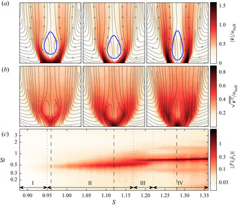
The velocity field and pressure spectra across the investigated swirl range are collectively presented in figure 4. The velocity is normalised with the bulk velocity and the frequency is normalised with the bulk velocity and nozzle diameter to obtain Strouhal numbers as ${St} ={f_o D}/{u_{\textit{bulk}}}$.

Figure 4.

Mean flow and spectrum of the dominant oscillatory mode at different swirl numbers. (a) Contours of relative velocity magnitude together with streamlines; the thick blue line indicates zero axial velocity. (b) The relative turbulence intensity as contours together with streamlines. (c) The magnitude of the spectrum of the pressure Fourier mode $\hat {p}_1$ with a log scaled colour map for all investigated swirl numbers across the relevant Strouhal-number range. The dashed vertical lines indicate the respective swirl number ($S=[0.96,1.12,1.28]$) of the mean flow plots above. The arrows and vertical dotted lines indicate different regimes in the swirl-number range.

The mean velocity fields (figure 4a) show typical features of a swirling jet undergoing vortex breakdown as sketched in figure 3. From the low- to the medium-swirl-number case, there is only little change of the velocity field. The breakdown bubble mainly moves upstream closer to the nozzle in connection with an increased jet spreading. At large swirl number, the breakdown bubble becomes narrower and longer, while the jet spreading decreases.

The turbulence intensity (figure 4b) constantly increases with the swirl strength. The peak intensity is concentrated in the shear layers, while the value at the upstream stagnation point is always the largest. With increasing swirl, the shear layers become thicker and the fluctuations become spread over a larger area.

Several different regimes are visible from the spectrum of the helical mode (figure 4c). Starting from low swirl, there is a range where no oscillations are observed. At swirl numbers of approximately 0.95, there is a slight peak in the spectrum at Strouhal numbers around 0.5. With increasing swirl, the intensity of the peak increases as well as the frequency. Throughout the range, the spectral peak is rather broad. At a swirl number of 1.17, a second, narrow peak at slightly higher frequency appears, which continues to grow while the previous one fades out. After the first peak disappeared at a swirl number of 1.22, the second peak further grows and the frequency increases slightly. At the upper end of the range, the Strouhal number is at 0.73.

Based on the characteristics of the pressure spectra, the investigated swirl range can be divided into four regimes, as indicated in figure 4(c). Regime I corresponds to the swirl range where no helical-mode dynamics is observable. In regime II, the helical mode appears with a broad spectral peak and the mean flow shows a continuous change. Regime III corresponds to a bistable condition. It is characterised by intermittent switching between the states in regimes II and IV, which is visible from time-series data not shown here. Regime IV shows a similar trend as regime II, but with a sharper spectral peak and a longer breakdown bubble.

To provide an overview of the range of dynamics observed in the flow, SPOD is conducted based on flow snapshots acquired at three selected swirl numbers. The cases correspond to the mean velocity fields given in figure 4. The SPOD spectrum presented in figure 5 shows all modes contained in the flow. The detailed picture of spatial structures and coefficient spectra are given for some modes, which are selected such that a consistent ordering is obtained for the different swirl numbers.

Figure 5.

SPOD spectrum (a,c,e) and spatial modes with mode coefficient spectrum (b,d,f) for $S=[0.96,1.12,1.28]$ (from top row to bottom row). The spectrum shows mode energy against Strouhal number, where each dot corresponds to a mode pair and the colour/size indicate the spectral coherence. For selected modes, the spatial and spectral content is detailed as indicated by the numbers. The spatial modes are shown by the transverse velocity (cross-stream in-plane) together with streamlines of the mean flow. The mode coefficients are given as power spectral density.

Figure 5(a,b) shows the SPOD results for the low-swirl case $S=0.96$, which corresponds to the onset of the helical mode. The first SPOD mode (#1) shows a clear peak at $St=0.4$ and the corresponding spatial structure shows typical characteristics of the helical mode (Rukes et al. Reference Rukes, Sieber, Paschereit and Oberleithner2015). Another dominant structure (mode #4) with low frequency ($St=0.05$) is also prominent. It corresponds to an axial movement of the breakdown bubble, as also observed previously by Rukes et al. (Reference Rukes, Sieber, Paschereit and Oberleithner2015). The other inspected modes (#2 and #3) do not indicate clear structures but might be precursors of the dynamics that become more pronounced at higher swirl numbers.

The medium-swirl case $S=1.12$ (figure 5c,d) shows the helical mode again as the most dominant structure (mode #1). There is little change in the mode shape compared to the low-swirl case, but its relative energy increases significantly and it oscillates at a higher frequency of $St=0.5$. There exists another prominent coherent structure at $St=0.3$ (mode #2) that resembles a helical mode in the wake of the breakdown bubble, which has already been observed in combustor flows (Terhaar et al. Reference Terhaar, Reichel, Schrödinger, Rukes, Paschereit and Oberleithner2014; Sieber, Paschereit & Oberleithner Reference Sieber, Paschereit and Oberleithner2016a). The location in the wake and the single helical-mode structure indicates a strong relation to the global mode that is observed in laminar swirling flows, known as spiral vortex breakdown (Ruith et al. Reference Ruith, Chen, Meiburg and Maxworthy2003; Gallaire et al. Reference Gallaire, Ruith, Meiburg, Chomaz and Huerre2006; Qadri, Mistry & Juniper Reference Qadri, Mistry and Juniper2013). In the following, this structure is called the wake mode. At $St=0.8$ there is another mode that slightly sticks out from the continuous spectrum (mode #3). The spatial structure does not exhibit clear symmetries and the coefficient spectrum shows two peaks at $St=0.8$ and $St=1.0$. This mode supposedly represents the helical mode's second harmonic together with an interaction between the wake mode and the helical mode. The mode at very low frequency (mode #4) corresponds to the slowly varying changes of the flow, which is still considerable.

For the high-swirl case $S=1.28$ (figure 5e,f), the mode dynamics is very clear and the low-frequency modes are reduced. The helical mode (#1) at $St=0.69$ has further gained in energy and now clearly exhibits higher harmonics at $St=1.38$ (mode #3) and $St=2.1$. The wake mode (#2) has consolidated at $St=0.36$ and also exhibits a higher harmonic at $St=0.77$ (mode #4). At the frequency of $St=1.05$, where interactions between helical mode and wake mode are expected, there is an agglomeration of less-dominant modes. This indicates an interaction between the two structures, which, however, is not captured by a single mode.

Overall, the SPOD of the flow shows only little change of the helical-mode shape with increasing swirl number. The observed increase in energy and the shift of the oscillation frequency are consistent with the pressure spectra (figure 4). The variations of the mean flow decrease with increasing swirl, which is probably due to the proximity of the breakdown bubble to the nozzle lip at high swirl, which constrains its movement. The SPOD reveals other modes, such as the wake mode and higher harmonics, but the helical mode is most dominant for the entire swirl range. The identified interaction modes remain weak with energies of at least one order of magnitude less than the helical mode. Therefore, the interaction between the helical mode and subdominant modes can be neglected in the following analysis.

3.1. Model design for the stochastic amplitude equation

The form of the presented model is based on the stochastic methods described by Friedrich et al. (Reference Friedrich, Peinke, Sahimi and Reza Rahimi Tabar2011). Accordingly, the stochastic differential equation that describes the temporal evolution of a system has the form of a Langevin equation,

(3.1)\begin{equation} \dot{X} = f(X) + g(X) \xi, \end{equation}

where the dot indicates the time derivative of the state $X$. The deterministic contributions are collected in the drift $f$ and stochastic contributions are covered by the diffusion $g$. The stochastic forcing $\xi$ is Gaussian white noise with vanishing correlation time $\langle \xi (t)\xi (s) \rangle = \delta (t-s)$ (with $\delta$ being the Dirac delta function). The vanishing correlation, which was initially referred to as a Markov process, is essential for the later analysis of the equation.

The amplitude equation serves here as the simplest model to describe the dynamics of the helical mode and the leading-order nonlinearity that governs the saturation at the limit cycle (Stuart Reference Stuart1958; Landau & Lifshitz Reference Landau and Lifshitz1987). It is given as

(3.2)\begin{equation} \dot{A} = (\sigma + \textrm{i}\omega) A - \alpha |A|^2 A + \cdots, \end{equation}

where $A$ is a complex-valued variable that describes the modal coefficient of a periodic perturbation of the flow field. The model parameters are the oscillation frequency $\omega$, the amplification rate $\sigma$ and the Landau constant $\alpha$. Here, no change of frequency due to saturation and no higher-order contributions are considered. A change of the frequency is generally associated with a complex-valued Landau constant, which is assumed to be real for the current investigations. This simplification is justified by the very weak change of the frequency observed in the measurements. Higher-order terms are neglected, since we expect a supercritical Hopf bifurcation, as previously observed by Oberleithner et al. (Reference Oberleithner, Sieber, Nayeri, Paschereit, Petz, Hege, Noack and Wygnanski2011), rather than a subcritical bifurcation, which would require a higher-order model (Meliga, Gallaire & Chomaz Reference Meliga, Gallaire and Chomaz2012a). However, as will be shown, the amplitude equation with cubic saturation remains an approximation of the nonlinearities in the vicinity of the bifurcation point occurring in this flow. In the following, the regime of model applicability will be stretched quite far beyond the bifurcation point to investigate the bounds of this regime.

For the stochastic flow model, noise is added to the amplitude equation (3.2), reading

(3.3)\begin{equation} \dot{A} = (\sigma + \textrm{i}\omega) A - \alpha |A|^2 A + \xi, \end{equation}

where the noise is complex, $\xi = \xi _r + \textrm {i} \xi _i$, with uncorrelated real and imaginary parts, i.e. $\langle \xi _{r}\xi _{i} \rangle =0$. The noise has zero mean and the variance $\varGamma = \overline {\xi \xi ^*}$ (where $^*$ indicates the complex conjugate). A complex-valued noise is necessary to maintain the symmetry of the equation.

The representation of the mode coefficient as amplitude and phase, $A = |A| \ \textrm {e}^{\textrm {i}\phi }$, allows one to separate the unperturbed amplitude equation (3.2) into two simple real-valued equations reading

(3.4a,b)\begin{equation} |\dot{A}| = \sigma|A| - \alpha |A|^3, \quad \dot{\phi} = \omega. \end{equation}

The amplitude and phase are regarded as slow and fast variables, meaning that $|\sigma | \ll |\omega |$. In combination with the amplitude and phase representation, this allows stochastic averaging over the fast variables of the stochastic equation (3.3) (Roberts & Spanos Reference Roberts and Spanos1986), which gives

(3.5)\begin{gather} |\dot{A}| = \sigma |A| - \alpha |A|^3 + \frac{\varGamma}{|A|} + \xi_{A}, \end{gather}

(3.6)\begin{gather}\dot{\phi} = \omega + \frac{\xi_{\phi}}{|A|} . \end{gather}

The conversion results in different contributions of the noise to the amplitude and phase ($\xi _{A}$ and $\xi _{\phi }$) as indicated by the subscripts. These noise contributions are real-valued, uncorrelated, i.e. $\langle \xi _{A}\xi _{\phi } \rangle =0$, and have half the variance of the complex perturbation, i.e. $\langle \xi _{A},\xi _{A} \rangle = \langle \xi _{\phi },\xi _{\phi } \rangle =\varGamma /2$.

The stochastic averaging of the equation refers to a short-term integration of the stochastic contributions that is analogous to previous approaches (Noiray Reference Noiray2017; Lee et al. Reference Lee, Zhu, Li and Gupta2019), where the Van der Pol oscillator instead of the amplitude equation was considered. The Van der Pol oscillator has an equivalent amplitude and phase representation as (3.5) and (3.6), which makes the approaches comparable. The only difference in the present approach is the use of complex noise that maintains the symmetry of the equation even for large amplitudes and strong noise. Further details on the relationship between the two equations are given in Appendix C.

The change of variables separates the model into two equations. The amplitude equation (3.5) is independent of the phase, describing the exponential amplification and saturation mechanism of the oscillatory mode. In the unperturbed case (3.4a,b), the sign of the amplification rate $\sigma$ determines whether the oscillations occur or not. However, the additional deterministic contribution ${\varGamma }/{|A|}$ in the stochastic amplitude equation (3.5) prevents the oscillator from decaying to zero amplitude even for negative amplification rates. In addition to the new deterministic contribution, the additive stochastic perturbation remains in the amplitude equation. Considering the phase equation (3.6), the stochastic forcing causes the phase to be dependent not only on the frequency but also on parametric perturbations that scale inversely with the amplitude. Therefore, the stochastic forcing couples the phase to the amplitude equation.

To estimate the noise intensity from experimental data, the phase equation (3.6) is rearranged to

(3.7)\begin{equation} \xi_{\phi,\textit{est}} = |A| (\dot{\phi} - \omega ), \end{equation}

which can be used to estimate the noise intensity using

(3.8)\begin{equation} \frac{\varGamma_\textit{est}}{2} = \langle \xi_{\phi,\textit{est}},\xi_{\phi,\textit{est}} \rangle . \end{equation}

The extraction of the remaining parameters from the amplitude equation is detailed in the subsequent section.

3.2. Stochastic perturbations with coloured noise

The application of stochastic methods requires the noise to be white (uncorrelated) to obtain a Langevin equation. However, the noise may have a short correlation time, which makes the stochastic forcing coloured instead of white noise. This is reasonable as long as the time scales of the deterministic and stochastic dynamics are well separated (Hänggi & Jung Reference Hänggi and Jung1994). A simple type of coloured noise is obtained from an OU process, which has the autocorrelation

(3.9)\begin{equation} \langle \xi(t),\xi(s) \rangle = \frac{D}{\tau}\exp({-|t-s|/\tau}) \end{equation}

and is created from a basic stochastic process as

(3.10)\begin{equation} \dot{\xi} ={-} \frac{1}{\tau} \xi + \frac{\sqrt{D}}{\tau} \xi_{w}. \end{equation}

In the above equations, $\xi$ denotes the noise created from the OU process with time scale $\tau$ and intensity $D$. The variable $\xi _{w}$ denotes a white noise process with a variance of one that drives the OU process. To incorporate the coloured noise into the stochastic flow model, the specific correlation (3.9) is included in the stochastic averaging of the amplitude equation (Bonciolini et al. Reference Bonciolini, Boujo and Noiray2017; Noiray Reference Noiray2017). Accordingly, it is sufficient to replace the noise intensity in (3.5) by an effective noise intensity

(3.11)\begin{equation} \varGamma_{\tau} = \frac{2D}{\tau^2\omega^2+1} = \frac{2 \tau \langle \xi,\xi \rangle}{\tau^2\omega^2+1}, \end{equation}

which is equivalent to the power spectrum of the OU noise at the oscillator frequency $\omega$. Note that the factor 2 in the equation results from the two noise components in the complex-valued forcing.

The time scale and intensity of the stochastic forcing were estimated from the empirical relation

(3.12)\begin{equation} \langle \xi_\phi(t),\xi_\phi(s) \rangle \approx \frac{D}{2\tau} \exp({|t-s|/\tau}) \cos(\omega (t-s)), \end{equation}

which is obtained by comparing the autocorrelation of the phase distortion (3.7) from a simulated model with coloured noise to the analytical correlation (3.9). By adding the cosine factor to the analytical correlation of the OU process, good agreement with the simulation is obtained (see figure 7). The obtained correlation (3.12) can be interpreted such that the cosine term accounts for the different coordinates in which the noise is represented. The noise adds to the amplitude equation as uncorrelated real and imaginary parts in a fixed coordinate system, whereas the phase distortion is considered in the rotating coordinates of the oscillator. Since the added noise is correlated in time, the rotation of the coordinate system in time must be accounted for in the correlation.

The procedure outlined here, using an effective noise and the estimation of the noise properties from the phase distortion, is only strictly valid for noise time scales that are smaller than the oscillator time scale and for small noise amplitudes. This limit of applicability is further investigated in § 3.4.

3.3. System identification from stationary probability density functions

The method presented here is used to estimate the parameters of the amplitude equation by inspecting the stationary PDF of measured amplitudes. An analytical expression for the stationary PDF is derived from the amplitude equation (3.5) through the corresponding Fokker–Planck equation. Therefore, the amplitude equation is brought in the form of the Langevin equation (3.1), where the corresponding drift and diffusion terms are

(3.13)\begin{gather} f(|A|) = |A| (\sigma - \alpha |A|^2 ) + \frac{\varGamma}{|A|}, \end{gather}

(3.14)\begin{gather}g(|A|) = \sqrt{\varGamma/2}, \end{gather}

respectively. The assumption of a Markov process allows one to describe the temporal evolution of the PDF of the magnitude $|A|$ by the Fokker–Planck equation (Friedrich et al. Reference Friedrich, Peinke, Sahimi and Reza Rahimi Tabar2011),

(3.15)\begin{equation} \frac{\partial}{\partial t}P(|A|,t) ={-}\frac{\partial}{\partial |A|} (\,f(|A|) P(|A|,t) ) + \frac{1}{2} \frac{\partial^2}{\partial|A|^2} ( g^2(|A|) P(|A|,t) ), \end{equation}

where $P$ refers to the PDF. This eliminates the stochastic variable and gives a probabilistic description of the system, which can be compared to statistical moments obtained from measured data.

In order to identify the model parameters, a stationary solution of the Fokker–Planck equation $({\partial }/{\partial t})P(|A|,t) = 0$ has to be found. Following the derivations of Noiray (Reference Noiray2017), the stationary Fokker–Planck equation with vanishing PDF at infinite amplitudes and constant diffusion $g$ simplifies to

(3.16)\begin{equation} \frac{\mathrm{d}}{\mathrm{d} |A|}P(|A|) - \frac{2}{g^2}\,f(|A|) P(|A|) = 0. \end{equation}

The corresponding solution is obtained by writing the drift coefficient in a potential form, reading

(3.17)\begin{equation} f(|A|) ={-}\frac{\partial\mathcal{V}(|A|)}{\partial |A|}\quad \mathrm{with}\ \mathcal{V}(|A|) ={-}\frac{\sigma}{2}|A|^2 + \frac{\alpha}{4}|A|^4 -\varGamma\ln{|A|}, \end{equation}

which gives

(3.18)\begin{equation} P(|A|) = \mathcal{N}\exp\left(-\frac{4}{\varGamma}\mathcal{V}(|A|)\right). \end{equation}

The scale parameter $\mathcal {N}$ is chosen to normalise the PDF such that $\int _0^\infty P(|A|)\,\mathrm {d}|A| = 1$. The expression contains a mixture of stochastic and deterministic parameters that are identified from different measures.

The strategy for the presented analysis is the following. We use a generic model of the PDF,

(3.19)\begin{equation} P_\textit{mod}(|A|) = \mathcal{N} |A| \exp (c_1 |A|^2 + c_2 |A|^4 ), \end{equation}

with the parameters $c_1$ and $c_2$. It is fitted to the experimental PDF $P_\textit{exp}$ using the Kulback–Leibler divergence

(3.20)\begin{equation} D_\textit{KL} = \int_0^\infty {P_\textit{exp}(|A|) \log\left(\frac{P_\textit{exp}(|A|)}{P_\textit{mod}(|A|)}\right)}\,\mathrm{d}|A|\end{equation}

as similarity measure. The divergence $D_\textit{KL}$ is minimised using common numerical procedures. The effective noise intensity $\varGamma _\tau$ is obtained from the procedure described in § 3.2. Together with the fitting parameters of the model PDF, this provides the physical model parameters

(3.21a,b)\begin{equation} \sigma = \frac{c_1\varGamma_\tau}{2} \quad \mathrm{and}\quad \alpha ={-}c_2 \varGamma_\tau , \end{equation}

where the estimation of the amplification rate $\sigma$ is most important for the interpretation of the flow state. Furthermore, the divergence $D_\textit{KL}$ is used to measure if the model fails to approximate the measured dynamics.

For illustrative purposes, figure 6 shows a characteristic time series of an unstable system ($\sigma >0$) and a stable system ($\sigma <0$) that are both subjected to stochastic forcing. The signal was generated by numerical integration of the forced amplitude equation (3.3). The unstable system is initialised at $A=0$ and quickly approaches the limit cycle. Owing to the stochastic forcing, it never settles at the limit cycle. The stationary PDF of the amplitude quantifies the disturbance of the flow state around the limit cycle. The distribution reflects the balance between the stabilising drift that pushes the system to the limit cycle and the destabilising stochastic forcing. This is the same for the stable system, with the difference that the deterministic dynamics of the system tends to zero amplitude but gets continuously excited by the stochastic forcing. The estimation of the model parameters from the stationary PDF and the phase distortion allows one to quantify the balance between these forces and provides estimates of physical amplification rates.

Figure 6.

Exemplary time series of the simulated stochastic amplitude equation (3.3) for an unstable system (a) and a stable system (b). The blue line shows the real part of $A$ and the red line gives the corresponding magnitude $|A|$. The bar blots on the right show the stationary PDF of the magnitude. The models are simulated with white noise, and the ratio $\omega /\sigma$ is 10 for the unstable and $-$10 for the stable case.

3.4. Numerical study of the amplitude equation with coloured noise

The numerical study aims to validate the assumptions made during the derivation of the analytical procedure in §§ 3.1 to 3.3. Especially, the stochastic averaging (3.5) and the estimation of the noise properties (3.12) need to be validated for coloured noise. Therefore, the original complex-valued equation (3.3) is numerically integrated in time with coloured noise from an OU process (3.10). The OU process is integrated with a second-order Runge–Kutta scheme for stochastic equations (Tocino & Ardanuy Reference Tocino and Ardanuy2002). The amplitude equation is integrated with a fourth-order Runge–Kutta scheme with fixed time steps corresponding to 100 steps per oscillation period. The coloured noise is simulated with twice the temporal resolution to allow the Runge–Kutta scheme to be evaluated for intermediate time steps. In the cases with white noise forcing, the amplitude equation is simulated like the OU process. The amplitude equation is simulated for a range of amplification rates $\sigma = -1, \ldots , 1\ \textrm {s}^{-1}$, noise time scales $\tau = 0, \ldots , 1\ \textrm {s}$ and effective noise intensities $\varGamma _{\tau } = 0.01, \ldots , 1$. The frequency is kept constant at $f_o=10$ Hz as well as the Landau constant $\alpha =1$. The parameters of the amplitude equation are identified according to (3.21a,b) and the effective noise intensity according to (3.11) and (3.12).

The fit of the model to the simulation data is exemplified in figure 7 for selected cases. The selection shows an unstable system for different noise time scales but the same effective noise intensity. In figure 7(a), the autocorrelation of the phase distortion is shown. Accordingly, the estimation of the noise parameters from the decay of the correlation envelope works well for small and intermediate noise time scales but deviates for the large noise time scale. Figure 7(b) shows the simulated, estimated and analytically derived amplitude PDFs. Since all presented simulations have the same effective noise intensity and model parameters, the analytic PDF must be the same for all cases (see (3.12)). For the small noise time scale ($\tau =0.01$), all shown PDFs agree very well. For the moderate noise time scale ($\tau =0.1$), the analytical and simulated PDFs deviate slightly. Note that the noise time scale here is of the same order as the oscillation frequency. Therefore, the assumed separation of time scales is no longer met, but, nevertheless, the deviations stay small. The long noise time scale ($\tau =1$) causes significant deviations of the expected and simulated PDFs. Furthermore, the shape of the PDF is not correctly captured by the analytical model, indicating the need for higher-order approximations.

Figure 7.

Selected simulation results of the numerical study at $\sigma =0.5$, $\varGamma _{\tau } = 0.1$ and $\tau = [0.01,0.1,1]$, as indicated in the top-right corner. (a) The noise correlation from the simulation, as well as the estimated and analytical decay (plots are normalised by the value at zero shift $t=s$). The blue dots indicate the local maxima which are used to estimate the decay. (b) The PDF of the envelope calculated from the simulation, the estimated fit to the simulation results and the expected analytical PDF.

The estimated amplification rates and effective noise intensities for all simulated cases are presented in figure 8. The estimated amplification rate is displayed against the rate used in the simulation. For a perfect estimation, the graph displays a straight diagonal, which is the case for the simulation with white noise ($\tau =0$). For $\tau = 0.01$ and $\tau = 0.1$, the relative deviations stay below 10 %; while for $\tau = 1$, the deviations exceed this limit. The source of the error is either an inaccurate fit of the PDF with the model (3.19) or an inaccurate estimation of the noise properties from the empirical correlation function (3.12). To differentiate between these two error sources, the estimates are also shown based on the true noise intensity. Accordingly, the errors from both sources are of the same order of magnitude. For the cases with $\tau \le 0.1$, the error generally only changes the slope of the amplification curve, and the bifurcation point (zero crossing) is accurately captured. With increasing noise time scales, the absolute rate becomes increasingly underpredicted, as seen from the decreasing slope. The estimation for $\tau = 1$ strongly deviates for the PDF fit as well as for the noise estimation. Hence, the model is not able to cover cases with noise time scales larger than the oscillation period $\tau > 1/f_o$.

Figure 8.

Estimates of the model coefficients from the simulation data at $\varGamma _{\tau } = 0.1$ and different noise time scales indicated in the legend. (a) The estimated against the true amplification rate. The solid curves show results with estimated $\varGamma _{\tau }$ and the dashed lines those with true $\varGamma _{\tau } = 0.1$. (b) The corresponding estimation of the effective noise intensity from data.

The numerical study shows that the model and the simplifications made in the deviations are valid as long as the noise time scale stays below the oscillatory time scale. Surprisingly, there is no need for a large separation of time scales if small deviations are acceptable. A perfect agreement, however, is only possible for purely white noise.

3.5. Parameter estimation of the amplitude equation from experiments

This section shows the results from the application of the procedure outlined in §§ 3.1 to 3.3 to the oscillatory mode measured from the pressure Fourier modes (2.4). An overview of the measured PDFs is given in figure 9 and the estimated model parameters are presented in figure 10.

Figure 9.

Analysis of the amplitude statistics derived from pressure measurement. (a) The PDF of the envelope $P(|A|)$ as contours for different swirl numbers. (b) Bar plots of the measurement data together with the best fit of the theoretical PDF as a red line. These plots correspond to sections of the contour plot above, where the corresponding positions are marked as dashed lines. The arrows and vertical dotted lines indicate different regimes in the swirl-number range.

Figure 10.

Estimated model parameters against the swirl number obtained from pressure measurements. (a) The amplification rate; the inset is a vertical zoom into the region around zero. (b) The oscillation frequency $f_o$ together with the noise time scale $\tau$. (c) The divergence (3.20) between the measured and the theoretical PDF (see figure 9). The arrows and vertical dotted lines indicate different regimes in the swirl-number range.

The amplitude PDFs presented in figure 9 show a continuous transition from narrow to wider distributions. A qualitative change can be observed in regime III, where the bistability of the mean flow occurs. The analytical model fits the observed PDF adequately, and larger deviations are only visible in the bistable regime. The gradual change of the PDF and the mean amplitude does not indicate a bifurcation point from this representation.

Figure 10 displays the estimated amplification rate (a), the estimated noise time scale (b) and the deviation of the PDF fit (c) quantified with the Kulback–Leibler divergence. Going through the graphs from low to high swirl, the amplification rate shows first a strong increase from largely negative values up to zero. After the bifurcation at $S=1.1$, the estimated rates stay positive but the curve flattens and stays close to zero before there is a sudden increase in regime III. The noise time scale is always smaller than the oscillation time scale except for regime III. Similarly, a high divergence is observed in this regime, indicating a poor fit quality, whereas the divergence is low for all other swirl intensities. The overall divergence level is lowest in the stable regime and increases a little at $S=1.05$. Overall, the presented model parameters give a clear indication of the bifurcation point and also provide a quantification of the reliability of the estimation.

The estimation results in the bistable regime of the flow appear not to be reliable. This is primarily due to the stochastic switching between the two flow states, which creates low-frequency perturbations of the oscillatory mode that are outside of the model's valid parameter range. This is distinctly indicated by the noise time scale, which becomes larger than the oscillation time scale (figure 10b). The divergence consistently shows the failure of the model in that range. However, the estimated amplification rate does not show large outliers in that region but rather a continuous trend between the two neighbouring regions.

The plateau of the amplification rate at swirl levels slightly above the bifurcation point may be due to the following reasons. Either the decreasing noise time scale causes an underprediction of the estimation, in confirmation with the model study (§ 3.4), or the one-dimensional (1-D) dynamical model oversimplifies the underlying system dynamics at this flow regime. The latter will be addressed in the following section. The entire set of model parameters for the investigated swirl-number range is presented in Appendix D.

4.1. Model design and calibration procedure

In the model described in the previous section, the dynamics of the oscillatory mode is assumed to be independent of other state variables of the flow. However, the interaction of the oscillatory mode with the mean flow might take some time, such that there is a delayed saturation of the amplitude equation. This is further evaluated from an inspection of the mean-flow changes given by the shift-mode, which is referenced by the mode coefficient $B$. The coupled dynamics of the oscillatory mode $A$ and the shift-mode $B$ is described by the mean-field model (Noack et al. Reference Noack, Afanasiev, Morzyński, Tadmor and Thiele2003; Luchtenburg et al. Reference Luchtenburg, Günther, Noack, King and Tadmor2009), which is given as

(4.1)\begin{gather} \dot{A} = (\sigma + \textrm{i}\omega ) A - \beta(B-B_0)A, \end{gather}

(4.2)\begin{gather}\dot{B} ={-}\frac{1}{\tau_B} (B - B_0 - \gamma|A|^2 ), \end{gather}

in the present nomenclature. The dynamics of the oscillatory mode $A$ is very similar to the amplitude equation (3.2), but the saturation $\alpha |A|^2$ is exchanged by the feedback from the shift-mode, $\beta (B-B_0)$. The change of the shift-mode $B$ is driven by the Reynolds stresses induced by the oscillatory mode $\gamma |A|^2$. If there is no oscillatory mode, the mean flow restores to the fixed point $B_0$, commonly called the base flow. The rate of return to the fixed point is given by the time constant $\tau _B$. At the limit of an infinitely short time constant, the shift-mode is slaved to the oscillatory mode as $(B-B_0) = \gamma |A|^2$, and the amplitude equation (3.2) is obtained again, with the Landau constant being $\alpha =\beta \gamma$.

In the present investigation, the mean-field model is adapted to capture the dynamics observed in the experimental data. This results in the following model, where the dimension is reduced similar to the amplitude equation (3.4a,b) by changing variables to the phase–magnitude representation and retaining only the magnitude, yielding

(4.3)\begin{gather} |\dot{A}| = (\sigma - \alpha |A|^2 - \beta(B-B_0) )|A| + \frac{\varGamma}{|A|}, \end{gather}

(4.4)\begin{gather}\dot{B} ={-}\frac{1}{\tau_B} ( B - B_0 - \gamma |A|^2 ), \end{gather}

which describes the evolution of the oscillation magnitude $|A|$ and the shift-mode $B$.

The amplitude equation in the adapted mean-field model (4.3) covers two saturation mechanisms. The first is called ‘direct saturation’ and is represented by the quadratic term $\alpha |A|^2$, which is equivalent to the representation in the amplitude equation (3.2). The second is called ‘delayed saturation’ and is represented by the shift-mode term $\beta (B-B_0)$ introduced in the basic mean-field model (4.1). The inclusion of both mechanisms is necessary to capture the dynamics observed in the data, which is discussed in the following section.

The parameters $\alpha$, $\beta$ and $\gamma$ in (4.3) and (4.4) are positive, which implies only negative feedback. In other words, an increasing amplitude shifts the mean flow to a state that causes less amplitude growth and vice versa. The fixed points of the system of equations lie on an inertial manifold called the mean-field paraboloid, given by $\gamma |A|^2 = B - B_0$ (Noack et al. Reference Noack, Afanasiev, Morzyński, Tadmor and Thiele2003). This is an attracting manifold where the mean-flow state corresponds to the Reynolds stresses induced by the limit-cycle oscillations of the system.

The current mean-field model (4.3) is further adapted by the inclusion of the drift term from the amplitude equation (3.5) that results from the additive noise, reading ${\varGamma }/{|A|}$. This empirical adaptation considers the effect of an additive noise that is not explicitly modelled for the mean-field model. The actual addition of a stochastic forcing would need another independent noise term for the shift-mode and an extensive stochastic averaging to reduce the system to the two slow variables, the magnitude of the oscillatory mode and the shift-mode. Furthermore, there is most probably no simple analytical form for this two-dimensional (2-D) system, which would require a numerical solution of the Fokker–Planck equation (Friedrich et al. Reference Friedrich, Peinke, Sahimi and Reza Rahimi Tabar2011).

To overcome these difficulties, a different approach is pursued that extracts the deterministic drift directly from the statistical moments of the measured data. Therefore, the mean-field model needs to cover only the deterministic dynamics and no stochastic forcing. The drift is identified from a conditional average of the observed state $X$ of the stochastic process (Friedrich et al. Reference Friedrich, Siegert, Peinke, St. Lück, Lindemann, Raethjen, Deuschl and Pfister2000), reading

(4.5)\begin{equation} \tilde{f}(X_k) = \lim_{{\rm \Delta} t \rightarrow 0} \frac{1}{{\rm \Delta} t} \langle X(t+{\rm \Delta} t) - X(t) \rangle|_{X(t) = X_k} , \end{equation}

where $\langle {~}\rangle$ indicates the averaging operation. The function $\tilde {f}(X)$ is an estimate of the drift function that drives the process as given by the Langevin equation (3.1). In the present case, the system state is $X = [|A|,B]^\textrm {T}$ and the drift function $\dot {X} = f(X)$ is (4.3) and (4.4). The conditional average in (4.5) considers the mean drift of all trajectories that passed through a certain point in state space $X_k$, where the drift is approximated by a forward-time finite difference. The limit in (4.5) is only valid for strictly white noise, which is often not given for experimental data (Lehle & Peinke Reference Lehle and Peinke2018) and generally not for turbulent perturbations. Therefore, a fixed interval of one oscillation period was chosen to estimate the drift of the slow variables. Neglecting the limit causes an inaccurate prediction of the drift, but relative differences and trends are still captured. Accordingly, the analysis of the mean-field model constitutes a qualitative study of the relation between oscillatory mode and shift-mode. Therefore, the results are not directly compared to the investigations with the amplitude equation in § 3, and the accuracy of the mean-field model is not studied in detail.

The evaluation of the conditional average in (4.5) requires the subdivision of the state space $X = [|A|,B]^\textrm {T}$ into bins. For this purpose, data-based $k$-means clustering of the state space is pursued. This approach has been shown to be very effective for a statistical description of fluid dynamics (Kaiser et al. Reference Kaiser, Noack, Cordier, Spohn, Segond, Abel, Daviller, Östh, Krajnović and Niven2014). The drift, determined for each cluster centre $X_k$, is fitted to the model (4.3) and (4.4) by tuning the parameters to minimise $\sum _k{(\,\tilde {f}(X_k)-f(X_k))^2}$. A consistent calibration of the parameter $\varGamma$ from the estimated drift function turned out to be ineffective, because in unstable cases it was difficult to distinguish between noise-induced and linearly amplified oscillations. To make the estimation of the noise-induced drift more robust, the parameter $\varGamma$ is determined from the phase distortion (3.8) and scaled with a constant factor $c_{\textit{scale}}$ to adapt it to the drift function. This relation reads as $\varGamma = c_{\textit{scale}} \langle \xi _{\phi ,\textit{est}},\xi _{\phi ,\textit{est}} \rangle$, where the factor $c_{\textit{scale}}$ is calibrated to minimise the global sum of squared differences for all investigated swirl numbers.

4.2. Parameter estimation of the mean-field model from experimental data

The parameters of the stochastic mean-field model (4.3) and (4.4) are determined from the drift coefficients estimated from the pressure measurements of the flow, according to the procedure outlined in § 4.1. The pressure data are processed as described in § 2.2 to obtain the magnitude of the oscillatory mode $|A|$ and the shift-mode $B$. The data are scaled to equal variance to obtain clusters from $k$-means clustering with 100 centres. Throughout the processing, the clusters have an average of 1500 elements and an absolute minimum of 24 elements.

The drift coefficients estimated for each cluster centre and the fitted mean-field model are displayed in figure 11. The model shows the attraction of the flow to a central point to which the drift vectors are directed. Although this is technically a limit cycle, the central point appears as a fixed point in this representation and is, therefore, referred to here as a fixed point. Furthermore, the representation shows the mean-field paraboloid, which appears as a bent region with low drift magnitudes. The model shows some deviations from the measurement data, especially at states far away from the fixed point. However, the general trend is very accurately captured. The three displayed cases correspond to the stable and the two unstable regimes. Despite their different dynamic states, the models show very similar dynamics in state space. The main change in the drift field is due to the increase of the limit-cycle amplitude and the corresponding movement of the fixed point in state space to larger amplitudes $|A|$. A specific characteristic of the present model is visible from the horizontal approach towards the fixed point. Especially for the intermediate case (figure 11b), there is an upward trend on the left side and a downward trend on the right side. This indicates the dependence of the oscillatory mode drift on the shift-mode. Otherwise, there would be horizontal drift lines at the limit-cycle amplitude. The general agreement of the observed and modelled dynamics is also a validation of the empirical mean-field model. The model is designed such that it covers the shown dynamics by combining elements from the stochastic amplitude equation and a basic mean-field model. Therefore, it indicates the dynamics that is relevant for the observed flow.

Figure 11.

Fits of the stochastic mean-field model (4.3) and (4.4) to the estimated drift coefficients (4.5). Fields for $S=[0.96,1.12,1.28]$ are depicted from ($a$) to ($c$). Black arrows indicate the estimated coefficients and red arrows show the model coefficient at the same point. The streamlines and the contour in the background show the global picture of the model drift direction and magnitude, respectively (drift $f(X)=\dot {X}$ with $X = [|A|,B]^\textrm {T}$).

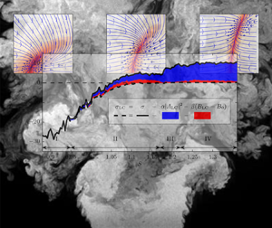
Figure 12 shows the estimated amplification rate obtained from the calibration of the mean-field model. The graph gives the linear amplification rate similar to figure 9, and further details which mechanism in the model leads to the saturation at the limit cycle. The coloured areas indicate different contributions to the saturation of the amplification rate at the limit cycle as given in (4.3). Accordingly, the effective amplification rate at the limit cycle is given by

(4.6)\begin{equation} \sigma_{{\textit{LC}}} = \sigma - \alpha |A_{\textit{LC}}|^2 - \beta (B_{\textit{LC}}-B_0), \end{equation}

where the subscript LC refers to a specific amplitude at the limit cycle. The two contributions that lead to the reduction of the initial linear amplification rate $\sigma$ to the amplification rate at the limit cycle $\sigma _{{\textit{LC}}}$ are shown. The differences due to the direct saturation $\alpha |A_{\textit{LC}}|^2$ and the delayed saturation $\beta (B_{\textit{LC}}-B_0)$ are indicated on the graph. In contrast to the estimates from the amplitude equation (figure 10), which showed a bifurcation at $S=1.1$, the mean-field model shows a bifurcation of the flow at $S=1.05$. Figure 12 further shows that the delayed saturation is much more relevant in regime II. In regime IV, the main contribution comes from the direct saturation term in the model. For the larger swirl numbers, the two saturation mechanisms always add up to neutral stability at the limit cycle ($\sigma _{\textit{LC}}\approx 0$). Furthermore, the magnitude of the linear amplification rate $\sigma$ in regime II goes clearly above the zero line, in contrast to the previous estimation from the amplitude equation (figure 10). This is more consistent with the continuous increase of the limit-cycle amplitude observed in figure 9.

Figure 12.

Estimated model parameters from pressure measurements using the mean-field model. The coloured areas indicate different contributions to the saturation of the amplification rate in (4.6). The arrows and vertical dotted lines indicate different regimes in the swirl-number range.

The agreement of the observed and modelled drift coefficients, as well as the consistent description of the flow physics, suggest a more reliable description of the bifurcation by the mean-field model than the amplitude equation. Especially at the bifurcation point, the secondary dynamics from the shift-mode contribute significantly to the dynamics of the oscillatory mode, which causes the deviation from the simpler approach based on the amplitude equation.

4.3. Insights from the description of the flow by the mean-field model

The parameters estimated from the 2-D mean-field model (4.3) and (4.4) allow an accurate description of the dominant flow dynamics consistent with the 1-D amplitude equation (3.5). The 2-D model, however, differs in two main points: (i) the identified bifurcation point and (ii) the growth rates for swirl numbers closely beyond the bifurcation point. The 2-D model reveals that the interaction of the shift-mode and the oscillatory mode in this regime is of great importance, which is not covered by the 1-D model. Hence, neglecting the shift-mode and describing the system solely based on the amplitude makes it a non-Markovian process, which cannot be covered by the proposed Langevin equation. The unresolved dynamics between the shift-mode and oscillatory mode causes the additive noise to be correlated with the dynamics, which violates the basic assumptions.

The pressure-sensor-based estimation of the mode amplitude does not provide an exact reproduction of the helical-mode amplitude as obtained from the PIV measurements. The pressure-based estimation is contaminated by the streamwise movement of the breakdown bubble position, which is connected to the shift-mode amplitude. This interaction is further investigated in Appendix B, where it is shown that a part of the amplitude variations might be attributed to a modulation by the shift-mode. However, it is not entirely clear if this results from a delay between the local pressure-based estimate and the global determination from PIV, or if it is simply an amplitude modulation. Consequently, it is possible that the delayed saturation in the model is caused not by flow dynamics but by the measurement principle. Nevertheless, incorporating this additional influence in the model allows one to describe the correlated dynamics in the data and brings the model in line with the correlations of the measured dynamics.

The results from the calibration of the mean-field model provide a deeper understanding of the dynamics governing the swirling flow. The corresponding properties of the flow model are summarised in figure 13(a). Two distinct flow states can be derived from the model: (i) the base flow, which constitutes the quasi-stationary state of the flow before the onset of the instability; and (ii) the mean flow, which is the mean velocity field corresponding to the instability oscillating at the limit cycle. The base flow is a state that is rarely reached in unstable conditions due to the unavoidable external perturbations from turbulence and instabilities. It can only be obtained artificially through active flow control or from transient investigations of the flow. The unique feature of the current approach is that one can make statements about the stationary base flow state, although one considers only fluctuations around the mean flow state.

Figure 13.

(a) Reduced schematic of one of the plots from figure 11, where the mean-field paraboloid is indicated as the dashed line. The base flow is indicated by $B_0$ and the mean flow (limit cycle) by $B_{\textit{LC}}$. (b) Simulated time series of the mean-field model for $S=1.12$, where the line is coloured by the simulation time (from blue to red). The time series starts at $B=B_{\textit{LC}}$ and $A=0$, the unperturbed mean flow.

More generally, the better understanding of the interaction between hydrodynamic instabilities and the mean flow helps to link the experimental observations and numerical results from mean-flow stability analysis beyond the comparison of mode shapes. The quantitative assessment of amplification rates and mean-flow corrections from measurements allows a direct comparison of both approaches. Moreover, the distinction between deterministic and stochastic parts and their contribution to the flow dynamics enriches the picture of hydrodynamic instabilities in turbulent flows and helps to interpret the amplification rates obtained from mean-flow stability analysis. The effective limit-cycle amplification rate (see figure 12) should be directly comparable to the amplification rate of a corresponding mean-flow stability analysis.

The simulation of a time series shown in figure 13(b), starting from the mean flow with no oscillations, further illustrates the essence of the mean-field model. Before the oscillations grow significantly, the flow rapidly shifts towards the base flow and then grows in amplitude along the mean-field paraboloid. This behaviour is consistently observed for simulations of a cylinder wake (Noack et al. Reference Noack, Afanasiev, Morzyński, Tadmor and Thiele2003; Brunton et al. Reference Brunton, Proctor and Kutz2016), where the mean-field paraboloid is also identified as an inertial/slow manifold. The drift in state space (figure 13a) clearly shows that the mean-field paraboloid constitutes an attracting, slow manifold for the swirling jet. This knowledge of the mean-field model helps to understand the transient and intermittent dynamics of the swirling jet.