1. Introduction
A gravity current is a buoyancy-driven flow in which predominantly horizontal pressure gradient forces cause fluid of one density to flow under or over fluid of another density. Gravity currents occur in nature as sea breezes, oceanic overflows, river flows and avalanches, and also appear in many engineering applications (Simpson Reference Simpson1997).
There have been many laboratory studies of lock–release gravity currents propagating on flat surfaces, including those by Keulegan (Reference Keulegan1957), Huppert & Simpson (Reference Huppert and Simpson1980), Simpson (Reference Simpson1982), Rottman & Simpson (Reference Rottman and Simpson1983) and Shin, Dalziel & Linden (Reference Shin, Dalziel and Linden2004). The three phases of gravity current flow for a high-Reynolds-number lock–release gravity current on a horizontal surface are described by Huppert & Simpson (Reference Huppert and Simpson1980). In the first phase, shortly after the lock is released, the gravity current flows steadily during what is called the constant-speed (or slumping) phase. For an energy-conserving gravity current produced by full-depth lock–release in a rectangular channel of depth
 $H$
, Benjamin (Reference Benjamin1968) predicted the height and speed of the current to be
 $h=H/2$
and
 $U_{0}=\sqrt{g^{\prime }H}/2$
, respectively, in which
 $g^{\prime }$
is the reduced gravity based on the density difference between the current and ambient fluid. This work was verified experimentally by Shin et al. (Reference Shin, Dalziel and Linden2004), who extended the theory for energy-conserving gravity currents released from partial-depth locks. In the second phase, after propagating 6–10 lock lengths the speed of the current front decreases, the front position changing in time according to
 $X\sim t^{2/3}$
(Rottman & Simpson Reference Rottman and Simpson1983). This is called the inertial (self-similar) phase. Finally, the current enters the third, so-called viscous phase, in which the front advances at a still slower rate due to the effects of viscosity.
Gravity currents flowing down shallow to moderate slopes were examined in experiments with a constant volume flux at the source (Britter & Linden Reference Britter and Linden1980) and in lock–release (constant volume source) experiments with corresponding simulations (Birman et al.
Reference Birman, Battandier, Meiburg and Linden2007). They found broadly similar results, namely that downslope gravity currents are quasi-steady and that the speed of the current varies moderately with the slope angle. In particular, for downslope lock–release gravity currents, Birman et al. (Reference Birman, Battandier, Meiburg and Linden2007) found that the front speed relative to the speed of horizontal currents is larger by approximately 10 % for downward slopes of
 $s\simeq \tan 10^{\circ }$
and is approximately 20 % faster when propagating down a slope of
 $s\simeq \tan 40^{\circ }$
, for which the current speed was found to be fastest.
The evolution of gravity currents flowing up a slope has been examined numerically by Safrai & Tkachenko (Reference Safrai and Tkachenko2009). Though focusing upon turbulent entrainment processes, they did observe that the current decelerated while moving upslope, with greater deceleration on larger slopes. Similar behaviour was observed by Ottolenghi et al. (Reference Ottolenghi, Adduce, Inghilesi, Roman and Armenio2015), who examined a combination of large-eddy simulations and laboratory experiments of upslope currents. Marleau, Flynn & Sutherland (Reference Marleau, Flynn and Sutherland2014) performed laboratory experiments examining the approach towards and propagation upon a rising slope of full- and partial-depth lock–release gravity currents. Consistent with the predictions of a Wentzel–Kramers–Brillouin (WKB) like theory, they observed nearly constant deceleration along the uniform slope,
 $s$
, with a horizontal component of acceleration
 $a_{x}=-0.112g^{\prime }s(D_{0}/H_{0})(2-D_{0}/H_{0})$
, in which
 $D_{0}$
is the depth of the lock fluid and
 $H_{0}$
is the ambient fluid depth at the start of the slope. In particular, for full-depth lock–release experiments (
 $D_{0}=H_{0}$
), they found
 $a_{x}=-0.112g^{\prime }s$
.
Monaghan, Mériaux & Huppert (Reference Monaghan, Mériaux and Huppert2009) used a combination of a theoretical box model and laboratory experiments to show that lock–release gravity currents in a horizontal V-shaped valley exhibited very similar behaviour in the constant-speed and inertial phase to lock–release gravity currents in a rectangular channel. In the inertial phase, however, they predicted that the front location changed in time according to
 $X\sim t^{4/5}$
.
Marino & Thomas (Reference Marino and Thomas2009) followed the approach of Benjamin (Reference Benjamin1968) to formulate a prediction for the steady speed of a gravity current propagating in a horizontal channel having cross-sectional width that changed as a power law with height,
 $z$
, according to
 $bz^{{\it\alpha}}$
for constants
 $b$
and
 ${\it\alpha}$
. The result was generalized further by Ungarish (Reference Ungarish2013) and Zemach & Ungarish (Reference Zemach and Ungarish2013), who predicted the steady speed in horizontal channels of arbitrarily varying width with height. Using a hydrostatic shallow-water formulation, they solved the equations for lock–release gravity currents in various horizontal channel geometries, including a V-shaped valley. The simulated front position over time agreed well with the experiments by Monaghan et al. (Reference Monaghan, Mériaux and Huppert2009) and Ungarish, Mériaux & Kurz-Besson (Reference Ungarish, Mériaux and Kurz-Besson2014) in both the constant-speed and inertial phases. Other studies of gravity currents in V-shaped valleys have explored the effects of viscosity (Takagi & Huppert Reference Takagi and Huppert2007) and rotation (Darelius Reference Darelius2008; Cuthbertson et al.
Reference Cuthbertson, Lundberg, Davies and Laanearu2014).
There have been relatively few laboratory studies of high-Reynolds-number gravity currents in more complex geometries, and what little has been done has mainly been limited to flow over obstacles (Rottman et al. Reference Rottman, Simpson, Hunt and Britter1985; Lane-Serff, Beal & Hadfield Reference Lane-Serff, Beal and Hadfield1995) and to surface currents above a uniform slope (Sutherland, Polet & Campbell Reference Sutherland, Polet and Campbell2013).
The novelty of the present study lies in investigating a dense full-depth lock–release gravity current propagating both upslope and within a V-shaped valley. A combination of theory, numerical simulations and laboratory experiments is used to understand the dynamics of this flow. Besides its fundamental interest, this idealized problem constitutes the first step in understanding the more complex dynamics of a sea breeze as it moves uphill and through valleys in coastal regions.
Section 2 reviews recent theories for gravity currents in channels of arbitrarily varying width with height and specifically considers the steady speed of an energy-conserving gravity current in a horizontal V-shaped valley. Separately, a theoretical model predicting the deceleration of flow up a slope is reviewed and extended for upslope V-shaped valleys. Section 3 presents the set-up, analysis methods and results of laboratory experiments of gravity currents that propagate horizontally and upslope in rectangular channels and V-shaped valleys. Section 4 describes the hydrostatic model that is used to simulate the experiments using the same configuration and comparable parameter ranges. The simulated front speed and deceleration are compared with theory and experiments and the structure of the simulated current is compared with experiments. Thus we assess the ability of a hydrostatic code to capture the evolution of a gravity current in this somewhat complex geometry. Section 5 summarizes the results.
2. Theory
2.1. Steady speed of a current in a horizontal V-shaped valley
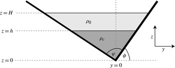
We consider a gravity current of maximum height
 $h$
flowing steadily in an ambient fluid of maximum depth
 $H$
propagating in a horizontal V-shaped valley having spread
 ${\it\varphi}$
and spanwise tilt
 ${\it\phi}$
, as illustrated in figure 1. The current is assumed to have uniform density
 ${\it\rho}_{c}$
and the ambient fluid has density
 ${\it\rho}_{0}$
, so that the reduced gravity is
 $g^{\prime }=g({\it\rho}_{c}-{\it\rho}_{0})/{\it\rho}_{c}$
.
Schematic spanwise cross-section downstream of a gravity current head as it flows steadily in a horizontal V-shaped valley with spread
 ${\it\varphi}$
and tilt
 ${\it\phi}$
. For the purposes of theory, the interface between the current and ambient fluid downstream of the current head is assumed to be horizontal with depth
 $h$
above the deepest part of the channel.

Following the approach of Benjamin (Reference Benjamin1968), Marino & Thomas (Reference Marino and Thomas2009) predicted the steady speed of a gravity current propagating in a lengthwise uniform domain whose spanwise width increased with height
 $z$
according to
 $W(z)=bz^{{\it\alpha}}$
. This description included the special cases of a rectangular channel (
 ${\it\alpha}=0$
) and a V-shaped valley (
 ${\it\alpha}=1$
). From conservation of momentum and mass, they derived an expression for the steady speed
 $U_{0}$
of the gravity current as a function of the relative downstream height,
 $h/H$
:
 $$\begin{eqnarray}U_{0}^{2}=2\left(\frac{1-\left(\displaystyle \frac{h}{H}\right)^{1+{\it\alpha}}}{1+\left(\displaystyle \frac{h}{H}\right)^{1+{\it\alpha}}}\right)\left(1-\frac{1}{2+{\it\alpha}}\left(\frac{h}{H}\right)^{1+{\it\alpha}}\right)g^{\prime }h.\end{eqnarray}$$
In the case
 ${\it\alpha}=0$
, this gives the well-known prediction (Benjamin Reference Benjamin1968; Klemp, Rotunno & Skamarock Reference Klemp, Rotunno and Skamarock1994) for the speed of gravity currents in a rectangular channel.
In the case of a V-shaped valley, for which
 ${\it\alpha}=1$
, the speed of a gravity current is predicted to be
 $$\begin{eqnarray}U_{0}^{2}=2\left(\frac{1-\left(\displaystyle \frac{h}{H}\right)^{2}}{1+\left(\displaystyle \frac{h}{H}\right)^{2}}\right)\left(1-\frac{1}{3}\!\left(\frac{h}{H}\right)^{2}\right)g^{\prime }h.\end{eqnarray}$$
The above expression applies for valleys of arbitrary tilt and spread.
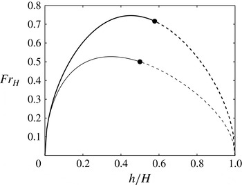
The predicted relative speeds of a gravity current in a rectangular channel and a V-shaped valley given as a function of the relative current depth are plotted in figure 2. Explicitly, the speed is cast in terms of a Froude number based upon the maximum ambient fluid depth,
 $$\begin{eqnarray}\mathit{Fr}_{H}\equiv U_{0}/\sqrt{g^{\prime }H},\end{eqnarray}$$
and the maximum current depth is given relative to the maximum ambient fluid depth. Here we have chosen to cast the Froude number in terms of
 $H$
rather than the maximum gravity current height,
 $h$
, because the latter is difficult to measure in laboratory experiments.
Dependence of Froude number,
 $\mathit{Fr}_{H}\equiv U_{0}/\sqrt{g^{\prime }H}$
, on the relative downstream height of the gravity current propagating horizontally in a rectangular channel (thin line) and, from (2.2), in a V-shaped valley (thick line). Solid circles indicate values for energy-conserving gravity currents and dashed lines denote unrealizable values that require external energy to maintain the flow. Note that for a current in a V-shaped valley,
 $\mathit{Fr}_{H}$
is independent of the valley spread and tilt,
 ${\it\varphi}$
and
 ${\it\phi}$
, respectively.

Assuming that, in addition to mass and momentum, energy is conserved, then the relative height is constrained to be (Marino & Thomas Reference Marino and Thomas2009)
 $$\begin{eqnarray}\frac{h}{H}=\left(\frac{1}{2+{\it\alpha}}\right)^{1/(1+{\it\alpha})},\end{eqnarray}$$
and the steady speed is
 $$\begin{eqnarray}U_{0}=\sqrt{2}\left(\frac{1+{\it\alpha}}{2+{\it\alpha}}\right)\sqrt{g^{\prime }h}.\end{eqnarray}$$
Specifically, in the case of the rectangular channel, we have the Benjamin (Reference Benjamin1968) results that
 $$\begin{eqnarray}h=H/2\end{eqnarray}$$
and
 $$\begin{eqnarray}U_{0}=(g^{\prime }H)^{1/2}/2.\end{eqnarray}$$
Hence
 $\mathit{Fr}_{H}=1/2$
, which is moderately smaller than the maximum value of
 $\simeq 0.527$
occurring for
 $h/H\simeq 0.347$
. The experiments of Shin et al. (Reference Shin, Dalziel and Linden2004) confirmed that full-depth lock–release gravity currents indeed occupy half the depth of the ambient fluid and propagate in steady state with a Froude number approximately 5 % smaller than the energy-conserving value of
 $1/2$
. The discrepancy is attributed to energy loss resulting from turbulence between the current head and ambient fluid.
For a V-shaped valley, the height of an energy-conserving gravity current is predicted to be
 $$\begin{eqnarray}h=H/\sqrt{3}\approx 0.577H\end{eqnarray}$$
and its speed is
 $$\begin{eqnarray}U_{0}=\frac{2\sqrt{2}}{3\sqrt[4]{3}}\sqrt{g^{\prime }H}\approx 0.716\sqrt{g^{\prime }H}.\end{eqnarray}$$
Consistent with observations of gravity currents in horizontal rectangular channels, we expect that (2.8) and (2.9) should predict the height and speed of an energy-conserving gravity current resulting from a full-depth lock–release in a horizontal V-shaped valley with any spread or tilt. Like the rectangular channel case, the energy-conserving value of
 $\mathit{Fr}_{H}$
for a V-shaped valley is moderately smaller than its maximum value of
 $\simeq 0.746$
, which occurs for
 $h/H=0.452$
.
The fact that the speed of an energy-conserving gravity current in a V-shaped valley is larger than its counterpart in a rectangular channel can be understood because its relative height
 $h/H$
is approximately 15 % larger and so the current is driven by a larger horizontal pressure gradient. In a valley, the cross-sectional area of the current goes as the square of the height of the current. Therefore, for a current of the same cross-sectional area as the rectangular channel, a higher relative height is necessary. Owing to conservation of energy and momentum, the cross-sectional area of the current is only one-third of the total cross-sectional area of the V-shaped valley. The overlying ambient return flow takes up more area and is therefore slower. In the case of a rectangular channel, for which the cross-sectional areas of the current and ambient fluid are equal, the velocity of the current is equal to the velocity of the return flow.
2.2. Upslope deceleration
In our study of currents propagating in V-shaped valleys, we consider currents that propagate horizontally and upslope, as illustrated in figure 3. Although no rigorous theory exists for currents that propagate upslope in V-shaped valleys, we can extend the WKB like theory of Marleau et al. (Reference Marleau, Flynn and Sutherland2014), derived for upslope currents in a rectangular channel, to predict the deceleration of a current flowing up a valley. The theory assumes a constant Froude number,
 $\mathit{Fr}_{H}$
, so that the speed of the current at a given location
 $x$
depended only on the height
 $H(x)$
of the ambient fluid at the front of the current through
 $$\begin{eqnarray}U=\mathit{Fr}_{H}\sqrt{g^{\prime }H(x)}.\end{eqnarray}$$
The assumption of constant
 $\mathit{Fr}_{H}$
is equivalent to assuming that the ratio of local current to ambient fluid depth is constant (see (2.1)).
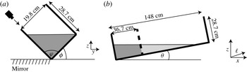
Schematic of the initial configuration of the laboratory experiments, showing (a) a spanwise cross-section across the lock and (b) a lengthwise cross-section along the deepest part of the valley, with the gate indicated by the thick dashed line. In panel (a) the position of the camera is shown to be looking down the side of the tank to produce a top view of the current through the ambient fluid and a side view of the current through light reflected from the mirror (hashed markings). The bottom lengthwise slope is given in terms of the rise angle
 ${\it\theta}$
by
 $s=\tan {\it\theta}$
. The along-slope coordinate system is represented by
 $\ell$
and the projection of this coordinate onto the horizontal is
 $x=\ell \cos {\it\theta}$
.

Setting the front speed
 $U=\text{d}x/\text{d}t$
gives a differential equation that can be solved to find the front position
 $x\equiv X(t)$
. In particular, for a uniform slope
 $s$
and an initial front speed
 $U_{0}=\mathit{Fr}_{H}\sqrt{g^{\prime }H_{0}}$
at
 $X=X_{0}$
, where
 $H(X_{0})=H_{0}$
, the front position is predicted to change in time according to
 $$\begin{eqnarray}X=X_{0}+U_{0}t-\frac{U_{0}^{2}s}{4H_{0}}t^{2}.\end{eqnarray}$$
Therefore, the along-slope acceleration is predicted to be constant and negative, with horizontal component
 $$\begin{eqnarray}A_{x}=-\frac{1}{2}\frac{U_{0}^{2}}{H_{0}}s=-\frac{1}{2}\mathit{Fr}_{H}^{2}g^{\prime }s.\end{eqnarray}$$
In full-depth lock–release experiments in a lengthwise sloping tank, the current is expected to accelerate rapidly from rest to a speed
 $U_{0}$
over a short distance from the gate after it is extracted. If the slope of the tank is sufficiently small, this speed should be comparable to the energy-conserving speeds of gravity currents in a horizontal channel. Thus in a rectangular channel, for which
 $U_{0}$
is given by (2.7), the consequent gradual deceleration of the current as it runs upslope is predicted by
 $$\begin{eqnarray}A_{x}=-g^{\prime }s/8=-0.125g^{\prime }s.\end{eqnarray}$$
This prediction is close to the deceleration measured for gravity currents in a rectangular channel incident upon a slope (Marleau et al. Reference Marleau, Flynn and Sutherland2014).
Because the information about the cross-channel geometry in (2.12) is captured by the Froude number, we anticipate that the deceleration of a gravity current in an upsloping V-shaped valley should be given by (2.12) in which
 $U_{0}$
is given by (2.9). Explicitly,
 $$\begin{eqnarray}A_{x}=-\frac{4}{9\sqrt{3}}\,g^{\prime }s\simeq -0.257g^{\prime }s.\end{eqnarray}$$
These predictions are compared with the results of laboratory experiments and numerical simulations in the next two sections.
3. Laboratory experiments
3.1. Laboratory set-up
The experimental set-up is illustrated in figure 3. The rectangular tank had length
 $148~\text{cm}$
, width
 $19.8~\text{cm}$
and height
 $28.7~\text{cm}$
. The sides of the tank were at right angles to each other, meaning that the valley spread was
 ${\it\varphi}=90^{\circ }$
in all experiments.
Blocks under the end of the table and a rail along the edge of the tank allowed the slope angle
 ${\it\theta}=\tan ^{-1}(s)$
, in which
 $s$
is the slope, and tilt
 ${\it\phi}$
to be varied independently with
 ${\it\theta}=0^{\circ },1^{\circ },2^{\circ },\dots ,7^{\circ },8^{\circ }$
and
 ${\it\phi}=0^{\circ },15^{\circ },30^{\circ },45^{\circ }$
. Here we compare upslope flows in a V-shaped valley (
 ${\it\theta}>0^{\circ },{\it\phi}>0^{\circ }$
) to horizontal flows in a V-shaped valley (
 ${\it\theta}=0^{\circ },~{\it\phi}>0^{\circ }$
) and to upslope flows in a rectangular channel (
 ${\it\theta}>0^{\circ },~{\it\phi}=0^{\circ }$
).
A gate of thickness
 $1~\text{cm}$
was positioned
 $36.7~\text{cm}$
from the left-hand end of the tank with a silicone seal to prevent water in the lock to the left of the gate from leaking into the ambient fluid to the right of the gate until the gate was extracted. A rail of height
 $0.5~\text{cm}$
held the gate perpendicular to the sides of the tank. Because the lock length was one-quarter of the total length of the tank, the current released from the lock in horizontal tank experiments (
 ${\it\theta}=0^{\circ }$
) was expected to propagate at constant speed to the end of the tank before entering the self-similar regime (Rottman & Simpson Reference Rottman and Simpson1983).
Salt was added to the water in the lock to increase its density, and after thorough mixing it was dyed with food colouring in order to visualize the advance of the gravity current after release from the lock. The density of the fluid on each side of the lock was then measured with an accuracy of
 $5\times 10^{-5}~\text{g}~\text{cm}^{-3}$
using an Anton Paar DMA 58 densitometer. In all the experiments, the resulting reduced gravity
 $g^{\prime }$
was approximately
 $6~\text{cm}~\text{s}^{-2}$
.
The tank was filled with water to a depth that varied depending upon the tilt angle
 ${\it\phi}$
in order to ensure that the fluid in the tank was bounded laterally only by the two outward sloping sidewalls of the tank (figure 3
a). The greatest depth of fluid at the gate,
 $H_{0}$
, was
 $15.5~\text{cm}$
for a rectangular channel (
 ${\it\phi}=0^{\circ }$
),
 $5~\text{cm}$
for
 ${\it\phi}=15^{\circ }$
,
 $9.9~\text{cm}$
for
 ${\it\phi}=30^{\circ }$
and
 $10~\text{cm}$
for
 ${\it\phi}=45^{\circ }$
. These lock depths caused the end of the tank to be dry in some of the valley experiments where the rise angle was moderately large (
 ${\it\theta}>3^{\circ }$
).
For flow in a rectangular channel, the typical Reynolds number was
 $\mathit{Re}=H_{0}U_{0}/{\it\nu}\approx 8000$
based on the ambient fluid height and the anticipated energy-conserving speed given by (2.7). In the V-shaped valley experiments, for which
 $U_{0}$
is estimated by (2.9), the value of
 $H_{0}$
was smaller, resulting in lower-Reynolds-number flows. Explicitly,
 $\mathit{Re}\sim 5000$
for
 ${\it\phi}=45^{\circ }$
and
 ${\it\phi}=30^{\circ }$
, and
 $\mathit{Re}\sim 2500$
for
 ${\it\phi}=15^{\circ }$
. In all cases, the Reynolds number is sufficiently large that viscosity should play a negligible role in the evolution of the current close to the gate and during the initial stage of deceleration in upsloping experiments. However, viscosity is expected to play a role at the sides of the valley where the fluid is shallow and at late times in experiments with moderately large rise angles, as the current slows to a halt where the surface touches the tank bottom.
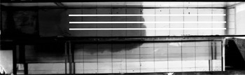
A movable Hitachi KPF 100 camera was positioned above the tank, angled so that it looked along the tank wall, as illustrated in figure 3(a). In rectangular channel experiments, a mirror was placed at 45° to the horizontal so that the camera would simultaneously record a side view of the current, as shown in figure 4. In V-shaped valley experiments, the mirror was placed flat on the table supporting the tank, as illustrated in figure 3(a). In this case the view from the mirror compared with the view through the open end of the tank enabled us to evaluate the symmetry of the gravity current.
Snapshot taken from an experiment of a gravity current propagating along a horizontal rectangular channel in an ambient fluid of depth
 $H_{0}=15.5~\text{cm}$
and with reduced gravity
 $g^{\prime }=6.57~\text{cm}~\text{s}^{-2}$
. The upper part of the image shows a top view looking through the surface of the (clear) ambient fluid to the dyed current whose front is situated approximately 50 cm to the right of the gate. The bottom part of the image shows the side view of the current visualized by a mirror tilted at 45° from the horizontal along the length of the tank. The three white lines indicate where along-tank slices were taken to construct time-series images of the rightward-advancing current front.

When the gate was extracted, the dyed lock fluid flowed along the bottom of the tank as a gravity current. A grid on the bottom of the tank was used to locate the position of the head of the current as it propagated along the tank. The lines of the grid were spaced every
 $5~\text{cm}$
in the spanwise (
 $y$
) direction and every
 $10~\text{cm}$
in the along-slope (
 $\ell$
) direction.
Movies were recorded at a rate of 10 fps, and recording continued until the current front reached the end of the tank or until the front became stationary in upsloping cases where the free surface intersected the tank bottom.
3.2. Analysis
Time series of the front position were constructed from movies of the experiments. Explicitly, slices from each frame of a movie were extracted along lines approximately parallel to the long side of the tank. In rectangular channel experiments, three slices were taken along lines spaced by
 $5~\text{cm}$
across the tank, as illustrated by the white lines in figure 4. In V-shaped valley experiments, the slices were taken a few pixels apart against the near tank wall.
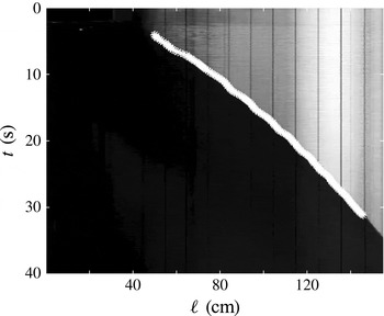
A threshold in brightness intensity was used to define which fluid belonged to the current. The position of the front was then determined from the location of the contour with this intensity in each time-series image, as illustrated in figure 5.
Time series taken from an experiment of a gravity current propagating upslope in a rectangular channel with
 $H_{0}=15.5~\text{cm},g^{\prime }=6.49~\text{cm}~\text{s}^{-2}$
and
 ${\it\theta}=6.2^{\circ }$
(
 $s\simeq 0.11$
). The closely spaced overlapping white stars indicate points selected to determine the along-slope front position,
 $\ell$
, versus time,
 $t$
.

When the gate was removed, the fluid adjusted for a few seconds before the gravity current formed. For this reason, data from the first two seconds of each experiment were discarded. Data taken within 10 cm of the right-hand side of the tank were also discarded because surface waves reflecting off the end of the tank tended to cause oscillations of the front in this region, particularly for currents propagating upslope. In V-shaped valley experiments, the images of the current were obstructed by clamps that tilted the tank at an angle. Data points in these locations were also discarded.
Anticipating that the upslope-propagating front should decelerate according to (2.11), we found the best-fitting quadratic to the measured along-slope front position in the form
 $\ell =\ell _{0}+u_{\ell }t+(a_{\ell }t^{2})/2$
. The coefficients were used to find the horizontal component of the initial along-slope front speed
 $u_{0}=u_{\ell }\cos {\it\theta}$
and the horizontal component of the front acceleration
 $a_{x}=a_{\ell }\cos {\it\theta}$
. These results were compared with the predicted speed
 $U_{0}$
given by (2.7) and (2.9) and the acceleration
 $A_{x}$
given by (2.12).
This procedure was followed for each of the time series constructed from multiple slices along the tank. The mean and standard deviation of the measured values of
 $u_{0}$
and
 $a_{x}$
were then computed. In experiments where turbulence and mixing were observed, there was more spread in the values of
 $u_{0}$
and
 $a_{x}$
, but the spread (and therefore the error) was also influenced by the camera angle. In the V-shaped valley experiments, the results underestimated the true velocity and acceleration if the lines used to construct the time series were not exactly parallel to the tank wall. This may be the cause of some of the spread in the results.
3.3. Results
The measured horizontal component of the along-slope initial speed
 $u_{0}$
non-dimensionalized by
 $\sqrt{g^{\prime }H_{0}}$
(i.e. the Froude number) is plotted against rise angle
 ${\it\theta}$
as solid symbols in figure 6. In the case of a horizontal rectangular channel (
 ${\it\theta}=0^{\circ }$
), the observed Froude number is nearly 10 % lower than the predicted value of
 $\mathit{Fr}_{H}=U_{0}/\sqrt{g^{\prime }H_{0}}=1/2$
, but the measured values are consistent with those reported by Shin et al. (Reference Shin, Dalziel and Linden2004). As in their work, we attribute the difference to energy loss resulting from viscous dissipation and mixing.
Initial relative front speed,
 $u_{0}/\sqrt{g^{\prime }H_{0}}$
, versus the rise angle,
 ${\it\theta}$
. The front speed is determined from (solid symbols) laboratory experiments (E) and (open symbols) numerical simulations (N) of gravity currents in (a) a rectangular channel and (b) a V-shaped valley. The horizontal grey line in each panel indicates the predicted Froude number,
 $\mathit{Fr}_{H}=U_{0}/\sqrt{g^{\prime }H_{0}}$
, for horizontal channels and V-shaped valleys. In panel (b) different symbols are drawn depending upon the tilt,
 ${\it\phi}$
, of the V-shaped valley, as indicated in the legend. Errors in the measurements taken from laboratory experiments are no larger than the size of the symbols themselves.

Consistent with (2.9), the measured Froude number was larger for flow in a horizontal V-shaped valley than for flow in a horizontal rectangular channel. However, only the symmetric case with tilt
 ${\it\phi}=45^{\circ }$
gave
 $\mathit{Fr}_{H}\approx 0.714$
, close to the theoretical value of
 $2\sqrt{2}/(3\sqrt[4]{3})\simeq 0.716$
. For
 ${\it\phi}=15^{\circ }$
,
 $\mathit{Fr}_{H}$
was 22.4 % smaller, and for
 ${\it\phi}=30^{\circ }$
,
 $\mathit{Fr}_{H}$
was 17.1 % smaller, than the theoretical prediction. The greater discrepancy in the case
 ${\it\phi}=15^{\circ }$
is probably because the lock depth and hence the Reynolds number is smaller, so that viscous dissipation plays a more significant role.
In rectangular channel experiments (solid squares in figure 6
a), there is little change in Froude number as the rise angle,
 ${\it\theta}$
, increases from 0° to 8°. All measured values are smaller than the energy-conserving prediction by between 4 and 15 %. This observation is consistent with the expectation that the slope should not influence the initial speed if the slope is sufficiently small. Likewise, in V-shaped valley experiments, we did not observe any significant change in the Froude number with rise angle
 ${\it\theta}=6^{\circ }$
in the case with the valley having tilt
 ${\it\phi}=30^{\circ }$
(solid right-pointing triangles in figure 6
b). However, in experiments with tilt angle
 ${\it\phi}=45^{\circ }$
(solid circles in figure 6
b), we found that the Froude number did decrease moderately as
 ${\it\theta}$
increased from 0° to 8°, there being a 22 % difference between the measured and energy-conserving values when
 ${\it\theta}=8^{\circ }$
. The small number of experiments at asymmetric tilt angles makes it hard to draw any firm conclusions about the effect of slope on front speed in asymmetric valleys.
This Froude-number dependence upon
 ${\it\theta}$
with
 ${\it\phi}=45^{\circ }$
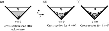
can be understood by considering the spanwise motion of fluid. After propagating some distance down the tank, the speed of the current front is highest in the middle of the valley where the along-tank pressure gradient is largest and where viscosity has the least influence over the depth of the current. The relatively faster flow leads to a depression in the interface between the current and ambient about
 $y=0$
, as illustrated in figure 7. Thus a spanwise flow develops in which dense fluid flows down the sides of the valley. A momentum deficit in the along-slope direction is transported from the edges of the dense current into the middle of the valley by the spanwise flow. This momentum deficit increases with increasing
 ${\it\theta}$
and is largest for tilt angle
 ${\it\phi}=45^{\circ }$
. Turbulence near the gravity current head should act to transport opposing momentum from the valley sides to the interior, slowing the front-propagation speed.
Schematic spanwise cross-section of the tilted tank showing the gravity current in grey and ambient flow in white (a) near the gate and (b) further downstream when propagating without a slope and (c) when flowing upslope.

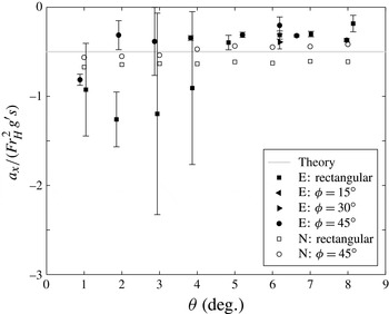
In figure 8 the measured horizontal component of the along-slope acceleration,
 $a_{x}$
, normalized by
 $\mathit{Fr}_{H}^{2}g^{\prime }s$
, is plotted versus the rise angle,
 ${\it\theta}$
. Here we set
 $\mathit{Fr}_{H}$
to be the Froude number for energy-conserving gravity currents: from (2.7),
 $\mathit{Fr}_{H}=1/2$
for currents in a rectangular channel; from (2.9),
 $\mathit{Fr}_{H}=2\sqrt{2}/(3\sqrt[4]{3})\approx 0.716$
for currents in a V-shaped valley. According to the rightmost expression in (2.12), the predicted horizontal component of (negative) acceleration,
 $A_{x}$
, when normalized by
 $\mathit{Fr}_{H}^{2}g^{\prime }s$
should be
 $-1/2$
for currents in rectangular channels and V-shaped valleys.
For small rise angles, gravity currents in a rectangular channel were found to decelerate faster than the theoretical prediction, but the error in these measurements was also significant, compounded by the fact that the normalized values are computed by taking the ratio of a small measured deceleration to a small slope
 $s$
. For rise angles
 ${\it\theta}\geqslant 5^{\circ }$
and for all the V-shaped valley experiments with
 ${\it\theta}\geqslant 2^{\circ }$
, we found that the measured deceleration of the current head was not as large as predicted, with typical values between 60 and 80 % of the predicted value.
Horizontal component of the (negative) relative acceleration,
 $a_{x}/(\mathit{Fr}_{H}^{2}g^{\prime }s)$
, versus the rise angle,
 ${\it\theta}$
. Here
 $\mathit{Fr}_{H}$
is the Froude number predicted for energy-conserving currents. Values are plotted for (solid symbols) laboratory experiments (E) and (open symbols) numerical simulations (N), with currents in a rectangular channel indicated by squares and currents in a V-shaped valley with tilt,
 ${\it\phi}$
, as indicated in the legend. The horizontal grey line is the (negative) relative acceleration predicted by theory. Errors in the measurements taken from laboratory experiments are indicated by vertical error bars.


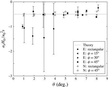
In figure 6 we showed that the measured relative speed differed from the predicted energy-conserving speed. With this consideration, in figure 9 we replot the measured acceleration data but normalize them using the middle expression of (2.12) in which we use the measured speed
 $u_{0}$
rather than the predicted energy-conserving speed
 $U_{0}$
. Again, theory predicts that the normalized acceleration,
 $a_{x}/({u_{0}}^{2}s/H_{0})$
, should be
 $-1/2$
. With this semi-empirical normalization, we find better agreement between experiments and theory, except in a small number of the experiments in the rectangular channel. These experiments have
 ${\it\theta}<5^{\circ }$
, and the change in value is small compared with the size of the error bars. Particularly for the V-shaped valley experiments, the measured normalized deceleration differs by less than 23 % from the predicted deceleration for all rise angles above 2°. Considering the approximations used to derive (2.12), this agreement suggests that the model captures the main physical processes at play.
4. Numerical simulations
4.1. Model set-up
Shallow-water theory, which assumes hydrostatic balance, has often been used to examine the evolution of gravity currents (Ungarish Reference Ungarish2009, Reference Ungarish2013). Here we examine the efficacy of a hydrostatic code in capturing the observed dynamics of upslope gravity currents in channels and valleys. Specifically, we used the hybrid coordinate ocean model (HYCOM) (Bleck Reference Bleck2002; Chassignet et al. Reference Chassignet, Smith, Halliwell and Bleck2003; Halliwell Reference Halliwell2004), a hydrostatic model commonly used to study ocean processes.
The code was set up in isopycnal coordinates to model the evolution of a hydrostatic two-layer fluid with no mixing allowed between the current and ambient fluid. The results are analogous to shallow-water theory. The domain was set to have the same size and shape as the tank used for the laboratory experiments. The horizontal resolution was
 $0.5~\text{cm}$
, except in the experiments with asymmetric valleys (
 ${\it\phi}\neq 45^{\circ }$
), in which case the horizontal resolution was set to
 $0.25~\text{cm}$
to accommodate for the smaller flow scales. Refinement of the grid had no effect on the recorded speed or acceleration of the gravity current. Because the code is hydrostatic, it does not resolve the short scales of the flow correctly, but the high resolution allows for a smaller viscosity, as described below, and for the topography to be well resolved.
The reduced gravity,
 $g^{\prime }$
, for all simulations was
 $4.79~\text{cm}~\text{s}^{-2}$
. While this differs from the experiments by around 20 %, all of the results presented below are non-dimensionalized by
 $g^{\prime }$
, and so the actual value of
 $g^{\prime }$
is irrelevant since the current is Boussinesq. It was verified that the non-dimensional speed and acceleration did not change if
 $g^{\prime }$
was varied by approximately 20 %. The depth of fluid at the lock gate,
 $H_{0}$
, varied with the tilt
 ${\it\phi}$
, as it did in the laboratory experiments. For numerical stability, but also to mimic unresolved turbulent processes, the viscosity was set to be 4–10 times larger than that of water. The corresponding Reynolds number, calculated using the predicted speed of the current and the ambient fluid depth at the gate, was
 $\mathit{Re}=800$
. This value is still sufficiently high that viscous effects are not expected to influence the speed and deceleration of the current at early times, although changes in viscosity do affect the shape of the current head.
The front was defined as the furthest downstream location at which the interface was more than
 $0.1~\text{cm}$
above the bottom of the model tank. Its position was computed every
 $0.2~\text{s}$
. As in the laboratory experiments, the best-fitting quadratic of the front position versus time was computed. From this, we measured the horizontal components of the initial speed,
 $u_{0}$
, and (negative) acceleration,
 $a_{x}$
.
4.2. Qualitative results
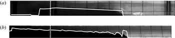
In figure 10 the interface between the current and ambient fluid computed from the hydrostatic code is compared with the structure observed in laboratory experiments. Consistent with shallow-water theory (Ungarish Reference Ungarish2009), the simulated current front is nearly vertical. For a horizontally propagating gravity current in a rectangular channel, the interface is nearly horizontal behind the front. However, the structure is more complex for a horizontally propagating gravity current in a V-shaped valley. Shortly behind the front, the simulated current height rapidly decreases and then gradually increases in height far in the lee of the current head. Being hydrostatic, the model is not expected to capture the structure of the front. The sharp front shown is typical of shallow-water theory for a gravity current. Indeed, in laboratory experiments the front of the gravity current is not vertical but slopes away from the bottom. Well behind the front, however, the hydrostatic code captures the near-horizontal interface between current and ambient fluid in a rectangular channel, and the gradually increasing current height with distance from the front for gravity currents in a V-shaped valley.
Side-view snapshots of gravity currents propagating horizontally in (a) a rectangular channel and (b) a V-shaped valley with tilt
 ${\it\phi}=45^{\circ }$
. The solid white line superimposed on both images shows the current height midway along the span of the tank taken from the numerical simulations at times when the computed front position is at the same location as the observed front position relative to the gate. The numerical simulations shown have
 $g^{\prime }=4.79~\text{cm}~\text{s}^{-2}$
, but changing the value of
 $g^{\prime }$
to its experimental value has very little effect on the shape of the head. The vertical dotted white line indicates the position of the gate.

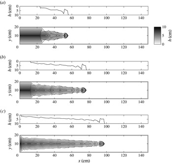
Figure 11 shows vertical cross-sections and contours of current height at three successive times for simulations of a horizontally propagating gravity current in a V-shaped valley with tilt
 ${\it\phi}=45^{\circ }$
. At each time, the head appears as a localized elevated region of along-tank length approximately
 $5~\text{cm}$
. The trailing tail gradually increases in depth with distance from the front, and superimposed on this sloping interface are wave-like structures that are found to travel backwards away from the front. The waves move in this direction because the front is supercritical, moving faster than the long-wave speed. There was no evidence of these waves in the laboratory experiments. We surmise that their manifestation was obstructed by turbulence, which is parametrized in the numerical simulations.
Structure of a horizontally propagating gravity current in a V-shaped valley with tilt
 ${\it\phi}=45^{\circ }$
as determined from simulations at times (a)
 $t=4$
s, (b)
 $t=8$
s and (c)
 $t=12$
s after release from the lock. In each pair, the upper panel shows the current height along a vertical cross-section at
 $y=0$
(the deepest part of the domain) and the lower panel shows contours of current thickness as a function of along-tank (
 $x$
) and across-tank (
 $y$
) coordinates. The grey scale (top right) determining the depth is the same for each lower panel.

4.3. Quantitative results
As well as showing the experimental measurements and theoretical predictions for the horizontal component of the initial speed
 $u_{0}$
, figure 6 plots the computed initial speed as open symbols. Unlike the laboratory experiments, the Froude number found in all simulations is moderately larger than the predicted Froude number for horizontally propagating energy-conserving currents. Explicitly, we found
 $u_{0}/\sqrt{g^{\prime }H_{0}}=0.53\pm 0.01$
for the rectangular channel and
 $u_{0}/\sqrt{g^{\prime }H_{0}}=0.745\pm 0.005$
for the V-shaped valley with
 ${\it\phi}=45^{\circ }$
. These values are consistent with the maximum Froude number occurring for dissipative currents with smaller relative downstream depth
 $h/H_{0}$
(see figure 2). In the rectangular channel, there is a maximum in the height of the gravity current immediately behind the front. At this maximum,
 $h/H\approx 0.35$
, consistent with the theoretical
 $h/H=0.347$
for maximum front velocity. In the simulations of the V-shaped valley, the height of the nose of the current is higher than the theory predicts, but the first maximum behind the nose has
 $h/H\approx 0.43$
, again consistent with a lower head height causing a faster speed (the theoretical head height for maximum speed is
 $h/H=0.452$
). Another difference from laboratory experiments is that in the simulations the initial speed had no significant dependence upon the rise angle even in the case of a V-shaped valley with tilt
 ${\it\phi}=45^{\circ }$
.
The horizontal component of acceleration,
 $a_{x}$
, determined from the simulations is plotted as open symbols in figures 8 and 9. As in the laboratory experiments, normalizing according to the middle expression in (2.12) and using the measured initial speed (i.e.
 $u_{0}^{2}s/H_{0}$
) leads to better agreement with the theoretical prediction than normalizing by the Froude number predicted for energy-conserving currents. Whether for simulations in a rectangular channel or a V-shaped valley, all values lie within 20 % of the predicted relative acceleration of
 $-1/2$
for rise angles between 1 and 8°. This suggests that non-hydrostatic processes do not play a significant role in determining the deceleration.
There is a small trend in the deceleration of the current in the V-shaped valley case: for high
 ${\it\theta}$
, the acceleration is less negative than theory predicts. The amount of fluid at the front is small, and so the speed of fluid further behind the front where
 $H$
is larger may be more relevant in determining the front speed.
5. Conclusions
Using a combination of theory, laboratory experiments and a hydrostatic numerical model, we have investigated the evolution of Boussinesq, full-depth lock–release gravity currents that propagate either horizontally or upslope in a rectangular channel or in a V-shaped valley.
In a horizontal V-shaped valley of arbitrary spread
 ${\it\varphi}$
and tilt
 ${\it\phi}$
, the Froude number of a steady energy-conserving gravity current was predicted to be
 $\mathit{Fr}_{H}=2\sqrt{2}/(3\sqrt[4]{3})\approx 0.716$
. Consistent with experiments of gravity currents in a rectangular channel, we found that experimental measurements of
 $\mathit{Fr}_{H}$
were up to 15 % smaller than this prediction. The simulated evolution of gravity currents using a hydrostatic code predicted moderately larger initial speeds. The shape of the simulated gravity current head also differed, exhibiting a sudden descent of the interface immediately behind the head near the middle of the cross-section.
In experiments of gravity currents running upslope, we found that the initial gravity current speed in a rectangular channel was not significantly affected by the rise angle of the tank. However, the initial gravity current speed in a V-shaped valley with tilt
 ${\it\phi}=45^{\circ }$
was found to decrease with increasing rise angle. In contrast, simulations of upslope gravity currents showed that the initial speed was independent of rise angle in all cases.
We attribute the discrepancies to turbulence, which appears to be enhanced in V-shaped valley experiments as a consequence of spanwise motions induced by lateral slumping of dense fluid down the sides of the valley. The turbulence slows the current due to enhanced dissipation and also due to enhanced transport of retrograde momentum across the span of the valley.
The WKB like theory of Marleau et al. (Reference Marleau, Flynn and Sutherland2014), which predicts the deceleration of upslope-propagating gravity currents in a rectangular channel, was adapted to the case of V-shaped valleys. In comparison with experiments and simulations, best agreement was found when the measured deceleration was normalized by the measured initial front speed,
 $u_{0}$
, rather than predicted speed,
 $U_{0}$
. Explicitly, for rectangular channels and V-shaped valleys, we found that the (negative) upslope acceleration was well represented by
 $$\begin{eqnarray}a_{x}\simeq -\frac{1}{2}\frac{{u_{0}}^{2}s}{H_{0}},\end{eqnarray}$$
for slopes at least as large as
 $s=\tan 8^{\circ }\simeq 0.14$
.
This work provides an important step towards understanding the more complex problem of a sea breeze propagating up valleys near coastal regions. In a coastal sea breeze,
 $H$
is not well defined, so partial-depth lock–release experiments may be instructive in exploring this phenomenon further. Future work might examine the effect of ambient stratification, meandering and rough topography and more realistic source conditions.
Acknowledgements
The authors gratefully acknowledge the National Science Foundation (grant OCE- 0824636) and the Office of Naval Research (grant N00014-09-1-0844) for their support of the 2013 WHOI Geophysical Fluid Dynamics Summer School, where much of the research presented in this paper was performed. We would also like to thank F. Gouillon and A. Bozec for their help in setting up and running HYCOM, and A. Jensen, who was very helpful in setting up the laboratory experiments.