1 Introduction
In the stimulation of oil and gas wells by hydraulic fracturing, the rheology of the fluid is the only thing that can be engineered (beside the value of the rate at which the fluid is injected). Large research efforts have thus led to the development of various fluid types over the years, essentially trying to maximize fracture opening and minimize particles settling (Economides & Nolte Reference Economides and Nolte2000; Barbati et al.
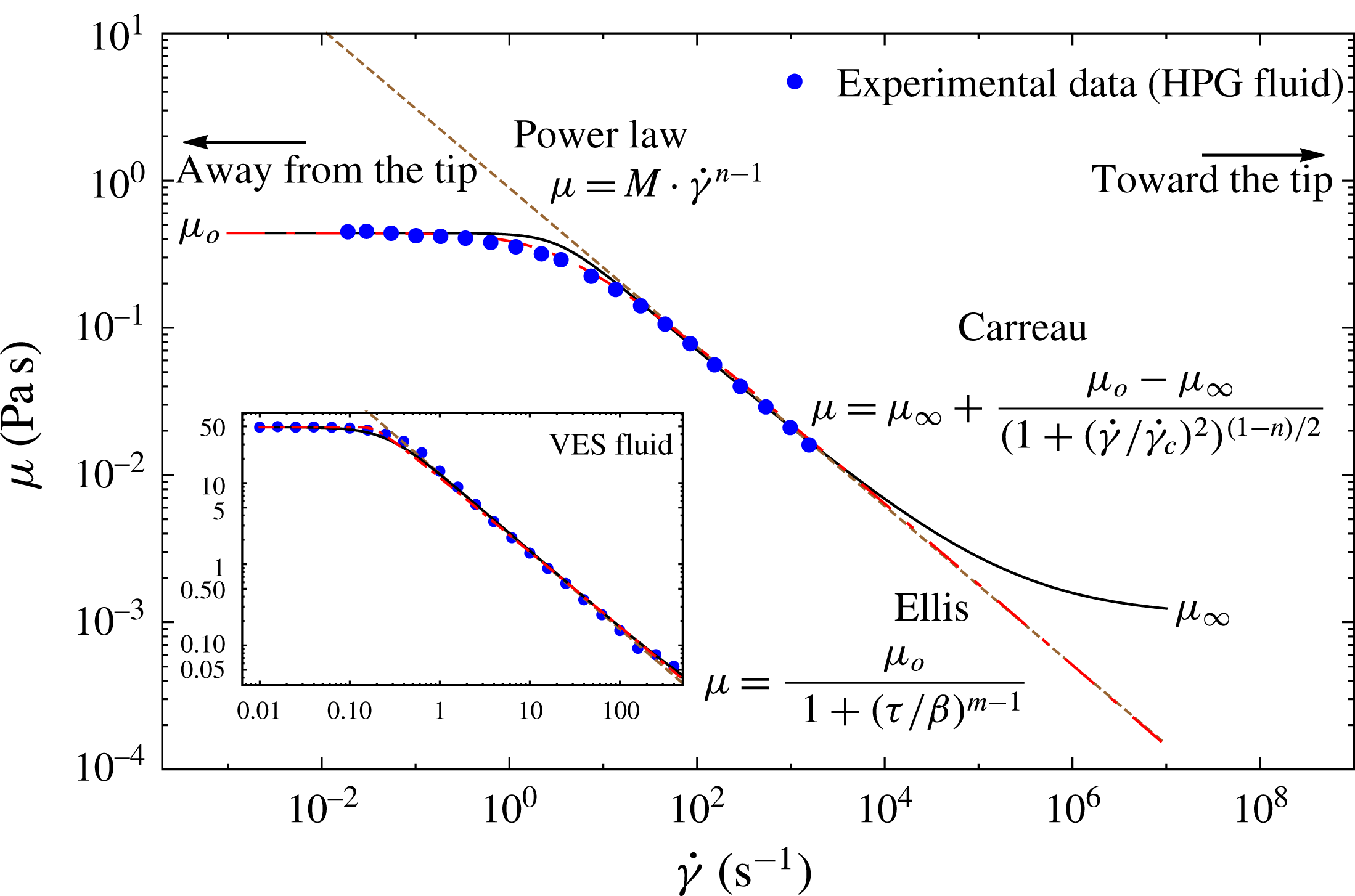
Reference Barbati, Desroches, Robisson and McKinley2016). Although other complex rheologies are sometimes encountered in practice (viscoelasticity, yield stress etc.), most of these engineered fluids exhibit a shear-thinning behaviour: their viscosity decreases as a function of the applied shear rate (see figure 1 for examples of the rheology of typical fracturing fluids). All these fluids exhibit a Newtonian plateau at low shear rate where their viscosity is maximum and starts to shear thin for value of shear rate larger than a critical value
 $\dot{\unicode[STIX]{x1D6FE}}_{c}$
. At very large shear rate, the viscosity tends to the Newtonian viscosity of the base solvent used (typically water). How such a complex rheological behaviour of the fluid impacts the actual propagation of a hydraulic fracture has been mostly investigated using a simple power-law model (e.g. Sousa, Carter & Ingraffea Reference Sousa, Carter and Ingraffea1993; Desroches et al.
Reference Desroches, Detournay, Lenoach, Papanastasiou, Pearson, Thiercelin and Cheng1994; Adachi & Detournay Reference Adachi and Detournay2002). The impact of the low and large shear rate plateau as well as the amplitude of shear thinning remain poorly understood. Similarly the effect of shear thinning on the extent of the fluid-less cavity at the fracture tip (fluid lag) observed for a Newtonian fluid (Garagash & Detournay Reference Garagash and Detournay2000) remains unknown.
Viscosity as function of shear rate for two fracturing fluids: Hydroxypropylguar (HPG – data taken from Guillot & Dunand Reference Guillot and Dunand1985) and in inset a viscoelastic surfactant (VES – data taken from Kefi et al. Reference Kefi, Lee, Pope, Sullivan, Nelson, Nunez Hernanez, Olsen, Parlar, Powers and Roy2004). These experimental data do not cover the large shear rate region where the viscosity typically tends toward the solvent viscosity (water in those cases) – see e.g. Pipe, Majmudar & McKinley (Reference Pipe, Majmudar and McKinley2008) for experimental data on Xanthan gum covering the complete range of shear rates. A number of rheological models can be used to reproduce these data over parts or all of the range of shear rates. We display here the best fit for the power-law (dashed brown line), Carreau (continuous black line) and Ellis (dot-dashed red line) rheological models. The corresponding best-fit parameters are listed in table 1 for these two fluids and the different models.

Rheological parameters of HPG and VES fluids (for a given temperature) for the power-law, Carreau and Ellis models corresponding to the experimental data of figure 1. Note that the majority of fracturing fluids have a power-law index
 $n$
between
 $0.1$
and
 $0.5$
.

The rheology of a shear-thinning fluid over the whole range of shear rates can be well reproduced by either the Cross (Reference Cross1965) or Carreau (Reference Carreau1972) constitutive models. We focus here on the Carreau rheology, but similar results would be obtained using the Cross model. Two others rheological models are often used for shear-thinning fluids: (i) the power-law model which captures only the shear-thinning part of rheological data (over-estimating viscosity at low shear rate, under-predicting at large shear rate) and (ii) the Ellis model (Brodkey Reference Brodkey1969) which reproduces the low shear rate Newtonian plateau as well as the power-law shear-thinning region but does not reproduce the large shear rate Newtonian limit. The differences between these models can be clearly seen in figure 1 while the corresponding rheological parameters are listed in table 1. In order to best fit the experimental data, the power-law index may be adjusted independently from the Carreau index (see examples in Myers Reference Myers2005; Sochi Reference Sochi2015). However, in the interest of comparison and simplification, we will consider that the power-law index is equal to the Carreau shear-thinning index. The power-law consistency
 $M$
(dimensions
 $\text{Pa}~\text{s}^{n}$
) can thus be expressed directly from the rheological parameters of the Carreau model:
 $$\begin{eqnarray}M=\frac{\unicode[STIX]{x1D707}_{o}+\unicode[STIX]{x1D707}_{\infty }}{2\dot{\unicode[STIX]{x1D6FE}_{c}}^{n-1}\left(\sqrt{2^{-2/(n-1)}-1}\right)^{n-1}},\end{eqnarray}$$
where
 $\unicode[STIX]{x1D707}_{o}$
,
 $\unicode[STIX]{x1D707}_{\infty }$
are the viscosity at low and high shear rates respectively and
 $\dot{\unicode[STIX]{x1D6FE}}_{c}$
is the critical shear rate at which the fluid starts to shear thin in the Carreau model.
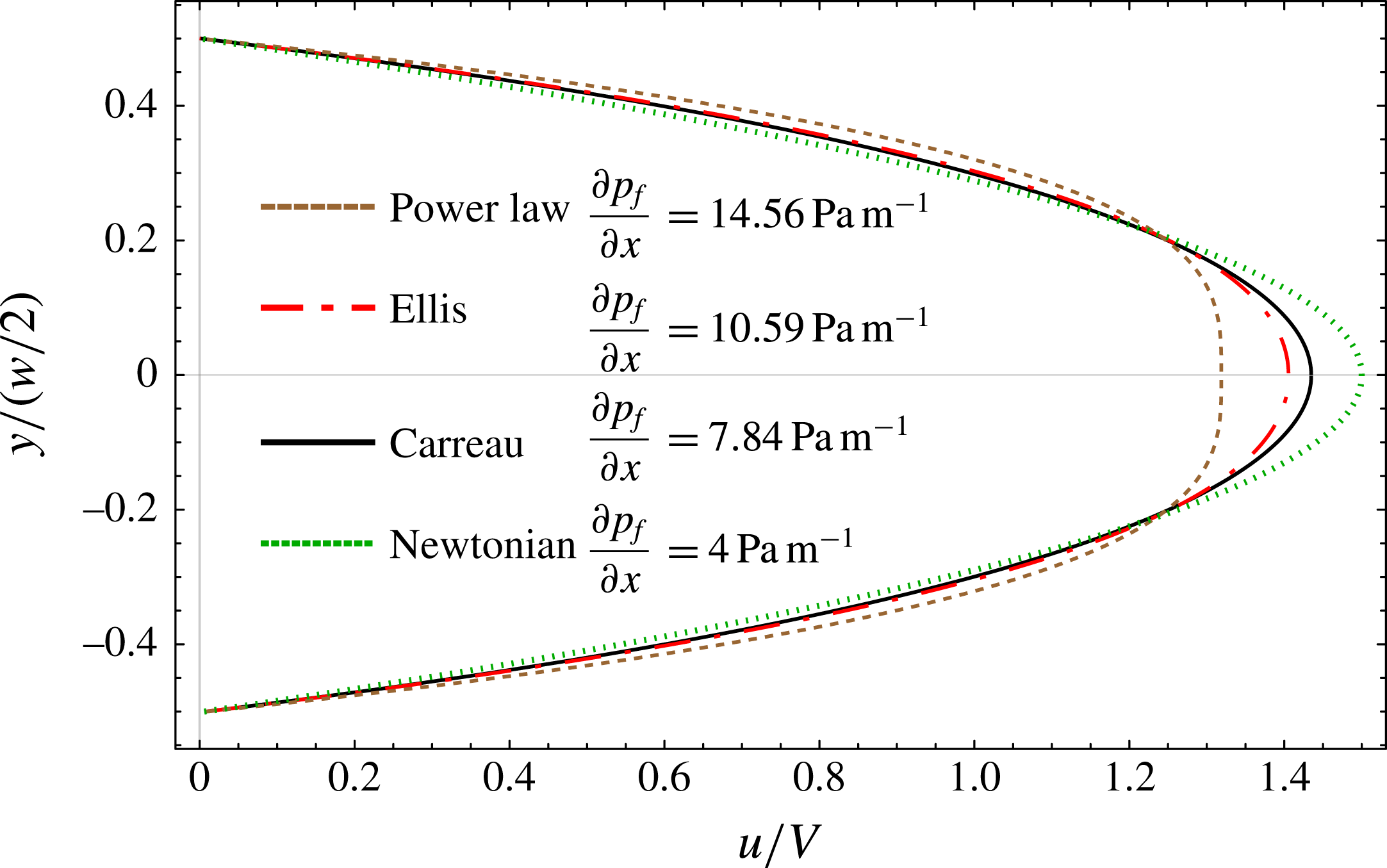
Within a fracture, fluid flow occurs under lubrication condition between parallel plates. For the same average velocity (and the rheological parameters of the HPG fluid listed in table 1), the different rheologies exhibit a different velocity profile across the cross-section of the fracture and the corresponding pressure gradient differs significantly between models as can be seen in figure 2. For that particular example, the power-law fluid has a profile close to a plug flow around the centreline and yield the largest pressure gradient. The Carreau and Ellis models exhibit similar velocity profiles except close to the centreline (but with different pressure gradients). We shall see in the following that these differences between models will impact the solution of the hydraulic fracturing problem.
In order to study the impact of the fluid shear-thinning behaviour on hydraulic fracturing, we focus our analysis on the case of a semi-infinite hydraulic fracture propagating at a constant velocity in a linear elastic and impermeable material. Such a configuration corresponds to a zoom into the tip region of a finite hydraulic fracture (Garagash Reference Garagash2009; Detournay Reference Detournay2016) where a state of plane-strain locally prevails. Such a semi-infinite fracture problem has been extensively studied for the case of a Newtonian fluid (Spence & Sharp Reference Spence and Sharp1985; Desroches et al. Reference Desroches, Detournay, Lenoach, Papanastasiou, Pearson, Thiercelin and Cheng1994; Garagash & Detournay Reference Garagash and Detournay2000; Garagash, Detournay & Adachi Reference Garagash, Detournay and Adachi2011). It has notably enabled to properly quantify the competition between the dissipative processes associated with fracture surface creation and viscous flow. Such a competition is intrinsically linked to the transition between the classical linear elastic fracture mechanics asymptotic region near the fracture tip to a viscosity dominated asymptotic region far from the tip. The extent of the transition being governed by a combination of the fluid viscosity, material fracture toughness, elasticity and fracture velocity.
Our goal is to perform a similar analysis for a shear-thinning fluid. We will use the Carreau rheology to model the complete shear-thinning behaviour of the fluid. We also allow for the possible presence of a fluid-less cavity of a priori unknown length at the fracture tip. Using scaling analysis and a numerical solution of the problem, we aim at understanding the structure of the solution and in particular the extent of the different asymptotic regions (associated with different dissipative mechanisms) as function of the different problem parameters. We will also investigate how an approximation of the shear-thinning behaviour by either the power-law or the Ellis rheological model compares with the more precise Carreau rheology. In other words, how precise one needs to be on the fluid rheology in hydraulic fracturing modelling.
Fluid velocity profiles for a lubrication flow between parallel plates (as it occurs within a fracture) at a given mean velocity
 $\langle u\rangle =V=1~\text{m}~\text{s}^{-1}$
for Carreau, power-law, Ellis and Newtonian fluids. The corresponding fluid pressure gradient is also displayed for each model. The rheological parameters correspond to an HPG fluid (see table 1 for the different models, figure 1 for the rheogram). For the Newtonian velocity profile (dotted green line), the low shear rate viscosity of the HPG is used. Note that the solution for a Carreau fluid is semi-analytical while the solution for the other models can be obtained analytically (see appendices A, B and C for details).

2 Problem formulation
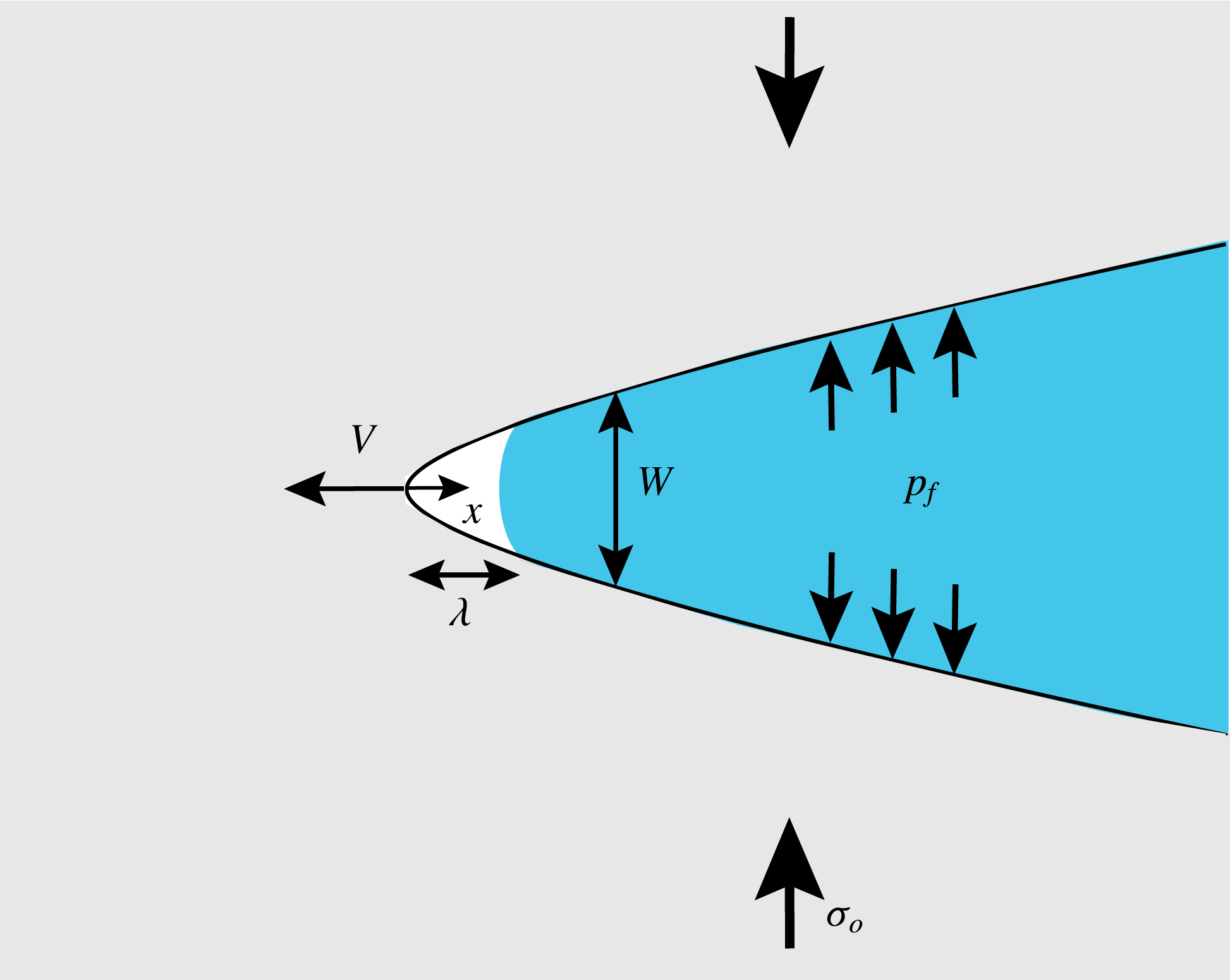
Sketch of a semi-infinite hydraulic fracture propagating at a constant velocity
 $V$
in an impermeable elastic material under a pre-existing normal compressive stress
 $\unicode[STIX]{x1D70E}_{o}$
. A fluid lag zone of a priori unknown length
 $\unicode[STIX]{x1D706}$
adjacent to the fracture tip may be present.

We consider a semi-infinite fluid-driven fracture under plane-strain condition propagating at a constant velocity
 $V$
in an impermeable linear elastic medium (see figure 3). The fracture is propagating normal to the minimum in situ compressive stress
 $\unicode[STIX]{x1D70E}_{o}$
and is internally loaded by the spatially non-uniform fluid pressure
 $p_{f}$
. We also allow for the presence of zone of a priori unknown size
 $\unicode[STIX]{x1D706}$
without fluid at the fracture tip (fluid lag). The fracture is assumed to propagate at a constant velocity
 $V$
in quasi-static equilibrium under a pure opening mode loading. The fracture propagation condition is written as the equality of the mode I stress intensity factor
 $K_{I}$
to the material fracture toughness
 $K_{Ic}$
(Rice Reference Rice1968):
 $$\begin{eqnarray}K_{I}=K_{Ic}.\end{eqnarray}$$
The linear elastic fracture near-tip asymptote for the fracture opening
 $w$
is related to the mode I stress intensity factor
 $K_{I}$
and can be written in view of the propagation condition (2.1) as (Rice Reference Rice1968):
 $$\begin{eqnarray}w(x)=\sqrt{\frac{32}{\unicode[STIX]{x03C0}}}\frac{K_{Ic}}{E^{\prime }}x^{1/2},\quad x\ll 1.\end{eqnarray}$$
In the plane-strain pure tensile configuration of figure 3, the elastic deformation of the material reduces to the following normal traction boundary integral equation between the net pressure loading
 $p(x)=p_{f}(x)-\unicode[STIX]{x1D70E}_{o}$
and the fracture opening
 $w(x)$
(see e.g. Garagash & Detournay Reference Garagash and Detournay2000):
 $$\begin{eqnarray}p(x)=p_{f}(x)-\unicode[STIX]{x1D70E}_{o}=\frac{E^{\prime }}{4\unicode[STIX]{x03C0}}\int _{0}^{\infty }\frac{\unicode[STIX]{x2202}w(s)}{\unicode[STIX]{x2202}s}\frac{\text{d}s}{x-s},\end{eqnarray}$$
where
 $E^{\prime }=E/(1-\unicode[STIX]{x1D708}^{2})$
is the material plane-strain elastic modulus, related to the Young’s modulus
 $E$
and Poisson’s ratio
 $\unicode[STIX]{x1D708}$
. We account explicitly for the possible presence of a region of length
 $\unicode[STIX]{x1D706}$
without fluid near the tip of the fracture due to the possible occurrence of cavitation. This fluid lag zone is filled with fluid vapour and is under a constant pressure equal to the fluid cavitation pressure. Such a cavitation pressure is typically smaller than the confining stress
 $\unicode[STIX]{x1D70E}_{o}$
such that we write the net loading in this lag zone simply as:
 $$\begin{eqnarray}p(x)=p_{cav}-\unicode[STIX]{x1D70E}_{o}\approx -\unicode[STIX]{x1D70E}_{o},\quad x\in [0,\unicode[STIX]{x1D706}].\end{eqnarray}$$
The semi-infinite hydraulic fracture propagates under a constant velocity
 $V$
, such that for an impermeable medium, in the moving coordinates centred on the fracture tip, the fluid continuity equation reduces to (Desroches et al.
Reference Desroches, Detournay, Lenoach, Papanastasiou, Pearson, Thiercelin and Cheng1994):
 $$\begin{eqnarray}V_{f}=V.\end{eqnarray}$$
The width-averaged fluid velocity
 $V_{f}$
is equal to the fracture velocity
 $V$
at any distance from the tip. Under the lubrication approximation, this width-averaged fluid velocity can be related at any
 $x$
to the fracture opening and pressure gradient via the solution of pressure-driven flow between parallel plates. For a Carreau rheology, no analytical formula exists but the solution can be expressed in a similar form that the well-known Poiseuille solution for a Newtonian fluid:
 $$\begin{eqnarray}V=\frac{1}{12\unicode[STIX]{x1D707}_{o}\unicode[STIX]{x1D6E4}(\unicode[STIX]{x1D70F}_{w},n,\unicode[STIX]{x1D707}_{\infty }/\unicode[STIX]{x1D707}_{o},\dot{\unicode[STIX]{x1D6FE}}_{c})}w^{2}\frac{\unicode[STIX]{x2202}p_{f}}{\unicode[STIX]{x2202}x},\quad x\in ]\unicode[STIX]{x1D706},\infty [,\end{eqnarray}$$
where the dimensionless apparent width-averaged viscosity for parallel plates flow
 $\unicode[STIX]{x1D6E4}(\unicode[STIX]{x1D70F}_{w},n,\unicode[STIX]{x1D707}_{\infty }/\unicode[STIX]{x1D707}_{o},\dot{\unicode[STIX]{x1D6FE}}_{c})$
depends nonlinearly on the shear stress at the fracture wall
 $\unicode[STIX]{x1D70F}_{w}=(w/2)|\unicode[STIX]{x2202}p/\unicode[STIX]{x2202}x|$
as well as the rheological parameters of the Carreau model. This dimensionless apparent viscosity requires the solution of the rheological equation at the fracture wall in order to obtain the wall shear rate
 $\dot{\unicode[STIX]{x1D6FE}}_{w}=\unicode[STIX]{x1D70F}_{w}/\unicode[STIX]{x1D707}(\dot{\unicode[STIX]{x1D6FE}}_{w})$
for a given value of wall shear stress (Sochi Reference Sochi2014, Reference Sochi2015) (see appendix A for details). It is interesting to note that an analytical solution exists for the lubrication of a power-law rheology as well as for the Ellis rheological model (Myers Reference Myers2005).
The aim is to solve for both the fracture opening
 $w(x)$
and net pressure
 $p(x)$
profiles as well as the extent of the lag
 $\unicode[STIX]{x1D706}$
as function of the fracture velocity
 $V$
, solid material properties (elastic modulus
 $E^{\prime }$
, fracture toughness
 $K_{Ic}$
) and fluid rheological properties.
3 Scaling
We follow the scaling first introduced by Garagash & Detournay (Reference Garagash and Detournay2000) for the case of a semi-infinite hydraulic fracture driven by a Newtonian fluid. A characteristic viscous length scale
 $L_{\unicode[STIX]{x1D707}_{o}}$
scales all distances, while the fracture width is scaled by
 $\unicode[STIX]{x1D716}L_{\unicode[STIX]{x1D707}_{o}}$
(with
 $\unicode[STIX]{x1D716}$
a small number) and the characteristic pressure is taken as the in situ compressive stress
 $\unicode[STIX]{x1D70E}_{o}$
. We thus define the normalized moving coordinate
 $\unicode[STIX]{x1D709}=x/L_{\unicode[STIX]{x1D707}_{o}}$
and the normalized fracture opening
 $\unicode[STIX]{x1D6FA}(\unicode[STIX]{x1D709})$
, net pressure
 $\unicode[STIX]{x1D6F1}(\unicode[STIX]{x1D709})$
and fluid lag
 $\unicode[STIX]{x1D6EC}$
size as
 $$\begin{eqnarray}w=\unicode[STIX]{x1D716}L_{\unicode[STIX]{x1D707}_{o}}\unicode[STIX]{x1D6FA}(\unicode[STIX]{x1D709}),\quad p=\unicode[STIX]{x1D70E}_{o}\unicode[STIX]{x1D6F1}(\unicode[STIX]{x1D709}),\quad \unicode[STIX]{x1D706}=L_{\unicode[STIX]{x1D707}_{o}}\unicode[STIX]{x1D6EC}.\end{eqnarray}$$
The scaling parameters (
 $L_{\unicode[STIX]{x1D707}_{o}},\unicode[STIX]{x1D716}$
) can be obtained from the elasticity equation (2.3) and the lubrication relation (2.6):
 $L_{\unicode[STIX]{x1D707}_{o}}$
is a fracture characteristic length scale related to the viscosity propagation regime and its expression depends on the fluid rheological model. The small dimensionless parameter
 $\unicode[STIX]{x1D716}$
is independent of the fluid rheology and is defined as the ratio between confining stress and the solid material plane-strain Young’s modulus. For a Carreau rheology, choosing the low shear rate viscosity
 $\unicode[STIX]{x1D707}_{o}$
as a representative value of viscosity, we write similarly to Garagash & Detournay (Reference Garagash and Detournay2000)
 $$\begin{eqnarray}L_{\unicode[STIX]{x1D707}_{o}}=\frac{12\unicode[STIX]{x1D707}_{o}VE^{\prime 2}}{\unicode[STIX]{x1D70E}_{o}^{3}},\quad \unicode[STIX]{x1D716}=\frac{\unicode[STIX]{x1D70E}_{o}}{E^{\prime }}.\end{eqnarray}$$
These scales for the slightly different cases of a power-law and Ellis rheology are discussed in appendices B and C.
The corresponding dimensionless governing equations in that scaling simplify to the following:
-
(i) Elasticity equation relating net pressure to fracture opening
(3.3) $$\begin{eqnarray}\unicode[STIX]{x1D6F1}(\unicode[STIX]{x1D709})=\frac{1}{4\unicode[STIX]{x03C0}}\int _{0}^{\infty }\frac{\unicode[STIX]{x2202}\unicode[STIX]{x1D6FA}(\unicode[STIX]{x1D709}^{\prime })}{\unicode[STIX]{x2202}\unicode[STIX]{x1D709}^{\prime }}\frac{\text{d}\unicode[STIX]{x1D709}^{\prime }}{\unicode[STIX]{x1D709}-\unicode[STIX]{x1D709}^{\prime }}.\end{eqnarray}$$
-
(ii) The fracture propagation expressed as a near-tip width asymptotic
(3.4)where
$$\begin{eqnarray}\unicode[STIX]{x1D6FA}(\unicode[STIX]{x1D709})=\unicode[STIX]{x1D705}\sqrt{\unicode[STIX]{x1D709}}\quad \text{for }\unicode[STIX]{x1D709}\rightarrow 0,\end{eqnarray}$$
$\unicode[STIX]{x1D705}$
is a dimensionless toughness defined in such a scaling as (3.5)
$$\begin{eqnarray}\unicode[STIX]{x1D705}=\sqrt{\frac{8}{3\unicode[STIX]{x03C0}}}\left(\frac{\unicode[STIX]{x1D70E}_{o}}{V\unicode[STIX]{x1D707}_{o}}\right)^{1/2}\frac{K_{Ic}}{E^{\prime }}.\end{eqnarray}$$
-
(iii) The net pressure in the lag region
(3.6)
$$\begin{eqnarray}\unicode[STIX]{x1D6F1}=-1\quad \text{for }\unicode[STIX]{x1D709}\in \left[0,\unicode[STIX]{x1D6EC}\right].\end{eqnarray}$$
-
(iv) The lubrication flow equation
(3.7)
$$\begin{eqnarray}\frac{1}{\displaystyle \unicode[STIX]{x1D6E4}\left(\frac{\unicode[STIX]{x1D6FA}}{2}\left|\frac{\unicode[STIX]{x2202}\unicode[STIX]{x1D6F1}}{\unicode[STIX]{x2202}\unicode[STIX]{x1D709}}\right|,\unicode[STIX]{x1D6FC},n,\unicode[STIX]{x1D707}_{\infty }/\unicode[STIX]{x1D707}_{o}\right)}\unicode[STIX]{x1D6FA}^{2}\frac{\unicode[STIX]{x2202}\unicode[STIX]{x1D6F1}}{\unicode[STIX]{x2202}\unicode[STIX]{x1D709}}=1\text{ for }\unicode[STIX]{x1D709}\in ]\unicode[STIX]{x1D6EC},\infty [.\end{eqnarray}$$


The dimensionless apparent viscosity
 $\unicode[STIX]{x1D6E4}((1/2)\unicode[STIX]{x1D6FA}|\unicode[STIX]{x2202}\unicode[STIX]{x1D6F1}/\unicode[STIX]{x2202}\unicode[STIX]{x1D709}|,\unicode[STIX]{x1D6FC},n,\unicode[STIX]{x1D707}_{\infty }/\unicode[STIX]{x1D707}_{o})$
can be written as a function of the dimensionless fluid shear stress at the wall
 $(\unicode[STIX]{x1D6FA}/2)|\unicode[STIX]{x2202}\unicode[STIX]{x1D6F1}/\unicode[STIX]{x2202}\unicode[STIX]{x1D709}|$
, the fluid shear-thinning index
 $n$
, the viscosity ratio
 $\unicode[STIX]{x1D707}_{\infty }/\unicode[STIX]{x1D707}_{o}$
and a parameter
 $\unicode[STIX]{x1D6FC}$
which is defined as the ratio between the characteristic shear stress at the wall
 $\unicode[STIX]{x1D716}\hspace{2.22198pt}\unicode[STIX]{x1D70E}_{o}$
and the critical fluid shear stress
 $\unicode[STIX]{x1D70F}^{c}=\unicode[STIX]{x1D707}_{o}\dot{\unicode[STIX]{x1D6FE}}_{c}$
corresponding to the critical shear rate
 $\dot{\unicode[STIX]{x1D6FE}}_{c}$
at which the fluid starts to shear thin (see figure 1):
 $$\begin{eqnarray}\unicode[STIX]{x1D6FC}=\frac{\unicode[STIX]{x1D716}\,\unicode[STIX]{x1D70E}_{o}}{\unicode[STIX]{x1D707}_{o}\dot{\unicode[STIX]{x1D6FE}}_{c}}=\frac{\unicode[STIX]{x1D70E}_{o}^{2}}{\unicode[STIX]{x1D707}_{o}\dot{\unicode[STIX]{x1D6FE}}_{c}E^{\prime }}.\end{eqnarray}$$
For typical order of magnitude of the far-field stress
 $\unicode[STIX]{x1D70E}_{o}$
(MPa) and elastic modulus
 $E^{\prime }$
(GPa), such a dimensionless transition shear stress
 $\unicode[STIX]{x1D6FC}$
ranges from
 $10$
for a fluid with a large low shear rate Newtonian plateau (large value of
 $\dot{\unicode[STIX]{x1D6FE}}_{c}$
) to
 $10^{5}$
for a fluid with a shorter transition to a shear-thinning behaviour (small
 $\dot{\unicode[STIX]{x1D6FE}}_{c}$
). The fluid index
 $n$
varies for most of hydraulic fracturing fluids between
 $0.1$
and
 $0.5$
. For a fluid with large shear-thinning magnitude, the viscosity ratio is about
 $10^{-3}$
versus
 $0.1$
for a fluid with a small shear-thinning magnitude.
The dimensionless solution of the problem thus depends on four dimensionless parameters: the dimensionless toughness
 $\unicode[STIX]{x1D705}$
defined in (3.5), dimensionless transition shear stress
 $\unicode[STIX]{x1D6FC}$
(3.8), fluid index
 $n$
and the overall extent of the shear-thinning behaviour of the fluid captured by the ratio between the large and low shear rate viscosity
 $\unicode[STIX]{x1D707}_{\infty }/\unicode[STIX]{x1D707}_{o}$
.
4 Asymptotes
The knowledge of the solution for the case of a Newtonian fluid (Garagash & Detournay Reference Garagash and Detournay2000) as well as the limiting solution for zero-lag/zero toughness for a power-law rheology (Desroches et al. Reference Desroches, Detournay, Lenoach, Papanastasiou, Pearson, Thiercelin and Cheng1994) will provide some guideline to understand how the solution for a Carreau rheology is structured as one moves away from the fracture tip. The different tip asymptotes can be expressed in terms of the following characteristic length scales:
 $$\begin{eqnarray}\ell _{k}=\frac{32}{\unicode[STIX]{x03C0}}\left(\frac{K_{Ic}}{E^{\prime }}\right)^{2},\quad \ell _{m_{o}}=\frac{12\unicode[STIX]{x1D707}_{o}}{E^{\prime }}V,\quad \ell _{m_{n}}=\left(\frac{M^{\prime }}{E^{\prime }}\right)^{1/n}V,\quad \ell _{m_{\infty }}=\frac{12\unicode[STIX]{x1D707}_{\infty }}{E^{\prime }}V,\end{eqnarray}$$
where
 $M^{\prime }=(2^{n+1}(2n+1)^{n}/n^{n})M$
, and
 $M$
is the power-law consistency which is defined from the Carreau parameters as per equation (1.1).
4.1 Near-field asymptote
The near-tip asymptote of the fracture opening is governed by linear elastic fracture mechanics (LEFM). In this region, the fracture width evolves with the square root of distance to the tip and the toughness characteristic length scale
 $\ell _{k}$
(see (4.1)):
 $$\begin{eqnarray}\unicode[STIX]{x1D705}\text{-asymptote}:w_{k}=\ell _{k}^{1/2}x^{1/2}+O(x^{3/2}),\quad p_{k}=-\unicode[STIX]{x1D70E}_{o},\end{eqnarray}$$
which takes the following form in the scaling previously defined:
 $$\begin{eqnarray}\unicode[STIX]{x1D6FA}_{k}=\unicode[STIX]{x1D705}\unicode[STIX]{x1D709}^{1/2}+O(\unicode[STIX]{x1D709}^{3/2}),\quad \unicode[STIX]{x1D6F1}_{k}=-1.\end{eqnarray}$$
For the strictly zero toughness case (
 $\unicode[STIX]{x1D705}=0$
), the width evolves as
 $\unicode[STIX]{x1D709}^{3/2}$
which corresponds to the higher-order term in the linear elastic fracture mechanics asymptotic development (see e.g. Rice Reference Rice1968; Garagash Reference Garagash2009). In the complete problem, the extent of this LEFM region depends on the viscous length scale
 $L_{\unicode[STIX]{x1D707}_{o}}$
as well as the value of the dimensionless toughness (i.e. the corresponding lag size).
4.2 Far-field asymptotes
In the case where both the fluid lag and toughness are negligible (
 $\unicode[STIX]{x1D705}\ll 1,\unicode[STIX]{x1D6EC}\ll 1$
), the behaviour of the solution is governed by the coupling between lubrication flow and elasticity which yields a different power-law dependence of the opening with distance from the tip. The solution for a power-law rheology (for zero lag and zero toughness) have been obtained in Desroches et al. (Reference Desroches, Detournay, Lenoach, Papanastasiou, Pearson, Thiercelin and Cheng1994). Such a solution corresponds to a far-field asymptote valid at a distance from the tip where the effect of dimensionless toughness and the presence of the lag vanishes (see e.g. Garagash & Detournay (Reference Garagash and Detournay2000), Garagash (Reference Garagash2009), Garagash et al. (Reference Garagash, Detournay and Adachi2011) for discussion). For a Carreau rheology, as the average shear rate
 $V/w$
decreases as one moves away from the fracture tip, we can expect to see two or more viscosity dominated asymptotes. Far away from the fracture tip, i.e. for very low shear rate, one should recover the viscosity asymptote for a Newtonian with the low shear rate viscosity (see figure 1), i.e.
 $$\begin{eqnarray}m_{o}\text{-asymptote}(\unicode[STIX]{x1D705}=\unicode[STIX]{x1D6EC}=0):w_{m_{o}}=\unicode[STIX]{x1D6FD}_{o}\ell _{m_{o}}^{1/3}x^{2/3},\quad p_{m_{o}}=-\frac{\unicode[STIX]{x1D6FD}_{o}}{6\sqrt{3}}E^{\prime }\ell _{m_{o}}^{1/3}x^{-1/3},\end{eqnarray}$$
where
 $$\begin{eqnarray}\unicode[STIX]{x1D6FD}_{o}=2^{1/3}\times 3^{5/6}.\end{eqnarray}$$
This
 $m_{o}$
-asymptote in the scaling previously defined in § 3 has the following form:
 $$\begin{eqnarray}\unicode[STIX]{x1D6FA}_{m_{o}}=\unicode[STIX]{x1D6FD}_{o}\unicode[STIX]{x1D709}^{2/3},\quad \unicode[STIX]{x1D6F1}_{m_{o}}=-\frac{\unicode[STIX]{x1D6FD}_{o}}{6\sqrt{3}}\unicode[STIX]{x1D709}^{-1/3}.\end{eqnarray}$$
As we move closer to the fracture tip, the fluid will exhibit shear thinning. The fracture opening should thus eventually follow the viscosity asymptote for a power-law fluid. We will refer to this power-law asymptote – first derived by Desroches et al. (Reference Desroches, Detournay, Lenoach, Papanastasiou, Pearson, Thiercelin and Cheng1994) – as
 $m_{n}$
:
 $$\begin{eqnarray}\displaystyle & \displaystyle w_{m_{n}}=\unicode[STIX]{x1D6FD}_{n}\ell _{m_{n}}^{n/(2+n)}x^{2/(n+2)}, & \displaystyle\end{eqnarray}$$
 $$\begin{eqnarray}\displaystyle & \displaystyle p_{m_{n}}=-\frac{\unicode[STIX]{x1D6FD}_{n}}{2(n+2)}\cot \left(\frac{-2\unicode[STIX]{x03C0}}{n+2}\right)E^{\prime }\ell _{n}^{n/(2+n)}x^{-n/(n+2)}, & \displaystyle\end{eqnarray}$$
where
 $$\begin{eqnarray}\displaystyle \unicode[STIX]{x1D6FD}_{n}=\left(2\frac{(n+2)^{2}}{n}\tan \left(\frac{-2\unicode[STIX]{x03C0}}{n+2}\right)\right)^{1/(n+2)}. & & \displaystyle\end{eqnarray}$$
We can re-express this asymptote using the expression of the power-law consistency
 $M$
as function of the Carreau rheological parameters (see (1.1)). Moreover, using the low shear rate scaling defined in the § 3, such
 $m_{n}$
asymptote
 $\displaystyle (\unicode[STIX]{x1D705}=\unicode[STIX]{x1D6EC}=0)$
reads:
 $$\begin{eqnarray}\unicode[STIX]{x1D6FA}_{m_{n}}=\unicode[STIX]{x1D6FC}^{(n-1)/(n+2)}\unicode[STIX]{x1D6FD}_{\unicode[STIX]{x1D707}}\unicode[STIX]{x1D6FD}_{n}\unicode[STIX]{x1D709}^{2/(n+2)},\quad \unicode[STIX]{x1D6F1}_{m_{n}}=-\frac{\unicode[STIX]{x1D6FC}^{(n-1)/(n+2)}\unicode[STIX]{x1D6FD}_{\unicode[STIX]{x1D707}}\unicode[STIX]{x1D6FD}_{n}}{2(n+2)}\cot \left(\frac{-2\unicode[STIX]{x03C0}}{n+2}\right)\unicode[STIX]{x1D709}^{-n/(n+2)},\end{eqnarray}$$
where
 $$\begin{eqnarray}\unicode[STIX]{x1D6FD}_{\unicode[STIX]{x1D707}}=\left(\left(\frac{2n+1}{6n}\right)^{n}\frac{1+\unicode[STIX]{x1D707}_{\infty }/\unicode[STIX]{x1D707}_{o}}{\left(\sqrt{2^{-2/(n-1)}-1}\right)^{n-1}}\right)^{1/(n+2)}.\end{eqnarray}$$
Finally, as we move closer to the fracture tip, for larger average shear rate, it may well be that another Newtonian viscous asymptote linked to the Newtonian behaviour at large shear rate
 $\unicode[STIX]{x1D707}_{\infty }$
could be observed (see (4.12)). In the low shear rate scaling, this large shear rate asymptote is given by:
 $$\begin{eqnarray}m_{\infty }\text{-asymptote }(\unicode[STIX]{x1D705}=\unicode[STIX]{x1D6EC}=0):w_{m_{\infty }}=\unicode[STIX]{x1D6FD}_{o}\ell _{m_{\infty }}^{1/3}x^{2/3},\quad p_{m_{\infty }}=-\frac{\unicode[STIX]{x1D6FD}_{o}}{6\sqrt{3}}E^{\prime }\ell _{m_{\infty }}^{1/3}x^{-1/3}\end{eqnarray}$$
or alternatively in dimensionless form in the lag scaling:
 $$\begin{eqnarray}\unicode[STIX]{x1D6FA}_{m_{\infty }}=\unicode[STIX]{x1D6FD}_{o}\left(\unicode[STIX]{x1D707}_{\infty }/\unicode[STIX]{x1D707}_{o}\right)^{1/3}\unicode[STIX]{x1D709}^{2/3},\quad \unicode[STIX]{x1D6F1}_{m_{\infty }}=-\frac{\unicode[STIX]{x1D6FD}_{o}}{6\sqrt{3}}\left(\unicode[STIX]{x1D707}_{\infty }/\unicode[STIX]{x1D707}_{o}\right)^{1/3}\unicode[STIX]{x1D709}^{-1/3}.\end{eqnarray}$$
The evolution of the complete solution between these different asymptotes as well as the extent of the regions where these asymptotes may be valid will depend on the values of the different dimensionless parameters governing the problem, namely
 $\unicode[STIX]{x1D705},\unicode[STIX]{x1D6FC},n$
and
 $\unicode[STIX]{x1D707}_{\infty }/\unicode[STIX]{x1D707}_{o}$
.
5 Numerical scheme
We develop a numerical scheme for the solution of the complete problem for a given set of dimensionless parameters (
 $\unicode[STIX]{x1D705},\unicode[STIX]{x1D6FC},n$
and
 $\unicode[STIX]{x1D707}_{\infty }/\unicode[STIX]{x1D707}_{o}$
). In our simulation, following Garagash & Detournay (Reference Garagash and Detournay2000), we actually prescribe the dimensionless lag size
 $\unicode[STIX]{x1D6EC}$
such that the domain where the lubrication equation is enforced is known a priori. We thus solve for the corresponding value of dimensionless toughness
 $\unicode[STIX]{x1D705}$
, as well as dimensionless pressure and opening.
We use a Gauss–Chebyshev quadrature for the discretization of the elasticity equation. We embed the linear fracture mechanics asymptote directly in the discretization of the dislocation density:
 $$\begin{eqnarray}\frac{\text{d}\unicode[STIX]{x1D6FA}}{\text{d}\unicode[STIX]{x1D709}}=\frac{\unicode[STIX]{x1D705}}{\sqrt{\unicode[STIX]{x1D709}}}+\sqrt{\unicode[STIX]{x1D709}}\unicode[STIX]{x1D719}(\unicode[STIX]{x1D709}).\end{eqnarray}$$
We also perform the following changes of coordinates to map the semi-infinite interval
 $\unicode[STIX]{x1D709}\in [0,\infty [$
to
 $v\in [-1,1]$
so that the Gauss–Chebyshev quadrature becomes applicable to the numerical solution (Ioakimidis & Theocaris Reference Ioakimidis and Theocaris1980; Viesca & Garagash Reference Viesca and Garagash2015)
 $$\begin{eqnarray}\unicode[STIX]{x1D709}=\frac{1+v}{1-v}\end{eqnarray}$$
in order to discretize the elasticity equation using a Gauss–Chebyshev quadrature of the third kind at
 $N$
collocation points:
 $$\begin{eqnarray}\frac{\unicode[STIX]{x1D6F1}[\unicode[STIX]{x1D709}(v_{j})]}{1-v_{j}}=\frac{1}{4\unicode[STIX]{x03C0}}\mathop{\sum }_{i=1}^{N}\frac{A_{i}}{1-u_{i}}\frac{\unicode[STIX]{x1D719}[s(u_{i})]}{v_{j}-u_{i}},\end{eqnarray}$$
where
 $u_{i}=\cos (\unicode[STIX]{x03C0}(i-0.5)/N)$
and
 $A_{i}=(\unicode[STIX]{x03C0}/N)(1+u_{i})$
. The net pressure is evaluated at points
 $v_{j}=\cos (\unicode[STIX]{x03C0}j/N)$
for
 $j=1,2,\ldots ,N$
, whereas the dislocation density
 $\unicode[STIX]{x1D719}[s(u_{i})]$
is evaluated at points
 $u_{i}$
for
 $i=1,2,\ldots ,N$
.
The lubrication equation is discretized at the mid distance
 $\unicode[STIX]{x1D709}_{i+1/2}$
between net pressure collocation points, and the pressure gradient is approximated by centred finite difference. The discretization of (3.7) is thus:
 $$\begin{eqnarray}\unicode[STIX]{x1D6FA}^{2}(\unicode[STIX]{x1D709}_{i+1/2})\frac{\unicode[STIX]{x1D6F1}(\unicode[STIX]{x1D709}_{i+1})-\unicode[STIX]{x1D6F1}(\unicode[STIX]{x1D709}_{i})}{\unicode[STIX]{x1D709}_{i+1}-\unicode[STIX]{x1D709}_{i}}=\unicode[STIX]{x1D6E4}\left(\frac{\unicode[STIX]{x1D6FA}(\unicode[STIX]{x1D709}_{i+1/2})}{2}\frac{\unicode[STIX]{x1D6F1}(\unicode[STIX]{x1D709}_{i+1})-\unicode[STIX]{x1D6F1}(\unicode[STIX]{x1D709}_{i})}{\unicode[STIX]{x1D709}_{i+1}-\unicode[STIX]{x1D709}_{i}},\unicode[STIX]{x1D6FC},n,\unicode[STIX]{x1D707}_{\infty }/\unicode[STIX]{x1D707}_{o}\right).\end{eqnarray}$$
The opening
 $\unicode[STIX]{x1D6FA}(\unicode[STIX]{x1D709}_{i+1/2})$
at
 $\unicode[STIX]{x1D709}_{i+1/2}$
is evaluated from a linear interpolation of the opening evaluated at
 $\unicode[STIX]{x1D709}_{i}$
and
 $\unicode[STIX]{x1D709}_{i+1}$
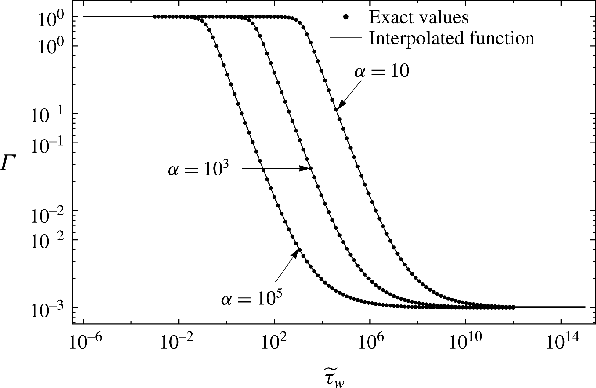
. The nonlinear tangent viscosity
 $\unicode[STIX]{x1D6E4}$
function of the wall shear stress is estimated from the interpolated function built for the given values of
 $\unicode[STIX]{x1D6FC},n$
and
 $\unicode[STIX]{x1D707}_{\infty }/\unicode[STIX]{x1D707}_{o}$
over the whole range of dimensionless wall shear stress (see appendix A). The net pressure
 $\unicode[STIX]{x1D6F1}$
is directly set in the lag zone for the collocation points
 $i\in [1,N_{\unicode[STIX]{x1D6EC}}]$
where
 $N_{\unicode[STIX]{x1D6EC}}$
is the number of points in the lag region:
 $$\begin{eqnarray}\unicode[STIX]{x1D6F1}(\unicode[STIX]{x1D709}_{i})=-1,\end{eqnarray}$$
while at infinity the net pressure is set to zero, i.e. we set the following constraint at the last collocation point
 $$\begin{eqnarray}\unicode[STIX]{x1D6F1}(\unicode[STIX]{x1D709}_{N})=0.\end{eqnarray}$$
It follows that the solution for the fracture opening
 $\unicode[STIX]{x1D6FA}$
is positive while the net pressure
 $\unicode[STIX]{x1D6F1}$
is everywhere negative. This is a direct consequence of the semi-infinite nature of this problem where pressure is determined up to a constant (see e.g. Garagash & Detournay (Reference Garagash and Detournay2000) for discussion).
The resulting nonlinear system of equations is solved via a quasi-Newton root-finding scheme using the dimensionless net pressure at the collocation points and
 $\unicode[STIX]{x1D705}$
as the primary unknown variables. The algorithm has been implemented in Mathematica with computational accuracy in mind (but not efficiency). The numerical results reported in the remaining of this paper have been obtained with a total number of collocation points between 1600 and 3000. Convergence of the lubrication equation (5.4) has been obtained with an accuracy of
 $10^{-8}$
on the norm of the residuals. A simulation typically takes from few minutes up to three hours on a modern personal computer (Macbook Pro, Early 2015, 2.9 GHz Intel core i5) depending on the prescribed size of the lag, the amplitude of shear thinning and the number of collocation points.
6 Results for a finite fluid lag
6.1 Effect of dimensionless toughness
$\unicode[STIX]{x1D705}$

We first investigate the effect of dimensionless toughness
 $\unicode[STIX]{x1D705}$
for a given set of rheological dimensionless parameters representative of a Carreau fluid:
 $\unicode[STIX]{x1D707}_{\infty }/\unicode[STIX]{x1D707}_{o}=10^{-3},n=0.5,$
and
 $\unicode[STIX]{x1D6FC}=10^{2}$
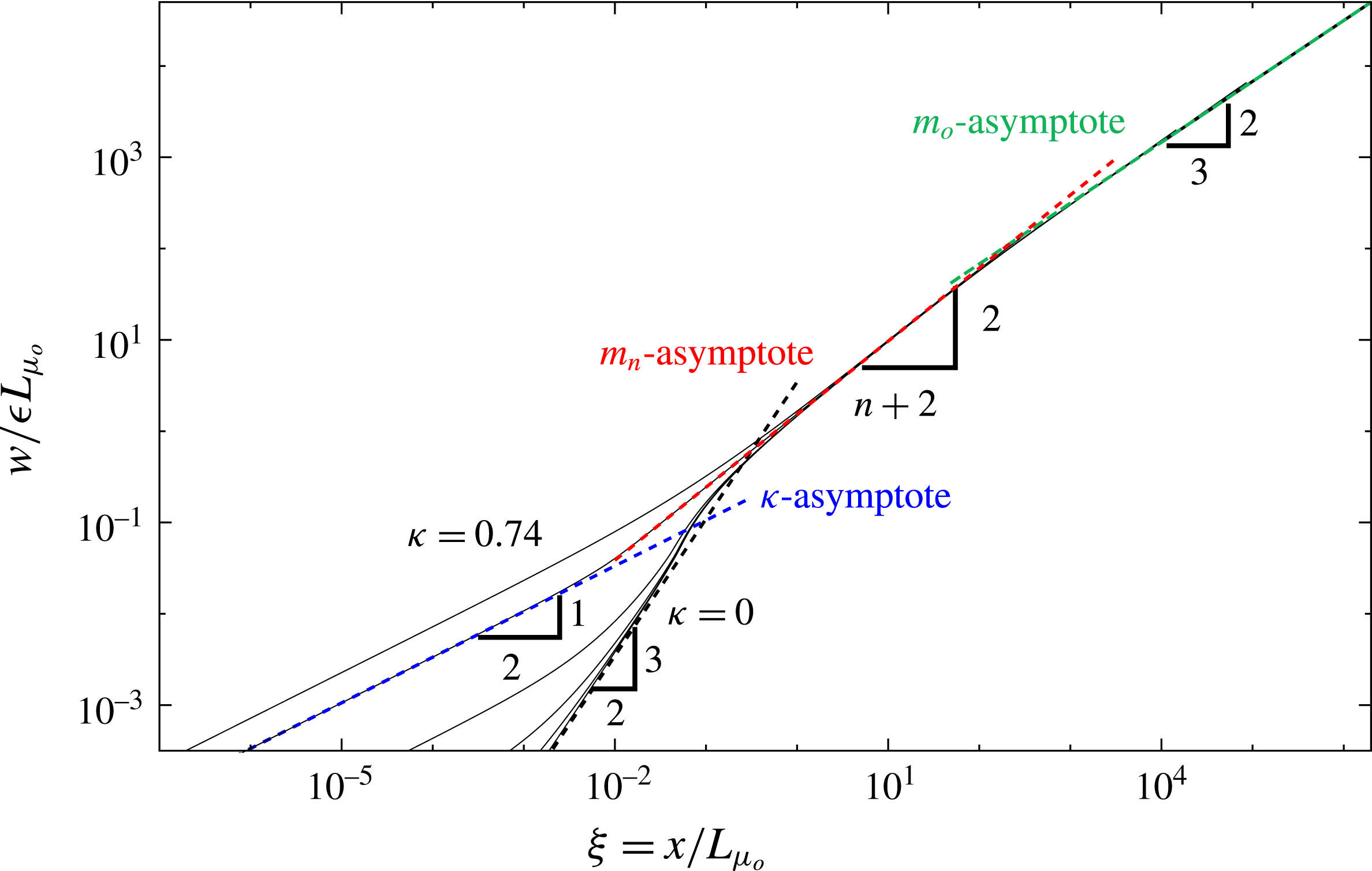
. The profile of dimensionless fracture opening with distance from the tip for different values of dimensionless lag size/ dimensionless toughness is displayed in figure 4, while the corresponding dimensionless net pressure profiles (in semi-log) and the apparent viscosity
 $\unicode[STIX]{x1D6E4}$
are displayed in figures 5 and 6. We can directly observe the extent of the lag on the net pressure profiles which depart from the value
 $\unicode[STIX]{x1D6F1}=-1$
at the fluid front
 $\unicode[STIX]{x1D709}=\unicode[STIX]{x1D6EC}$
. The relation between the dimensionless toughness and the dimensionless lag size for these simulations are better grasped in figure 7. The dimensionless lag size
 $\unicode[STIX]{x1D6EC}$
is decreasing function of dimensionless toughness
 $\unicode[STIX]{x1D705}$
. This is similar to the Newtonian case (see Garagash & Detournay Reference Garagash and Detournay2000) with the difference that for a given value of dimensionless toughness, due to shear thinning, the dimensionless lag is always smaller compared to the Newtonian case (see figure 10 for more simulations with different shear-thinning index
 $n$
, and figure 8 for different transition shear-stress
 $\unicode[STIX]{x1D6FC}$
).
Dimensionless fracture opening
 $w/\unicode[STIX]{x1D716}L_{\unicode[STIX]{x1D707}_{o}}$
along the fracture for
 $\unicode[STIX]{x1D705}=0,0.002,0.008,0.043,0.33,0.74$
(with corresponding lag size
 $\unicode[STIX]{x1D6EC}=0.049,0.048,0.047,0.041,0.008,8.3\times 10^{-8}$
) in log–log scale for
 $\unicode[STIX]{x1D6FC}=10^{2}$
,
 $\unicode[STIX]{x1D707}_{\infty }/\unicode[STIX]{x1D707}_{o}=10^{-3}$
, and
 $n=0.5$
. The dashed lines correspond to the asymptotic solution in the toughness dominated regime (
 $\unicode[STIX]{x1D705}$
-asymptote), power-law viscosity regime (
 $m_{n}$
-asymptote) and low shear rate Newtonian viscosity regime (
 $m_{o}$
-asymptote).

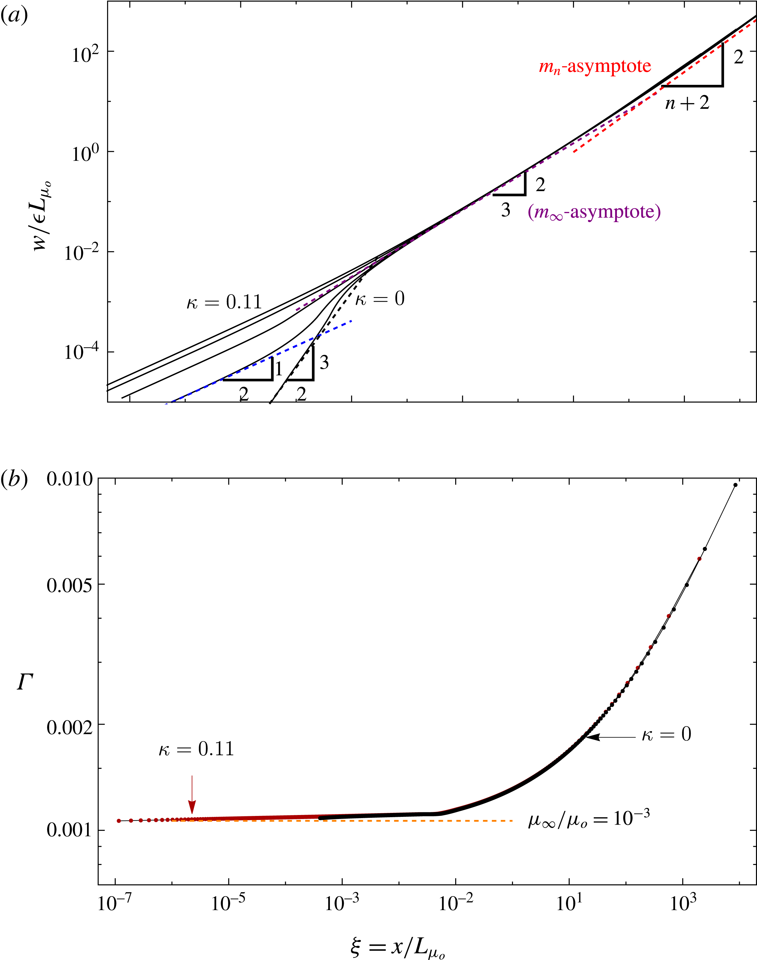
The dimensionless opening profiles (figure 4) also evolve in a similar way to that in the Newtonian case with a region dominated by the LEFM toughness
 $\unicode[STIX]{x1D705}$
-asymptote (4.3) near the fracture tip (for
 $x\ll L_{\unicode[STIX]{x1D707}_{o}}$
) and a region in the far field (for
 $x\gg L_{\unicode[STIX]{x1D707}_{o}}$
) dominated by the low shear rate viscosity asymptote
 $m_{o}$
(4.6). However, here due to the shear-thinning nature of the Carreau rheology, an intermediate region following the power-law dominated asymptote
 $m_{n}$
can be observed for intermediate distances between the LEFM near-tip region and the far-field low shear rate viscosity region. It is worth noting the particularity of the zero toughness case (
 $\unicode[STIX]{x1D705}=0$
) for which the dimensionless lag is maximum and the opening in the near-tip LEFM region evolves as
 $\unicode[STIX]{x1D709}^{3/2}$
(see figure 4).
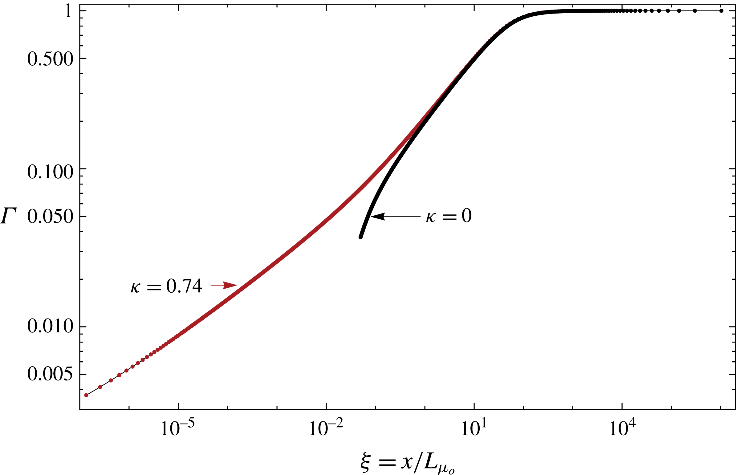
Dimensionless apparent viscosity
 $\unicode[STIX]{x1D6E4}$
along the fracture starting from the fluid front
 $\unicode[STIX]{x1D709}=\unicode[STIX]{x1D6EC}$
for
 $\unicode[STIX]{x1D705}=0$
(
 $\unicode[STIX]{x1D6EC}=0.049$
) and
 $\unicode[STIX]{x1D705}=0.74$
(
 $\unicode[STIX]{x1D6EC}=8.3\times 10^{-8}$
) in log–log scale for
 $\unicode[STIX]{x1D6FC}=10^{2}$
,
 $\unicode[STIX]{x1D707}_{\infty }/\unicode[STIX]{x1D707}_{o}=10^{-3}$
, and
 $n=0.5$
.

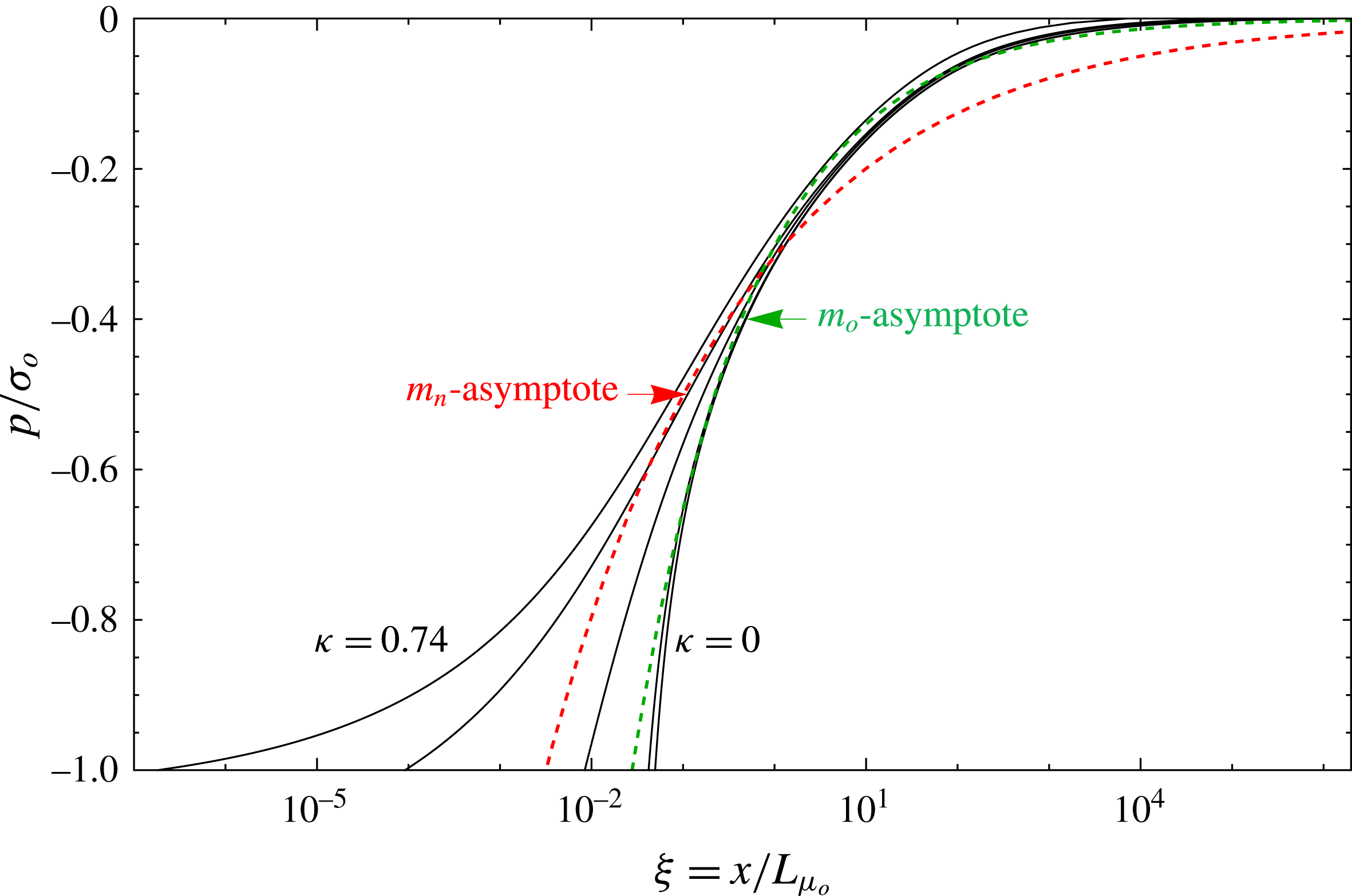
Dimensionless fluid pressure
 $p/\unicode[STIX]{x1D70E}_{o}$
along the fracture for
 $\unicode[STIX]{x1D705}=0,0.002,0.008,0.043,0.33,0.74$
in semi-log scale for
 $\unicode[STIX]{x1D6FC}=10^{2}$
,
 $\unicode[STIX]{x1D707}_{\infty }/\unicode[STIX]{x1D707}_{o}=10^{-3}$
, and
 $n=0.5$
. The dashed lines correspond to the asymptotic solution of pressure in the power-law viscosity regime (
 $m_{n}$
-asymptote) and in the Newtonian viscosity regime (
 $m_{o}$
-asymptote).

The same evolution can be seen in the net pressure profiles (figure 6). The different viscosity regimes as function of distance from the tip are also visible in figure 5 where the dimensionless apparent viscosity
 $\unicode[STIX]{x1D6E4}$
is plotted along the fracture for the two cases
 $\unicode[STIX]{x1D705}=0$
(
 $\unicode[STIX]{x1D6EC}=0.049$
) and
 $\unicode[STIX]{x1D705}=0.74$
(
 $\unicode[STIX]{x1D6EC}=8.3\times 10^{-8}$
). The largest shear rate and therefore the lowest tangent apparent viscosity is always located at the fluid front. For the largest lag case, a smaller shear-thinning region can be observed (see figure 5). On the other hand, for a very small lag (
 $\unicode[STIX]{x1D705}=0.74$
), the fluid strongly shear thin, although the value of the tangent viscosity at the fluid front (
 $\unicode[STIX]{x1D709}=\unicode[STIX]{x1D6EC}$
) remains larger than the large shear rate value
 $\unicode[STIX]{x1D707}_{\infty }/\unicode[STIX]{x1D707}_{o}$
. It is important to note that the large shear rate asymptote is absent for all the simulations performed with this given set of rheological parameters (
 $n=0.5$
,
 $\unicode[STIX]{x1D6FC}=10^{2}$
, and
 $\unicode[STIX]{x1D707}_{\infty }/\unicode[STIX]{x1D707}_{o}=10^{-3}$
).
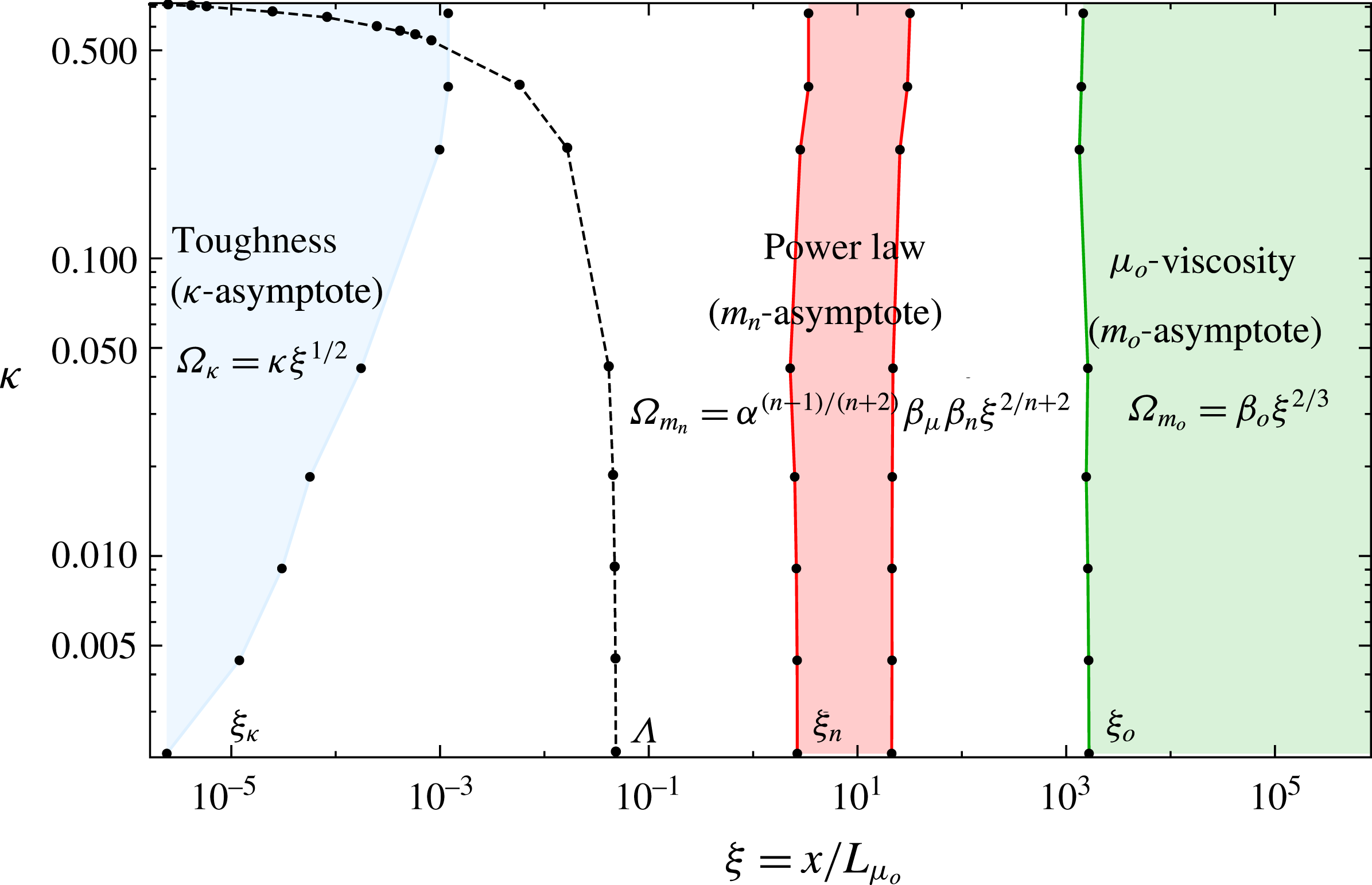
Extent of the regions where the numerical solution can be approximated by the different asymptotes (
 $\unicode[STIX]{x1D705}$
-asymptote,
 $m_{n}$
-asymptote and
 $m_{o}$
-asymptote) with accuracy of
 $10^{-2}$
as function of dimensionless toughness with
 $\unicode[STIX]{x1D6FC}=10^{2},\unicode[STIX]{x1D707}_{\infty }/\unicode[STIX]{x1D707}_{o}=10^{-3},n=0.5$
. The position of the fluid lag is also displayed for comparisons.

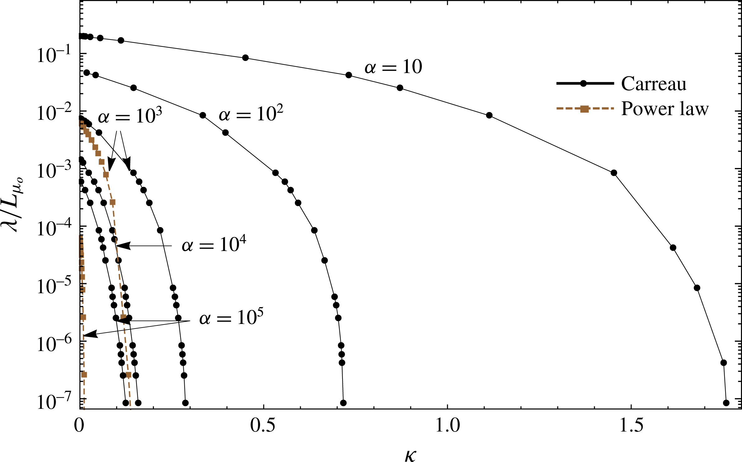
Dimensionless lag length
 $\unicode[STIX]{x1D706}/L_{\unicode[STIX]{x1D707}_{o}}$
versus the dimensionless toughness
 $\unicode[STIX]{x1D705}$
for a Carreau rheology for different values of
 $\unicode[STIX]{x1D6FC}$
(
 $\unicode[STIX]{x1D707}_{\infty }/\unicode[STIX]{x1D707}_{o}=10^{-3},n=0.5$
). The corresponding results for a power-law rheology are also displayed for
 $\unicode[STIX]{x1D6FC}=10^{5}$
and
 $\unicode[STIX]{x1D6FC}=10^{3}$
for comparison.

The relative extent of these different asymptotic regions depends on the values of the dimensionless problem parameters. In order to picture the variation of the size of these asymptotic regions as function of dimensionless toughness
 $\unicode[STIX]{x1D705}$
, we determine from our numerical results the spatial locations (
 $\unicode[STIX]{x1D709}_{\unicode[STIX]{x1D705}}$
,
 $\unicode[STIX]{x1D709}_{n}$
and
 $\unicode[STIX]{x1D709}_{o}$
) where our numerical results for the fracture opening are within 1 % of these different asymptotes. The results are displayed in figure 7 for that same set of parameters (
 $\unicode[STIX]{x1D6FC}=10^{2}$
,
 $\unicode[STIX]{x1D707}_{\infty }/\unicode[STIX]{x1D707}_{o}=10^{-3}$
, and
 $n=0.5$
) where we see that the extent of the power-law and low shear rate viscosity regions do not significantly change with dimensionless toughness while the LEFM near-tip region shrinks when the dimensionless toughness decreases (and the lag size increases) as expected. We also see that the fluid lag region is always localized in the toughness asymptotic region (for large
 $\unicode[STIX]{x1D705}$
) – or in the transition between the toughness and power-law region (small
 $\unicode[STIX]{x1D705}$
).
6.2 Effect of the dimensionless transition shear stress
$\unicode[STIX]{x1D6FC}$

The value of the dimensionless transition shear stress ratio
 $\unicode[STIX]{x1D6FC}$
reflects the extent of the low shear rate plateau:
 $\unicode[STIX]{x1D6FC}$
is inversely proportional to the critical shear rate
 $\dot{\unicode[STIX]{x1D6FE}}_{c}$
(see (3.8)). For large
 $\unicode[STIX]{x1D6FC}$
, the fluid shear thins faster and as a result the dimensionless lag is getting smaller for a similar value of dimensionless toughness. This can be clearly seen in figure 8 where the
 $\unicode[STIX]{x1D6EC}-\unicode[STIX]{x1D705}$
evolution is plotted for different values of
 $\unicode[STIX]{x1D6FC}$
for
 $n=0.5$
and
 $\unicode[STIX]{x1D707}_{\infty }/\unicode[STIX]{x1D707}_{o}=10^{-3}$
.
More interestingly, the structure of the solution also changes for larger value of
 $\unicode[STIX]{x1D6FC}$
. We present in figure 9 the evolution of the dimensionless fracture opening and apparent viscosity for a large dimensionless transition shear stress ratio
 $\unicode[STIX]{x1D6FC}=10^{7}$
while the shear-thinning index
 $n$
and extent
 $\unicode[STIX]{x1D707}_{\infty }/\unicode[STIX]{x1D707}_{o}$
are kept the same as in the previous section:
 $n=0.5$
and
 $\unicode[STIX]{x1D707}_{\infty }/\unicode[STIX]{x1D707}_{o}=10^{-3}$
. For this case, the dimensionless opening profiles (for different
 $\unicode[STIX]{x1D705}$
) involve an additional viscosity asymptote corresponding to the large shear rate
 $m_{\infty }$
viscosity asymptote located in between the toughness and shear-thinning asymptotic regions. Even though the toughness region increases with
 $\unicode[STIX]{x1D705}$
, the validity of the
 $m_{\infty }$
asymptote roughly starts at the same distance from the fracture tip
 $\unicode[STIX]{x1D709}\simeq 0.01$
for all values of
 $\unicode[STIX]{x1D705}$
. This can also be clearly seen in the apparent viscosity profiles depicted on figure 9(b): the apparent viscosity close to the fluid front reaches the large shear rate value at about
 $\unicode[STIX]{x1D709}\approx 0.1$
.
The opening in the shear-thinning region actually does not coincide exactly with the
 $m_{n}$
power-law asymptote (red dashed line in figure 9
a). This is the case for all dimensionless toughness values. This difference is rooted in the behaviour of the Carreau viscosity at large shear rate. If we zoom in the region of large
 $\dot{\unicode[STIX]{x1D6FE}}>1000$
in figure 1, one can observe that the transition from the power-law behaviour to the Newtonian high shear rate behaviour occurs over a large range of shear rate for a Carreau rheology. This large transition region can be clearly seen in the apparent viscosity profiles (figure 9
b), where it departs from the large shear rate value at
 $\unicode[STIX]{x1D709}\approx 0.1$
and reaches the power-law branch at approximately
 $\unicode[STIX]{x1D709}\approx 100$
(or more). As a result the opening profile beyond the large shear rate viscosity asymptotic region are shifted from the
 $m_{n}$
power-law asymptote although they exhibit a similar power exponent. This difference is negligible for sufficiently small dimensionless shear stress
 $\unicode[STIX]{x1D6FC}$
as observed in the previous section (see e.g. figure 4), where the large shear rate viscosity asymptote was not visible. The difference between the Carreau opening profile and the power-law asymptote in the shear-thinning region becomes more significant for large
 $\unicode[STIX]{x1D6FC}$
. It is also worthwhile to point out that for the simulations for
 $\unicode[STIX]{x1D6FC}=10^{7}$
reported in figure 9(a), the extent of our computational domain (
 $\unicode[STIX]{x1D709}_{max}=10^{4}$
) was not sufficient to observe the low shear rate asymptotic region.
It is also worth noting that the value of dimensionless toughness (and thus the extent of the lag region) has an effect limited to the near-tip region, such that the transition between the different far-field viscosity asymptotes are not influenced by
 $\unicode[STIX]{x1D705}$
.
(a) Dimensionless fracture opening
 $w/\unicode[STIX]{x1D716}L_{\unicode[STIX]{x1D707}_{o}}$
along the fracture for
 $\unicode[STIX]{x1D705}=0,0.013,0.045,0.085,0.11$
(with corresponding lag size
 $\unicode[STIX]{x1D6EC}=0.0004,0.00025,5.8\times 10^{-5},2.5\times 10^{-6},8.3\times 10^{-8}$
) in log–log scale for
 $\unicode[STIX]{x1D6FC}=10^{7}$
,
 $\unicode[STIX]{x1D707}_{\infty }/\unicode[STIX]{x1D707}_{o}=10^{-3}$
and
 $n=0.5$
(the dashed lines correspond to the asymptotic solution of opening in the toughness dominated regime (
 $\unicode[STIX]{x1D705}$
-asymptote), high shear rate Newtonian viscosity regime (
 $m_{\infty }$
-asymptote) and the power-law viscosity regime (
 $m_{n}$
-asymptote)). (b) Corresponding dimensionless apparent viscosity
 $\unicode[STIX]{x1D6E4}$
starting from the fluid front
 $\unicode[STIX]{x1D709}=\unicode[STIX]{x1D6EC}$
for
 $\unicode[STIX]{x1D705}=0,0.11$
.

6.3 Effect of the fluid shear-thinning index
$n$

The shear-thinning index
 $n$
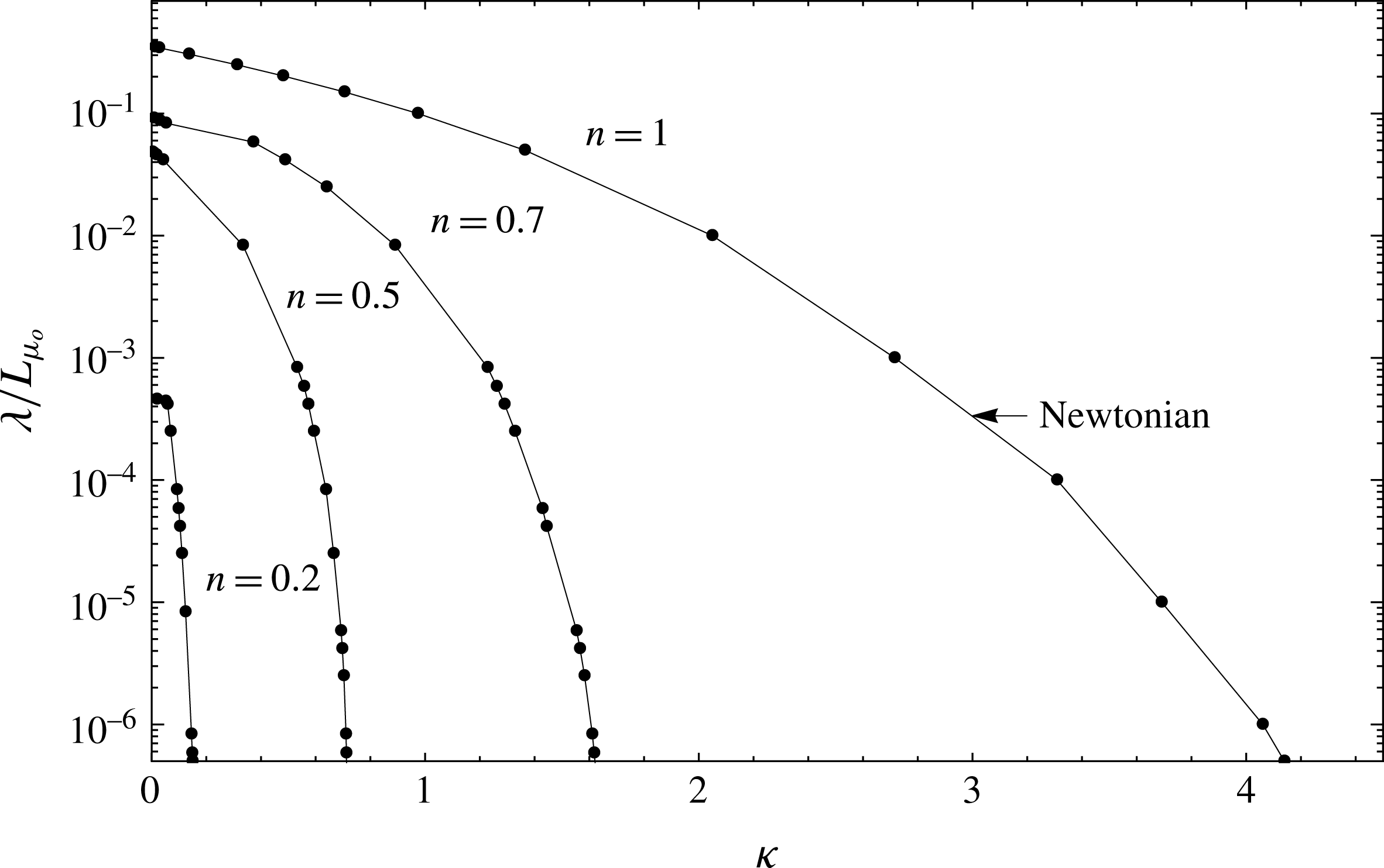
dictates how fast the Carreau fluid transition from the low to high shear rate viscosity. For the same value of dimensionless toughness
 $\unicode[STIX]{x1D705}$
, same shear-thinning extent
 $\unicode[STIX]{x1D707}_{\infty }/\unicode[STIX]{x1D707}_{o}$
and transition shear stress
 $\unicode[STIX]{x1D6FC}$
, a smaller shear-thinning index results in a significantly smaller dimensionless fluid lag as can be seen in figure 10. This result is expected as the extent of the fluid lag is governed mostly by the value of the apparent viscosity near the fluid front. The apparent viscosity actually gets toward the large shear rate limit
 $\unicode[STIX]{x1D707}_{\infty }/\unicode[STIX]{x1D707}_{o}$
near the fluid front for small
 $n$
(steeper shear-thinning branch).
Dimensionless lag length
 $\unicode[STIX]{x1D706}/L_{\unicode[STIX]{x1D707}_{o}}$
versus the dimensionless toughness
 $\unicode[STIX]{x1D705}$
for different values of
 $n$
, (
 $\unicode[STIX]{x1D707}_{\infty }/\unicode[STIX]{x1D707}_{o}=10^{-3},\unicode[STIX]{x1D6FC}=10^{2}$
).

6.4 Effect of the viscosity ratio
$\unicode[STIX]{x1D707}_{\infty }/\unicode[STIX]{x1D707}_{o}$

The overall magnitude of the shear-thinning behaviour (between low and high shear rate) is governed by the ratio
 $\unicode[STIX]{x1D707}_{\infty }/\unicode[STIX]{x1D707}_{o}$
. We have so far set this ratio to
 $10^{-3}$
, a value corresponding to a relatively large shear-thinning magnitude. We now vary this ratio as well as the dimensionless toughness while keeping
 $\unicode[STIX]{x1D6FC}=10^{3}$
and
 $n=0.5$
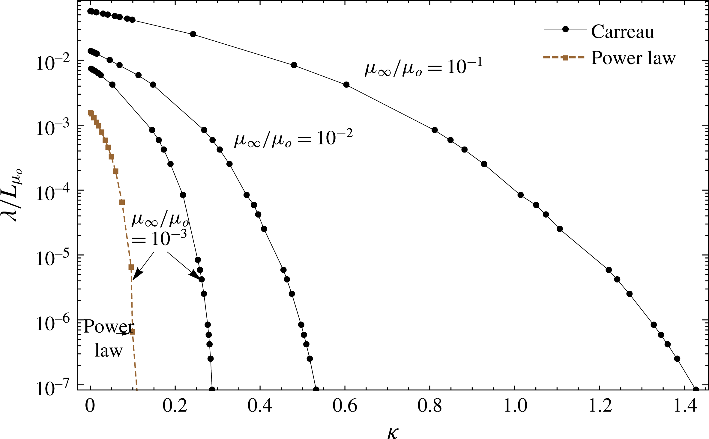
. The lag size–dimensionless toughness relation for different values of
 $\unicode[STIX]{x1D707}_{\infty }/\unicode[STIX]{x1D707}_{o}$
can be seen in figure 11. As expected, the fluid lag is smaller for smaller
 $\unicode[STIX]{x1D707}_{\infty }/\unicode[STIX]{x1D707}_{o}$
(larger shear-thinning magnitude). For
 $\unicode[STIX]{x1D707}_{\infty }/\unicode[STIX]{x1D707}_{o}=1$
, we obviously recover the Newtonian case.
Dimensionless lag length
 $\unicode[STIX]{x1D706}/L_{\unicode[STIX]{x1D707}_{o}}$
versus the dimensionless toughness
 $\unicode[STIX]{x1D705}$
for a Carreau rheology with respect to
 $\unicode[STIX]{x1D707}_{\infty }/\unicode[STIX]{x1D707}_{o}$
(
 $\unicode[STIX]{x1D6FC}=10^{3},n=0.5$
). The results for a power-law rheology are also displayed for
 $\unicode[STIX]{x1D707}_{\infty }/\unicode[STIX]{x1D707}_{o}=10^{-3}$
.

6.5 Comparison between the Carreau, power-law and Ellis models
The numerical solver previously discussed can be easily adapted to solve the same problem for a different fluid rheology. Here, we investigate the differences obtained if one use either a power-law or an Ellis model to model the fluid shear-thinning behaviour instead of the more complete Carreau rheology. We refer to figure 1 for the difference between these models. The only difference in the solution between the different rheologies lies in the lubrication relation (2.6). As a result, the scalings for the power-law and Ellis models are slightly different than for Carreau. The details of the lubrication equations and the corresponding scalings are described in appendices B and C respectively for these two rheologies. The solution for the power-law rheology can actually be re-expressed in the Carreau scaling (see appendix B) using the expression of the power-law consistency parameter as a function of the Carreau rheological parameters (see (1.1)). The solution for the Ellis model is expressed with the same low shear rate viscosity scaling than for the Carreau rheology but the dimensionless parameter
 $\unicode[STIX]{x1D6FC}_{e}$
related to the transition from the low shear rate plateau to the shear-thinning branch is defined differently for the Ellis model (see appendix C, equation (C 3)).
In order to compare the solution obtained with these different rheological models, we set the rheological parameters of the different models to the ones reproducing the rheology of an HPG fluid (see figure 1, and table 1 for the corresponding rheological parameters of the different models). It is worth re-emphasizing that the large shear rate/low viscosity limit is absent from both the power-law and Ellis models. The power-law rheology also overestimates the viscosity for low shear rate. The deviation of the responses obtained with these two models can be grasped by comparing them with the solution obtained with the Carreau rheology.
We perform simulations for two different values of transition shear stress and dimensionless toughness:
 $\unicode[STIX]{x1D6FC}=7\times 10^{3}$
,
 $\unicode[STIX]{x1D705}=0.01$
, and
 $\unicode[STIX]{x1D6FC}=10^{6}$
,
 $\unicode[STIX]{x1D705}=0.002$
respectively. In order to set the dimensionless shear stress, we set the ratio
 $\unicode[STIX]{x1D70E}_{o}^{2}/E^{\prime }$
and thus using the rheological parameters reproducing the HPG fluid, obtain the corresponding transition shear stress for the Ellis model:
 $\unicode[STIX]{x1D6FC}_{e}=4975$
and
 $7.2\times 10^{5}$
(for
 $\unicode[STIX]{x1D6FC}=7\times 10^{3}$
, and
 $10^{6}$
respectively). The results of the power-law model are also dependent on both
 $\unicode[STIX]{x1D707}_{\infty }/\unicode[STIX]{x1D707}_{o}$
and
 $\unicode[STIX]{x1D6FC}$
via the relation between the consistency index and the Carreau parameters. The dependence of the power-law results on
 $\unicode[STIX]{x1D707}_{\infty }/\unicode[STIX]{x1D707}_{o}$
is weak however as can be seen from the contribution of
 $\unicode[STIX]{x1D707}_{\infty }/\unicode[STIX]{x1D707}_{o}$
to the correspondence between the power-law – Carreau scaling
 $(1+\unicode[STIX]{x1D707}_{\infty }/\unicode[STIX]{x1D707}_{o})^{1/n}\simeq 1$
(see (B 5) in appendix B).
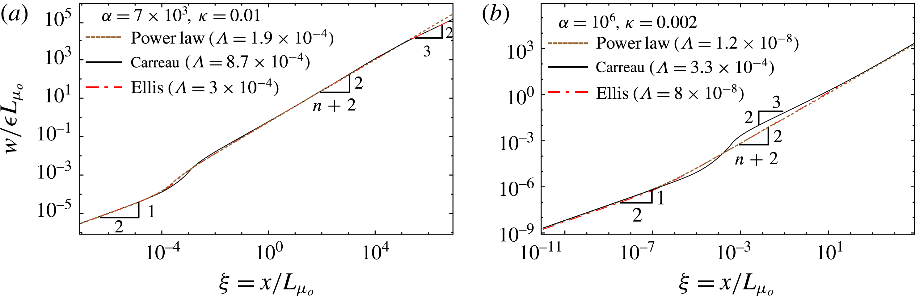
A similar structure for the fracture opening profile is observed for the Ellis and Carreau in figure 12 for the case
 $\unicode[STIX]{x1D6FC}=7\times 10^{3}$
,
 $\unicode[STIX]{x1D705}=0.01$
. The toughness region is larger for the Carreau model compared to the other two models as well as the lag size (Carreau
 $\unicode[STIX]{x1D6EC}=8.7\times 10^{-4}$
, Ellis
 $\unicode[STIX]{x1D6EC}=3\times 10^{-4}$
, and power law
 $\unicode[STIX]{x1D6EC}=1.9\times 10^{-4}$
). As one moves away from the tip (
 $\unicode[STIX]{x1D709}>10^{-2}$
), the Ellis model follows closely the Carreau solution all the way to the far-field zero shear rate viscosity asymptote
 $m_{o}$
(slope in
 $2/3$
). Similarly, the power-law model also follows closely the Carreau solution in the intermediate power-law region but starts to deviate in the far field (
 $\unicode[STIX]{x1D709}>10^{5}$
) where the low shear rate plateau (absent from the power-law model) starts to dominate. For such a value of dimensionless transition shear stress (
 $\unicode[STIX]{x1D6FC}=7\times 10^{3}$
), the tangent apparent viscosity of the Carreau model did not reach the large shear rate Newtonian plateau near the fluid front, and thus the
 $m_{\infty }$
asymptote is not visible in the corresponding Carreau opening profiles.
On the contrary, for
 $\unicode[STIX]{x1D6FC}=10^{6}$
and
 $\unicode[STIX]{x1D705}=0.002$
, the large shear rate asymptote is reached near the fluid front for the Carreau model and the
 $m_{\infty }$
asymptote is clearly visible in the opening profile (figure 12
b). As a result, both the power-law and Ellis models – which do not capture the large shear rate viscosity – are significantly off from the Carreau rheology for that case. This difference observed in the transition between the near-tip toughness asymptote and the far-field shear-thinning regions increases with increasing
 $\unicode[STIX]{x1D6FC}$
. The values of the corresponding dimensionless lag sizes are respectively Carreau
 $\unicode[STIX]{x1D6EC}=3.3\times 10^{-4}$
, Ellis
 $\unicode[STIX]{x1D6EC}=8\times 10^{-8}$
and power law
 $\unicode[STIX]{x1D6EC}=1.2\times 10^{-8}$
. The power-law and Ellis models actually always underestimate the value of the fluid lag for any value of dimensionless shear stress and toughness. This is due to their over-estimation of the shear-thinning behaviour over the complete range of shear rates.
Dimensionless fracture opening
 $w/\unicode[STIX]{x1D716}L_{\unicode[STIX]{x1D707}_{o}}$
along the fracture in log–log scale for Carreau (with
 $\unicode[STIX]{x1D707}_{\infty }/\unicode[STIX]{x1D707}_{o}=10^{-3}$
), Ellis, power-law rheology: (a)
 $\unicode[STIX]{x1D6FC}=7\times 10^{3}$
(
 $\unicode[STIX]{x1D6FC}_{e}=4975$
, Ellis model),
 $n=0.46$
and
 $\unicode[STIX]{x1D705}=0.01$
, (b)
 $\unicode[STIX]{x1D6FC}=10^{6}$
(
 $\unicode[STIX]{x1D6FC}_{e}=7.2\times 10^{5},$
Ellis model),
 $n=0.46$
and
 $\unicode[STIX]{x1D705}=0.002$
.

7 Case of a vanishing fluid lag/large dimensionless toughness (
$\unicode[STIX]{x1D6EC}\approx 0/\unicode[STIX]{x1D705}\gg 1$
)

7.1 Scaling
The limiting case of large dimensionless toughness
 $\unicode[STIX]{x1D705}\gg 1$
corresponds to a vanishing lag. As can be observed from (3.5), large confining stress
 $\unicode[STIX]{x1D70E}_{o}$
implies large dimensionless toughness. A situation that will necessarily occur at great depth in the sub-surface
 $(\unicode[STIX]{x1D70E}_{o}>1~\text{MPa})$
. The limit of zero lag is therefore particularly important in hydraulic fracturing practice. Moreover, as observed previously, the effect of the fluid lag is localized near the tip region and does not readily influence the transition between the different viscosities power-law asymptotic regions (see figure 7 for example). We will therefore analyse in more depth the influence of the different governing parameters on the extent of these different asymptotic regions on the zero-lag case.
The zero-lag assumption leads to the disappearance of the pressure boundary condition
 $p=\unicode[STIX]{x1D70E}_{o}$
and the net pressure becomes singular at the fracture tip (see Garagash & Detournay (Reference Garagash and Detournay2000), Garagash et al. (Reference Garagash, Detournay and Adachi2011) for discussion on the Newtonian case). As a result, another scaling – following Garagash et al. (Reference Garagash, Detournay and Adachi2011) – has to be adopted (see appendix D). We can choose for example to scale the width, net pressure and distance from the tip using the scaling for the transition between the toughness and low shear rate viscosity asymptote. We therefore use a new characteristic opening
 $w_{m_{o}k}$
, pressure
 $p_{m_{o}k}$
and length
 $\ell _{m_{o}k}$
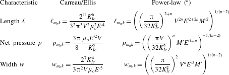
(see table 2) and express the solution as:
 $$\begin{eqnarray}w=w_{m_{o}k}\bar{\unicode[STIX]{x1D6FA}},\quad p=p_{m_{o}k}\bar{\unicode[STIX]{x1D6F1}},\quad x=\ell _{m_{o}k}\bar{\unicode[STIX]{x1D709}},\end{eqnarray}$$
where
 $\bar{\unicode[STIX]{x1D6FA}}$
,
 $\bar{\unicode[STIX]{x1D6F1}}$
and
 $\bar{\unicode[STIX]{x1D709}}$
are the dimensionless width, net pressure and spatial coordinates. The length scale
 $\ell _{m_{o}k}$
characterizes the transition from the toughness dominated regime to the
 $m_{o}$
viscosity regime. It is defined as the distance
 $x$
from the tip where the toughness asymptote and the low shear rate viscosity asymptote intersect:
 $w\sim \ell _{k}^{1/2}x^{1/2}\sim \ell _{m_{o}}^{1/3}x^{2/3}$
(see § 4 for the expression of the different asymptotes). Similarly
 $w_{m_{o}k}$
and
 $p_{m_{o}k}$
are the corresponding characteristic pressure and width where these two asymptotes intersect.
Characteristic scales for the zero-lag case for the three different rheology. The low shear rate viscosity Newtonian scaling is used for both the Ellis and Carreau model.
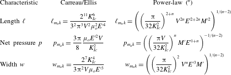
In such a zero-lag scaling, the solution of the problem depends now on three remaining dimensionless parameters: the fluid index
 $n$
, dimensionless transition shear stress and the extent of the shear-thinning magnitude
 $\unicode[STIX]{x1D707}_{\infty }/\unicode[STIX]{x1D707}_{o}$
. The dimensionless transition shear stress is now defined slightly differently due to the different definition of the characteristic length scale and pressure for this zero-lag case. We obtain (see appendix D for more details):
 $$\begin{eqnarray}\bar{\unicode[STIX]{x1D6FC}}=\left(\frac{3\unicode[STIX]{x03C0}}{8}\right)^{2}\frac{\unicode[STIX]{x1D707}_{o}E^{\prime 3}V^{2}}{\dot{\unicode[STIX]{x1D6FE}}_{c}K_{Ic}^{4}}.\end{eqnarray}$$
The value of this dimensionless transition shear stress varies significantly depending on both fluid and rock properties. It may actually span an interval as wide as
 $\bar{\unicode[STIX]{x1D6FC}}\in [10,10^{7}]$
, taking values for shear-thinning fluid (see table 1) and typical ranges of rock properties.
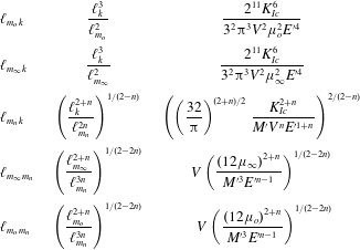
Transition length scales between the different asymptotic regions expressed as a function of the asymptotes characteristic scales (4.1) and directly as function of the problem parameters.

The general solution follows the same structure as in the non-zero-lag case. In the region near the fracture tip, the fracture toughness is the dominating dissipative process and govern the fracture width. As we move away from the tip, the dissipation in the fluid takes over as the dominant mechanism. Depending on the dimensionless transition shear stress
 $\bar{\unicode[STIX]{x1D6FC}}$
, fluid index
 $n$
and extent of the shear thinning
 $\unicode[STIX]{x1D707}_{\infty }/\unicode[STIX]{x1D707}_{o}$
, three different viscosity asymptotic regions can be observed: high shear rate viscosity asymptote
 $m_{\infty }$
for large values of the wall shear stress when the low shear rate Newtonian viscosity plateau
 $\dot{\unicode[STIX]{x1D6FE}}_{c}$
is small enough (large
 $\bar{\unicode[STIX]{x1D6FC}}$
), power-law viscosity asymptote
 $m_{n}$
in an intermediate shear-thinning region and the low shear rate viscosity asymptote
 $m_{o}$
for small values of shear rate/large distances from the tip.
The extent, occurrence and transition between these asymptotic regions can be estimated based on the different limiting asymptotes (see § 4), by defining transition length scales where two given asymptotes intersect. For example, one can define
 $\ell _{m_{\infty }k}$
as the transition length scale between the
 $k$
-asymptote to the
 $m_{\infty }$
-asymptote as the distance
 $x$
from the tip where the two asymptotes are comparable:
 $w\sim \ell _{k}^{1/2}x^{1/2}\sim \ell _{m_{\infty }}^{1/3}x^{2/3}$
such that we obtain
 $x=\ell _{m_{\infty }k}=\ell _{k}^{3}/\ell _{m_{\infty }}^{2}$
. We can also define a transition length scale between the toughness
 $k$
and power-law
 $m_{n}$
asymptotes, the distance
 $x$
where
 $w\sim \ell _{k}^{1/2}x^{1/2}\sim \ell _{m_{n}}^{n/(2+n)}x^{2/(n+2)}$
, i.e.
 $x=\ell _{m_{n}k}=(\ell _{k}^{2+n}/\ell _{m_{n}}^{2n})^{1/(2-n)}$
. Similarly, we can define
 $\ell _{m_{\infty }m_{n}}$
and
 $\ell _{m_{o}m_{n}}$
as the boundaries of the high shear rate power-law viscosity and low shear rate viscosity power-law asymptotic regions. The expressions of these different transition length scales can be found in table 3 as function of the problem parameters as well as function of the length scales
 $\ell _{k}$
,
 $\ell _{m_{\infty }}$
,
 $\ell _{m_{n}}$
and
 $\ell _{m_{o}}$
.
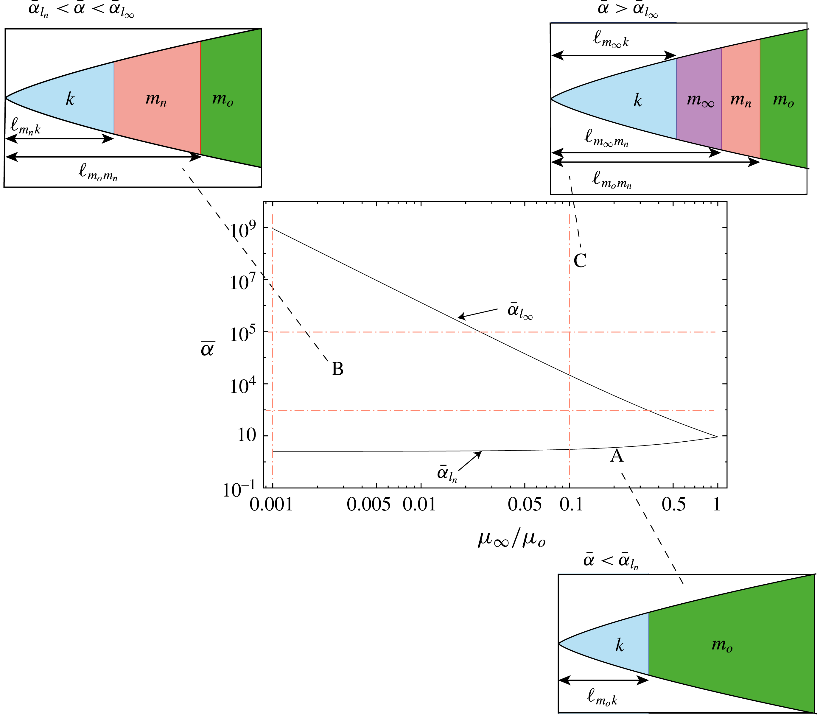
Occurrence of the different viscous asymptotes as a function of
 $\bar{\unicode[STIX]{x1D6FC}}$
and
 $\unicode[STIX]{x1D707}_{\infty }/\unicode[STIX]{x1D707}_{o}$
for
 $n=0.46$
. Three distinct regions separate the parametric space: region A defined as
 $\bar{\unicode[STIX]{x1D6FC}}<\bar{\unicode[STIX]{x1D6FC}}_{l_{n}}(\unicode[STIX]{x1D707}_{\infty }/\unicode[STIX]{x1D707}_{o},n)$
where the solution transitions from
 $k$
directly to
 $m_{o}$
, region B defined as
 $\bar{\unicode[STIX]{x1D6FC}}_{l_{n}}(\unicode[STIX]{x1D707}_{\infty }/\unicode[STIX]{x1D707}_{o},n)<\bar{\unicode[STIX]{x1D6FC}}<\bar{\unicode[STIX]{x1D6FC}}_{l_{\infty }}(\unicode[STIX]{x1D707}_{\infty }/\unicode[STIX]{x1D707}_{o},n)$
where three asymptotes
 $k$
,
 $m_{n}$
and
 $m_{o}$
can be observed and region C defined for
 $\bar{\unicode[STIX]{x1D6FC}}>\bar{\unicode[STIX]{x1D6FC}}_{l_{\infty }}(\unicode[STIX]{x1D707}_{\infty }/\unicode[STIX]{x1D707}_{o},n)$
where up to four asymptotes
 $k$
,
 $m_{\infty }$
,
 $m_{n}$
and
 $m_{o}$
may be observed. The dot-dashed orange lines refer to the coordinates of the numerical simulations performed in figure 14.

It is important to realize that depending on the dimensionless transition shear stress
 $\bar{\unicode[STIX]{x1D6FC}}$
, shear-thinning index
 $n$
and extent
 $\unicode[STIX]{x1D707}_{\infty }/\unicode[STIX]{x1D707}_{o}$
, not all of the different asymptotes may be realized in the solution. For example, the high shear rate viscosity regime can only be seen if the solution transitions first from the toughness
 $k$
asymptote to the
 $m_{\infty }$
and then
 $m_{n}$
asymptotes. In other words, if the
 $m_{n}k$
transition length scale is larger than the
 $m_{\infty }k$
transition length scale:
 $\ell _{m_{n}k}>\ell _{m_{\infty }k}$
. This condition
 $\ell _{m_{n}k}>\ell _{m_{\infty }k}$
can be re-expressed as the boundary of a region in the parametric space
 $n-\bar{\unicode[STIX]{x1D6FC}}-\unicode[STIX]{x1D707}_{\infty }/\unicode[STIX]{x1D707}_{o}$
. For a given
 $n$
, this region can be seen in figure 13, and expressed in terms of a limiting transition shear stress
 $\bar{\unicode[STIX]{x1D6FC}}_{l_{\infty }}(\unicode[STIX]{x1D707}_{\infty }/\unicode[STIX]{x1D707}_{o},n)$
(
 $\bar{\unicode[STIX]{x1D6FC}}_{l_{\infty }}$
is a decreasing function of
 $\unicode[STIX]{x1D707}_{\infty }/\unicode[STIX]{x1D707}_{o}$
). For
 $\bar{\unicode[STIX]{x1D6FC}}>\bar{\unicode[STIX]{x1D6FC}}_{l_{\infty }}(\unicode[STIX]{x1D707}_{\infty }/\unicode[STIX]{x1D707}_{o},n)$
, the solution exhibits all the possible asymptotes:
 $k$
,
 $m_{\infty }$
,
 $m_{n}$
and
 $m_{o}$
as one moves away from the fracture tip. This limit can be obtained from the equality
 $\ell _{m_{n}k}=\ell _{m_{\infty }k}$
and can actually be expressed analytically as function of
 $n$
and
 $\unicode[STIX]{x1D707}_{\infty }/\unicode[STIX]{x1D707}_{o}$
:
 $$\begin{eqnarray}\bar{\unicode[STIX]{x1D6FC}}_{l_{\infty }}=\frac{\sqrt{2^{-2/(n-1)}-1}}{\left({\displaystyle \frac{6n}{1+2n}}\right)^{n/(1-n)}}\left(\frac{\left(\unicode[STIX]{x1D707}_{\infty }/\unicode[STIX]{x1D707}_{o}\right)^{^{2-n}}}{1+\unicode[STIX]{x1D707}_{\infty }/\unicode[STIX]{x1D707}_{o}}\right)^{1/(n-1)}.\end{eqnarray}$$
Another case worth considering is when
 $\ell _{m_{n}k}>\ell _{m_{o}m_{n}}$
. This means that the distance at which the solution transition from the power-law to the low shear rate viscosity is smaller than the distance at which the solution transition from the toughness to the power-law region. In other words, because the shear rate decreases as one moves away from the tip, such a situation indicates that no power-law asymptotic region exists. The condition
 $\ell _{m_{n}k}=\ell _{m_{o}m_{n}}$
therefore defines another boundary of a region in the parametric space where the solution exhibits only two asymptotic regions: the toughness
 $k$
asymptote near the tip and the low shear rate viscosity
 $m_{o}$
away from the tip. Similarly, for a given
 $n$
, this boundary can be recast in terms of a limiting value of the dimensionless transition shear stress
 $\bar{\unicode[STIX]{x1D6FC}}_{l_{n}}(\unicode[STIX]{x1D707}_{\infty }/\unicode[STIX]{x1D707}_{o},n)$
expressed as function of
 $n$
and
 $\unicode[STIX]{x1D707}_{\infty }/\unicode[STIX]{x1D707}_{o}$
(
 $\bar{\unicode[STIX]{x1D6FC}}_{l_{n}}$
increases with
 $\unicode[STIX]{x1D707}_{\infty }/\unicode[STIX]{x1D707}_{o}$
):
 $$\begin{eqnarray}\bar{\unicode[STIX]{x1D6FC}}_{l_{n}}=\frac{\sqrt{2^{-2/(n-1)}-1}}{\left({\displaystyle \frac{6n}{1+2n}}\right)^{n/(1-n)}}\left(\frac{1}{1+\unicode[STIX]{x1D707}_{\infty }/\unicode[STIX]{x1D707}_{o}}\right)^{1/(n-1)}.\end{eqnarray}$$
The two limits are actually related as
 $$\begin{eqnarray}\bar{\unicode[STIX]{x1D6FC}}_{l\infty }=\bar{\unicode[STIX]{x1D6FC}}_{l_{n}}\times \left(\frac{\unicode[STIX]{x1D707}_{\infty }}{\unicode[STIX]{x1D707}_{o}}\right)^{-(2+n)/(1-n)}.\end{eqnarray}$$
Figure 13 displays these two limits for
 $n=0.46$
which therefore define three regions in the parametric space. In region A (
 $\bar{\unicode[STIX]{x1D6FC}}<\bar{\unicode[STIX]{x1D6FC}}_{l_{n}}(\unicode[STIX]{x1D707}_{\infty }/\unicode[STIX]{x1D707}_{o})$
), only two asymptotic regions (
 $k$
and
 $m_{o}$
) are present in the solution. In region B, for
 $\bar{\unicode[STIX]{x1D6FC}}_{l_{n}}(\unicode[STIX]{x1D707}_{\infty }/\unicode[STIX]{x1D707}_{o})<\bar{\unicode[STIX]{x1D6FC}}<\bar{\unicode[STIX]{x1D6FC}}_{l_{\infty }}(\unicode[STIX]{x1D707}_{\infty }/\unicode[STIX]{x1D707}_{o})$
, three asymptotic regions
 $k$
,
 $m_{n}$
and
 $m_{o}$
are present as one moves away from the tip. Finally,
 $\bar{\unicode[STIX]{x1D6FC}}>\bar{\unicode[STIX]{x1D6FC}}_{l_{\infty }}(\unicode[STIX]{x1D707}_{\infty }/\unicode[STIX]{x1D707}_{o})$
defines a third region where all the different asymptotes may be visible:
 $k$
,
 $m_{\infty }$
,
 $m_{n}$
and
 $m_{o}$
in that order from the tip.
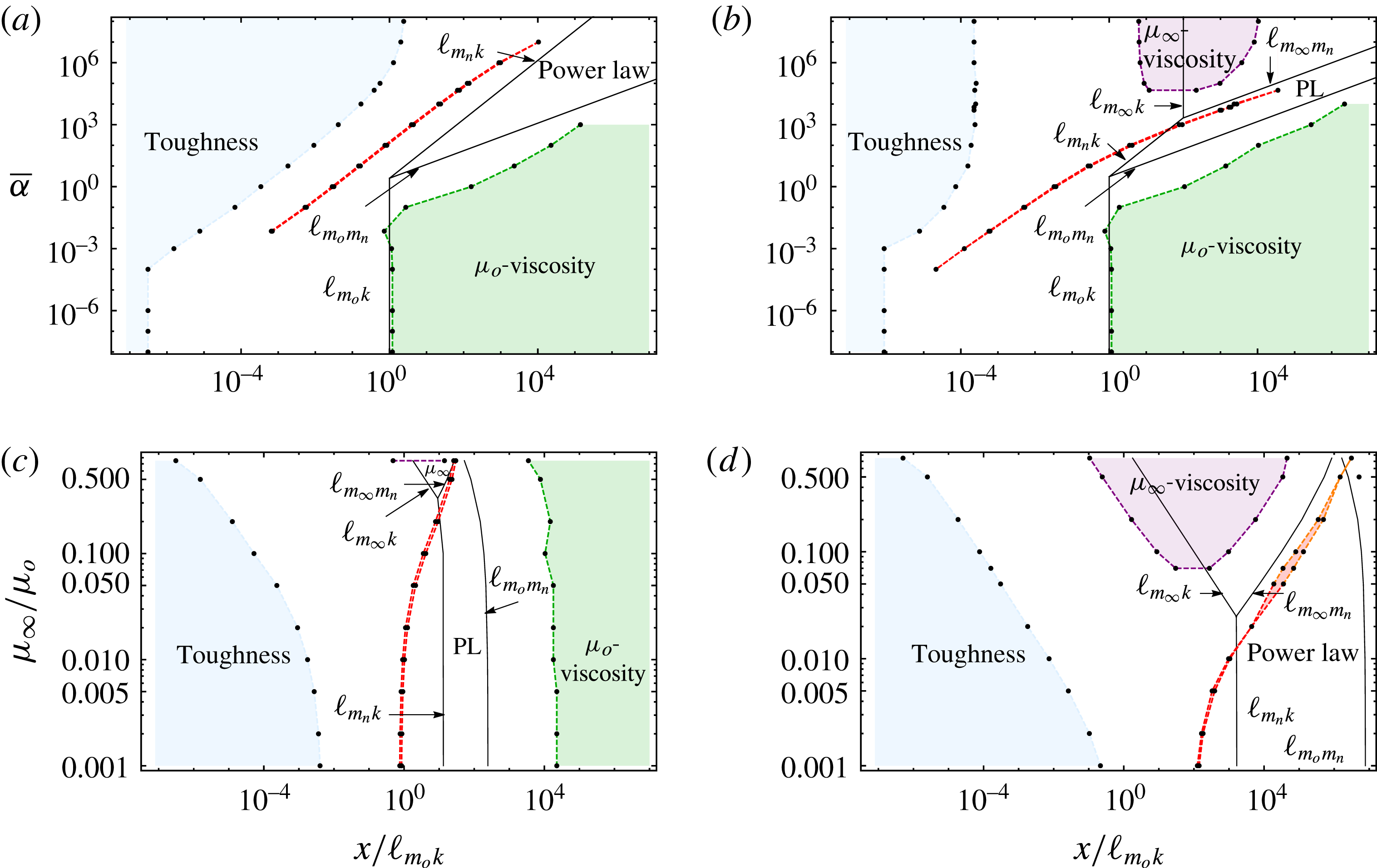
Numerical bounds and transition length scales (black solid lines) between the different asymptotic regions: (a) variations of
 $\bar{\unicode[STIX]{x1D6FC}}$
for
 $n=0.46,$
 $\unicode[STIX]{x1D707}_{\infty }/\unicode[STIX]{x1D707}_{o}=10^{-3}$
, (b) variations of
 $\bar{\unicode[STIX]{x1D6FC}}$
for
 $n=0.46,$
 $\unicode[STIX]{x1D707}_{\infty }/\unicode[STIX]{x1D707}_{o}=10^{-1}$
, (c) variations of
 $\unicode[STIX]{x1D707}_{\infty }/\unicode[STIX]{x1D707}_{o}$
for
 $n=0.46,$
 $\bar{\unicode[STIX]{x1D6FC}}=10^{2}$
and (d)
 $\unicode[STIX]{x1D707}_{\infty }/\unicode[STIX]{x1D707}_{o}$
for
 $n=0.46,$
 $\bar{\unicode[STIX]{x1D6FC}}=10^{5}$
. The regions where the numerical results fall within
 $1\,\%$
of accuracy of an asymptote are also displayed. For the power-law region, limits where the numerical results are within
 $1\,\%$
accuracy of the
 $m_{n}$
asymptote are displayed in red, and in orange when within
 $5\,\%$
of accuracy.

7.2 Evolution of the different asymptotic regions
In the previous section, based on scaling considerations, we have defined three distinct regions in the parametric space, where two, three or four asymptotic regions may be observed. Here we compare a large series of numerical results (57 simulations in total) with the limits established previously. We plot as function of the scaled distance from the tip
 $x/\ell _{m_{o}k}$
the limits where the numerical results are within 1 % of the different asymptotes as function of
 $\bar{\unicode[STIX]{x1D6FC}}$
(for a given
 $n$
and
 $\unicode[STIX]{x1D707}_{\infty }/\unicode[STIX]{x1D707}_{o}$
) or
 $\unicode[STIX]{x1D707}_{\infty }/\unicode[STIX]{x1D707}_{o}$
(for a given
 $n$
and
 $\bar{\unicode[STIX]{x1D6FC}}$
). For comparison, we also plot the analytical asymptotic transitions based on the defined length scales (table 3).
We perform four series of simulations corresponding to two vertical and two horizontal cross-sections of the parametric space
 $\bar{\unicode[STIX]{x1D6FC}}-\unicode[STIX]{x1D707}_{\infty }/\unicode[STIX]{x1D707}_{o}$
(see figure 13). All reported simulations are for
 $n=0.46$
(HPG fluid index). The value of
 $n$
modifies the shape of the different boundaries but does not change qualitatively the overall picture. The results of these four series of simulations are summarized in figure 14.
Let us first discuss the cases where we vary
 $\bar{\unicode[STIX]{x1D6FC}}$
in the range
 $[10^{-8},10^{8}]$
for two distinct values of the shear-thinning magnitude
 $\unicode[STIX]{x1D707}_{\infty }/\unicode[STIX]{x1D707}_{o}=10^{-3}$
and
 $\unicode[STIX]{x1D707}_{\infty }/\unicode[STIX]{x1D707}_{o}=10^{-1}$
(top plots in figure 14). The overall extent of the different asymptotic regions as a function of tip distance and dimensionless transition shear stress follow the structure presented previously. For small value of
 $\bar{\unicode[STIX]{x1D6FC}}$
, only the toughness (near the tip) and low shear rate viscosity
 $m_{o}$
asymptotes are visible. Above a given value of
 $\bar{\unicode[STIX]{x1D6FC}}$
, the power-law asymptote starts to be visible in our numerical results albeit in a very narrow region (for a relative asymptotic error of
 $1\%$
). Finally, for large
 $\bar{\unicode[STIX]{x1D6FC}}$
for
 $\unicode[STIX]{x1D707}_{\infty }/\unicode[STIX]{x1D707}_{o}=10^{-1}$
, the large shear rate viscosity
 $m_{\infty }$
asymptote can be clearly seen in the numerical results. For these two series of simulations for
 $\unicode[STIX]{x1D707}_{\infty }/\unicode[STIX]{x1D707}_{o}=10^{-3}$
and
 $10^{-1}$
, the limiting values
 $\bar{\unicode[STIX]{x1D6FC}}_{l_{n}}$
under which only the toughness and low shear rate viscosity asymptotes are present are respectively
 $\bar{\unicode[STIX]{x1D6FC}}_{l_{n}}(\unicode[STIX]{x1D707}_{\infty }/\unicode[STIX]{x1D707}_{o}=10^{-1})=3.03$
, and
 $\bar{\unicode[STIX]{x1D6FC}}_{l_{n}}(\unicode[STIX]{x1D707}_{\infty }/\unicode[STIX]{x1D707}_{o}=10^{-3})=2.55$
. Our numerical results report a smaller value for this lower limit
 $\bar{\unicode[STIX]{x1D6FC}}_{l_{n}}$
:
 $\bar{\unicode[STIX]{x1D6FC}}_{l_{n_{num}}}(\unicode[STIX]{x1D707}_{\infty }/\unicode[STIX]{x1D707}_{o}=10^{-1})\simeq 10^{-4}$
and
 $\bar{\unicode[STIX]{x1D6FC}}_{l_{n_{num}}}(\unicode[STIX]{x1D707}_{\infty }/\unicode[STIX]{x1D707}_{o}=10^{-3})\simeq 10^{-2}$
. For the small shear-thinning magnitude case (
 $\unicode[STIX]{x1D707}_{\infty }/\unicode[STIX]{x1D707}_{o}=10^{-1}$
), the high shear rate viscosity region is visible in figure 14(b) for values of
 $\bar{\unicode[STIX]{x1D6FC}}$
greater than
 $\bar{\unicode[STIX]{x1D6FC}}_{l_{\infty }}(\unicode[STIX]{x1D707}_{\infty }/\unicode[STIX]{x1D707}_{o}=10^{-1})=2.1\times 10^{4}$
, while the numerical value at which we start to observe the
 $m_{\infty }$
asymptote is slightly larger
 $\bar{\unicode[STIX]{x1D6FC}}_{l_{\infty _{num}}}(\unicode[STIX]{x1D707}_{\infty }/\unicode[STIX]{x1D707}_{o}=10^{-1})\simeq 4.6\times 10^{4}$
. Note that for
 $\unicode[STIX]{x1D707}_{\infty }/\unicode[STIX]{x1D707}_{o}=10^{-3}$
, the high shear rate viscosity region is pushed out of the dimensionless transition shear stress interval investigated here, the analytical expression gives
 $\bar{\unicode[STIX]{x1D6FC}}_{l_{\infty }}(\unicode[STIX]{x1D707}_{\infty }/\unicode[STIX]{x1D707}_{o}=10^{-3})=9.1\times 10^{8}$
in that case, and the
 $m_{\infty }$
asymptote is not visible on our numerical results.
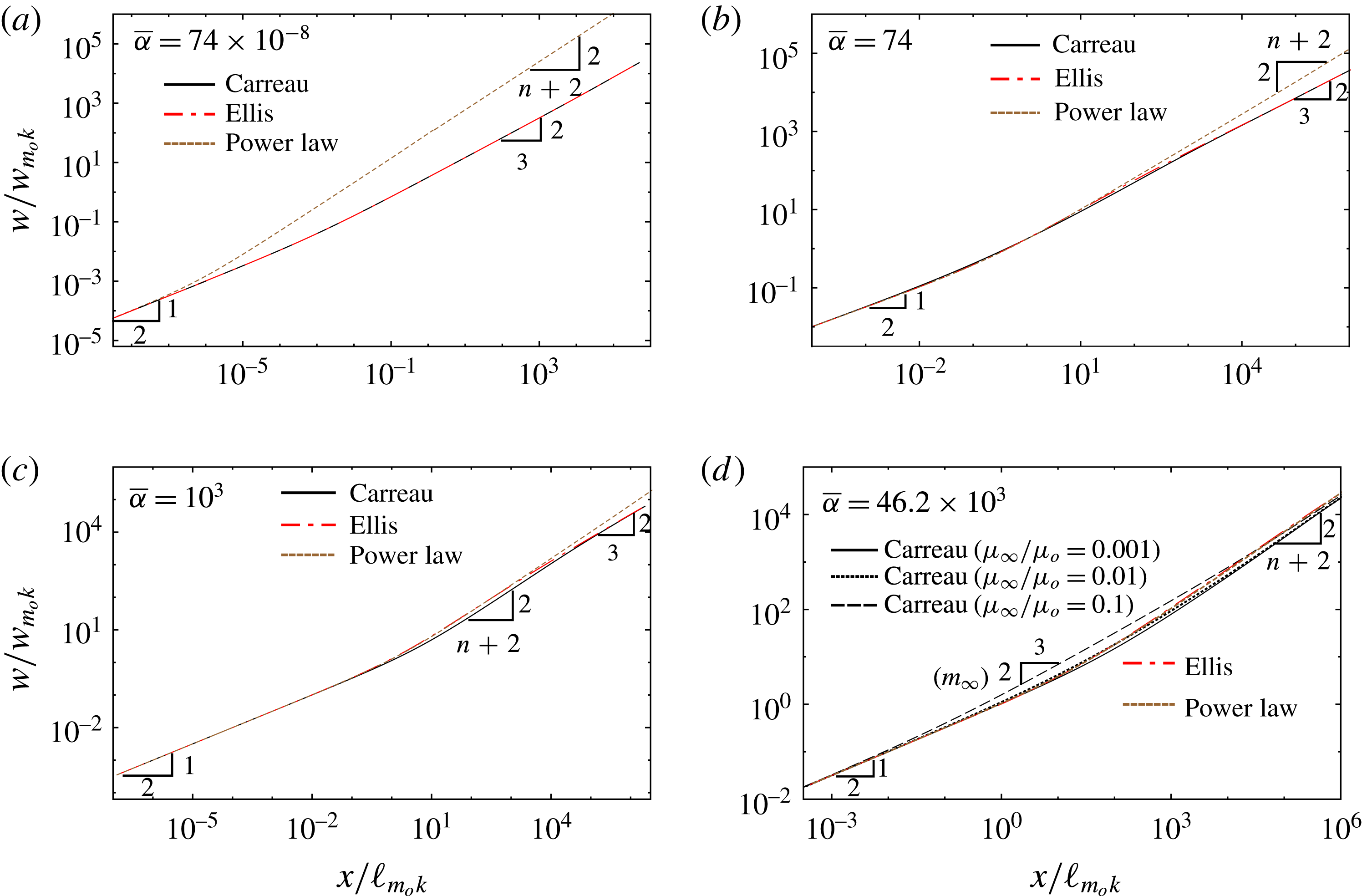
Zero-lag case. Dimensionless fracture opening
 $w/w_{m_{o}k}$
as a function of the dimensionless distance from the tip
 $x/\ell _{m_{o}k}$
for the three rheologies (see table 2 for the expressions of the characteristic scales
 $w_{m_{o}k}$
and
 $\ell _{m_{o}k}$
). The rheological parameters of the fluid are those of HPG. Influence of
 $\bar{\unicode[STIX]{x1D6FC}}$
with
 $\unicode[STIX]{x1D707}_{\infty }/\unicode[STIX]{x1D707}_{o}=10^{-3}$
: (a)
 $\bar{\unicode[STIX]{x1D6FC}}=74\times 10^{-8}$
(Ellis
 $\bar{\unicode[STIX]{x1D6FC}}_{e}=53.4\times 10^{-8}$
), (b)
 $\bar{\unicode[STIX]{x1D6FC}}=74$
(Ellis
 $\bar{\unicode[STIX]{x1D6FC}}_{e}=53.4$
; (c)
 $\bar{\unicode[STIX]{x1D6FC}}=10^{3}$
(Ellis
 $\bar{\unicode[STIX]{x1D6FC}}_{e}=2088.7$
), (d)
 $\bar{\unicode[STIX]{x1D6FC}}=46.2\times 10^{3}$
(Ellis
 $\bar{\unicode[STIX]{x1D6FC}}_{e}=33.4\times 10^{3}$
) with also the solution for different
 $\unicode[STIX]{x1D707}_{\infty }/\unicode[STIX]{x1D707}_{o}$
for the Carreau model. The Ellis model starts to depart from the Carreau in the intermediate region for
 $\unicode[STIX]{x1D6FC}\geqslant 10^{3}$
even for a large shear-thinning magnitude (
 $\unicode[STIX]{x1D707}_{\infty }/\unicode[STIX]{x1D707}_{o}=10^{-3}$
).

The extent of the toughness region near the fracture tip is roughly constant for small
 $\bar{\unicode[STIX]{x1D6FC}}$
, then increases with
 $\bar{\unicode[STIX]{x1D6FC}}$
until reaching a constant value for sufficiently large
 $\bar{\unicode[STIX]{x1D6FC}}$
(above the limit
 $\bar{\unicode[STIX]{x1D6FC}}_{l_{\infty }}$
) for which the
 $m_{\infty }$
asymptote becomes visible. For small enough values of
 $\bar{\unicode[STIX]{x1D6FC}}$
(below
 $\bar{\unicode[STIX]{x1D6FC}}_{l_{n}}$
), the distance at which the numerical results can be approximated by the toughness and low shear rate viscosity asymptote are respectively
 $x\approx 10^{-7}\ell _{m_{o}k}$
and
 $x\approx 1.3\ell _{m_{o}k}$
which are consistent with the bounds obtained by Garagash et al. (Reference Garagash, Detournay and Adachi2011). Similarly, for the case of large dimensionless transition shear stress
 $\bar{\unicode[STIX]{x1D6FC}}>\bar{\unicode[STIX]{x1D6FC}}_{l_{\infty }}$
, the numerical boundaries demonstrate that the
 $m_{\infty }$
asymptote starts at
 $x\approx 10^{1}\ell _{m_{o}k}$
from the fracture tip regardless the value of
 $\bar{\unicode[STIX]{x1D6FC}}$
.
Similarly we have studied the effect of the viscosity ratio in the range
 $[10^{-3},0.75]$
for two distinct dimensionless transition shear stress
 $\bar{\unicode[STIX]{x1D6FC}}=10^{2}$
and
 $10^{5}$
, see figure 14(c,d). In both cases, the extent of the toughness region (scaled by
 $\ell _{m_{o}k}$
) is decreasing with larger values of
 $\unicode[STIX]{x1D707}_{\infty }/\unicode[STIX]{x1D707}_{o}$
. In fact, the evolution of the toughness region tracks the evolution of
 $\ell _{m_{n}k}$
and
 $\ell _{m_{\infty }k}$
as a function of
 $\bar{\unicode[STIX]{x1D6FC}}$
and
 $\unicode[STIX]{x1D707}_{\infty }/\unicode[STIX]{x1D707}_{o}$
for all cases.
For the series of simulation with
 $\bar{\unicode[STIX]{x1D6FC}}=10^{2}$
, the
 $m_{o}$
low shear rate viscosity region has the same domain of validity regardless of the value of
 $\unicode[STIX]{x1D707}_{\infty }/\unicode[STIX]{x1D707}_{o}$
(figure 14
c). This low shear rate region cannot, however, be observed for the series of simulation with
 $\bar{\unicode[STIX]{x1D6FC}}=10^{5}$
, where it is estimated to appear for distances away from the tip above
 $10^{7}\ell _{m_{o}k}$
. A value which is larger than the extent of our computational domain.
The high shear rate viscosity region
 $m_{\infty }$
can be seen for values of
 $\unicode[STIX]{x1D707}_{\infty }/\unicode[STIX]{x1D707}_{o}$
larger than
 $0.33$
(
 $\bar{\unicode[STIX]{x1D6FC}}=10^{2}$
) and
 $0.025$
(
 $\bar{\unicode[STIX]{x1D6FC}}=10^{5}$
) respectively from the scaling arguments. These values are in line with the numerical results which gives respectively
 $(\unicode[STIX]{x1D707}_{\infty }/\unicode[STIX]{x1D707}_{o})_{num}=0.75$
(
 $\bar{\unicode[STIX]{x1D6FC}}=10^{2}$
, where this
 $m_{\infty }$
region can be seen for the largest value of
 $\unicode[STIX]{x1D707}_{\infty }/\unicode[STIX]{x1D707}_{o}$
only), and
 $(\unicode[STIX]{x1D707}_{\infty }/\unicode[STIX]{x1D707}_{o})_{num}=0.07$
(
 $\bar{\unicode[STIX]{x1D6FC}}=10^{5}$
).
It is also worthwhile to note that for all the simulations reported in figure 14, the extent of the power-law region where the numerical results obtained are within
 $1\%$
of the
 $m_{n}$
asymptote is extremely limited, and significantly smaller than the predictions obtained from scaling arguments.
7.3 Comparison between the Carreau, power-law and Ellis models
In this section, we compare these three models in the zero-lag case and investigate how close the predictions based on Ellis and power-law models are to the complete Carreau model depending on the occurrence of the different asymptotic regions highlighted in figure 13. We use the zero-lag scaling (7.1) in all cases. The expressions of the characteristic opening, pressure and length for the power-law model (see table 2) are different from the Carreau model (while they are similar for the Ellis model). The scaling and dimensionless problem are detailed in appendix D.
Like previously for the lag case, we fix the rheological parameters to the ones reproducing the rheology of an HPG fluid (see table 1 for the different models). We vary the value of the dimensionless transition shear stress
 $\bar{\unicode[STIX]{x1D6FC}}$
(by varying
 $E^{\prime 3}V^{2}/K_{Ic}^{4}$
at fix rheological parameters), as well as the shear-thinning amplitude ratio
 $\unicode[STIX]{x1D707}_{\infty }/\unicode[STIX]{x1D707}_{o}$
.
We first fix the shear-thinning magnitude
 $\unicode[STIX]{x1D707}_{\infty }/\unicode[STIX]{x1D707}_{o}$
at
 $10^{-3}$
. Figure 15(a–d) exhibits the fracture opening for the three models for four different values of
 $\bar{\unicode[STIX]{x1D6FC}}$
(small
 $\bar{\unicode[STIX]{x1D6FC}}$
– figure 15(a), intermediate
 $\bar{\unicode[STIX]{x1D6FC}}$
– figure 15(b,c) and large
 $\bar{\unicode[STIX]{x1D6FC}}$
– figure 15
d). As discussed in figure 13, there are two limits that define the behaviour of solution for the Carreau model
 $(\bar{\unicode[STIX]{x1D6FC}}_{l_{n}},\bar{\unicode[STIX]{x1D6FC}}_{l_{\infty }})$
for a given viscosity ratio and power-law index. These values of the dimensionless transition shear stress can be approximated analytically using the transition length scales (see § 7.1). For
 $\unicode[STIX]{x1D707}_{\infty }/\unicode[STIX]{x1D707}_{o}=10^{-3}$
, the high shear rate viscosity asymptote may become visible for values of
 $\bar{\unicode[STIX]{x1D6FC}}$
larger than
 $\bar{\unicode[STIX]{x1D6FC}}_{l_{\infty }}=9.1\times 10^{8}$
, whereas the power-law region may appear for
 $\bar{\unicode[STIX]{x1D6FC}}$
larger than
 $\bar{\unicode[STIX]{x1D6FC}}_{l_{n}}=2.55$
.
For value of
 $\bar{\unicode[STIX]{x1D6FC}}$
smaller than
 $\bar{\unicode[STIX]{x1D6FC}}_{l_{n}}$
(see figure 15
a), as expected the Carreau dimensionless opening transition from the toughness
 $k$
asymptote near the tip to the far-field low shear viscosity asymptote without any visible power-law region. The solution for the Ellis model matches perfectly the solution of the Carreau rheology for that case (figure 15
a). As expected, the prediction of the power-law rheology widely differs from Carreau for this small
 $\bar{\unicode[STIX]{x1D6FC}}$
case (due to the large effect of the low shear rate plateau). As the value of
 $\bar{\unicode[STIX]{x1D6FC}}$
exceeds
 $\bar{\unicode[STIX]{x1D6FC}}_{l_{n}}$
, a power-law region appears just beyond the near-tip toughness region. For
 $\bar{\unicode[STIX]{x1D6FC}}=74$
(see figure 15
b), the Ellis model still follows closely the complete Carreau rheology – excepting a small deviation in the transition between the power-law and far-field regions (for
 $\displaystyle x/\ell _{m_{o}k}\in [1-100]$
). Here again, the power-law model still significantly deviates in the far field due to the effect of the low shear rate viscosity absent from the power-law model. For larger value of
 $\bar{\unicode[STIX]{x1D6FC}}$
(figure 15
c), the difference between the Ellis and Carreau rheology slightly increases in the intermediate power-law
 $m_{n}$
region where the effect of the transition from the power-law branch to the high shear rate Newtonian plateau in the Carreau rheology starts to influence the overall solution (see § 6.2 for details) even tough
 $\bar{\unicode[STIX]{x1D6FC}}$
did not yet reach the bound
 $\bar{\unicode[STIX]{x1D6FC}}_{l_{\infty }}$
. However, the Ellis model still match exactly the Carreau solution in the near-tip toughness region and in the far-field low shear rate
 $m_{o}$
region. The power-law model gets closer to the predictions of the Carreau and the Ellis models except in the far-field low shear rate
 $m_{o}$
region (
 $x/\ell _{m_{o}k}>10^{4}$
) as expected.
All the results depicted in figure 15(a–c) are for the case of a large shear-thinning amplitude (
 $\unicode[STIX]{x1D707}_{\infty }/\unicode[STIX]{x1D707}_{o}=10^{-3}$
). The effect of its influence can be seen in figure 15(d) for a large value of
 $\bar{\unicode[STIX]{x1D6FC}}$
(
 $46.2\times 10^{3}$
). For such a large value of
 $\bar{\unicode[STIX]{x1D6FC}}$
, the power-law region stretches out far away from the tip, actually driving the low shear rate region outside of our numerical grid. Over those length scales, the Ellis and the power-law models are very close to one another. They both differ however from the Carreau rheology outside the near-tip toughness
 $k$
region. Such a difference increases as the shear-thinning amplitude decreases (i.e. for smaller viscosity ratio
 $\unicode[STIX]{x1D707}_{\infty }/\unicode[STIX]{x1D707}_{o}$
). The power-law region significantly decreases in the Carreau solution with increasing viscosity ratio
 $\unicode[STIX]{x1D707}_{\infty }/\unicode[STIX]{x1D707}_{o}$
. The high shear rate viscosity region
 $m_{\infty }$
dominates the Carreau response in the intermediate field for the case
 $\unicode[STIX]{x1D707}_{\infty }/\unicode[STIX]{x1D707}_{o}=10^{-1}$
for
 $\bar{\unicode[STIX]{x1D6FC}}>\bar{\unicode[STIX]{x1D6FC}}_{l_{\infty }}(\unicode[STIX]{x1D707}_{\infty }/\unicode[STIX]{x1D707}_{o}=10^{-1})=2.1\times 10^{4}$
. For both cases
 $\unicode[STIX]{x1D707}_{\infty }/\unicode[STIX]{x1D707}_{o}=10^{-2}$
and
 $\unicode[STIX]{x1D707}_{\infty }/\unicode[STIX]{x1D707}_{o}=10^{-3}$
, the high shear rate viscosity
 $m_{\infty }$
region is still absent from the Carreau solution (
 $\bar{\unicode[STIX]{x1D6FC}}_{l_{n}}(\unicode[STIX]{x1D707}_{\infty }/\unicode[STIX]{x1D707}_{o}=10^{-2})=2.59<\bar{\unicode[STIX]{x1D6FC}}<\bar{\unicode[STIX]{x1D6FC}}_{l_{\infty }}(\unicode[STIX]{x1D707}_{\infty }/\unicode[STIX]{x1D707}_{o}=10^{-2})=1.3\times 10^{6}$
and
 $\bar{\unicode[STIX]{x1D6FC}}<\bar{\unicode[STIX]{x1D6FC}}_{l_{\infty }}(\unicode[STIX]{x1D707}_{\infty }/\unicode[STIX]{x1D707}_{o}=10^{-3})=9.1\times 10^{8}$
) but the solution is already significantly affected by the rather long transition from the power-law branch to the high shear rate viscosity intrinsic to the Carreau model.
These comparisons are in line with the structure of the solution with respect to the different limiting asymptotes depicted in the previous section. We notably see that the scaling estimate of
 $\bar{\unicode[STIX]{x1D6FC}}_{l_{n}}$
and
 $\bar{\unicode[STIX]{x1D6FC}}_{l_{\infty }}$
provides the overall trend of the validity of the different models, with the caveat that the transition from the power-law branch to the high shear rate viscosity plateau has a significant effect on the solution even for
 $\bar{\unicode[STIX]{x1D6FC}}$
lower than
 $\bar{\unicode[STIX]{x1D6FC}}_{l_{\infty }}$
. In summary, for values of
 $\bar{\unicode[STIX]{x1D6FC}}$
sufficiently lower than
 $\bar{\unicode[STIX]{x1D6FC}}_{l_{\infty }}(\unicode[STIX]{x1D707}_{\infty }/\unicode[STIX]{x1D707}_{o},n)$
, the Ellis model reproduces relatively well the results obtained with the Carreau rheology. Deviations start to occur for larger values of the dimensionless shear stress
 $\bar{\unicode[STIX]{x1D6FC}}$
. The power-law model reproduces poorly the results of the complete Carreau solution in the far-field region in all cases. It may only provide an acceptable approximation up to a distance
 $x/\ell _{m_{o}k}\approx 10$
from the tip for intermediate values of
 $\bar{\unicode[STIX]{x1D6FC}}$
in between the limits
 $\bar{\unicode[STIX]{x1D6FC}}_{l_{n}}(\unicode[STIX]{x1D707}_{\infty }/\unicode[STIX]{x1D707}_{o},n)$
and
 $\bar{\unicode[STIX]{x1D6FC}}_{l_{\infty }}(\unicode[STIX]{x1D707}_{\infty }/\unicode[STIX]{x1D707}_{o},n)$
. This intermediate region between
 $\bar{\unicode[STIX]{x1D6FC}}_{l_{n}}(\unicode[STIX]{x1D707}_{\infty }/\unicode[STIX]{x1D707}_{o},n)$
and
 $\bar{\unicode[STIX]{x1D6FC}}_{l_{\infty }}(\unicode[STIX]{x1D707}_{\infty }/\unicode[STIX]{x1D707}_{o},n)$
drastically shrinks for increasing
 $\unicode[STIX]{x1D707}_{\infty }/\unicode[STIX]{x1D707}_{o}$
ratio (i.e. decreasing shear-thinning amplitude).
8 Conclusions
The use of shear-thinning fluids is ubiquitous in hydraulic fracturing applications. By focusing on the near-tip behaviour, we have clarified the impact of the details of the fluid rheological behaviour on the complex coupling between lubrication flow and linear elastic fracture mechanics. Depending on the problem parameters, three scenarios are possible. First (region A in figure 13), for small values of dimensionless transition shear stress case: the solution for the Carreau rheology reduces to the Newtonian model with a viscosity given by the low shear rate value. Secondly (region B in figure 13) for the case characterized by intermediate values of the dimensionless transition shear stress and large shear-thinning amplitude, the solution exhibits three distinct asymptotic regions (and transitions in between) as one moves away from the tip: toughness, shear-thinning/power-law and a far-field low shear rate viscosity region. Finally for large dimensionless transition shear stress, the solution depends on all the details of the Carreau rheology with up to four different asymptotic regions: toughness, high shear rate viscosity, shear-thinning/power-law and low shear rate viscosity (region C in figure 13). The fluid lag always falls within the toughness dominated region near the fracture tip.
For small dimensionless toughness
 $\unicode[STIX]{x1D705}$
, the extent of the fluid lag is drastically impacted by the shear-thinning behaviour, with smaller lag for stronger shear-thinning fluid. The approximations of the complete rheology by simpler shear-thinning models (Ellis, power-law) always under-predict the actual fluid lag size compared to the Carreau model, whereas it is over-estimated using a Newtonian model with the low shear rate viscosity. In order to grasp some order of magnitude, let us compare the dimensional extent of the fluid lag for both an HPG fluid (see table 1) and a Newtonian fluid with a viscosity equal to the low shear rate viscosity of the HPG fluid. First, if we take values akin to a laboratory experiment performed in PMMA under a small confinement (
 $\unicode[STIX]{x1D70E}_{o}=0.1$
MPa), and an average value of the propagation velocity realistic for a laboratory experiment (
 $V=0.002~\text{m}~\text{s}^{-1}$
), one obtains a dimensionless toughness
 $\unicode[STIX]{x1D705}=3.24$
(see table 4 for the values of the different parameters used). The corresponding estimate of the fluid lag
 $\unicode[STIX]{x1D706}=\unicode[STIX]{x1D6EC}L_{\unicode[STIX]{x1D707}_{o}}$
of
 $0.0011$
cm for the Carreau fluid while for the low shear rate Newtonian fluid we obtain
 $\unicode[STIX]{x1D706}=\unicode[STIX]{x1D6EC}L_{\unicode[STIX]{x1D707}_{o}}\approx 1.63~\text{cm}$
, i.e. an extent of the lag three orders of magnitude larger for the Newtonian fluid compared to the shear-thinning one. Similarly, for a hydraulic fracture propagating under significant confinement (
 $\unicode[STIX]{x1D70E}_{o}=20$
MPa) in a sandstone at an average velocity of
 $0.5~\text{m}~\text{s}^{-1}$
(see table 4 for the corresponding parameters), we obtain a dimensionless toughness
 $\unicode[STIX]{x1D705}=0.527$
. The corresponding lag size for an HPG fluid is essentially zero (
 $\unicode[STIX]{x1D706}<10^{-7}$
cm – see figure 8 for
 $\unicode[STIX]{x1D6FC}=10^{4}$
) whereas for a Newtonian fluid (low shear rate viscosity equivalent) the corresponding lag would be of
 $2.5$
cm (see figure 10 for
 $\unicode[STIX]{x1D6EC}(\unicode[STIX]{x1D705})$
in that case).
The limiting case of a large dimensionless toughness/vanishing lag is especially relevant in industry practice as it corresponds to the case of a fracture propagating at depth under a sufficient level of confining stress. In that limit, the structure of the solution for a given fluid index and extent of the shear-thinning magnitude
 $\unicode[STIX]{x1D707}_{\infty }/\unicode[STIX]{x1D707}_{o}$
can be readily grasped by computing the large
 $\unicode[STIX]{x1D705}$
dimensionless shear stress
 $\bar{\unicode[STIX]{x1D6FC}}$
defined in (7.2). Depending on the value of
 $\bar{\unicode[STIX]{x1D6FC}}$
with respect to the limits
 $\bar{\unicode[STIX]{x1D6FC}}_{l_{n}}(\unicode[STIX]{x1D707}_{\infty }/\unicode[STIX]{x1D707}_{o},n)$
and
 $\bar{\unicode[STIX]{x1D6FC}}_{l_{\infty }}(\unicode[STIX]{x1D707}_{\infty }/\unicode[STIX]{x1D707}_{o},n)$
, the solution as one moves away from the tip consists of two (region A), three (region B) or four (region C) asymptotic regions. An order of magnitude of these different regions can also be readily grasped by computing the different transition length scales listed in table 3. Furthermore, the computation of these limits
 $\bar{\unicode[STIX]{x1D6FC}}_{l_{n}}(\unicode[STIX]{x1D707}_{\infty }/\unicode[STIX]{x1D707}_{o},n)$
and
 $\bar{\unicode[STIX]{x1D6FC}}_{l_{\infty }}(\unicode[STIX]{x1D707}_{\infty }/\unicode[STIX]{x1D707}_{o},n)$
can help in deciding if one of the alternative rheological models (power law, Ellis and Newtonian) can provide similar results if the complete Carreau model is required. Notably, we have seen that the domain where simpler models (power law, Ellis) approximate sufficiently well the Carreau solution can also be directly grasped by estimating the relative ordering of
 $\bar{\unicode[STIX]{x1D6FC}}$
,
 $\bar{\unicode[STIX]{x1D6FC}}_{l_{n}}(\unicode[STIX]{x1D707}_{\infty }/\unicode[STIX]{x1D707}_{o},n)$
and
 $\bar{\unicode[STIX]{x1D6FC}}_{l_{\infty }}(\unicode[STIX]{x1D707}_{\infty }/\unicode[STIX]{x1D707}_{o},n)$
. The Ellis model is a good approximation for values of
 $\bar{\unicode[STIX]{x1D6FC}}$
sufficiently lower than
 $\bar{\unicode[STIX]{x1D6FC}}_{l_{\infty }}(\unicode[STIX]{x1D707}_{\infty }/\unicode[STIX]{x1D707}_{o},n)$
. The power-law model has a narrow domain of validity: it is a good approximation of the complete solution only up to a distance
 $x/\ell _{m_{o}k}\approx 10$
from the tip and this only for intermediate values of
 $\bar{\unicode[STIX]{x1D6FC}}$
, above
 $\bar{\unicode[STIX]{x1D6FC}}_{l_{n}}(\unicode[STIX]{x1D707}_{\infty }/\unicode[STIX]{x1D707}_{o},n)$
but still sufficiently lower than
 $\bar{\unicode[STIX]{x1D6FC}}_{l_{\infty }}(\unicode[STIX]{x1D707}_{\infty }/\unicode[STIX]{x1D707}_{o},n)$
. As an example of illustration, let us consider a hydraulic fracture driven by an HPG-like fluid (see table 1) in a rock with stiffness
 $E^{\prime }=30$
GPa and fracture toughness of
 $K_{Ic}=1~\text{MPa}\sqrt{\text{m}}$
propagating at a velocity
 $V=1~\text{m}~\text{s}^{-1}$
resulting in a dimensionless shear stress
 $\bar{\unicode[STIX]{x1D6FC}}=50\times 10^{3}$
. For an HPG fluid with a shear-thinning extent
 $\unicode[STIX]{x1D707}_{\infty }/\unicode[STIX]{x1D707}_{o}=10^{-3}$
, this case falls within region B (
 $\bar{\unicode[STIX]{x1D6FC}}_{l_{n}}(\unicode[STIX]{x1D707}_{\infty }/\unicode[STIX]{x1D707}_{o})<\bar{\unicode[STIX]{x1D6FC}}<\bar{\unicode[STIX]{x1D6FC}}_{l_{\infty }}(\unicode[STIX]{x1D707}_{\infty }/\unicode[STIX]{x1D707}_{o})$
) where the Ellis model (and to a lesser extent the power-law model) can properly reproduce the tip behaviour especially because the transition length scale
 $\ell _{m_{o}m_{n}}$
is extremely large (
 $\ell _{m_{o}m_{n}}\approx 12.8\times 10^{3}$
m) and thus unlikely to be probed in finite hydraulic fractures in the field. In the case where the shear-thinning magnitude is smaller – e.g. for
 $\unicode[STIX]{x1D707}_{\infty }/\unicode[STIX]{x1D707}_{o}=10^{-1}$
, the dimensionless shear stress is larger than
 $\bar{\unicode[STIX]{x1D6FC}}_{l_{\infty }}$
(
 $\bar{\unicode[STIX]{x1D6FC}}=50\times 10^{3}>\bar{\unicode[STIX]{x1D6FC}}_{l_{\infty }}(\unicode[STIX]{x1D707}_{\infty }/\unicode[STIX]{x1D707}_{o}=10^{-1})=2.1\times 10^{4}$
) and the solution structure is akin to the one of region C (see figure 13): the large shear rate range of the Carreau rheology affects the tip structure (with values for the transition length scales
 $\ell _{m_{\infty }k}=0.5$
m,
 $\ell _{m_{\infty }m_{n}}\approx 40$
m respectively). This example illustrates how one can easily estimate which asymptotic region may appear at the scale of the finite fracture for a given set of problem parameters from the transition length scales defined in table 3 and the expression of the critical dimensionless shear stress (7.3) and (7.4) defining the boundaries between regions A and B, and B and C.
Values of the dimensionless parameters for example hydraulic fracturing fluids and materials for propagating velocity
 $V$
. PMMA data from Bunger & Detournay (Reference Bunger and Detournay2008) and Bebertal sandstone data from Stoeckhert et al. (Reference Stoeckhert, Molenda, Brenne and Alber2015).

The shear-thinning tip solution presented here could eventually be used in numerical schemes for the propagation of finite hydraulic fracture (see Peirce & Detournay (Reference Peirce and Detournay2008), Detournay & Peirce (Reference Detournay and Peirce2014), Peirce (Reference Peirce2015) for discussion for a Newtonian fluid). However, in order to be used efficiently in a finite hydraulic fracture simulator, this tip solution needs to be computed extremely fast (as it needs to be inverted), and thus approximated analytically or semi-analytically (see Dontsov & Peirce (Reference Dontsov and Peirce2015, Reference Dontsov and Peirce2017) for the Newtonian case). Such an approximation for a Carreau fluid (for which the lubrication relation is not analytical) is far from obvious and would require significant developments.
Besides the importance of shear-thinning fluid in hydraulic fracturing industrial practice, it is also interesting to note that the propagation of magmatic dykes toward the Earth’s surface (see e.g. Spence & Turcotte (Reference Spence and Turcotte1985), Lister (Reference Lister1990)) may also be affected by the shear-thinning behaviour of some magmas (Caricchi et al. Reference Caricchi, Burlini, Ulmer, Gerya, Vassalli and Papale2007).
Acknowledgements
We thank Dr S. Kefi for the rheological data of the VES fluid. We also acknowledge comments from anonymous reviewers who have greatly helped in improving this manuscript. This work was funded by the Swiss National Science Foundation under grant no. 160577.
Appendix A. Poiseuille flow for a Carreau fluid
The solution for the uni-dimensional pressure-driven flow of a Carreau fluid between parallel plates can be solved semi-analytically (Sochi Reference Sochi2015). The dimensionless apparent viscosity
 $\unicode[STIX]{x1D6E4}((\unicode[STIX]{x1D6FA}/2)|\unicode[STIX]{x2202}\unicode[STIX]{x1D6F1}/\unicode[STIX]{x2202}\unicode[STIX]{x1D709}|,\unicode[STIX]{x1D6FC},n,\unicode[STIX]{x1D707}_{\infty }/\unicode[STIX]{x1D707}_{o})$
is obtained from the dimensionless shear stress at the wall
 $\tilde{\unicode[STIX]{x1D70F}}_{w}$
as
 $$\begin{eqnarray}\unicode[STIX]{x1D6E4}\left(\frac{\unicode[STIX]{x1D6FA}}{2}\left|\frac{\unicode[STIX]{x2202}\unicode[STIX]{x1D6F1}}{\unicode[STIX]{x2202}\unicode[STIX]{x1D709}}\right|,\unicode[STIX]{x1D6FC},n,\unicode[STIX]{x1D707}_{\infty }/\unicode[STIX]{x1D707}_{o}\right)=\frac{\tilde{\unicode[STIX]{x1D70F}}_{w}^{3}}{3I(n,\dot{\tilde{\unicode[STIX]{x1D6FE}}}_{w},\unicode[STIX]{x1D6FC},\unicode[STIX]{x1D707}_{\infty }/\unicode[STIX]{x1D707}_{o})},\end{eqnarray}$$
where
 $I(n,\dot{\tilde{\unicode[STIX]{x1D6FE}}}_{w},\unicode[STIX]{x1D6FC},\unicode[STIX]{x1D707}_{\infty }/\unicode[STIX]{x1D707}_{o})$
is an analytical function derived by Sochi (Reference Sochi2015) which depends on the rheological parameters (
 $n,\unicode[STIX]{x1D707}_{\infty }/\unicode[STIX]{x1D707}_{o}$
,
 $\unicode[STIX]{x1D6FC}$
) and the dimensionless wall shear rate
 $\dot{\tilde{\unicode[STIX]{x1D6FE}}}_{w}$
:
 $$\begin{eqnarray}\displaystyle I(n,\dot{\tilde{\unicode[STIX]{x1D6FE}}}_{w},\unicode[STIX]{x1D6FC},\unicode[STIX]{x1D707}_{\infty }/\unicode[STIX]{x1D707}_{o}) & = & \displaystyle n^{\prime }\unicode[STIX]{x1D6FF}^{2}\unicode[STIX]{x1D6FC}^{-2}\dot{\tilde{\unicode[STIX]{x1D6FE}}}_{w}\left[\,_{2}F_{1}\left(\frac{1}{2},1-n^{\prime };\frac{3}{2};-(\unicode[STIX]{x1D6FC}\dot{\tilde{\unicode[STIX]{x1D6FE}}}_{w})^{2}\right)\right.\nonumber\\ \displaystyle & & \displaystyle \left.-\,_{2}F_{1}\left(\frac{1}{2},-n^{\prime };\frac{3}{2};-(\unicode[STIX]{x1D6FC}\dot{\tilde{\unicode[STIX]{x1D6FE}}}_{w})^{2}\right)\right]\nonumber\\ \displaystyle & & \displaystyle +\,n^{\prime }\unicode[STIX]{x1D6FF}\unicode[STIX]{x1D6FC}^{-2}(\unicode[STIX]{x1D707}_{\infty }/\unicode[STIX]{x1D707}_{o})\dot{\tilde{\unicode[STIX]{x1D6FE}}}_{w}\left[\,_{2}F_{1}\left(\frac{1}{2},1-\frac{n^{\prime }}{2};\frac{3}{2};-(\unicode[STIX]{x1D6FC}\dot{\tilde{\unicode[STIX]{x1D6FE}}}_{w})^{2}\right)\right.\nonumber\\ \displaystyle & & \displaystyle \left.-\,\,_{2}F_{1}\left(\frac{1}{2},-\frac{n^{\prime }}{2};\frac{3}{2};-(\unicode[STIX]{x1D6FC}\dot{\tilde{\unicode[STIX]{x1D6FE}}}_{w})^{2}\right)\right]+\frac{(\unicode[STIX]{x1D707}_{\infty }/\unicode[STIX]{x1D707}_{o})^{2}\dot{\tilde{\unicode[STIX]{x1D6FE}}}_{w}^{3}}{3}\nonumber\\ \displaystyle & & \displaystyle +\,\frac{(1+n^{\prime })\unicode[STIX]{x1D6FF}^{2}\dot{\tilde{\unicode[STIX]{x1D6FE}}}_{w}^{3}\,_{2}F_{1}\left(\frac{3}{2},-n^{\prime };\frac{5}{2};-(\unicode[STIX]{x1D6FC}\dot{\tilde{\unicode[STIX]{x1D6FE}}}_{w})^{2}\right)}{3}\nonumber\\ \displaystyle & & \displaystyle +\,\frac{(2+n^{\prime })(\unicode[STIX]{x1D707}_{\infty }/\unicode[STIX]{x1D707}_{o})\unicode[STIX]{x1D6FF}\dot{\tilde{\unicode[STIX]{x1D6FE}}}_{w}^{3}\,_{2}F_{1}\left(\frac{3}{2},-\frac{n^{\prime }}{2};\frac{5}{2};-(\unicode[STIX]{x1D6FC}\dot{\tilde{\unicode[STIX]{x1D6FE}}}_{w})^{2}\right)}{3},\end{eqnarray}$$
where
 $n^{\prime }=n-1$
,
 $\unicode[STIX]{x1D6FF}=1-\unicode[STIX]{x1D707}_{\infty }/\unicode[STIX]{x1D707}_{o}$
, and
 $_{2}F_{1}$
is the hypergeometric function with real variables. The dimensionless shear rate at the wall
 $\dot{\tilde{\unicode[STIX]{x1D6FE}}}_{w}$
is related to the dimensionless wall shear stress
 $\tilde{\unicode[STIX]{x1D70F}}_{w}$
via the Carreau rheological equation:
 $$\begin{eqnarray}\tilde{\unicode[STIX]{x1D70F}}_{w}=\frac{\unicode[STIX]{x1D6FA}}{2}\left|\frac{\unicode[STIX]{x2202}\unicode[STIX]{x1D6F1}}{\unicode[STIX]{x2202}\unicode[STIX]{x1D709}}\right|=[\unicode[STIX]{x1D707}_{\infty }/\unicode[STIX]{x1D707}_{o}+\unicode[STIX]{x1D6FF}(1+(\unicode[STIX]{x1D6FC}\dot{\tilde{\unicode[STIX]{x1D6FE}}}_{w})^{2})^{n^{\prime }/2}]\dot{\tilde{\unicode[STIX]{x1D6FE}}}_{w}.\end{eqnarray}$$
In the scaling of § 3, the characteristic shear stress and shear rate are given by
 $$\begin{eqnarray}\unicode[STIX]{x1D70F}_{\ast }=\unicode[STIX]{x1D716}\unicode[STIX]{x1D70E}_{o}=\unicode[STIX]{x1D6FC}\unicode[STIX]{x1D707}_{o}\dot{\unicode[STIX]{x1D6FE}_{c}},\quad \dot{\unicode[STIX]{x1D6FE}}_{\ast }=\unicode[STIX]{x1D6FC}\dot{\unicode[STIX]{x1D6FE}}_{c},\end{eqnarray}$$
where
 $\unicode[STIX]{x1D6FC}$
is defined by equation (3.8).
For a given value of dimensionless shear stress at the wall
 $\tilde{\unicode[STIX]{x1D70F}}_{w}=(\unicode[STIX]{x1D6FA}/2)|\unicode[STIX]{x2202}\unicode[STIX]{x1D6F1}/\unicode[STIX]{x2202}\unicode[STIX]{x1D709}|$
, the equation (A 3) can be solved for the corresponding dimensionless wall shear rate
 $\dot{\tilde{\unicode[STIX]{x1D6FE}}}_{w}$
using quasi-Newton root-finding scheme. We are thus able to get the corresponding apparent viscosity
 $\unicode[STIX]{x1D6E4}(\tilde{\unicode[STIX]{x1D70F}}_{w},\unicode[STIX]{x1D6FC},n,\unicode[STIX]{x1D707}_{\infty }/\unicode[STIX]{x1D707}_{o})$
from (A 1). In order to speed up our computation, for a given set of dimensionless rheological parameters (
 $n,\unicode[STIX]{x1D707}_{\infty }/\unicode[STIX]{x1D707}_{o},\unicode[STIX]{x1D6FC}$
), we tabulate the evolution of this dimensionless apparent viscosity
 $\unicode[STIX]{x1D6E4}$
as a function of the dimensionless wall shear stress. We then built an interpolation using Mathematica built-in spline routine and use it to solve the semi-infinite hydraulic fracture problem. The tabulated data and the created interpolated function can be seen in figure 16 for a given set of dimensionless rheological parameters.
Exact and interpolated values of the dimensionless tangent viscosity in log–log scale with respect to the wall shear stress for different values of
 $\unicode[STIX]{x1D6FC}$
and:
 $n=0.46,\unicode[STIX]{x1D707}_{\infty }/\unicode[STIX]{x1D707}_{o}=10^{-3}$
.

Appendix B. Power-law model
The governing equations for a semi-infinite fracture driven by a power-law fluid propagating at constant velocity
 $V$
involve the elasticity equation (2.3), the near-tip asymptotic solution (2.2), the boundary condition (2.4) and the flow equation for a power-law fluid. According to lubrication theory, the equation governing the flow of power-law fluid within the fracture is given by (Bird, Armstrong & Hassager Reference Bird, Armstrong and Hassager1987)
 $$\begin{eqnarray}V^{n}=\frac{w^{n+1}}{M^{\prime }}\frac{\unicode[STIX]{x2202}p_{f}}{\unicode[STIX]{x2202}x},\quad x\in ]\unicode[STIX]{x1D706},\infty [,\end{eqnarray}$$
with
 $M^{\prime }=(2^{n+1}(2n+1)^{n}/n^{n})M$
, and
 $M$
is defined in (1.1).
Following § 3, we scale the fracture opening
 $\unicode[STIX]{x1D6FA}_{n}$
, the net pressure
 $\unicode[STIX]{x1D6F1}_{n}$
and the moving coordinate
 $\unicode[STIX]{x1D709}_{n}$
by the characteristic opening
 $\unicode[STIX]{x1D716}L_{n}$
, the far-field stress
 $\unicode[STIX]{x1D70E}_{o}$
and the length scale
 $L_{n}$
respectively, where:
 $$\begin{eqnarray}L_{n}=V\left(\frac{M^{\prime }}{\unicode[STIX]{x1D70E}_{o}}\right)^{1/n}\left(\frac{E^{\prime }}{\unicode[STIX]{x1D70E}_{o}}\right)^{(n+1)/n},\quad \unicode[STIX]{x1D716}=\frac{\unicode[STIX]{x1D70E}_{o}}{E^{\prime }}.\end{eqnarray}$$
The dimensionless equations to be solved are: the elasticity equation (3.3), the propagation condition (3.4), the boundary condition (3.6) and the following dimensionless lubrication equation for the power-law fluid:
 $$\begin{eqnarray}\unicode[STIX]{x1D6FA}_{n}^{n+1}\frac{\unicode[STIX]{x2202}\unicode[STIX]{x1D6F1}_{n}}{\unicode[STIX]{x2202}\unicode[STIX]{x1D709}_{n}}=1,\quad \unicode[STIX]{x1D709}_{n}\in ]\unicode[STIX]{x1D6EC},\infty [.\end{eqnarray}$$
The numerical results include the fracture opening
 $\unicode[STIX]{x1D6FA}_{n}$
, fluid pressure
 $\unicode[STIX]{x1D6F1}_{n}$
profiles over the whole fracture as well as the corresponding value of the dimensionless lag
 $\unicode[STIX]{x1D6EC}_{n}$
which depends only on the fluid index
 $n$
and the dimensionless toughness
 $\unicode[STIX]{x1D705}_{n}$
:
 $$\begin{eqnarray}\unicode[STIX]{x1D705}_{n}=\sqrt{\frac{32}{\unicode[STIX]{x03C0}}}\frac{1}{V^{1/2}}\left(\frac{\unicode[STIX]{x1D70E}_{o}^{2-n}}{M^{\prime }E^{\prime 3n+1}}\right)^{1/2n}K_{Ic}.\end{eqnarray}$$
The transition from power-law scaling to the low shear rate viscosity scaling is established via the given length ratio
 $$\begin{eqnarray}\frac{L_{n}}{L_{\unicode[STIX]{x1D707}_{o}}}=\left(\frac{2n+1}{6n}\right)\unicode[STIX]{x1D6FC}^{(n-1)/n}\left(\frac{\unicode[STIX]{x1D707}_{i}/\unicode[STIX]{x1D707}_{o}+1}{\left(\sqrt{2^{-2/(n-1)}-1}\right)^{n-1}}\right)^{1/n}\end{eqnarray}$$
such that the dimensionless opening (the dimensionless fluid lag and the moving coordinate) in Carreau scaling is calculated as:
 $$\begin{eqnarray}\unicode[STIX]{x1D6FA}=\frac{L_{n}}{L_{\unicode[STIX]{x1D707}_{o}}}\unicode[STIX]{x1D6FA}_{n}.\end{eqnarray}$$
The dimensionless toughness in the low shear rate viscosity scaling, can be finally obtained as:
 $$\begin{eqnarray}\unicode[STIX]{x1D705}=\sqrt{\frac{L_{n}}{L_{\unicode[STIX]{x1D707}_{o}}}}\unicode[STIX]{x1D705}_{n}.\end{eqnarray}$$
Appendix C. Ellis model
The lubrication flow of an Ellis fluid in a channel has been investigated by Myers (Reference Myers2005) analytically (see also Matsuhisa & Bird (Reference Matsuhisa and Bird1965)). The flow is subject to no slip at the top and bottom surfaces. The driving force is the pressure gradient. The fluid pressure is linked to the fracture opening using the following nonlinear equation:
 $$\begin{eqnarray}V=-\frac{1}{\unicode[STIX]{x1D707}_{o}}\frac{\unicode[STIX]{x2202}p_{f}}{\unicode[STIX]{x2202}x}\left[\frac{w^{2}}{12}+\left(-\frac{1}{\unicode[STIX]{x1D6FD}}\frac{\unicode[STIX]{x2202}p_{f}}{\unicode[STIX]{x2202}x}\right)^{m-1}\frac{w^{m+1}}{2^{m+1}(m+2)}\right],\end{eqnarray}$$
with
 $m$
is the Ellis index, and
 $\unicode[STIX]{x1D6FD}$
is a characteristic shear stress.
In the low shear rate viscosity scaling, the dimensionless form of this equation is given by
 $$\begin{eqnarray}-\frac{\unicode[STIX]{x2202}\unicode[STIX]{x1D6F1}}{\unicode[STIX]{x2202}\unicode[STIX]{x1D709}}\left[\unicode[STIX]{x1D6FA}^{2}+\frac{12}{2^{m+1}(m+2)}\left(-\unicode[STIX]{x1D6FC}_{e}\frac{\unicode[STIX]{x2202}\unicode[STIX]{x1D6F1}}{\unicode[STIX]{x2202}\unicode[STIX]{x1D709}}\right)^{m-1}\unicode[STIX]{x1D6FA}^{m+1}\right]=-1,\end{eqnarray}$$
with:
 $$\begin{eqnarray}\unicode[STIX]{x1D6FC}_{e}=\frac{\unicode[STIX]{x1D70E}_{o}^{2}}{\unicode[STIX]{x1D6FD}E^{\prime }},\end{eqnarray}$$
where:
 $$\begin{eqnarray}w=\unicode[STIX]{x1D716}L_{\unicode[STIX]{x1D707}_{o}}\unicode[STIX]{x1D6FA},\quad p=\unicode[STIX]{x1D70E}_{o}\unicode[STIX]{x1D6F1},\quad \unicode[STIX]{x1D706}=L_{\unicode[STIX]{x1D707}_{o}}\unicode[STIX]{x1D6EC}.\end{eqnarray}$$
 $L_{\unicode[STIX]{x1D707}_{_{o}}}$
and
 $\unicode[STIX]{x1D716}$
have the same definitions as the ones introduced in § 3 for a Carreau fluid.
Appendix D. Scaling for the zero-lag/large
$\unicode[STIX]{x1D705}$
case

Making use of the elasticity equation (2.3), the lubrication equation on the entire length of the fracture (equations (2.6), (B 1) or (C 1) for
 $\unicode[STIX]{x1D706}=0$
), and the propagation condition (2.2), we find the corresponding expression for the characteristic scales (see table 2 for the Carreau/Ellis model (same expression based on the low shear rate viscosity) and the power-law rheology).
The resulting dimensionless system of equations are: the elasticity equation (3.3), the fluid flow (equations (3.7) for the Carreau model, (B 3) for power-law or (C 2) for an Ellis model) and the propagation condition (D 1). These equations are solved for the new unknowns (
 $\bar{\unicode[STIX]{x1D6FA}},\bar{\unicode[STIX]{x1D6F1}}$
) using a scheme similar to the non-zero-lag case. The only difference
 $$\begin{eqnarray}\bar{\unicode[STIX]{x1D6FA}}=\sqrt{\bar{\unicode[STIX]{x1D709}}}\quad \text{for }\bar{\unicode[STIX]{x1D709}}\rightarrow 0.\end{eqnarray}$$
The new dimensionless viscosity for the Carreau rheology
 $\bar{\unicode[STIX]{x1D6E4}}((\bar{\unicode[STIX]{x1D6FA}}/2)|\unicode[STIX]{x2202}\bar{\unicode[STIX]{x1D6F1}}/\unicode[STIX]{x2202}\bar{\unicode[STIX]{x1D709}}|,n,\unicode[STIX]{x1D707}_{\infty }/\unicode[STIX]{x1D707}_{o},\bar{\unicode[STIX]{x1D6FC}})$
depends on four parameters: the shear stress
 $(\bar{\unicode[STIX]{x1D6FA}}/2)|\unicode[STIX]{x2202}\bar{\unicode[STIX]{x1D6F1}}/\unicode[STIX]{x2202}\bar{\unicode[STIX]{x1D709}}|$
, the fluid index
 $n$
, the viscosity ratio
 $\unicode[STIX]{x1D707}_{\infty }/\unicode[STIX]{x1D707}_{o}$
and the dimensionless transition shear stress
 $\bar{\unicode[STIX]{x1D6FC}}$
characterizing the transitional shear stress from Newtonian plateau to the shear thinning behaviour. Due to the change of scales, the dimensionless transition shear stress ratio has now the following expression for the Carreau model:
 $$\begin{eqnarray}\bar{\unicode[STIX]{x1D6FC}}=\left(\frac{3\unicode[STIX]{x03C0}}{8}\right)^{2}\frac{\unicode[STIX]{x1D707}_{o}E^{\prime 3}V^{2}}{\dot{\unicode[STIX]{x1D6FE}}_{c}K_{Ic}^{4}}.\end{eqnarray}$$
In the case of the Ellis model, the dimensionless apparent viscosity depends on a different dimensionless transition shear rate (see (C 2)) which we defined for the zero-lag case as:
 $$\begin{eqnarray}\bar{\unicode[STIX]{x1D6FC}}_{e}=\frac{9\unicode[STIX]{x03C0}^{2}}{2^{6}}\frac{E^{\prime 3}\unicode[STIX]{x1D707}_{o}^{2}V^{2}}{\unicode[STIX]{x1D6FD}K_{Ic}^{4}}.\end{eqnarray}$$
It is worthwhile to note that one can switch from the power-law scaling to the low shear rate viscosity scaling for the three dimensionless parameters (
 $\bar{\unicode[STIX]{x1D709}},\bar{\unicode[STIX]{x1D6FA}}$
and
 $\bar{\unicode[STIX]{x1D6F1}}$
) via the following relations:
 $$\begin{eqnarray}\displaystyle & \displaystyle \frac{\ell _{m_{n}k}}{\ell _{m_{o}k}}=\left(\left(\frac{2n+1}{6n}\right)^{n}\frac{\unicode[STIX]{x1D707}_{\infty }/\unicode[STIX]{x1D707}_{o}+1}{\left(\sqrt{2^{-2/(n-1)}-1}\right)^{n-1}}\right)^{2/(n-2)}\bar{\unicode[STIX]{x1D6FC}}^{2(n-1)/(n-2)}, & \displaystyle\end{eqnarray}$$
 $$\begin{eqnarray}\displaystyle & \displaystyle \frac{w_{m_{n}k}}{w_{m_{o}k}}=\sqrt{\frac{\ell _{m_{n}k}}{\ell _{m_{o}k}}}, & \displaystyle\end{eqnarray}$$
 $$\begin{eqnarray}\displaystyle & \displaystyle \frac{p_{m_{n}k}}{p_{m_{o}k}}=\sqrt{\frac{\ell _{m_{o}k}}{\ell _{m_{n}k}}}, & \displaystyle\end{eqnarray}$$
where the superscript
 $n$
denotes the characteristic scale for the power-law scaling listed in table 2.