3.1 Effect of Mach number on the neutral curves

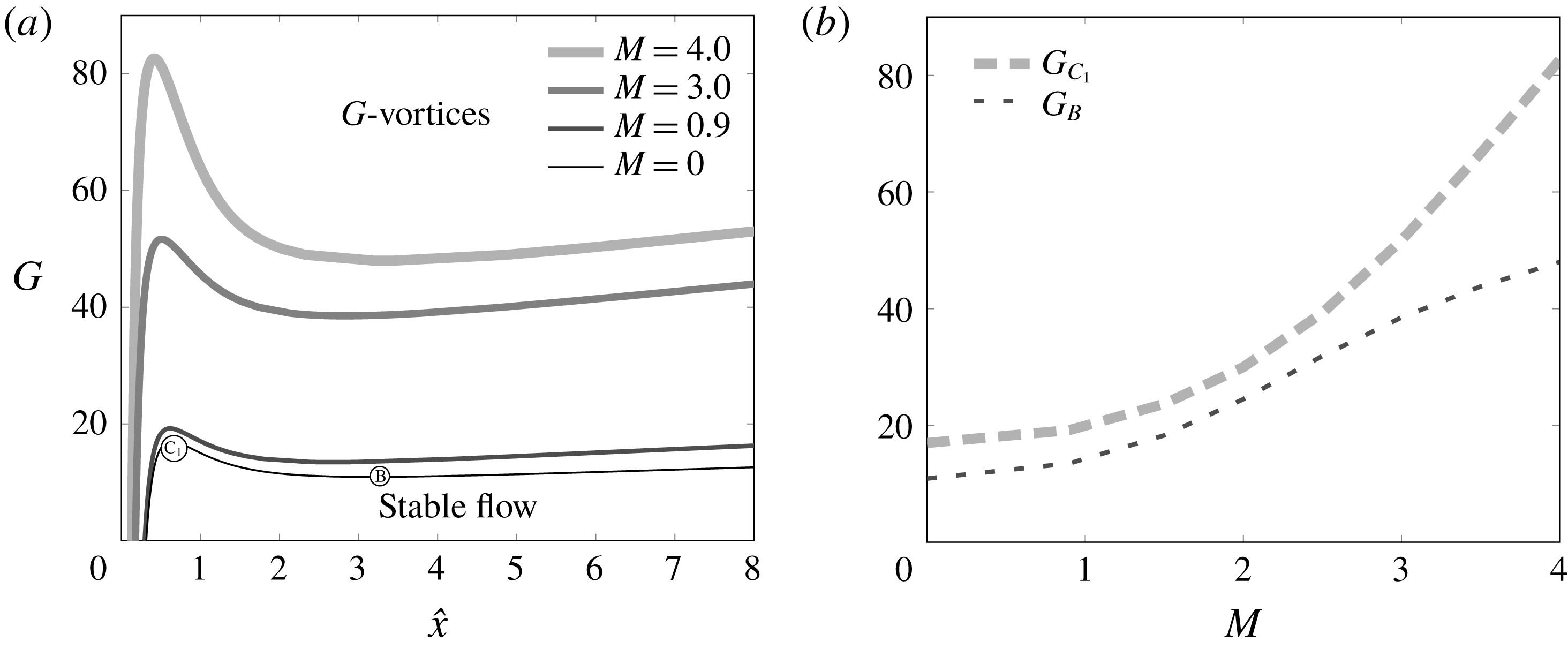
We first study the effect of compressibility on the neutral curves in the steady Görtler case ( ${\mathcal{F}}=0$ ). Figure 2(a) shows the stabilizing influence of the Mach number on the neutral stability curves, i.e. the stable region becomes larger as $M$ increases. This effect is more intense at supersonic Mach numbers in agreement with the results of Viaro & Ricco (Reference Viaro and Ricco2019) and previous studies (El-Hady & Verma Reference El-Hady and Verma1983; Hall & Malik Reference Hall and Malik1989). Figure 2(b) shows that the gap between the Görtler number corresponding to the local maximum, $G_{C_{1}}$ , and the Görtler number corresponding to the local minimum, $G_{B}$ (both represented in figure 2 a), grows as $M$ increases, with $G_{C_{1}}$ influenced the most by compressibility. For $G>G_{C_{1}}$ the perturbation shifts directly from Klebanoff modes to Görtler vortices, whereas for $G<G_{B}$ no Görtler vortices are generated, even though the curvature is present.

Figure 2.

(a) Neutral stability curves, $\hat{x}=\hat{x}_{\unicode[STIX]{x1D70D}_{0}}$ , for different $M$ values, ${\mathcal{F}}=0$ and $k_{y}=2$ . (b) Influence of $M$ on the critical Görtler numbers $G_{B}$ and $G_{C_{1}}$ , shown in (a).

3.2 Effect of frequency on the neutral curves

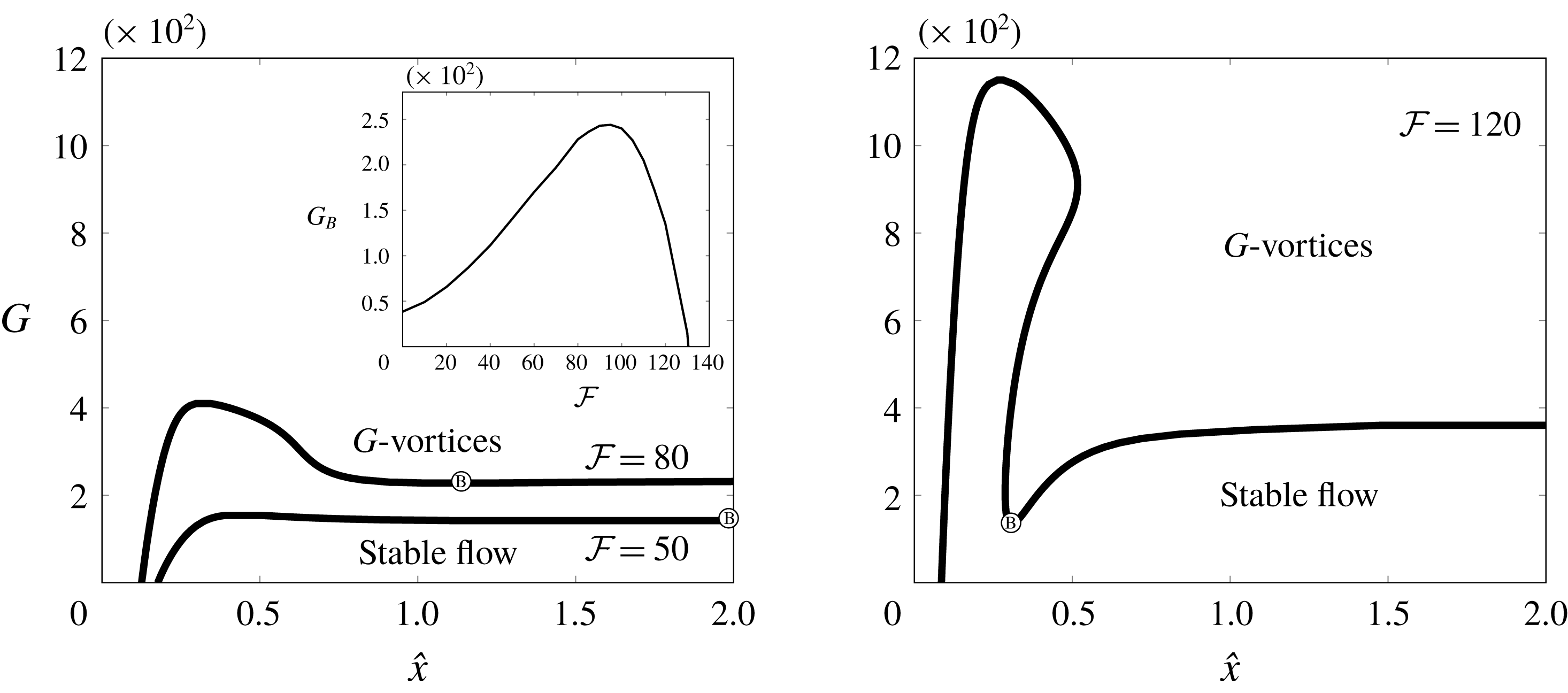
The change of the neutral curve in figure 2(a) as the frequency increases is shown in figures 3 and 4 for $M=3$ . The stable region expands as ${\mathcal{F}}$ grows. The inset of figure 3(a) shows that $G_{B}$ increases with ${\mathcal{F}}$ up to ${\mathcal{F}}=90$ , but it rapidly drops at larger ${\mathcal{F}}$ , as shown in figure 3(b). It reaches zero when ${\mathcal{F}}=130.5$ . For ${\mathcal{F}}<130.5$ , no instability is found in the flat-plate case ( $G=0$ ) other than the $\text{K}$ -modes. For ${\mathcal{F}}>130.5$ two separate stable regions and a new critical $G_{B}$ appear ( $G_{B}=437$ for ${\mathcal{F}}=150$ ). Figure 4 shows that at ${\mathcal{F}}=150$ the stable region $\text{S}_{1}$ is confined by nearly vertical lines, which demonstrates that the effect of curvature on $\text{S}_{1}$ is limited. As ${\mathcal{F}}$ increases, $G_{C_{1}}$ increases rapidly and the vertical lines confining the stable region $\text{S}_{1}$ become more parallel to the ordinate axis.

Figure 3.

Evolution of the neutral stability curves $\hat{x}=\hat{x}_{\unicode[STIX]{x1D70D}_{0}}$ as ${\mathcal{F}}$ increases for $M=3$ and $k_{y}=1$ . Inset: influence of ${\mathcal{F}}$ on $G_{B}$ .

3.3 Regions of instability

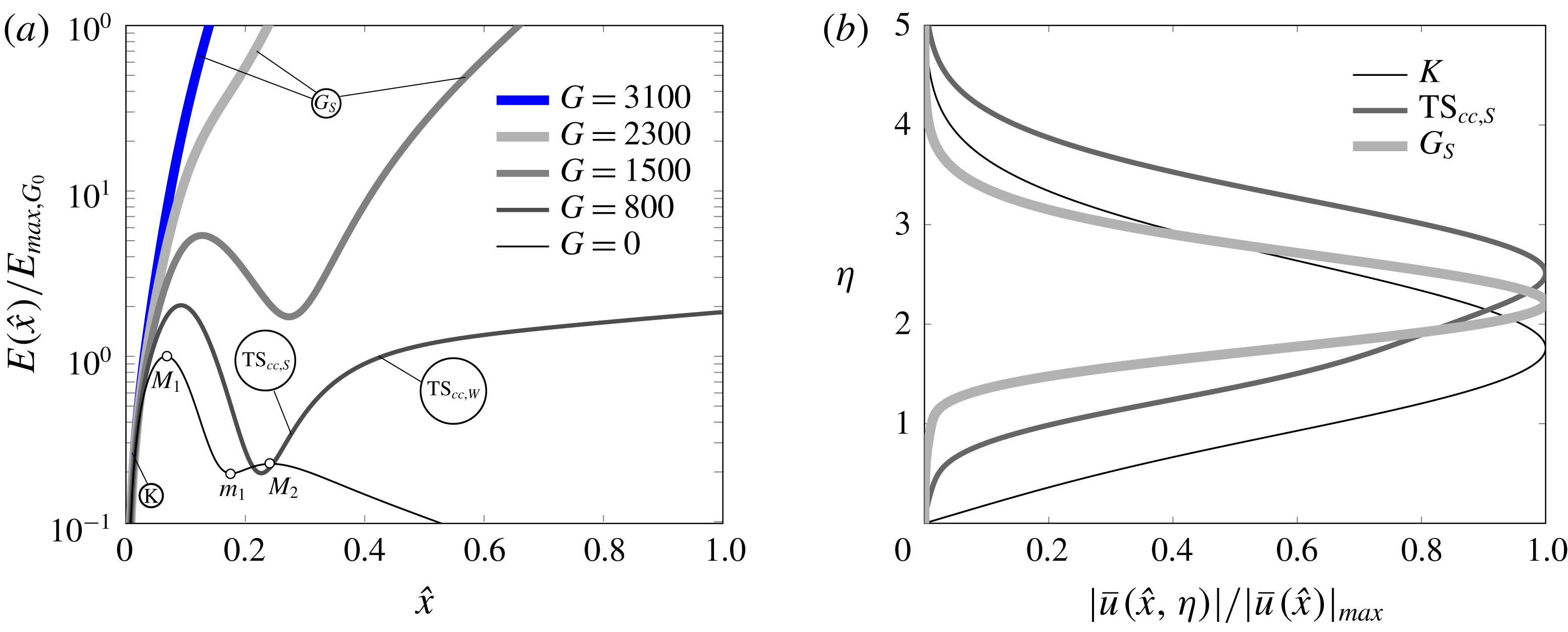
We further analyse the case for ${\mathcal{F}}=150,M=3$ and $k_{y}=1$ , shown in figure 4. At these flow conditions the neutral-stability map reveals that the boundary layer can experience the three types of instability, i.e. the $\text{K}$ -modes, the $\text{TS}_{cc}$ -waves and the $G$ -vortices. We identify the conditions for which these instabilities coexist using figures 5 and 6 to support the discussion. Figure 5(a) shows the $\hat{x}$ evolution of the energy $E(\hat{x})$ , scaled by the maximum value $E_{max,G_{0}}\equiv \max _{\hat{x}}|E(\hat{x})|_{G=0}$ , for five representative Görtler numbers. The energy maxima, $M_{1}$ and $M_{2}$ , and the energy minimum $m_{1}$ identify the conditions for which $\unicode[STIX]{x1D70D}=0$ . 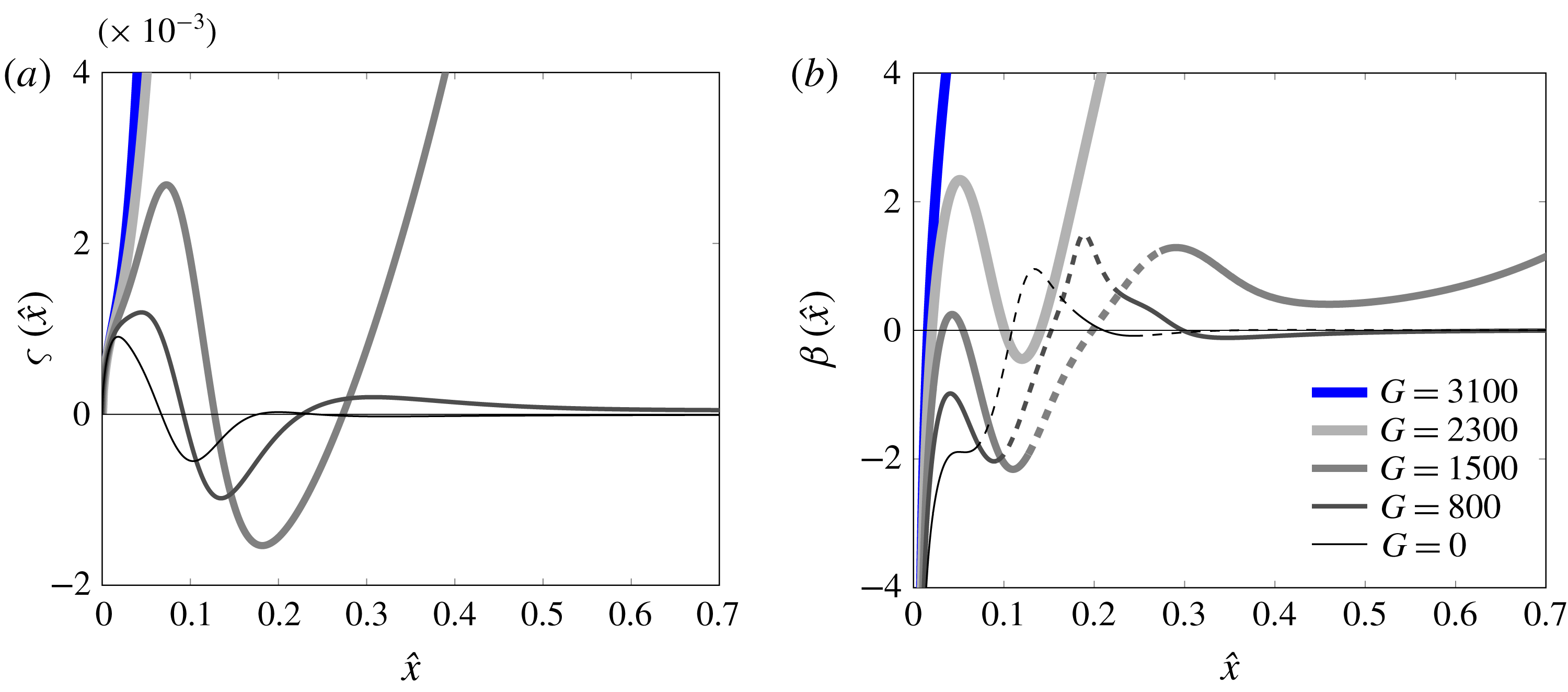Figure 5(b) displays the wall-normal profiles of $|\bar{u}(\hat{x},\unicode[STIX]{x1D702})|/|\bar{u}(\hat{x})|_{max}$ that are representative of the three types of perturbation. Figure 6 shows the $\hat{x}$ evolutions of $\unicode[STIX]{x1D70D}(\hat{x})$ , the growth rate of the perturbation (a), and of $\unicode[STIX]{x1D6FD}(\hat{x})$ , the curvature of the maximum velocity with respect to $\hat{x}$ (b).

Figure 4.

Neutral stability curve, $\hat{x}=\hat{x}_{\unicode[STIX]{x1D70D}_{0}}$ (

), and regions of instability for ${\mathcal{F}}=150$ , $k_{y}=1$ and $M=3$ . The blue full circles, located at $\{0.03,0\}$ , $\{0.3,1000\}$ , $\{1.2,2300\}$ , refer to the velocity profiles shown in figure 5.

Since curvature effects are not at work near the leading edge (Wu et al. Reference Wu, Zhao and Luo2011) and $\hat{x}$ is not large enough for the $\text{TS}$ -wave receptivity mechanism studied by Ricco & Wu (Reference Ricco and Wu2007) to operate, only $\text{K}$ -modes initially grow from the leading edge with $\unicode[STIX]{x1D6FD}<0$ at any $G$ due to the continuous free-stream forcing. The $\text{K}$ -modes either stabilize downstream of the first encountered neutral line at $\hat{x}=\hat{x}_{\unicode[STIX]{x1D70D}_{0}}$ or, for $G>G_{C_{1}}=1792$ , turn directly into $G$ -vortices at $\hat{x}=\hat{x}_{K}$ , indicated by the thick grey dotted line in figure 4 (scenario

$\unicode[STIX]{x1D6FD}$

$\text{S}_{1}$

$G$

$\hat{x}=\hat{x}_{\unicode[STIX]{x1D6FD}_{0}}$

For the flat-plate case ( $G=0$ ), the only growing perturbations are the $\text{K}$ -modes and the $\text{TS}$ -waves. The $\text{K}$ -modes start growing from the leading edge and dissipate rapidly downstream of $M_{1}$ due to viscous effects (Leib et al. Reference Leib, Wundrow and Goldstein1999), as shown in figure 5(a). The combined influence of the frequency and the Mach number triggers the $\text{TS}$ -waves at point $\text{A}_{1}$ , which display a second energy peak at $M_{2}$ . For these flow conditions, the $\text{TS}$ -waves are weaker than the $\text{K}$ -modes and decay downstream of point $\text{A}_{2}$ , shown in figure 4. This case is represented by scenario

$\text{TS}$

As the curvature is introduced, the imbalance between pressure and centrifugal forces energizes both the $\text{K}$ -modes and the $\text{TS}_{cc}$ -waves, but for $G<G_{B}$ this is not sufficient to alter the zero- $G$ pattern qualitatively, thus resulting in a boundary layer without $G$ -vortices. In figure 4 the thin grey dashed line represents the zero- $\unicode[STIX]{x1D6FD}$ streamwise location $\hat{x}=\hat{x}_{TS_{s}}$ where the $\text{TS}_{cc}$ -waves shift from a strong growth ( $\text{TS}_{cc,S}$ , $\unicode[STIX]{x1D6FD}>0$ ) to a weak growth ( $\text{TS}_{cc,W}$ , $\unicode[STIX]{x1D6FD}<0$ ). The key observation here is that the first growth with $\unicode[STIX]{x1D6FD}>0$ downstream of $\text{S}_{1}$ has to be of the $\text{TS}_{cc}$ -wave type because it evolves continuously from the flat-plate scenario for which centrifugal effects are absent. The influence of $G$ on the onset of the $\text{TS}$ -waves is mild as the neutral lines are almost vertical. The negligible influence of the curvature on the $\text{TS}_{cc}$ -waves for $G=O(1)$ is supported by the triple-deck analysis in § 3.4.

For $G>G_{B}$ , the centrifugal effects intensify and the perturbation starts growing again with $\unicode[STIX]{x1D6FD}>0$ further downstream, i.e. the $G$ -vortices appear. At $\hat{x}=\hat{x}_{TS_{w}}$ (thick grey dashed line), the strong-growth Görtler instability ( $G_{S}$ , $\unicode[STIX]{x1D6FD}>0$ ) ensues from the weakly growing $\text{TS}_{cc}$ -waves ( $\text{TS}_{cc\,W}$ , $\unicode[STIX]{x1D6FD}<0$ ). Much further downstream at $\hat{x}=\hat{x}_{G}$ a weak $G$ -vortex growth occurs ( $G_{W}$ , $\unicode[STIX]{x1D6FD}<0$ ) and ultimately a stable boundary layer is computed downstream of $\hat{x}=\hat{x}_{\unicode[STIX]{x1D70D}_{0}}$ (not shown). In the range $G_{C_{2}}<G<G_{D}$ the region of weak $\text{TS}_{cc}$ -wave instability widens downstream. As the curvature increases, the $G$ -vortices move closer to the leading edge and the region of weak $\text{TS}_{cc}$ -waves shortens.

For $G>G_{D}=1350$ , the regime of weak $\text{TS}_{cc}$ -wave growth disappears. The Görtler instability overcomes the weak negative- $\unicode[STIX]{x1D6FD}~\text{TS}_{cc}$ -wave growth and downstream of $\text{S}_{1}$ the perturbations always grow with $\unicode[STIX]{x1D6FD}>0$ . Therefore, for $G>G_{D}$ the pressure–centrifugal imbalance caused by the curvature is sufficiently intense for the perturbation to grow as $G$ -vortices immediately downstream of the stable region. The three types of boundary-layer instability thus occur only in the range $G_{B}<G<G_{D}$ . In the top left corner of figure 4, we observe a very narrow streamwise region for $1400<G<G_{E}=2380$ where the $\text{K}$ -modes show $\unicode[STIX]{x1D6FD}>0$ . Downstream of this thin region, the $\text{K}$ -modes recover the negative curvature and either start decaying in region $\text{S}_{1}$ for $1400<G<G_{C_{1}}$ or turn into $G$ -vortices downstream of $\hat{x}=\hat{x}_{K}$ for $G>G_{C_{1}}.$ For $G>G_{E}$ , the $\text{K}$ -modes show negative $\unicode[STIX]{x1D6FD}$ at any $\hat{x}$ locations upstream of the Görtler growth.

Figure 5.

Evolution of (a) $E(\hat{x})/E_{max,G_{0}}$ and (b) wall-normal profiles of $|\bar{u}(\hat{x},\unicode[STIX]{x1D702})|/|\bar{u}(\hat{x})|_{max}$ for the perturbations corresponding to the blue circles in figure 4 for ${\mathcal{F}}=150$ , $k_{y}=1$ and $M=3$ .

Figure 6.

Evolution of $\unicode[STIX]{x1D70D}(\hat{x})$ (a) and $\unicode[STIX]{x1D6FD}(\hat{x})$ (b), defined in (2.3), for ${\mathcal{F}}=150$ , $k_{y}=1$ and $M=3$ . In (b), the lines are solid when $\unicode[STIX]{x1D70D}>0$ .

3.4 Asymptotic analysis at relatively high frequency

We investigate the effect of curvature for $G=O(1)$ on the highly oblique $\text{TS}$ -waves generated by the receptivity mechanism first studied by Ricco & Wu (Reference Ricco and Wu2007). We are motivated by the numerical result, shown in figure 4, of the negligible influence of curvature on the $\text{TS}$ -wave growth and on the stable region $\text{S}_{1}$ for moderate $G$ values.

The Görtler terms, found in the $y$ -momentum equation (2.11) of Viaro & Ricco (Reference Viaro and Ricco2019) and scaled here in the ( $\bar{x}=k_{x}x$ , $\unicode[STIX]{x1D702}$ ) coordinate system for consistency with the receptivity analysis by Ricco & Wu (Reference Ricco and Wu2007), are

(3.1) $$\begin{eqnarray}\displaystyle {\displaystyle \frac{G}{(2\bar{x})^{1/2}}}\left[2F^{\prime }\bar{u}(\bar{x},\unicode[STIX]{x1D702})-{\displaystyle \frac{{F^{\prime }}^{2}}{T}}\bar{\unicode[STIX]{x1D70F}}(\bar{x},\unicode[STIX]{x1D702})\right]{\displaystyle \frac{\unicode[STIX]{x1D705}}{k_{z}}}, & & \displaystyle\end{eqnarray}$$

where $\unicode[STIX]{x1D705}=k_{z}{\mathcal{F}}^{-1/2}$ and $T(\unicode[STIX]{x1D702})$ is the mean-flow temperature. Ricco & Wu (Reference Ricco and Wu2007) demonstrated that the highly oblique $\text{TS}$ -waves originate from decaying Lam–Rott eigensolutions. Extending Ricco & Wu (Reference Ricco and Wu2007)’s triple-deck analysis to flows over concave surfaces with $\unicode[STIX]{x1D705}\ll 1$ and $G=O(1)$ , in the lower deck (subscript $L$ ) the Görtler terms (3.1) become

(3.2) $$\begin{eqnarray}\displaystyle {\displaystyle \frac{G}{(2\bar{x})^{1/2}}}\left[2F^{\prime \prime }(0)\unicode[STIX]{x1D702}_{L}\bar{u}_{L}-{\displaystyle \frac{{F^{\prime \prime }(0)}^{2}}{T(0)}}\unicode[STIX]{x1D702}_{L}^{2}\bar{\unicode[STIX]{x1D70F}}_{L}\unicode[STIX]{x1D705}\right]{\displaystyle \frac{\unicode[STIX]{x1D705}^{2}}{k_{z}}}\ll {\displaystyle \frac{\unicode[STIX]{x2202}\bar{p}_{L}}{\unicode[STIX]{x2202}\unicode[STIX]{x1D702}_{L}}}=O(1), & & \displaystyle\end{eqnarray}$$

in the main deck (subscript $M$ ) they become

(3.3) $$\begin{eqnarray}\displaystyle {\displaystyle \frac{G}{(2\bar{x})^{1/2}}}\left(2F^{\prime }\bar{u}_{M}-{\displaystyle \frac{{F^{\prime }}^{2}}{T}}\bar{\unicode[STIX]{x1D70F}}_{M}\right){\displaystyle \frac{\unicode[STIX]{x1D705}^{3/2}}{k_{z}}}\ll {\displaystyle \frac{\unicode[STIX]{x2202}\bar{p}_{M}}{\unicode[STIX]{x2202}\unicode[STIX]{x1D702}}}=O(1), & & \displaystyle\end{eqnarray}$$

and in the upper deck (subscript $U$ ) they are

(3.4) $$\begin{eqnarray}\displaystyle {\displaystyle \frac{2G\bar{u}_{U}}{(2\bar{x})^{1/2}}}{\displaystyle \frac{\unicode[STIX]{x1D705}^{2}}{k_{z}}}\ll {\displaystyle \frac{\unicode[STIX]{x2202}\bar{p}_{U}}{\unicode[STIX]{x2202}\unicode[STIX]{x1D702}_{U}}}=O(1), & & \displaystyle\end{eqnarray}$$

where the pressure terms in (3.2), (3.3) and (3.4) are of the same order as the other terms in the triple-deck $y$ -momentum equations of Ricco & Wu (Reference Ricco and Wu2007). The curvature terms are thus negligible at first order and the flat-plate dispersion relation for the streamwise wavenumber $\unicode[STIX]{x1D6FC}_{1}(\bar{x})$ is recovered (Ricco & Wu Reference Ricco and Wu2007),

(3.5) $$\begin{eqnarray}\displaystyle \int _{\unicode[STIX]{x1D702}_{0}}^{\infty }\text{Ai}(\breve{\unicode[STIX]{x1D702}})\text{d}\breve{\unicode[STIX]{x1D702}}-(\text{i}\unicode[STIX]{x1D6FC}_{1})^{-1/3}\left[{\displaystyle \frac{F^{\prime \prime }(0)}{(2x_{1})^{1/2}}}\right]^{5/3}\left[{\displaystyle \frac{\unicode[STIX]{x1D707}(0)}{T(0)^{7}}}\right]^{1/3}\text{Ai}^{\prime }(\unicode[STIX]{x1D702}_{0})=0, & & \displaystyle\end{eqnarray}$$

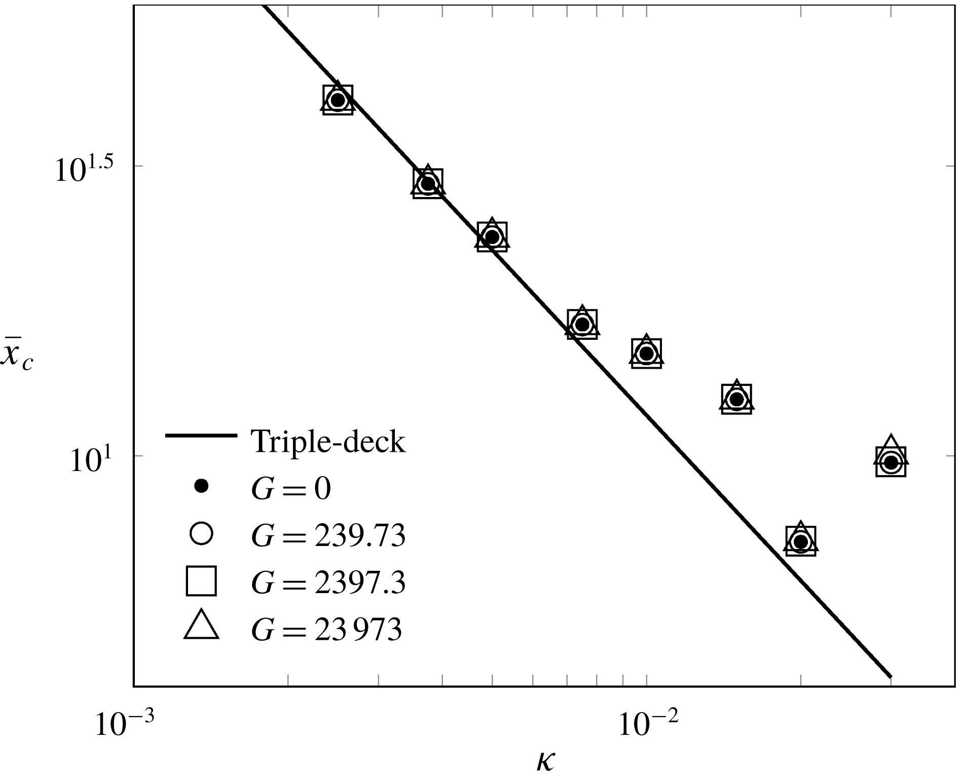
where $\text{Ai}(\unicode[STIX]{x1D702})$ is the Airy function, $x_{1}=\unicode[STIX]{x1D705}\bar{x}=O(1)$ is the scaled streamwise coordinate and $\unicode[STIX]{x1D702}_{0}=-[2\text{i}F^{\prime \prime }(0)\unicode[STIX]{x1D6FC}_{1}x_{1}T(0)/\unicode[STIX]{x1D707}(0)]^{1/3}/[\unicode[STIX]{x1D6FC}_{1}F^{\prime \prime }(0)]$ . Numerical integration of (3.5) gives the local growth rate, $\text{Im}(\unicode[STIX]{x1D6FC}_{1})$ . Figure 7 graphically shows the critical streamwise location $\bar{x}_{c}$ where the $\text{TS}_{cc}$ -waves start to grow as a function of $\unicode[STIX]{x1D705}$ for different $G$ values. Excellent agreement is found between the LUBR computation and the triple-deck theoretical solution, i.e. $\bar{x}_{c}=C\unicode[STIX]{x1D705}^{-1}$ . This comparison allows us to compute the proportionality constant, $C=3.32$ . The effect of the curvature only appears for $\unicode[STIX]{x1D705}\geqslant 0.02$ and $G\geqslant 23\,973$ , which is consistent with the analytical results valid for $\unicode[STIX]{x1D705}\ll 1$ and $G=O(1)$ . These findings give full support to the lines $\hat{x}_{\unicode[STIX]{x1D70D}_{0}}$ confining the stable region $\text{S}_{1}$ being nearly vertical for moderate $G$ values, as shown in figure 4. As the frequency increases, these lines become even more parallel to the ordinate axis and extend to higher $G$ values, which confirms that $\text{TS}$ -waves are not affected by the curvature when the frequency is sufficiently high. This also strengthens the argument that the perturbations downstream of the stable region $\text{S}_{1}$ can be classified as $\text{TS}$ -waves for moderate $G$ .

Figure 7.

Influence of the Görtler number on the streamwise location $\bar{x}_{c}$ as a function $\unicode[STIX]{x1D705}$ for the triple-deck solution (continuous line) and the LUBR solution (symbols) for $M=3$ and $k_{y}=1$ .

Figure 8.

Comparison of the LUBR neutral curve (

) at ${\mathcal{F}}=0$ , $k_{y}=1$ with El-Hady & Verma (Reference El-Hady and Verma1983)’s neutral curves (

) and with Hall (Reference Hall1990)’s neutral curve (

) for $M=0$ (a) and $M=3$ (b). Experimental data by Tani (Reference Tani1962) (●) and Ciolkosz & Spina (Reference Ciolkosz and Spina2006) (▪, ▴), and locations where the $\text{K}$ -modes become $G$ -vortices ( $\hat{x}=\hat{x}_{K}$ , $\cdots \cdots$ ).

3.5 Comparison with experimental data and previous theoretical results

In figure 8, the neutral curves computed by the LUBR equations for ${\mathcal{F}}=0$ and $k_{y}=1$ are compared with neutral curves by other authors (dashed lines) for $M=0$ (a) and for $M=3$ (b). The figure also shows the positions $\hat{x}=\hat{x}_{K}$ where the $\text{K}$ -modes shift to $G$ -vortices (dotted lines) and the streamwise locations and Görtler numbers of experimental data.

For $M=0$ , figure 8(a) shows that the theoretical neutral curve computed by the EV framework of El-Hady & Verma (Reference El-Hady and Verma1983) fails to capture the unstable region near the leading edge where the $\text{K}$ -modes grow downstream. This is expected as the dynamics of $\text{K}$ -modes can only be computed through the inhomogeneous receptivity formalism of Leib et al. (Reference Leib, Wundrow and Goldstein1999) and Wu et al. (Reference Wu, Zhao and Luo2011). The receptivity framework by Hall (Reference Hall1990) includes the effect of the oncoming disturbed flow and is therefore an improvement of Hall (Reference Hall1983)’s approach, where the initial conditions for the parabolic equations modelled vortices that were already inside the boundary layer without accounting for their generation caused by the free-stream disturbances. Hall (Reference Hall1990)’s neutral curve shows good agreement with our $\hat{x}_{K}$ -line, downstream of which the $G$ -vortices evolve from the $\text{K}$ -modes. Nevertheless, Hall (Reference Hall1990)’s curve is unable to predict the $\text{K}$ -mode growth. Tani (Reference Tani1962)’s experimental point of instability at the shortest distance from the leading edge is classified as stable by El-Hady & Verma (Reference El-Hady and Verma1983) and Hall (Reference Hall1990), whereas our computations predict this point as representative of growing $\text{K}$ -modes. All the other points by Tani (Reference Tani1962) fall inside the unstable region and are thus identified as $G$ -vortices. We compare Tani (Reference Tani1962)’s data with the neutral curve for ${\mathcal{F}}=0$ because, although Tani (Reference Tani1962) did not report the dominant frequency of their free-stream disturbance, Wu et al. (Reference Wu, Zhao and Luo2011) showed excellent agreement between these data and their numerical results for steady conditions. The wind-tunnel incompressible data by Boiko et al. (Reference Boiko, Ivanov, Kachanov and Mischenko2010) have been shown by Viaro & Ricco (Reference Viaro and Ricco2018) to fall within the region of Görtler instability.

As in the incompressible case, El-Hady & Verma (Reference El-Hady and Verma1983)’s neutral curve for $M=3$ in figure 8(b) does not predict the algebraic growth from the leading edge, although the agreement with the LUBR solution improves as $\hat{x}$ increases. The experimental data by Ciolkosz & Spina (Reference Ciolkosz and Spina2006) at supersonic conditions, corresponding to perturbations with a spanwise wavelength equal to 0.2 mm, fall in the unstable region and are thus classified as $G$ -vortices. Ciolkosz & Spina (Reference Ciolkosz and Spina2006) also measured the perturbations at the same locations and flow conditions over a flat plate and no growing perturbations were detected. This is also in agreement with our computations as these experimental points all lie in the stable zero- $G$ region downstream of the $\text{K}$ -mode growth.