1. Introduction
The probability density function (p.d.f.) is a fundamental quantity for characterising random values. In turbulence research, particularly in turbulent boundary layers, early studies focused on measuring the p.d.f. of velocity fluctuations in itself and on characterising the statistical properties of the flow field. Klebanoff (Reference Klebanoff1955) measured streamwise velocity fluctuations using a single-wire probe (called an I-probe) at several positions from the wall and calculated the corresponding p.d.f.s. Frenkiel & Klebanoff (Reference Frenkiel and Klebanoff1965) simultaneously measured velocity fluctuations at two points by operating two single-wire probes, separated by a small distance, with constant-temperature anemometry. In these early studies, they observed that streamwise velocity fluctuations showed strong similarity to Gaussian statistics. Therefore, joint p.d.f.s were compared with joint normal distributions in the logarithmic region of the boundary layer (Frenkiel & Klebanoff Reference Frenkiel and Klebanoff1973). Eckelmann (Reference Eckelmann1974) measured the velocity p.d.f. in the viscous sublayer of oil channel flow and found that the p.d.f. of streamwise velocity was symmetric only at
 $y^+ \simeq 13$
, but not Gaussian (the flatness factor was not
 $3$
). At other distances from the wall, the distributions were skewed. Later, a cross-wire probe (called an X-probe) was used to measure both streamwise and vertical (wall-normal) velocity fluctuations. Using this technique, the p.d.f. of instantaneous Reynolds shear stress fluctuations was obtained by Gupta & Kaplan (Reference Gupta and Kaplan1972), Wyngaard & Izumi (Reference Wyngaard and Izumi1973), Lu & Willmarth (Reference Lu and Willmarth1973) and Wallace & Brodkey (Reference Wallace and Brodkey1977).
The issue of spatial resolution of probes (hot-wire and hot-film) was discussed early on, for instance by Johansson & Alfredsson (Reference Johansson and Alfredsson1983), Blackwelder & Haritonidis (Reference Blackwelder and Haritonidis1983) and Ligrani & Bradshaw (Reference Ligrani and Bradshaw1987). Ligrani & Bradshaw (Reference Ligrani and Bradshaw1987) showed that, at a given distance from the wall in the viscous sublayer, the turbulence intensity, flatness factor and skewness factor of longitudinal velocity fluctuations are nearly independent of wire length when the length (
 $\ell$
) is less than
 $20 {-} 25$
times the viscous length scale. The issue of spatial resolution has continued to attract attention, with more recent progress focusing on the development of micro-electro-mechanical systems (MEMS) probes for high-Reynolds-number measurements (Bailey et al. Reference Bailey, Kunkel, Hultmark, Vallikivi, Hill, Meyer, Tsay, Arnold and Smits2010; Samie, Hutchins & Marusic Reference Samie, Hutchins and Marusic2018; Baradel et al. Reference Baradel, Giani, Mery, Combette and Léon2024). Örlü & Alfredsson (Reference Örlü and Alfredsson2010) reported that spatial resolution affects the p.d.f. near the wall (
 $y^+ \lt 150$
) and, consequently, the higher-order moments.
Although the velocity p.d.f. shape is not Gaussian, several approaches have been proposed to approximate its form using fitting parameters. A well-known method is the orthogonal expansion with Gram–Charlier series, which was applied by Frenkiel & Klebanoff (Reference Frenkiel and Klebanoff1973) to streamwise velocity fluctuations. Antonia & Atkinson (Reference Antonia and Atkinson1973) predicted the Reynolds shear stress p.d.f., and the third- and fourth-order moments using the cumulant-discard approach with a joint Gaussian distribution. Similarly, by employing truncated cumulant expressions as an approximation of the p.d.f., Javanović et al. (Reference Javanović, Durst and Johansson1993) derived equations for higher-order moments of turbulent velocity fluctuations. Barndorff-Nielsen (Reference Barndorff-Nielsen1979) introduced a new class of distributions that generalises the Gaussian, the hyperbolic and the so-called exponential power distributions. This idea was applied to characterise the p.d.f. in the boundary layer (Durst, Jovanovic & Kanevce Reference Durst, Jovanovic and Kanevce1987). Ching (Reference Ching1993) and Pope & Ching (Reference Pope and Ching1993) presented exact expressions for the p.d.f. of any quantity measured in a general stationary process, expressed in terms of conditional expectations of both the squared time derivative and the second time derivative of the signal.
Even in homogeneous isotropic turbulence, the p.d.f. of velocity fluctuations need not be Gaussian (Jiménez Reference Jiménez1998). In grid turbulence, where turbulence is still developing, the p.d.f.s indicate sub-Gaussian behaviour, while in the decaying region, they become hyper-Gaussian (Mouri et al. Reference Mouri, Takaoka, Hori and Kawashima2002).
In wall-bounded shear flows, several studies have examined the universality of the p.d.f. shape in channel flows (Dinavahi, Breuer & Sirovich Reference Dinavahi, Breuer and Sirovich1995) and turbulent boundary layers (Tsuji & Nakamura Reference Tsuji and Nakamura1999). When velocity fluctuations are normalised by their mean and standard deviation, it has been reported that p.d.f. shapes become universal in certain regions away from the wall. These results were first obtained at low Reynolds numbers, but the same idea was later verified at relatively high Reynolds numbers by Lindgren, Johansson & Tsuji (Reference Lindgren, Johansson and Tsuji2004) and Zhou & Klewicki (Reference Zhou and Klewicki2015). Lindgren et al. (Reference Lindgren, Johansson and Tsuji2004) reported that the self-similar p.d.f. region extends beyond the universal overlap region, starting at
 $y^+ \simeq 160$
and reaching out to
 $y/\delta _{95} \simeq 0.3$
. Zhou & Klewicki (Reference Zhou and Klewicki2015) found that the self-similar region is estimated to lie within the bounds
 $2.6\sqrt {\delta ^+}$
and
 $0.3\delta ^+$
, which are inside the bounds of the self-similar inertial domain associated with the mean momentum equation. Here, the boundary layer thicknesses
 $\delta _{95}$
and
 $\delta$
are defined as the positions at which the local mean velocity reaches
 $95\,\%$
and
 $99\,\%$
of free stream velocity, respectively. Ge, Yang & Marusic (Reference Ge, Yang and Marusic2019) proposed an alternative scale for normalising velocity fluctuations, instead of the standard deviation. This scale is a direct consequence of Townsend’s attached-eddy hypothesis. By analysing direct numerical simulation (DNS) data at
 $R_\tau =1000$
and experimental data at
 $R_\tau \simeq 10\,000$
, they showed that the velocity p.d.f. tails collapse in the region
 $3\sqrt {\delta ^+} \le y^+ \le 0.2\delta ^+$
.
From the previous brief review of p.d.f. studies in turbulent boundary layers, it is still not clearly understood how the p.d.f.s vary at higher Reynolds numbers (
 $10\,000 \le R_\tau$
), whether universal shapes appear and where they are realised. In this paper, we investigate the p.d.f. of streamwise velocity fluctuations in a zero-pressure-gradient turbulent boundary layer, while taking into account the spatial resolution of the hot-wire probe. By analysing p.d.f. shapes across the boundary layer, we identify the invariant p.d.f. region, where the shape does not change, and clarify where it becomes universal, independent of Reynolds number. Finally, we discuss the relation between the invariant p.d.f. region and the log-law region of the mean velocity and turbulence intensity.
The paper is organised as follows. The experimental conditions are described in § 2 and § 3 provides details of the data processing. The discussions and conclusions are presented in §§ 4 and 5, respectively.
2. Experimental method
2.1. Wind tunnel
Velocity fluctuations in high-Reynolds-number, zero-pressure-gradient turbulent boundary layers were measured using a single hot-wire probe in the low-noise wind tunnel at the Railway Technical Research Institute (RTRI) in Maibara, Japan. The wind tunnel was constructed to support research and development on aerodynamic noise, and other issues related to the Shinkansen and other high-speed railways (see figure 1). The closed test section, 5 m wide
 $\times$
 $3$
m high
 $\times$
 $20$
m long, consists of an upstream wind tunnel section (
 $6.5$
m long) and a downstream section (
 $13.5$
m long), both of which are movable. It has been used to test and improve aerodynamic forces and drag characteristics of train models, and to study the surrounding flow field. A flat plate was placed inside the test section, and the streamwise velocity fluctuations were measured using constant-temperature anemometry with an I-type probe at positions
 $6.0$
,
 $14.4$
and
 $18.7$
m from the leading edge.
Plane view of wind tunnel facility at RTRI wind tunnel technical center (https://www.rtri.or.jp/rd/maibara-wt/). The unit of length is mm.

Figure 1. Long description
The diagram presents a plane view of a wind tunnel facility at the RTRI Wind Tunnel Technical Center. The facility includes a heat exchanger, silencers, a honeycomb structure, corner vanes, a steel screen, a fan, and a test section within an anechoic room. The dimensions of the components are labeled in millimeters, with the overall length of the facility being 84000 millimeters and the height 30000 millimeters. The test section measures 20000 by 20000 millimeters, and the anechoic room extends 22000 millimeters. The wind direction is indicated by an arrow, and there is an exhaust port for smoke tests labeled as a breather.
2.2. Velocity measurement
Velocity fluctuations were measured using an I-type probe. A tungsten wire with a diameter of
 $\phi = 2.5\,\unicode{x03BC}$
m was copper-plated (the stub part) and soldered onto sharp prongs made of stainless steel. The diameter and length of the stub were
 $\phi _s = 20\,\unicode{x03BC}$
m and
 $\ell _s = 0.45$
mm, respectively. The sensitive length of the wire was
 $\ell \simeq 0.4$
mm. The hot wire was operated with an in-house constant-temperature anemometer at an overheat ratio of
 $1.5$
. The prong was bent to minimise flow disturbance near the wall (pitch angle
 $\theta = 5^\circ$
). The data were sampled using a 16-bit A/D converter at 60 kHz, with a total sampling time
 $T$
sufficient to ensure convergence of the p.d.f., i.e.
 $10^4 \lt TU_0/\delta$
, corresponding to
 $5.4 \times 10^6$
data points at each location. The cutoff frequency of the low-pass filter was determined using a square-wave test, which was approximately half of the sampling frequency and checked by the decay of energy spectrum in the dissipation range. The hot wire was statically calibrated in situ against a pitot-static tube ① in the free stream before and after each boundary-layer traverse. The pitot-static tube was connected to a calibration-certified FCO510 (Furness).
The other pitot-static tube ② was placed 0.4 m above the side wall (outside the boundary layer) and
 $12$
m downstream from the leading edge. As the readings from pitot tubes ① and ② agreed within an accuracy of
 $1$
%, the flow inside the wind tunnel was considered uniform. Wall static pressure holes were arranged at
 $10$
positions along the side wall in the streamwise direction. Using the wall pressure
 $P_w(x)$
at streamwise location
 $x$
, the pressure coefficient was defined as
 $C_p= [ P_w(x)-P_w(x_r) ]/(\rho U_0^2/2)$
, where
 $x_r =14.4$
. The value of
 $C_p$
was less than 0.02 and nearly zero for
 $x \gt x_r$
.
The importance of wire length was notably emphasised by Johansson & Alfredsson (Reference Johansson and Alfredsson1983), who was among the first to demonstrate the effects of imperfect spatial resolution on hot-wire anemometry measurements in turbulent boundary layers. In addition to the issue of spatial resolution, Joule heat conduction to the wire supports and the frequency response must also be considered for accurate measurements near the wall, particularly when evaluating the peak of turbulence intensity at
 $y^+ \simeq 15$
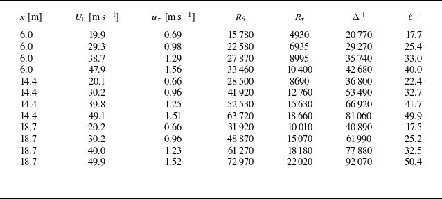
. Several methods have been proposed to correct these artificial effects and to evaluate the peak intensity more reliably. These methods are well summarised by Miller, Estejab & Bailey (Reference Miller, Estejab and Bailey2014) and recent progress with MEMS probes has been reported by Baradel et al. (Reference Baradel, Giani, Mery, Combette and Léon2024). The accuracy of hot-wire measurement relates to several factors, such as space-resolution, end condition (Miller et al. Reference Miller, Estejab and Bailey2014), heat conduction effect (Samie et al. Reference Samie, Hutchins and Marusic2018), sampling frequency, probe intrusivity (Baradel et al. Reference Baradel, Giani, Mery, Combette and Léon2024) and so on. Considering these previous studies and their remarks, we carefully made a hot-wire probe, set it near the wall and performed the data sampling. In the present study, the measured data (as shown table 1) were analysed without any correction.
Statistical properties of the boundary layers.
 $U_0$
is the free stream velocity and
 $u_\tau$
is the friction velocity.
 $R_\theta$
is the Reynolds number based on the momentum thickness
 $\theta$
and the free stream velocity,
 $R_\theta = U_0 \theta / \nu$
, where
 $\nu$
is the kinematic viscosity.
 $R_\tau$
is the Reynolds number based on the boundary-layer thickness
 $\delta$
and the friction velocity,
 $R_\tau = u_\tau \delta / \nu$
, where
 $\delta$
is defined as the position at which the local mean velocity reaches
 $0.99 U_0$
.
 $\Delta ^+$
and
 $\ell ^+$
denote the Rotta–Clauser boundary-layer thickness and the hot-wire sensitive length, respectively, normalised by inner variables.

Table 1. Long description
The table presents statistical properties of boundary layers, comparing various parameters across different measurements. It includes columns for distance in meters, free stream velocity in meters per second, friction velocity in meters per second, Reynolds number based on momentum thickness, Reynolds number based on boundary-layer thickness, Rotta-Clauser boundary-layer thickness normalized by inner variables, and hot-wire sensitive length normalized by inner variables. The table has 10 rows and 8 columns, providing detailed data for each parameter. Notable trends include increasing Reynolds numbers and friction velocities with higher free stream velocities.
2.3. Wall shear stress measurement
The friction velocity was measured using oil-film interferometry (Naughton & Sheplak Reference Naughton and Sheplak2002). This methodology is well established and has been applied to wall shear stress measurements in turbulent boundary layers (see, for example, Österlund Reference Österlund1999). In the present set-up, a small CMOS camera was positioned beneath the flat plate to record the fringe patterns. Details of the arrangement are provided in Appendix A. The skin-friction coefficient, defined as
 $c_{\!f} \equiv 2(u_\tau /U_0)^2$
, was found to be well represented by the relation
 \begin{equation} \frac {c_{\!f}}{2} = \left [ \frac {1}{\kappa } \ln \left ( \frac {u_\tau \Delta }{\nu } \right ) + C \right ]^{-2}, \end{equation}
where
 $\varDelta$
is the Rotta–Clauser boundary-layer thickness, as introduced by Fernholz & Finley (Reference Fernholz and Finley1996). Based on a survey of previous measurements, typical values are
 $\kappa = 0.40$
and
 $C = 4.3$
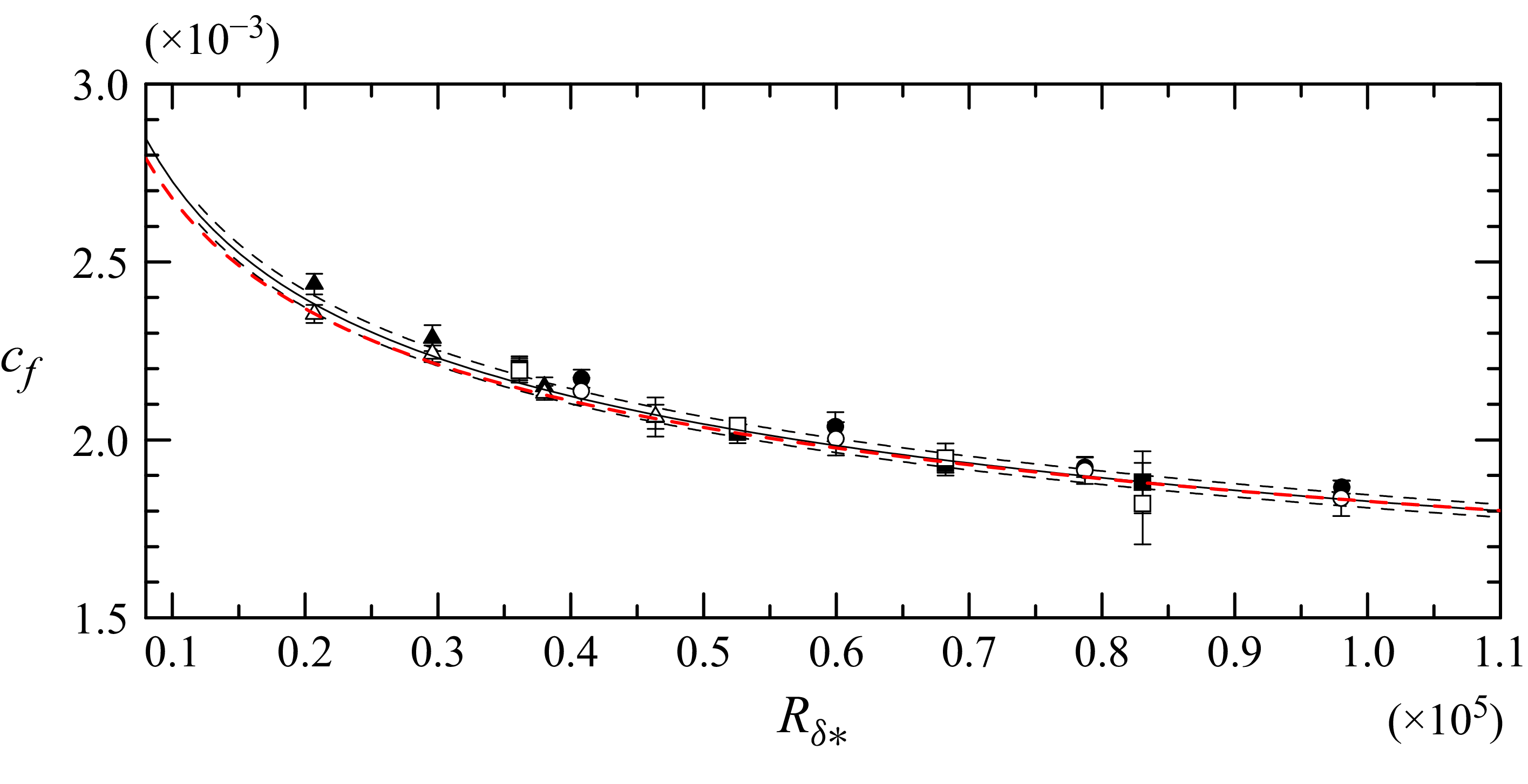
. The present results are summarised in figure 3, and least-squares fitting of (2.1) yielded
 $\kappa = 0.384$
and
 $C = 3.1$
.
I-probe arrangement on the plate. It can be traversed up to
 $400$
mm from the wall. A small thermistor was mounted on the wall to monitor the temperature during the measurements. A small transparent plate was used for the OFI measurement, as shown in figure 9.

Figure 2. Long description
A close-up view of an I-probe arrangement on a transparent plate. The probe is mounted on a circular base and extends vertically. The plate has several small holes around the probe. A small thermistor is mounted on the wall to monitor the temperature during measurements. The setup is used for optical flow imaging (OFI) measurements.
Skin-friction coefficient measured by oil-film interferometry (OFI).
 $\triangle$
,
 $x = 6.0$
m (
 $\lambda$
-method);
 $\square$
,
 $x = 14.4$
m (
 $\lambda$
-method);
 $\circ$
,
 $x = 18.7$
m (
 $\lambda$
-method);
 $\blacktriangle$
,
 $x = 6.0$
m (
 $XT$
-method);
 $\blacksquare$
,
 $x = 14.4$
m (
 $XT$
-method);
 $\bullet$
,
 $x = 18.7$
m (
 $XT$
-method). The solid line represents (2.1) with
 $\kappa = 0.384$
and
 $C = 3.1$
. The dashed lines indicate a
 $\pm 1\,\%$
variation. The red dash-dotted line corresponds to (2.1) with
 $\kappa = 0.40$
and
 $C = 4.3$
(Fernholz & Finley Reference Fernholz and Finley1996).
 $R_{\delta *}$
is defined as
 $u_\tau \Delta /\nu$
.

Figure 3. Long description
The line graph displays the skin-friction coefficient measured by oil-film interferometry. The x-axis represents the variable R delta star, ranging from 0.1 to 1.1 times 10 to the power of 5. The y-axis represents the skin-friction coefficient, ranging from 1.5 to 3.0 times 10 to the power of -3. Multiple data series are plotted, including solid lines, dashed lines, and a red dash-dotted line, each representing different methods and variations. Data points with error bars are scattered across the graph, indicating measured values and their uncertainties. All values are approximated.
3. Probability density function analysis
The p.d.f. of the streamwise velocity component was carefully analysed and one measure used to characterise the p.d.f. is introduced here: the Kullback–Leibler divergence (KLD, also known as relative entropy). This measure, originally introduced by Kullback (Reference Kullback1959) and later adopted as a fundamental quantity in information theory (Amari Reference Amari1985), is defined as
 \begin{equation} D(P \parallel Q) = \sum _{s_i \in \mathbf{s}} P(s_i) \ln \left [ \frac {P(s_i)}{Q(s_i)} \right ], \end{equation}
where
 $P(s)$
and
 $Q(s)$
are discrete probability distributions defined on the set
 ${\mathbf s} = \{s_1, s_2, s_3, \ldots , s_n\}$
. The KLD is always non-negative and becomes zero only when
 $P(s)$
is identical to
 $Q(s)$
. The closer
 $P(s)$
and
 $Q(s)$
are to one another, the smaller the value of KLD. Thus, the KLD provides a quantitative measure of the similarity between two distributions. In the present analysis,
 $Q(s)$
was taken to be a Gaussian profile, and
 $P(s)$
was set as the measured p.d.f. of the velocity at a distance
 $y$
from the wall. The instantaneous streamwise velocity was decomposed into mean and fluctuation as
 $\tilde {u} = U + u^{\prime}$
. The normalised velocity was defined as
 $u \equiv u^\prime/u_r$
, where
 $u_r$
is the standard deviation of
 $u^\prime$
. Instead of using the friction velocity,
 $u_r$
was regarded as the characteristic velocity scale and the analysis was conducted in terms of the normalized velocity
 $u$
.
It should be noted that the KLD depends on the discretisation of the state variable, i.e. the bin size of
 $\mathbf{s}$
. In the present analysis, the bin size used to compute the p.d.f.s was fixed at
 $0.2u_r$
for all datasets, following the procedure described by Tsuji & Nakamura (Reference Tsuji and Nakamura1999) and Tsuji, Lindgren & Johansson (Reference Tsuji, Lindgren and Johansson2005). When the bin size is varied, the resulting KLD value also changes. Skewness (third-order moment) and flatness (fourth-order moment) are sometimes employed to characterise p.d.f. shapes. However, they capture only limited aspects of the distribution, as can be understood from the Gram–Charlier expansion, an orthogonal expansion whose coefficients are related to the moments of the p.d.f. In contrast, the KLD is a mathematically well-defined measure of distance in probability space and provides a more comprehensive characterisation of distributional differences.
4. Results and discussions
4.1. Invariant p.d.f. regions
Figure 4 shows the mean velocity, KLD and turbulence intensity distributions at different Reynolds numbers. The mean velocity profile follows the log-law relation, plotted as a solid line,
 $U^+=1/\kappa \ln (y^+)+B$
, where
 $\kappa = 0.384$
and
 $B = 4.17$
are the values suggested by Nagib & Chauhan (Reference Nagib and Chauhan2008) and Chauhan, Monkewitz & Nagib (Reference Chauhan, Monkewitz and Nagib2009). The solid lines agree well with the present measurements. However, because the velocity was measured at discrete points, it is difficult to evaluate the local slope
 $y^+ \textrm {d}U^+/\textrm {d}y^+$
and thereby determine the log-law region with high accuracy. The KLD varies with distance from the wall. It reaches a minimum at
 $y^+ \simeq 50$
, indicating that at this location, the probability density of
 $u$
most closely resembles a Gaussian distribution among the measured p.d.f.s. This position is denoted as
 $y^+_p$
.
Mean velocity, KLD and turbulence intensity profiles. Panels (a), (d) and (g) show profiles for
 $\textit{Re}_\tau = 2130$
at KTH measured by
 $d=2.5$
 $\unicode{x03BC}$
m and
 $\ell ^+$
= 13.1; panels (b), (e) and (h) correspond to
 $\textit{Re}_\tau = 6935$
at RTRI; panels (c), (f) and (i) correspond to
 $\textit{Re}_\tau = 15\,070$
at RTRI. The solid line in the mean velocity plot represents
 $U^+ = (1/\kappa )\ln (y^+) + B$
, with
 $\kappa = 0.384$
and
 $B = 4.17$
. Solid circles in panels (d), (e) and (f) are invariant p.d.f. regions. The red dashed line denotes the KLD of invariant p.d.f. region I and the blue dashed line denotes the KLD of invariant p.d.f. region II. The dashed lines in panels (g), (h) and (i) represent fitting curves given by (4.1).

Figure 4. Long description
The line graph consists of nine panels arranged in a 3x3 grid. Panels (a), (d), and (g) display profiles measured at KTH using a specific method with a defined parameter. Panels (b), (e), and (h) correspond to measurements at RTRI. Panels (c), (f), and (i) also correspond to measurements at RTRI. The x-axis represents the dimensionless wall-normal coordinate, while the y-axis varies: mean velocity in panels (a), (b), and (c); KLD in panels (d), (e), and (f); and turbulence intensity in panels (g), (h), and (i). The solid line in the mean velocity plots represents a logarithmic profile. Solid circles in panels (d), (e), and (f) indicate invariant probability density function (p.d.f.) regions. The red dashed line denotes the KLD of invariant p.d.f. region I, and the blue dashed line denotes the KLD of invariant p.d.f. region II. The dashed lines in panels (g), (h), and (i) represent fitting curves given by a specific equation. All values are approximated.
Where the KLD remains constant, the p.d.f. shapes do not change; this corresponds to the invariant p.d.f. region. For the low-Reynolds-number case (
 $\textit{Re}_\tau = 2130$
), only one invariant p.d.f. region was observed. This situation has been reported previously in the range
 $1300 \le R_\theta \le 13\,000$
(
 $435 \le \textit{Re}_\tau \le 4080$
) by Tsuji & Nakamura (Reference Tsuji and Nakamura1999) and Tsuji et al. (Reference Tsuji, Lindgren and Johansson2005). The invariant region is located close to the mean-velocity log region and was evaluated as
 $150 \le y^+ \le y_e^+$
, where the end position
 $y_e^+$
was empirically determined as
 $y_e^+ \simeq 0.049 \Delta ^+$
, with
 $\varDelta$
denoting the Rotta–Clauser boundary-layer thickness. At higher Reynolds numbers, this single invariant region splits and a second invariant region appears. These are hereafter referred to as invariant p.d.f. region I and region II. Region I is located within
 $100 \lesssim y^+ \lesssim 200$
, while region II extends over
 $y^+_{II,{str}} \lesssim y^+ \lesssim y^+_{II,{end}}$
. The detailed discussion of
 $y^+_{II,{str}}$
and
 $y^+_{II,{end}}$
will be given in § 4.3. The KLD values in regions I and II, plotted by the red and blue dashed lines, respectively, appear to be independent of Reynolds number. However, the KLD in region II is larger than in region I. The intermediate region between regions I and II is referred to as the transition region for convenience. It should be noted that the appearance of two invariant regions is a feature of relatively high Reynolds numbers (
 $\textit{Re}_\tau \simeq O(10^4)$
).
By calculating the slope of the mean velocity using log-law fitting over the invariant regions, values of
 $\kappa \simeq 0.41$
and
 $\kappa \simeq 0.38$
were obtained for regions I and II, respectively. In region I, a small hump appears at
 $y^+ \simeq 50$
(this corresponds to the minimum-KLD location
 $y_p^+$
discussed by Tsuji et al. Reference Tsuji, Lindgren and Johansson2005). This hump reduces the local slope of the mean velocity profile or, equivalently, increases the fitted value of
 $\kappa$
. In the transition region,
 $200 \lesssim y^+ \lesssim y^+_{II,{str}}$
, the KLD gradually increases. A similar trend is observed in the variation of skewness, with the zero crossing of skewness located within the transition region. The slope of the log-law fit scatters within the range
 $0.38 \lesssim \kappa \lesssim 0.41$
, depending on the Reynolds number and the width of the transition region. Within invariant region I, the turbulent-intensity profile exhibits a plateau-like shape, but it decreases towards the outer invariant region II. These trends suggest that the attached-eddy (AE) model may be applicable in region II. Further discussion is provided in § 4.3. The p.d.f.s in the invariant regions are shown in figure 5. In region I, the p.d.f.s are nearly symmetric in both the core and tail parts. In contrast, in region II, they show an asymmetry in core part. And the negative tails are close to Gaussian, whereas the positive tails are suppressed. At high Reynolds numbers, these features are consistently observed. For low Reynolds numbers, where only one invariant p.d.f. region exists, the characteristics of the p.d.f.s were discussed in detail by Tsuji et al. (Reference Tsuji, Lindgren and Johansson2005). Ge et al. (Reference Ge, Yang and Marusic2019) reported the absence of a self-similar p.d.f. profile in the region
 $3\sqrt {\textit{Re}_\tau } \le y^+ \le 0.2 \delta ^+$
for Reynolds numbers in the range
 $2700 \le \textit{Re}_\tau \le 13\,000$
. This may be because the p.d.f.s from region I to region II were implicitly compared. The invariant p.d.f. regions I and II are located at different wall-normal positions, and region II emerges only at higher Reynolds numbers. Self-similar p.d.f.s exist in region I across both low and high Reynolds numbers, whereas an additional set of self-similar p.d.f.s arises in region II only when
 $\textit{Re}_\tau \simeq O(10^4)$
.
(a) P.d.f.s in invariant region I. (b) P.d.f.s in invariant region II.
 $\triangle$
, profile for
 $\textit{Re}_\tau = 6935$
;
 $\times$
, profile for
 $\textit{Re}_\tau = 15\,070$
.

Figure 5. Long description
Two line graphs compare probability density functions (p.d.f.s) in invariant regions I and II. The x-axis represents the variable u, ranging from -4.0 to 4.0, while the y-axis represents the probability density function p(u), ranging from 10^-5 to 10^-1. Each graph contains multiple data points represented by different symbols, such as crosses and squares, and a red line indicating a reference distribution. The insets in both graphs provide a zoomed-in view of the p.d.f.s around the central region of u, highlighting the detailed behavior of the distributions. The data points in both graphs show a symmetric distribution around u equals 0, with the probability density decreasing as the absolute value of u increases. The red line serves as a comparison to the observed data, illustrating deviations from the reference distribution. All values are approximated.
We have found the two invariant p.d.f. regions in high-Re turbulent boundary layers. In the next subsections, the turbulent intensity profiles are studied in detail from the point of PDF invariance.
4.2. Plateau region of the turbulent-intensity profile
In this section, the feature of invariant p.d.f. region I and its relation to the turbulent intensity profile is studied. From these discussions, the empirical relation to predict the maximum turbulent intensity is reported.
The turbulent-intensity distribution attains its maximum value,
 $u^+_{r,max }$
, around
 $y^+ \simeq 15$
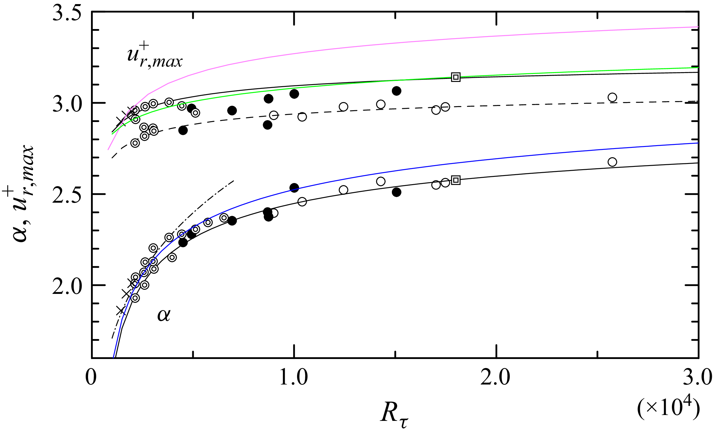
, as previously reported by Fernholz et al. (Reference Fernholz, Krause, Nockemann and Schober1995). This value is plotted in figure 6 as a function of Reynolds number. Only the present data obtained under the condition
 $\ell ^+ \lt 26$
are shown, and they are approximately
 $5\,\%$
smaller than the empirical relations reported by Samie et al. (Reference Samie, Hutchins and Marusic2018) and Chen & Sreenivasan (Reference Chen and Sreenivasan2022). The solid black line represents the formula derived from the finite-dissipation assumption, while the green line corresponds to the attached-eddy model. Both exhibit similar trends, making it difficult to distinguish between them even at the present Reynolds numbers. Although the present experimental values are smaller than the empirical relations, this discrepancy is attributed to the spatial-resolution limitation of the hot-wire probe. Beyond the peak position (
 $y^+ \simeq 15$
) and towards the log region, the turbulent-intensity distributions can be empirically approximated by the relation
 \begin{equation} u_{r,\textit{expand}}^+ = \alpha + \beta _1 \big(y^+ - \gamma \big)^{-1} + \beta _2 \big(y^+ - \gamma \big)^{-2} + {\cdots} , \end{equation}
where
 $\alpha$
is the asymptotic value, i.e.
 $\lim _{y^+ \to \infty } u_{r,\textit{expand}}^+$
, and
 $\gamma$
is a small positive constant, typically
 $\gamma \simeq 5$
(Tsuji & Nakamura Reference Tsuji and Nakamura1999; Tsuji et al. Reference Tsuji, Lindgren and Johansson2005). The coefficients
 $\beta _i$
(
 $i=1,2,{\cdots}$
) depend on the Reynolds number. The dashed lines in figure 4(g, h, i) represent the fitted relations obtained from (4.1). This relation was previously confirmed in the range
 $30 \le y^+ \le y_r^+$
, where
 $y_r^+ \simeq 0.021\Delta ^+ + 96.5$
for
 $R_\theta \lt 13\,000$
(Tsuji et al. Reference Tsuji, Lindgren and Johansson2005). In the present higher Reynolds number cases, (4.1) is also valid in invariant region I and in the transient region, but not in region II. The Reynolds-number dependence of
 $\alpha$
is plotted in figure 6 and is empirically fitted by the relation
 \begin{equation} \alpha = \left [ 10.73 - 47.35\,\textit{Re}_\tau ^{-1/4} \right ]^{1/2}. \end{equation}
Maximum value of the streamwise velocity root mean square (r.m.s.) plotted against Reynolds number. Solid circles (
 $\bullet$
) denote data measured with spatial resolution
 $\ell ^+ \leqslant 26.0$
, while open circles (
 $\circ$
) correspond to
 $\ell ^+ \gt 26.0$
.
 $\circledcirc$
, KTH data measured at
 $x = 5.5$
m from the leading edge with
 $\ell ^+ \leqslant 25.0$
;
 $\boxdot$
, data from Samie et al. (Reference Samie, Hutchins and Marusic2018) at
 $R_\tau = 18\,000$
;
 $\times$
, DNS data of a boundary layer from Sillero, Jimenéz & Moser (Reference Sillero, Jimenéz and Moser2013). The solid line represents the empirical relation
 $u^{+}_{r,max } = [11.5 - 19.3 R_\tau ^{-1/4} ]^{1/2}$
from Chen & Sreenivasan (Reference Chen and Sreenivasan2022) and the dashed line shows its 95 % confidence bound. The solid green line represents
 $u^{+}_{r,max } = [3.54 + 0.646 \ln (R_\tau ) ]^{1/2}$
from Samie et al. (Reference Samie, Hutchins and Marusic2018). The lower plots show the Reynolds-number dependence of
 $\alpha$
, with the same symbols as those for the
 $u^{+}_{r,max }$
distribution. The solid black line represents
 $\alpha = [10.73 - 47.35 R_\tau ^{-1/4}]^{1/2}$
, the solid blue line represents
 $\alpha = [22 - 470/U_0^+ ]^{1/2}$
from Monkewitz & Nagib (Reference Monkewitz and Nagib2015), and the dash-dotted line shows the empirical relation
 $\alpha = 0.33 \textit{Re}_\theta ^{0.21}$
obtained at low Reynolds numbers (Tsuji & Nakamura Reference Tsuji and Nakamura1999).

Figure 6. Long description
The line graph displays the maximum value of the streamwise velocity root mean square plotted against Reynolds number. Solid circles represent data measured with spatial resolution, while open circles correspond to different spatial resolution. Various datasets are included: KTH data measured at a specific distance from the leading edge, data from Samie et al. (2018), and DNS data from Sillero, Jimenz & Moser (2013). The solid line represents an empirical relation from Chen & Sreenivasan (2022), and the dashed line shows its 95% confidence bound. The solid green line represents data from Samie et al. (2018). The lower plots show the Reynolds-number dependence of alpha, with the same symbols as those for the distribution. The solid black line represents an empirical relation, the solid blue line represents data from Monkewitz & Nagib (2015), and the dash-dotted line shows an empirical relation obtained at low Reynolds numbers (Tsuji & Nakamura 1999). All values are approximated.
We assume that
 $\alpha$
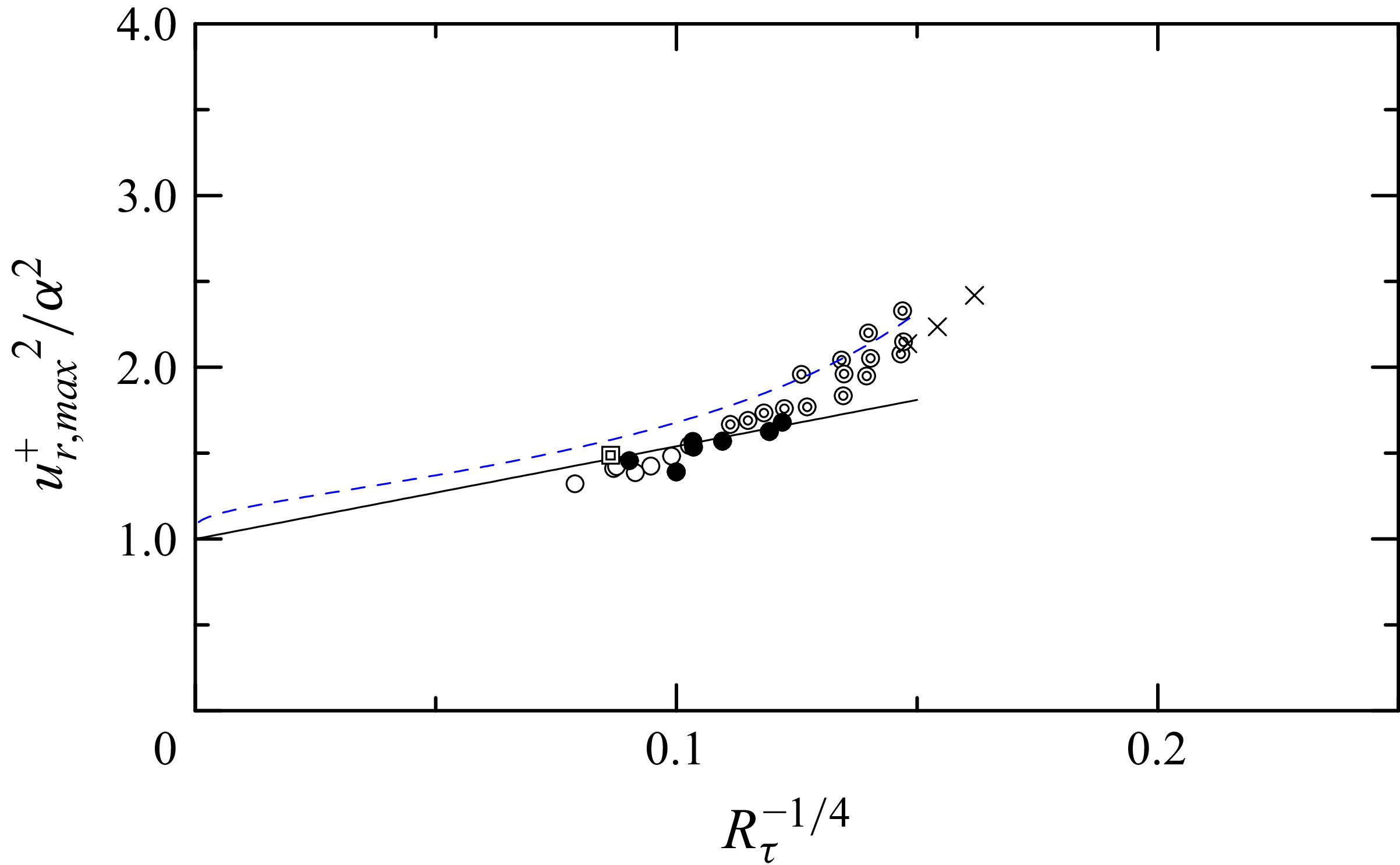
is not affected by the spatial resolution of the hot wire; therefore, all the data in table 1 are plotted in figure 6. Predicting the peak turbulent intensity
 $u^{+}_{r,max }$
at high Reynolds numbers has long been an important topic and several correction methods for hot-wire resolution have been proposed. According to the analysis of Miller et al. (Reference Miller, Estejab and Bailey2014), these correction methods are effective at moderate Reynolds numbers. Here, we attempt to evaluate the peak value of
 $u_r^+$
indirectly through
 $\alpha$
, noting that
 $\alpha$
is not influenced by hot-wire resolution. The ratio
 ${u^+_{r,max }}^2/\alpha ^2$
is plotted in figure 7. For reference, the expected value of
 $u^+_{r,max }$
is taken from the empirical formula based on the finite-dissipation assumption (Chen & Sreenivasan Reference Chen and Sreenivasan2022), although using the relation of Samie et al. (Reference Samie, Hutchins and Marusic2018) would not lead to a significant difference. As
 $Re \to \infty$
, it is expected that the ratio
 $u^+_{r,max }/\alpha \to 1$
(Monkewitz & Nagib Reference Monkewitz and Nagib2015). Based on this assumption, the following empirical relation is obtained from data fitting for sufficiently high Reynolds numbers:
 \begin{equation} \frac {{u^+_{r,max}}^2}{\alpha ^2} \simeq 5.4 R_\tau ^{-1/4} + 1.0. \end{equation}
Ratios of maximum turbulence intensity to
 $\alpha ^2$
as a function of Reynolds number. Solid circles (
 $\bullet$
) denote data measured with spatial resolution
 $\ell ^+ \leqslant 26.0$
, while open circles (
 $\circ$
) correspond to
 $\ell ^+ \gt 26.0$
.
 $\circledcirc$
, KTH data measured at
 $x = 5.5$
m from the leading edge;
 $\boxdot$
, data from Samie et al. (Reference Samie, Hutchins and Marusic2018) at
 $R_\tau = 18\,000$
;
 $\times$
, DNS data of a boundary layer from Sillero et al. (Reference Sillero, Jimenéz and Moser2013). The black solid line represents
 $(u^{+}_{r,max })^2/\alpha ^2 = 5.4 R_\tau ^{-1/4} + 1.0$
and the blue dashed line represents
 $(u^{+}_{r,max })^2/\alpha ^2 = (22 - 340/U_0^+) / (22 - 470/U_0^+)$
(Monkewitz & Nagib Reference Monkewitz and Nagib2015).

Figure 7. Long description
A scatter plot showing the relationship between the ratio of maximum turbulence intensity to a specific value and the Reynolds number. The x-axis represents the fourth root of the inverse of the Reynolds number, while the y-axis represents the ratio of the maximum turbulence intensity to the square of a specific value. The plot includes several data points, with solid circles denoting data measured with a specific spatial resolution and open circles corresponding to another resolution. Additional data points are marked with different symbols, representing measurements from various studies. A black solid line and a blue dashed line represent theoretical predictions. The data points show a general upward trend as the Reynolds number decreases.
Although the value of
 $\alpha$
is obtained by fitting (4.1), an alternative estimate can be obtained by averaging
 $u_r^+$
over the plateau region. This average is defined as
 $\left \langle \alpha \right \rangle = (1/100) \int _{100}^{200} u_r^+(y^+)\, \textrm {d}y^+$
and approaches
 $\alpha$
at large Reynolds numbers.
The existence of a plateau region has been reported by Monkewitz & Nagib (Reference Monkewitz and Nagib2015), Samie et al. (Reference Samie, Hutchins and Marusic2018) and Tsuji et al. (Reference Tsuji, Lindgren and Johansson2005). Analysing experimental and DNS data with an asymptotic expansion of the streamwise normal stress
 $\langle uu \rangle ^+$
, Monkewitz & Nagib (Reference Monkewitz and Nagib2015) suggested that the overlap region between the inner and outer expansions of
 $\langle uu \rangle ^+$
corresponds to its plateau or second maximum. This plateau value or second maximum,
 $\langle uu \rangle ^+_{{plateau}} = 22 - 470/U_0^+$
, is plotted in figure 6. Samie et al. (Reference Samie, Hutchins and Marusic2018) investigated the local slope of
 $\textrm {d}\langle uu \rangle /\textrm {d}y$
and identified the plateau region as the intersection point at
 $y^+ = 460$
for
 $\textit{Re}_\tau = 18\,000$
. However, they also reported that the local slope is negative for
 $\textit{Re}_\tau \lt 18\,000$
and positive for
 $\textit{Re}_\tau \gt 18\,000$
. Therefore, the plateau region appears only at these limited Reynolds numbers, as shown in figure 6. Their findings are consistent with the present results. We may thus state that the plateau region of
 $\langle uu \rangle ^+$
or
 $u_r^+$
corresponds to the invariant p.d.f. region I (
 $100 \lesssim y^+ \lesssim 200$
), which emerges for
 $R_\tau \simeq O(10^4)$
in the present data.
Vallikivi et al. (Reference Vallikivi, Ganapathisubramani and Smits2015a
) reported an ‘intermediate range’ below
 $y^+ \simeq 400$
, where the variances deviate from the logarithmic behaviour, while the mean velocity continues to follow a logarithmic relation down to
 $y^+ \simeq 100$
. They suggested that this region corresponds approximately to the mesolayer described by Afzal (Reference Afzal1984), George & Castillo (Reference George and Castillo1997), Sreenivasan & Sahay (Reference Sreenivasan, Sahay and Panton1997), Wosnik, Castill & George (Reference Wosnik, Castill and George2000) and Wei et al. (Reference Wei, Fife, Klewicki and McMURTRY2005). In comparison with the present data, we may state that the ‘intermediate range’ corresponds to the transient region between invariant p.d.f. regions I and II.
The semi-empirical model to estimate the friction velocity was recently reported by Dixit et al. (Reference Dixit, Gupta, Choudhary, Singh and Prabhakaran2020). Their model agrees well with the present friction velocity calculated by the mean statistical quantities,
 $\delta$
,
 $\delta _*$
,
 $\theta$
and
 $U_0$
. In their discrete model, it is also interesting that the higher and lower Re ranges are separated at
 $\tilde {\delta } =10^{10}$
, which is equal to
 $R_\tau \simeq O(10^4)$
. Therefore, their higher Re number range (
 $10^{10} \le \tilde {\delta } \le 10^{12}$
) corresponds to the Reynolds number when the invariant p.d.f. region II appears.
4.3. Log-law region of turbulent intensity profile
In this section, the feature of invariant p.d.f. region II and its relation to the turbulent intensity profile are studied. Additionally, the relation to the region where Townsend’s attached eddy model holes is discussed.
From the KLD analysis of high-Reynolds-number turbulent boundary layers, it was confirmed that the p.d.f.s of streamwise velocity fluctuations become invariant at two distinct wall-normal locations (figure 4). The first lies below the mesolayer, at
 $y^+ = C R_\tau ^{1/2}$
with
 $1.0 \le C \le 1.5$
, and the second appears in the outer region. These are referred to as invariant p.d.f. region I and invariant p.d.f. region II, respectively. At lower Reynolds numbers (
 $R_\tau \lesssim 6000$
), only a single invariant region exists. At higher Reynolds numbers (
 $R_\tau = O(10^4)$
), however, this region splits into two independent invariant regions.
When two invariant p.d.f. regions and the transient region are present, the mean velocity can be well approximated by the logarithmic profile
 $U^+ = \kappa ^{-1} \ln (y^+) + B$
with constant
 $\kappa$
and
 $B$
in the range
 $160 \le y^+ \le 0.2\delta ^+$
(i.e. covering both invariant regions and the transient region). The K
 $\acute {\textrm {a}}$
rm
 $\acute {\textrm {a}}$
n constant
 $\kappa$
and the additive constant
 $B$
are evaluated as
 $\kappa = 0.385 \pm 0.003$
and
 $B = 4.26 \pm 0.15$
, respectively (Tsuji, Ido & Nishioka Reference Tsuji, Ido and Nishioka2021). There have been a long debate of mean velocity profiles in wall bounded flows. Log-law, power-law, power+log and log+linear profiles were discussed. Mean velocity profile in the two invariant p.d.f. regions will be discussed in the next study.
For the turbulent intensity profile, another logarithmic law has been proposed based on Townsend’s attached eddy model:
 \begin{equation} (u^+_r)^2 = -A_1 \ln (y/\delta ) +B_1. \end{equation}
This logarithmic relation is observed only at very high Reynolds numbers. Vallikivi et al. (Reference Vallikivi, Hultmark and Smits2015b
) reported that the log region extends from
 $y^+ \simeq 400$
to
 $y/\delta = 0.15$
. They obtained a Townsend–Perry constant of
 $A_1 = 1.24$
and an additive constant of
 $B_1 = 1.48$
for
 $R_\tau \gt 2000$
. Samie et al. (Reference Samie, Hutchins and Marusic2018) reported
 $A_1 = 1.26$
and
 $B_1 = 1.95$
for
 $6000 \lt R_\tau \lt 20\,000$
in the range
 $y^+ \gt 3.9 R_\tau ^{1/2}$
. Marusic et al. (Reference Marusic, Monty, Hultmark and Smits2013) fitted the relation in the range
 $3 R_\tau ^{1/2} \lt y^+ \lt 0.15 \delta ^+$
and reported
 $A_1 = 1.26$
. Based on these experimental results in turbulent boundary layers,
 $A_1$
appears to be a universal constant, independent of Reynolds number, which is consistent with Townsend’s attached-eddy model. However,
 $B_1$
is affected by flow conditions. In contrast, Monkewitz & Nagib (Reference Monkewitz and Nagib2015) and Kaminsky, Klewicki & Birnir (Reference Kaminsky, Klewicki and Birnir2019) reported Reynolds-number dependence of
 $A_1$
in their theoretical predictions. When analysing experimental data, care must therefore be taken in defining the log-law region used to evaluate the slope
 $A_1$
and additive constant
 $B_1$
. Zhou & Klewicki (Reference Zhou and Klewicki2015) suggested that the inertial sublayer is appropriate for the attached-eddy model, corresponding to the hierarchy of self-similar eddies attached to the wall. The inertial sublayer was derived as
 $2.6 R_\tau ^{1/2} \lt y^+ \lt 0.3 \delta ^+$
, based on the self-similar solution of the mean momentum equation, although the inertial domain associated with self-similarity is formally admitted over
 $2.6 R_\tau ^{1/2} \lt y^+ \lt 0.5 \delta ^+$
. Meneveau & Marusic (Reference Meneveau and Marusic2013) adopted
 $400 \lt y^+ \lt 0.3 \delta ^+$
as the log-law region, but noted that the lower limit could have been chosen differently. This reflects the Reynolds-number dependence of the lower bound of the logarithmic layer, such as the
 $R_\tau ^{1/2}$
scaling previously reported by Klewicki, Fife & Wei (Reference Klewicki, Fife and Wei2009), Alfredsson et al. (Reference Alfredsson, Segalini and Örlü2011) and Marusic et al. (Reference Marusic, Monty, Hultmark and Smits2013).
The question of whether
 $A_1$
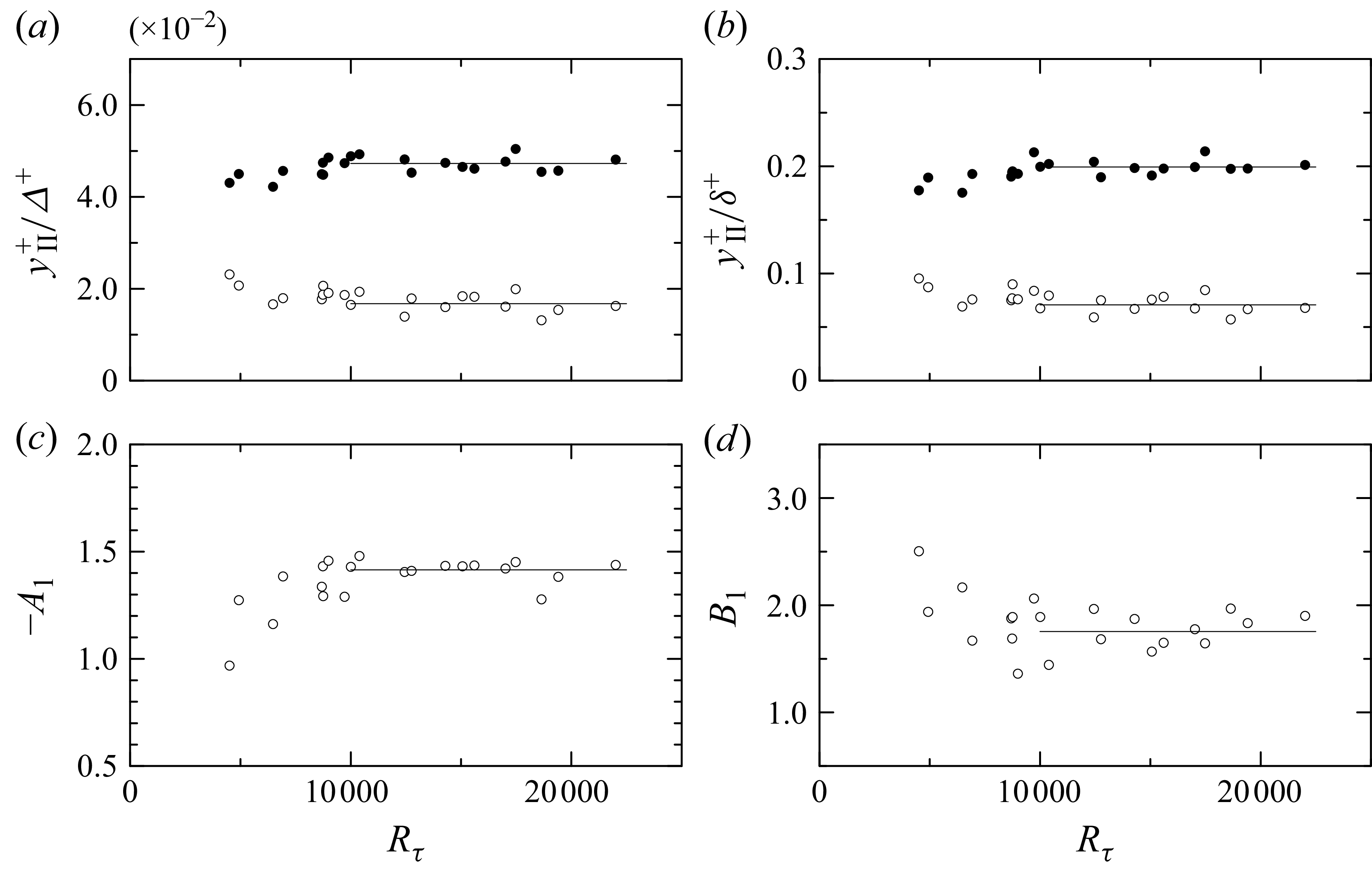
depends on Reynolds number appears to be closely related to the definition of the log-law region used to evaluate its slope, even at high Reynolds numbers. According to the self-similar concept of Townsend’s attached-eddy picture, the log-law region may be identified with the region of self-similar p.d.f.s, i.e. the invariant p.d.f. region. At high Reynolds numbers, invariant p.d.f. region II emerges and we assume that this region is appropriate for the log-law region of the attached-eddy picture. In figure 8(b), the start and end locations of invariant region II are normalised by
 $\delta$
. The ratio remains nearly constant and invariant region II can be evaluated as
 $0.07 \delta \lesssim y \lesssim 0.2 \delta$
for large Reynolds numbers (
 $R_\tau \geqslant 10^4$
). At lower Reynolds numbers, the data exhibit slight scatter because invariant region II does not appear clearly (as shown in figure 4), nor does the transient (intermediate) region. Invariant region II can also be expressed in terms of the Rotta–Clauser boundary-layer thickness as
 $0.017 \Delta \lesssim y \lesssim 0.047 \Delta$
in figure 8(a). Chauhan et al. (Reference Chauhan, Monkewitz and Nagib2009) reported that the ratio
 $\delta /\Delta$
asymptotes to
 $3.4$
as
 $R_\tau \to \infty$
, whereas the present results give
 $\delta /\Delta \simeq 4.2$
. This small discrepancy is attributed to the method of estimating the boundary-layer thickness. Chauhan et al. (Reference Chauhan, Monkewitz and Nagib2009) obtained
 $\delta$
by fitting an empirical function to the mean velocity, while in the present study,
 $\delta$
was calculated by interpolating the measurement points where
 $U(y) = 0.99 U_0$
is satisfied. In earlier work, the invariant p.d.f. region was evaluated as
 $180 \le y^+ \le 0.049 \Delta ^+$
for moderate Reynolds numbers (
 $5000 \le R_\theta \le 13\,000$
) by Tsuji et al. (Reference Tsuji, Lindgren and Johansson2005). Thus, the present outer bound of
 $0.047 \Delta ^+$
is in good agreement with the previous result.
(a) Start and end locations of invariant p.d.f. region II normalised by the Rotta–Clauser boundary-layer thickness. (b) Start and end locations of invariant p.d.f. region II normalised by the boundary-layer thickness. (c) Slope of the turbulence intensity profile,
 $A_1$
, obtained by fitting (4.4) over invariant p.d.f. region II. (d) Additive constant of the turbulence intensity profile,
 $B_1$
, obtained by fitting (4.4) over invariant p.d.f. region II.

Figure 8. Long description
The image contains four scatter plots labeled (a) through (d). Each plot shows data points representing different variables. In subplot (a), the y-axis represents the start and end locations of invariant probability density function (p.d.f.) region II normalized by the Rotta-Clauser boundary-layer thickness, while the x-axis represents the Reynolds number. Subplot (b) shows the start and end locations of invariant p.d.f. region II normalized by the boundary-layer thickness, with the same x-axis as subplot (a). Subplot (c) depicts the slope of the turbulence intensity profile, obtained by fitting a specific equation over invariant p.d.f. region II, with the y-axis labeled as negative A1 and the x-axis as the Reynolds number. Subplot (d) shows the additive constant of the turbulence intensity profile, obtained similarly, with the y-axis labeled as B1 and the same x-axis as the previous subplots. Each subplot contains several data points, with some showing clusters and others showing more scattered distributions. All values are approximated.
By fitting (4.4) to invariant p.d.f. region II, the slope
 $A_1$
and constant
 $B_1$
were calculated. The results are shown in figures 8(c) and 8(d). Both
 $A_1$
and
 $B_1$
appear to remain constant for large Reynolds numbers (
 $\textit{Re}_\tau \geqslant 10^4$
), with values of
 $A_1 \simeq 1.42$
and
 $B_1 \simeq 1.75$
. These values are slightly larger than those reported previously, but they are of the same order of magnitude. It should be emphasised that
 $A_1$
and
 $B_1$
are determined here from clearly defined regions. If the fitting region is not objectively specified, the slope and additive constant cannot be uniquely determined. In addition to the second-order moment, higher-order even moments of velocity fluctuations also exhibit logarithmic behaviour of (4.5) (
 $p$
is positive integer) and the p.d.f.s show sub-Gaussian features, as reported by Meneveau & Marusic (Reference Meneveau and Marusic2013),
 \begin{equation} \big \langle ({u}^{\prime+})^{2p} \big \rangle ^{1/p} =B_p - A_p \ln (y/\delta ). \end{equation}
The logarithmic relation of higher-order moments can be derived straightforwardly under the assumption of Gaussian p.d.f.s. However, p.d.f.s are not necessarily Gaussian. We have shown that the higher-order even moments follow the log-law distribution given in (4.5) as long as the p.d.f.s are self-similar in the considered region. The slopes are expressed as
 $A_p = (M_{2p})^{1/p} A_1, \ B_p = (M_{2p})^{1/p} B_1$
, where
 $M_{2p} = m_{2p}/m_2^p$
and
 $m_{2p}$
is the
 $2p$
th moment of the velocity fluctuations (Wada et al. Reference Wada, Furuichi, Terao and Tsuji2015; Furuichi, Ono & Tsuji Reference Furuichi, Ono and Tsuji2025). Therefore, invariant p.d.f. region II is the appropriate domain in which the log-law relation of higher-order moments, as reported by Meneveau & Marusic (Reference Meneveau and Marusic2013), is satisfied. The Townsen–Perry constant is estimated as
 $A_1 \simeq 1.42$
when fitted over invariant p.d.f. region II. However, if calculated at lower Reynolds numbers where invariant region II does not emerge, the slope exhibits Reynolds-number dependence. We suggest that previous debates on the Reynolds-number dependence of
 $A_1$
may be attributed either to the use of inappropriate fitting regions or to the relatively low Reynolds numbers employed in those evaluations.
5. Conclusions
Streamwise velocity fluctuations were measured in a zero-pressure-gradient turbulent boundary layer at high Reynolds numbers. The main findings may be summarised as follows.
When normalised by their mean and standard deviation, the probability density functions (p.d.f.s) of streamwise velocity fluctuations exhibit invariant shapes. At low Reynolds numbers, a single invariant region is observed, whereas at higher Reynolds numbers (
 $O(10^4) \lt \textit{Re}_\tau$
), an additional invariant region emerges. These invariant p.d.f. regions are located at
 $100 \lesssim y^+ \lesssim 200$
and
 $0.07 \lesssim y/\delta \lesssim 0.2$
, respectively. Within each invariant region, the p.d.f. shapes are independent of Reynolds number, indicating their universality.
The turbulent intensity profile exhibits a plateau region beyond the buffer layer, which corresponds to invariant p.d.f. region I. The plateau value, denoted by
 $\alpha$
, is closely related to the maximum turbulent intensity
 $u^+_{r,max }$
at
 $y^+ \simeq 15$
. The empirical relation,
 ${u^+_{r,max}}^2 /\alpha ^2 \simeq 5.4 R_\tau ^{-1/4} + 1.0$
given in (4.3), is proposed to predict the maximum intensity from the plateau value.
Finally, the log-law behaviour of the turbulent intensity profile was evaluated using (4.4) over invariant p.d.f. region II. The slope and additive constant were obtained as
 $A_1 \simeq 1.42$
and
 $B_1 \simeq 1.75$
, respectively, for
 $O(10^4) \lt \textit{Re}_\tau$
, and found to be independent of Reynolds number.
Acknowledgements
We would like to express our gratitude to the staff and engineers of the low-noise wind tunnel at the Railway Technical Research Institute (RTRI) for their assistance with the plate setting and wind tunnel operation. We also thank Y. Wada, K. Sakamoto and E. Kusano for their support during the measurements. Our sincere appreciation goes to Professor M. Nishioka, who guided this experiment in its early stages and provided many valuable comments. KTH data were presented by Professor A. V. Johansson and we appreciate his continous encouragement.
Funding
This work was supported in part by JSPS KAKENHI Grant Numbers JP20360083 and JP15H03923. This work is partially supported by ‘Nagoya University High Performance Computing Research Project for Joint Computational Science’ in Japan.
Declaration of interests
The authors report no conflict of interest.
Author contributions
Y.T. designed the research. Experiments were performed in the low-noise wind tunnel at the Railway Technical Research Institute (RTRI) in Maibara, Japan by Y.T. and A.I. Additionally, Y.T. contributed to data processing and interpretation, and to manuscript preparation.
Data availability statement
The data that support the findings of this study are available from the authors upon reasonable request.
Appendix A. Experimental set-up for OFI
The experimental set-up for oil-film interferometry (OFI) is shown in figure 9. A small CMOS camera (
 $1280 \times 1024$
pixels) was installed in the space between the flat plate and the wind-tunnel bottom wall. The focal distance and tilt angle
 $\alpha$
of the camera were carefully adjusted to obtain a clear fringe pattern.
(a) Schematic view of the camera arrangement for the OFI measurement. (b) Fringe pattern of the oil film and a schematic view of its cross-section.

Figure 9. Long description
The diagram on the left illustrates the setup for oil film interferometry measurement, featuring a wind tunnel, glass, sodium lamp, camera, computer, and trigger. The camera is positioned at an angle to capture the oil film. The diagram on the right shows a fringe pattern of the oil film and a schematic cross-section of the film, indicating the flow direction and the height of the oil film at different points.
The light source was a sodium lamp with a wavelength of
 $\lambda = 589.0$
nm and an area of
 $7 \,\mathrm{mm} \times 9 \,\mathrm{mm}$
was visualised. Commercial Dow Corning 200® oils (
 $50$
,
 $100$
and
 $200$
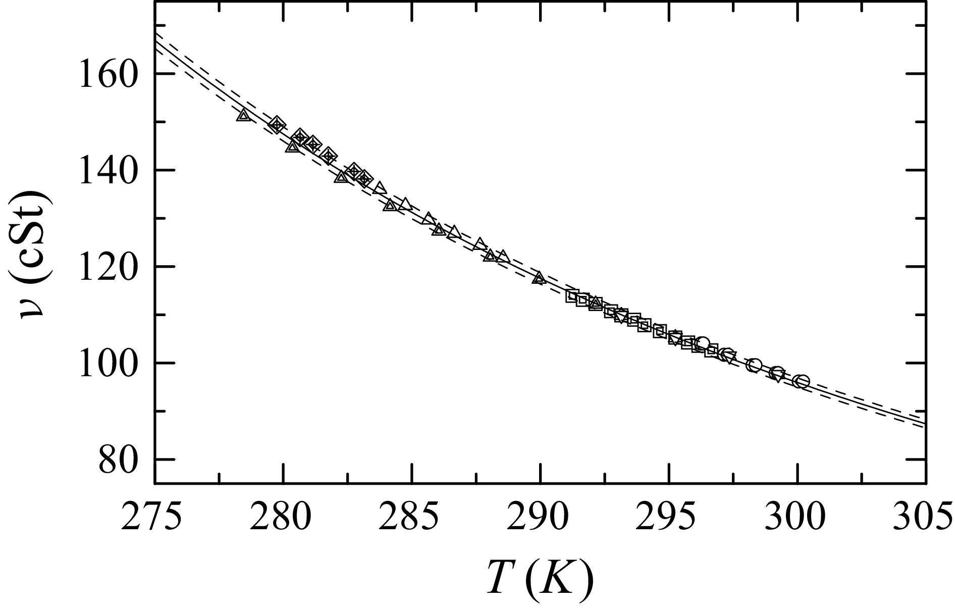
cSt), which are thermally stable and have low surface tension, were used for the measurements. The oil density was nearly constant, but its viscosity was significantly affected by temperature. Therefore, the viscosity was calibrated using an Ubbelohde viscometer immersed in a constant-temperature bath to maintain a uniform oil temperature. An empirical relation was derived to determine the viscosity at temperature
 $T$
during the measurements:
 \begin{equation} \nu = \frac {d_1}{T-d_2} + d_3, \end{equation}
where
 $d_1 = 301.5$
,
 $d_2 = 110.0$
and
 $d_3 = 0.3925$
for the nominal
 $100$
cSt oil, as shown in figure 10. The dashed lines indicate the
 $\pm 1\,\%$
uncertainty. The air temperature was monitored using a small thermistor mounted on the wall (see figure 2). The dark-fringe velocity
 $u_k$
was calculated using the relation
 \begin{equation} u_k = \frac {\textrm {d}x}{\textrm {d}t} = \frac {\tau _w h_k}{\mu }, \end{equation}
where
 $k$
is the index of the dark fringe counted from the leading edge and
 $h_k$
is the thickness of the oil film. The wall shear stress is given by
 \begin{equation} \tau _w = \rho \nu u_k \frac {2\sqrt {n^2 - \sin ^2 \alpha }}{\lambda (k + h_0/\Delta h)}, \end{equation}
where
 $\nu$
is the kinematic viscosity,
 $\mu$
is viscosity and
 $\rho$
is density of oil (
 $\nu = \mu /\rho$
),
 $\Delta h = h_k - h_{k-1}$
,
 $n$
is the refractive index of the oil,
 $\lambda$
is the illumination wavelength (
 $589.0$
nm) and
 $\alpha$
is the camera angle. This procedure is referred to as the X-T method. When the bright or dark intensities of the interference fringes are fitted by trigonometric functions, a local wavelength
 $\lambda _k$
around the
 $k$
th fringe can be determined as
 \begin{equation} \frac {\textrm {d} \lambda _k}{\textrm {d}t} = u_k - u_{k-1} = \frac {\tau _w}{\mu }(h_k - h_{k-1}) = \frac {\tau _w}{\mu } \Delta h, \end{equation}
from which the wall shear stress can be obtained as
 \begin{equation} \tau _w = \frac {\mu }{\Delta h} \frac {\textrm {d} \lambda _k} {\textrm {d}t} = \rho \nu \frac {\textrm {d} \lambda _k}{\textrm {d}t} \frac {2\sqrt {n^2 - \sin ^2 \alpha }}{\lambda }. \end{equation}
Dependence of oil viscosity on temperature for the nominal 100 cSt oil. Different symbols indicate independent measurements.

Figure 10. Long description
The line graph illustrates the dependence of oil viscosity on temperature for the nominal 100 centistokes oil. The x-axis represents temperature in Kelvin, ranging from 275 to 305 Kelvin. The y-axis represents viscosity in centistokes, ranging from 80 to 160 centistokes. Different symbols such as triangles, squares, and circles indicate independent measurements. The data points show a downward trend, indicating that as the temperature increases, the viscosity of the oil decreases. The solid black line represents a formula derived from the finite-dissipation assumption, while the green line corresponds to the attached-eddy model. Both lines exhibit similar trends, making it difficult to distinguish between them. The graph shows that the present experimental values are smaller than the empirical relations reported by previous studies, likely due to the spatial-resolution limitation of the hot-wire probe. All values are approximated.
This approach is referred to as the
 $\lambda$
-method. Both (A3) and (A5) yield, in principle, the same shear stress when an appropriate fringe index
 $k$
is selected. In practice, both methods were applied and the wall shear stress was taken as the common value when the two results were in agreement. The resulting skin-friction coefficient is plotted in figure 3.


 U0
 uτ
 Rθ
 θ
 Rθ=U0θ/ν
 ν
 Rτ
 δ
 Rτ=uτδ/ν
 δ
 0.99U0
 Δ+
 ℓ+

 400
 △
 x=6.0
 λ
 ◻
 x=14.4
 λ
 ∘
 x=18.7
 λ
 ▴
 x=6.0
 XT
 ◼
 x=14.4
 XT
 ∙
 x=18.7
 XT
 κ=0.384
 C=3.1
 ±1%
 κ=0.40
 C=4.3
 Rδ∗
 uτΔ/ν

 Reτ=2130
 d=2.5
 μ
 ℓ+
 Reτ=6935
 Reτ=15070
 U+=(1/κ)ln(y+)+B
 κ=0.384
 B=4.17

 △
 Reτ=6935
 ×
 Reτ=15070
 ∙
 ℓ+⩽26.0
 ∘
 ℓ+>26.0
 ⊚
 x=5.5
 ℓ+⩽25.0
 ⊡
 Rτ=18000
 ×
 ur,max+=[11.5−19.3Rτ−1/4]1/2
 ur,max+=[3.54+0.646ln(Rτ)]1/2
 α
 ur,max+
 α=[10.73−47.35Rτ−1/4]1/2
 α=[22−470/U0+]1/2
 α=0.33Reθ0.21
 α2
 ∙
 ℓ+⩽26.0
 ∘
 ℓ+>26.0
 ⊚
 x=5.5
 ⊡
 Rτ=18000
 ×
 (ur,max+)2/α2=5.4Rτ−1/4+1.0
 (ur,max+)2/α2=(22−340/U0+)/(22−470/U0+)
 A1
 B1