





1 Introduction
Beyond a critical flow rate such that the ratio of the inertial force to the viscous force is large enough, inertial instabilities can often be observed in Newtonian fluid flows. In recent decades, an increased attention has been placed on trying to understand, and use, such phenomena in mixing processes and other industrial applications. Pioneering work relating to inertial instabilities was undertaken by Reynolds (Reference Reynolds1883) in pipe flow. For many decades after this insight of Reynolds regarding such instabilities, scientists were not able to successfully predict the onset of the instability in a pipe. Today, we know this difficulty is related to the nonlinear form of the instability, and pipe flow still remains an outstanding challenge and the subject of many current studies (Eckhardt et al. Reference Eckhardt, Schneider, Hof and Westerweel2007; Eckhardt Reference Eckhardt2009; Mullin Reference Mullin2011).
Taylor (Reference Taylor1923), following on from the works by Couette (Reference Couette1888) and Mallock (Reference Mallock1888), who used concentric-cylinder devices for viscometric purposes, was the first researcher who suggested to study inertial instabilities in the concentric-cylinder geometry. In this paper, Taylor was able, by using a linear stability analysis, to successfully predict the onset of secondary flow (so-called ‘Taylor vortices’) in excellent agreement with experiments. In recognition of this advancement, the concentric-cylinder geometry is now often called ‘Taylor–Couette’ (TC) flow (Mallock’s important contribution being somewhat overlooked). Since these early works, this geometry has received such a great deal of attention from researchers that this geometry has been referred to as the ‘hydrogen atom of fluid dynamics’ (Tagg Reference Tagg1994; Fardin, Perge & Taberlet Reference Fardin, Perge and Taberlet2014). The TC geometry has several advantages over the pipe. First of all, in the small-gap limit, the shear rate is constant across the gap (
 $\dot{\tilde{\unicode[STIX]{x1D6FE}}}=(|\tilde{\unicode[STIX]{x1D714}}-\tilde{\unicode[STIX]{x1D714}}_{o}|\tilde{R}_{i})/2\tilde{a}$
, where
 $\tilde{\unicode[STIX]{x1D714}}$
and
 $\tilde{\unicode[STIX]{x1D714}}_{o}$
are the dimensional rotation speeds of the inner and outer walls and
 $\tilde{R}_{i}$
and
 $2\tilde{a}$
are the radius of the inner cylinder and the gap between the two cylinders, respectively). Secondly, streamlines are curved. Thirdly, the nature of the instability in this geometry is linear, so it could be dealt with much easier than pipe flow. Upon eliminating the effect of confining walls on the top and the bottom of the TC geometry, and assuming axisymmetry, i.e. one-dimensional (1D) flow assumption, the fluid must have a rectilinear velocity distribution with no secondary flow. Taylor showed that, beyond a critical rotation speed, by adding a small perturbation, a nonlinear distribution of the main flow field with pairs of steady secondary flows replaces the previous rectilinear distribution. Nowadays the TC geometry is considered a benchmark geometry in the fluid mechanics community, and devices with different aspect ratio (height/gap)
 $\unicode[STIX]{x1D6EC}$
(ranging from as small as 0.2) have been used for various purposes (Muller, Larson & Shaqfeh Reference Muller, Larson and Shaqfeh1989; Berret, Porte & Decruppe Reference Berret, Porte and Decruppe1997; Lerouge, Decruppe & Berret Reference Lerouge, Decruppe and Berret2000; Mullin, Toya & Tavener Reference Mullin, Toya and Tavener2002; Hu & Lips Reference Hu and Lips2005; Lee et al.
Reference Lee, Fuller, Hudson and Yuan2005; Liberatore et al.
Reference Liberatore, Nettesheim, Wagner and Porcar2006; Gurnon et al.
Reference Gurnon, Lopez-Barron, Eberle, Porcar and Wagner2014; López-Barrón, Wagner & Porcar Reference López-Barrón, Wagner and Porcar2015). For example, TC cells with aspect ratios
 $3<\unicode[STIX]{x1D6EC}<12$
are commonly used for both small-angle neutron scattering (Hu & Lips Reference Hu and Lips2005; Liberatore et al.
Reference Liberatore, Nettesheim, Wagner and Porcar2006; Gurnon et al.
Reference Gurnon, Lopez-Barron, Eberle, Porcar and Wagner2014; López-Barrón et al.
Reference López-Barrón, Wagner and Porcar2015) and flow birefringence experiments (Muller et al.
Reference Muller, Larson and Shaqfeh1989; Berret et al.
Reference Berret, Porte and Decruppe1997; Lerouge et al.
Reference Lerouge, Decruppe and Berret2000; Mullin et al.
Reference Mullin, Toya and Tavener2002; Lee et al.
Reference Lee, Fuller, Hudson and Yuan2005).
The confining effect of walls on the stability and bifurcation of Newtonian fluids in inertial regimes was studied by Benjamin (Reference Benjamin1978a ) using the existence theory due originally to Leray & Schauder (Reference Leray and Schauder1934). Benjamin (Reference Benjamin1978a ) concluded that the supercritical nature of the instability, which was previously reported by Taylor (Reference Taylor1923) based on an idealized 1D assumption for the base state, will not typically be observed in a physical flow between two finite concentric cylinders. Following this argument, a different process whereby the primary flow undergoes ‘morphogenesis’ was predicted by including the effect of the walls on the top and bottom of the geometry. In a following experimental study (Benjamin Reference Benjamin1978b ), support for the theoretical part was provided showing a decoupling of the supercritical bifurcation for finite-aspect-ratio TC geometries. The results clearly showed that, once the inner cylinder starts to rotate from the stationary state, a secondary motion appears, which gets more intensified with increasing Reynolds number. Similar qualitative results were obtained in a numerical study by De Roquefort & Grillaud (Reference De Roquefort and Grillaud1978) and a theoretical analysis by Schaeffer (Reference Schaeffer1980), which used a homotopy approach to include the physically realistic effect of the fixed wall on the end faces of the cylinders.
Görtler (Reference Görtler1944), in later research, showed that most of the criteria for TC instability can be directly compared with more general curved boundary-layer flow. The main difference between flow in curved boundary layers and TC flow is related to the fact that in the TC system the fluid experiences a wall-driven motion while in curved ducts or curved boundary layers it is usually pressure-driven. Seminal papers by Dean (Reference Dean1927, Reference Dean1928) tried to capture the structure of Taylor–Görtler vortices in curved pipes, which were previously studied experimentally by Eustice (Reference Eustice1911). Dean (Reference Dean1927, Reference Dean1928) implemented a perturbation method, using the ratio of the pipe radius over the curvature radius as the perturbation parameter for the pressure-driven flow inside a curved pipe. Owing to the presence of centrifugal forces, pressure gradients in the lateral directions of the pipe appear, stimulating a pair of steady secondary vortices. In this case, the centrifugal force causes fluid particles to move from the inner side of the curvature towards the outer side, while conservation of mass requires a replacement of particles and consequently a pair of secondary flow vortices appear. A similar method by Winters (Reference Winters1987) extended the analysis to flow in curved rectangular ducts. Thus, it is now well known that the combination of inertia and curvature leads to secondary flow for Newtonian fluids.
In contrast, for viscoelastic fluids a secondary flow develops even in the inertialess limit for the curved pipe geometry, and such studies have received a great deal of attention because of their applications in mixing and other systems (Akiyama & Cheng Reference Akiyama and Cheng1974; Finlay Reference Finlay1989; Kumar, Aggarwal & Nigam Reference Kumar, Aggarwal and Nigam2006; Ali et al. Reference Ali, Sajid, Abbas and Javed2010; Keshavarz-Motamed & Kadem Reference Keshavarz-Motamed and Kadem2011; Hayat, Noreen & Alsaedi Reference Hayat, Noreen and Alsaedi2012; Hoque et al. Reference Hoque, Alam, Ferdows and Bég2013). Fan, Tanner & Phan-Thien (Reference Fan, Tanner and Phan-Thien2001), based on an order-of-magnitude analysis, derived an equation for the Oldroyd-B model in such curved pipe flows, showing a correlation between the so-called ‘hoop’ stress (the normal stress in the azimuthal direction) and centrifugal force. They show that fluid inertia and hoop stress are two significant and competitive forces near the core region, which contribute to establishing a pressure gradient and consequently the presence of secondary flow. Poole, Lindner & Alves (Reference Poole, Lindner and Alves2013), in a numerical simulation, showed that for creeping flow of a viscoelastic fluid in ‘serpentine’ channels a pair of secondary flow vortices exists that is absent for the equivalent inertialess Newtonian flow. These secondary flows can be attributed to the effect of curvature and elastic normal stress similar to the Dean flow structure except that in the viscoelastic case there is no inertia. Within a similar context, Robertson & Muller (Reference Robertson and Muller1996) and Jitchote & Robertson (Reference Jitchote and Robertson2000) captured combined effects of elastic force and centrifugal force in curved pipes. In these papers, similar to the previous works by Dean (Reference Dean1927, Reference Dean1928), a perturbation method was employed to show that, even in the absence of inertia, elastic normal stresses are able to create hoop stresses and generate secondary flows.
In the last 25 years, research into complex viscoelastic fluids has highlighted that, even in the absence of inertial forces (i.e. creeping flow), similar mechanisms to inertial instabilities can be generated solely due to the nonlinear elastic forces; such instabilities are called ‘purely elastic’ (Shaqfeh Reference Shaqfeh1996). The flow between two concentric cylinders (TC flow described above) has routinely been studied by researchers in viscoelastic fluids due to its wide range of applications especially in rheometry (Mallock Reference Mallock1888; Taylor Reference Taylor1923). Following the studies already discussed on the effect of inertial instabilities in the TC system and Dean flows (Dean Reference Dean1928), a number of researchers tried to extend this scenario to the case of viscoelastic fluids. The modifying effects of viscoelasticity on the inertial TC instabilities were investigated by Giesekus (Reference Giesekus1966, Reference Giesekus1972) both experimentally and analytically using the second-order fluid model. Generally, a second-order fluid is the lowest-order form of a mathematical constitutive equation after the Newtonian fluid (first-order solution) so is only suitable for simulation of slow and slowly varying flow, while in the case of purely viscoelastic instabilities, driven by nonlinear effects, this assumption is not strictly valid (Bird et al. Reference Bird, Armstrong, Hassager and Curtiss1977). Muller et al. (Reference Muller, Larson and Shaqfeh1989) showed experimentally that, in the absence of significant second normal-stress differences, using a Boger fluid, a purely elastic instability can be observed. They showed that, unlike the steady nature of TC vortices, in the purely elastic case the structure has an oscillatory form the wavelength of which decreases with time. From these seminal results, it can be deduced that the first normal-stress difference should play a key role in purely elastic instabilities. An up-to-date review on viscoelastic flows in the TC system and different types of instabilities can be found in Muller (Reference Muller2008). A theoretical study to estimate the onset conditions of purely elastic instabilities was carried out by Larson, Shaqfeh & Muller (Reference Larson, Shaqfeh and Muller1990). Using a linear stability analysis, they employed a perturbation method to predict the threshold of this instability. Larson et al. (Reference Larson, Shaqfeh and Muller1990) eliminated the effect of confining walls on the top and bottom of the geometry, and disturbed an initially 1D axisymmetric flow using a time-periodic function and showed that only after a critical shear rate did an instability in the form of a time-dependent secondary flow occur, in qualitative agreement with experiments of Muller et al. (Reference Muller, Larson and Shaqfeh1989).
The previous studies for viscoelastic fluids suggested that the presence of secondary flows was only attributed to the onset of a purely elastic instability in the TC geometry (Giesekus Reference Giesekus1966, Reference Giesekus1972; Muller et al. Reference Muller, Larson and Shaqfeh1989; Larson et al. Reference Larson, Shaqfeh and Muller1990). In this work it will be shown that, by considering the effect of confining walls, even before the onset of any potential purely elastic instability, a pair of steady secondary vortices exists in the region near the corner of the moving wall and the stationary wall. Indeed, viscoelastic flow through finite-aspect-ratio curved ducts is characterized by secondary flows which are driven by a combination of curvature and stress gradients near the duct walls that significantly affect the primary flow. Although never previously studied, in a TC system this issue is likely to play an important role in both the base-state solutions and the purely elastic instability threshold of viscoelastic fluids in the TC system, especially for shallow geometries (i.e. small aspect ratios). In this study we attempt to fill this gap by investigating finite end effects for the narrow-gap concentric-cylinder geometry under inertialess conditions for viscoelastic fluids using both an approximate analytical perturbation approach, full nonlinear simulations with the Oldroyd-B model and supporting experiments.
2 Mathematical formulation
In this section the mathematical formulation for creeping viscoelastic TC flow is presented. Here, the problem is investigated for the particular case that the inner cylinder is rotating while the other three surfaces (i.e. the other cylinder and the two end faces) are stationary. To probe the viscoelastic behaviour, the Oldroyd-B model is chosen, as this is the simplest differential constitutive equation capable of predicting many complex phenomena due to viscoelasticity (Alves & Poole Reference Alves and Poole2007; Poole, Alves & Oliveira Reference Poole, Alves and Oliveira2007).
2.1 Coordinate system
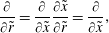
In this work, symbols with and without tildes denote dimensional and non-dimensional parameters, respectively. Considering the geometry of the problem, a cylindrical polar coordinate system is used (figure 1). Introducing the following change of variable, one can write
 $$\begin{eqnarray}\displaystyle & \displaystyle \tilde{x}=\tilde{r}-\tilde{R}, & \displaystyle\end{eqnarray}$$
 $$\begin{eqnarray}\displaystyle & \displaystyle \frac{1}{\tilde{r}}=\frac{1}{\tilde{x}+\tilde{R}}, & \displaystyle\end{eqnarray}$$
 $$\begin{eqnarray}\displaystyle & \displaystyle \frac{\unicode[STIX]{x2202}}{\unicode[STIX]{x2202}\tilde{r}}=\frac{\unicode[STIX]{x2202}}{\unicode[STIX]{x2202}\tilde{x}}\frac{\unicode[STIX]{x2202}\tilde{x}}{\unicode[STIX]{x2202}\tilde{r}}=\frac{\unicode[STIX]{x2202}}{\unicode[STIX]{x2202}\tilde{x}}, & \displaystyle\end{eqnarray}$$
where
 $\tilde{R}$
is the mid radius (
 $\tilde{R}=\tilde{R}_{i}+\tilde{a}$
, with
 $\tilde{R}_{i}$
and
 $\tilde{a}$
the radius of the inner cylinder and the half-width of the gap, respectively) and
 $\tilde{r},~\unicode[STIX]{x1D703},~\tilde{z}$
are the components of the polar cylindrical coordinate system.
Schematic of the narrow-gap TC set-up investigated including polar cylindrical coordinate system: (a) concentric-cylinder set-up; and (b) axisymmetric ‘slice’ used in analytical method.

2.2 Non-dimensionalization
It is convenient to use dimensionless parameters in this problem. The relationships between dimensional and dimensionless parameters are
 $$\begin{eqnarray}\left.\begin{array}{@{}c@{}}\displaystyle x=\frac{\tilde{x}}{\tilde{a}},\quad z=\frac{\tilde{z}}{\tilde{a}\unicode[STIX]{x1D6EC}},\quad \unicode[STIX]{x1D6EC}=\frac{\tilde{b}}{\tilde{a}},\quad \unicode[STIX]{x1D6FD}=\frac{\tilde{\unicode[STIX]{x1D702}}_{s}}{\tilde{\unicode[STIX]{x1D702}}},\quad Wi=\frac{\tilde{\unicode[STIX]{x1D706}}\tilde{R}_{i}\tilde{\unicode[STIX]{x1D714}}}{\tilde{a}},\quad \unicode[STIX]{x1D749}=\frac{\tilde{\unicode[STIX]{x1D749}}\tilde{a}}{\tilde{\unicode[STIX]{x1D702}}\tilde{R}_{i}\tilde{\unicode[STIX]{x1D714}}},\quad P=\frac{\tilde{P}\tilde{a}}{\tilde{\unicode[STIX]{x1D702}}\tilde{R}_{i}\tilde{\unicode[STIX]{x1D714}}},\\ \displaystyle v_{r}=\frac{\tilde{v}_{r}}{\tilde{R}_{i}\tilde{\unicode[STIX]{x1D714}}},\quad v_{\unicode[STIX]{x1D703}}=\frac{\tilde{v}_{\unicode[STIX]{x1D703}}}{\tilde{R}_{i}\tilde{\unicode[STIX]{x1D714}}},\quad v_{z}=\frac{\tilde{v}_{z}}{\tilde{R}_{i}\tilde{\unicode[STIX]{x1D714}}},\quad \unicode[STIX]{x1D63F}=\frac{\tilde{\unicode[STIX]{x1D63F}}\tilde{a}}{\tilde{R}_{i}\tilde{\unicode[STIX]{x1D714}}},\quad \unicode[STIX]{x1D6FF}=\frac{\tilde{a}}{\tilde{R}},\quad B=1+\unicode[STIX]{x1D6FF}x,\end{array}\right\}\end{eqnarray}$$
where
 $\tilde{x}$
is the variable defined in (2.1),
 $\tilde{z}$
is the axial variable in the polar cylindrical coordinate system,
 $\tilde{b}$
is the half-height of the cylinders,
 $\unicode[STIX]{x1D6EC}$
is the aspect ratio,
 $\unicode[STIX]{x1D6FD}$
is the solvent to total viscosity ratio,
 $\tilde{\unicode[STIX]{x1D702}}$
is the total viscosity of the fluid (
 $\tilde{\unicode[STIX]{x1D702}}=\tilde{\unicode[STIX]{x1D702}}_{p}+\tilde{\unicode[STIX]{x1D702}}_{s}$
, with
 $\tilde{\unicode[STIX]{x1D702}}_{p}$
and
 $\tilde{\unicode[STIX]{x1D702}}_{s}$
the polymeric and solvent parts of the viscosity, respectively),
 $Wi$
is the Weissenberg number,
 $\tilde{\unicode[STIX]{x1D706}}$
is the corresponding relaxation time of the fluid,
 $\tilde{\unicode[STIX]{x1D714}}$
is the angular velocity of the moving inner wall,
 $\tilde{\unicode[STIX]{x1D749}}$
is the stress tensor,
 $\tilde{P}$
is the pressure,
 $\tilde{\boldsymbol{U}}$
is the velocity vector,
 $\tilde{v}_{r},~\tilde{v}_{\unicode[STIX]{x1D703}}$
and
 $\tilde{v}_{z}$
are components in the
 $\tilde{r}$
,
 $\unicode[STIX]{x1D703}$
and
 $\tilde{z}$
directions of velocity in the polar cylindrical coordinate system and
 $\tilde{\unicode[STIX]{x1D63F}}$
is the rate-of-deformation tensor
 $(\tilde{\unicode[STIX]{x1D63F}}=(\unicode[STIX]{x1D735}\tilde{\boldsymbol{U}}+\unicode[STIX]{x1D735}\tilde{\boldsymbol{U}}^{\text{T}})/2)$
. Finally,
 $\unicode[STIX]{x1D6FF}$
is the curvature ratio and
 $B$
represents the local dimensionless curvature.
2.3 Constitutive equation
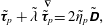
To simulate the viscoelastic behaviour, the Oldroyd-B constitutive equation is used to calculate the stress components. This model considers a Newtonian behaviour for the solvent contribution (
 $\tilde{\unicode[STIX]{x1D749}}_{s}$
) of the fluid and an upper convected Maxwell model for the polymeric part (
 $\tilde{\unicode[STIX]{x1D749}}_{p}$
) of the stress tensor. The constitutive equation is then (Robertson & Muller Reference Robertson and Muller1996):
 $$\begin{eqnarray}\displaystyle & \displaystyle \tilde{\unicode[STIX]{x1D749}}=\tilde{\unicode[STIX]{x1D749}}_{s}+\tilde{\unicode[STIX]{x1D749}}_{p}, & \displaystyle\end{eqnarray}$$
 $$\begin{eqnarray}\displaystyle & \displaystyle \tilde{\unicode[STIX]{x1D749}}_{s}=2\tilde{\unicode[STIX]{x1D702}}_{s}\,\tilde{\unicode[STIX]{x1D63F}}, & \displaystyle\end{eqnarray}$$
 $$\begin{eqnarray}\displaystyle & \displaystyle \tilde{\unicode[STIX]{x1D749}}_{p}+\tilde{\unicode[STIX]{x1D706}}\stackrel{\unicode[STIX]{x1D735}}{\tilde{\unicode[STIX]{x1D749}}_{p}}=2\tilde{\unicode[STIX]{x1D702}}_{p}\tilde{\unicode[STIX]{x1D63F}}, & \displaystyle\end{eqnarray}$$
 $\stackrel{\unicode[STIX]{x1D735}}{\tilde{\unicode[STIX]{x1D749}}_{p}}$
is defined as (Bird et al.
Reference Bird, Armstrong, Hassager and Curtiss1977):
 $$\begin{eqnarray}\stackrel{\unicode[STIX]{x1D735}}{\tilde{\unicode[STIX]{x1D749}}_{p}}=\left(\frac{\unicode[STIX]{x2202}}{\unicode[STIX]{x2202}\tilde{t}}+\tilde{\boldsymbol{U}}\boldsymbol{\cdot }\unicode[STIX]{x1D735}\right)\tilde{\unicode[STIX]{x1D749}}_{p}-\{(\unicode[STIX]{x1D735}\tilde{\boldsymbol{U}}^{\text{T}})(\tilde{\unicode[STIX]{x1D749}}_{p})+(\tilde{\unicode[STIX]{x1D749}}_{p})(\unicode[STIX]{x1D735}\tilde{\boldsymbol{U}})\}.\end{eqnarray}$$
3 Analytical methods
3.1 Governing equations
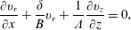
The governing equations in this problem are conservation of mass and momentum. These equations using the change of variable defined in (2.1) in a polar cylindrical coordinate system assuming axisymmetry and creeping flow (i.e.
 $Re\rightarrow 0$
) can be presented in dimensionless form as follows:
 $$\begin{eqnarray}\frac{\unicode[STIX]{x2202}v_{r}}{\unicode[STIX]{x2202}x}+\frac{\unicode[STIX]{x1D6FF}}{B}v_{r}+\frac{1}{\unicode[STIX]{x1D6EC}}\frac{\unicode[STIX]{x2202}v_{z}}{\unicode[STIX]{x2202}z}=0,\end{eqnarray}$$
 $$\begin{eqnarray}\displaystyle & & \displaystyle -\frac{\unicode[STIX]{x2202}P}{\unicode[STIX]{x2202}x}+\unicode[STIX]{x1D6FD}\left(\frac{\unicode[STIX]{x2202}^{2}v_{r}}{\unicode[STIX]{x2202}x^{2}}+\frac{\unicode[STIX]{x1D6FF}}{B}\frac{\unicode[STIX]{x2202}v_{r}}{\unicode[STIX]{x2202}x}-\frac{\unicode[STIX]{x1D6FF}^{2}}{B^{2}}v_{r}+\frac{1}{\unicode[STIX]{x1D6EC}^{2}}\frac{\unicode[STIX]{x2202}^{2}v_{r}}{\unicode[STIX]{x2202}z^{2}}\right)+\frac{\unicode[STIX]{x2202}\unicode[STIX]{x1D70F}_{p,rr}}{\unicode[STIX]{x2202}x}+\frac{\unicode[STIX]{x1D6FF}}{B}(\unicode[STIX]{x1D70F}_{p,rr}-\unicode[STIX]{x1D70F}_{p,\unicode[STIX]{x1D703}\unicode[STIX]{x1D703}})\nonumber\\ \displaystyle & & \displaystyle \quad +\,\frac{1}{\unicode[STIX]{x1D6EC}}\frac{\unicode[STIX]{x2202}\unicode[STIX]{x1D70F}_{p,rz}}{\unicode[STIX]{x2202}z}=0,\end{eqnarray}$$
 $$\begin{eqnarray}\displaystyle & \displaystyle \unicode[STIX]{x1D6FD}\left(\frac{\unicode[STIX]{x2202}^{2}v_{\unicode[STIX]{x1D703}}}{\unicode[STIX]{x2202}x^{2}}+\frac{\unicode[STIX]{x1D6FF}}{B}\frac{\unicode[STIX]{x2202}v_{\unicode[STIX]{x1D703}}}{\unicode[STIX]{x2202}x}-\frac{\unicode[STIX]{x1D6FF}^{2}}{B^{2}}v_{\unicode[STIX]{x1D703}}+\frac{1}{\unicode[STIX]{x1D6EC}^{2}}\frac{\unicode[STIX]{x2202}^{2}v_{\unicode[STIX]{x1D703}}}{\unicode[STIX]{x2202}z^{2}}\right)+\frac{\unicode[STIX]{x2202}\unicode[STIX]{x1D70F}_{p,r\unicode[STIX]{x1D703}}}{\unicode[STIX]{x2202}x}+\frac{2\unicode[STIX]{x1D6FF}}{B}\unicode[STIX]{x1D70F}_{p,r\unicode[STIX]{x1D703}}+\frac{1}{\unicode[STIX]{x1D6EC}}\frac{\unicode[STIX]{x2202}\unicode[STIX]{x1D70F}_{p,\unicode[STIX]{x1D703}z}}{\unicode[STIX]{x2202}z}=0,\qquad & \displaystyle\end{eqnarray}$$
 $$\begin{eqnarray}\displaystyle & \displaystyle -\frac{1}{\unicode[STIX]{x1D6EC}}\frac{\unicode[STIX]{x2202}P}{\unicode[STIX]{x2202}z}+\unicode[STIX]{x1D6FD}\left(\frac{\unicode[STIX]{x2202}^{2}v_{z}}{\unicode[STIX]{x2202}x^{2}}+\frac{\unicode[STIX]{x1D6FF}}{B}\frac{\unicode[STIX]{x2202}v_{z}}{\unicode[STIX]{x2202}x}+\frac{1}{\unicode[STIX]{x1D6EC}^{2}}\frac{\unicode[STIX]{x2202}^{2}v_{z}}{\unicode[STIX]{x2202}z^{2}}\right)+\frac{\unicode[STIX]{x2202}\unicode[STIX]{x1D70F}_{p,rz}}{\unicode[STIX]{x2202}x}+\frac{\unicode[STIX]{x1D6FF}}{B}\unicode[STIX]{x1D70F}_{p,rz}+\frac{1}{\unicode[STIX]{x1D6EC}}\frac{\unicode[STIX]{x2202}\unicode[STIX]{x1D70F}_{p,zz}}{\unicode[STIX]{x2202}z}=0.\qquad & \displaystyle\end{eqnarray}$$
As TC flow is a wall-driven problem, there is no pressure gradient in the
 $\unicode[STIX]{x1D703}$
direction. However, the presence of the secondary flow causes a pressure distribution in both the
 $r$
and
 $z$
directions (see (3.2a
) and (3.2c
)) that is an unknown function of
 $x$
,
 $z$
and of the rheological parameters. It is usual to eliminate the pressure gradient in the equations (Robertson & Muller Reference Robertson and Muller1996; Jitchote & Robertson Reference Jitchote and Robertson2000). To achieve this, the derivative of (3.2a
) with respect to
 $z$
can be subtracted from the product of
 $\unicode[STIX]{x1D6EC}$
and the derivative of (3.2c
) with respect to
 $x$
.
3.2 Mathematical modelling
In this section the mathematical methods used to derive an approximate analytical solution to the creeping flow of viscoelastic fluids in the narrow-gap TC system are presented. The employed Oldroyd-B model is classified as a quasi-linear equation (Bird et al. Reference Bird, Armstrong, Hassager and Curtiss1977); in order to linearize this constitutive equation, a perturbation method is employed. Finally, to cope with the partial differential form of the equations, a separation-of-variables method is used to transform the problem into two linear ordinary differential equations (Myint-U & Debnath Reference Myint-U and Debnath2007; Norouzi & Biglari Reference Norouzi and Biglari2013).
3.2.1 Exact solution for finite-aspect-ratio planar Couette flow
In the case that
 $\unicode[STIX]{x1D6FF}=0$
, (3.1) and (3.2) represent the conservation of mass and momentum in a rectangular coordinate system. For the particular case of Newtonian planar Couette flow (i.e.
 $\unicode[STIX]{x1D6FF}=0$
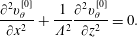
and polymer stress terms equal to zero) – which from herein onwards we will denote using a zero superscript inside square brackets (i.e. [0]) – due to the rectilinear distribution of velocity (i.e. no secondary motions in either radial or axial directions;
 $v_{r}^{[0]}=v_{z}^{[0]}=0$
), the momentum equation can be simplified to
 $$\begin{eqnarray}\frac{\unicode[STIX]{x2202}^{2}v_{\unicode[STIX]{x1D703}}^{[0]}}{\unicode[STIX]{x2202}x^{2}}+\frac{1}{\unicode[STIX]{x1D6EC}^{2}}\frac{\unicode[STIX]{x2202}^{2}v_{\unicode[STIX]{x1D703}}^{[0]}}{\unicode[STIX]{x2202}z^{2}}=0.\end{eqnarray}$$
Considering the change of variable introduced in (2.1), equation (3.3) should be solved subject to the following boundary conditions at the walls:
 $$\begin{eqnarray}\displaystyle & \displaystyle v_{\unicode[STIX]{x1D703}}^{[0]}|_{x=1}=v_{\unicode[STIX]{x1D703}}^{[0]}|_{z=1}=v_{\unicode[STIX]{x1D703}}^{[0]}|_{z=-1}=0, & \displaystyle\end{eqnarray}$$
 $$\begin{eqnarray}\displaystyle & \displaystyle v_{\unicode[STIX]{x1D703}}^{[0]}|_{x=-1}=1. & \displaystyle\end{eqnarray}$$
Equation (3.3) is a linear partial differential equation. To solve it, a separation-of-variables method can be used. The velocity may be written as
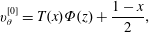 $$\begin{eqnarray}v_{\unicode[STIX]{x1D703}}^{[0]}=T(x)\unicode[STIX]{x1D6F7}(z)+\frac{1-x}{2},\end{eqnarray}$$
where the second term on the right-hand side of (3.5) solves the equation (3.3) when
 $\unicode[STIX]{x1D6EC}\rightarrow \infty$
and is the solution to the 1D case. Using the above definition (3.5), equation (3.3) can be rewritten as two linear ordinary differential equations:
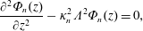 $$\begin{eqnarray}\displaystyle & \displaystyle \frac{\unicode[STIX]{x2202}^{2}\unicode[STIX]{x1D6F7}_{n}(z)}{\unicode[STIX]{x2202}z^{2}}-\unicode[STIX]{x1D705}_{n}^{2}\unicode[STIX]{x1D6EC}^{2}\unicode[STIX]{x1D6F7}_{n}(z)=0, & \displaystyle\end{eqnarray}$$
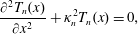 $$\begin{eqnarray}\displaystyle & \displaystyle \frac{\unicode[STIX]{x2202}^{2}T_{n}(x)}{\unicode[STIX]{x2202}x^{2}}+\unicode[STIX]{x1D705}_{n}^{2}T_{n}(x)=0, & \displaystyle\end{eqnarray}$$
where
 $\unicode[STIX]{x1D705}_{n}$
are unknown eigenvalues. The solutions to (3.6) and (3.7) are obtained as follows:
 $$\begin{eqnarray}\displaystyle & \displaystyle \unicode[STIX]{x1D6F7}_{n}(z)=A_{n}\sinh (\unicode[STIX]{x1D705}_{n}\unicode[STIX]{x1D6EC}z)+B_{n}\cosh (\unicode[STIX]{x1D705}_{n}\unicode[STIX]{x1D6EC}z), & \displaystyle\end{eqnarray}$$
 $$\begin{eqnarray}\displaystyle & \displaystyle T_{n}(x)=C_{n}\sin (\unicode[STIX]{x1D705}_{n}x)+D_{n}\cos (\unicode[STIX]{x1D705}_{n}x). & \displaystyle\end{eqnarray}$$
The solution to equation (3.9) should be solved subject to
 $T_{n}(x)|_{x=1}=0$
, hence
 $D_{n}=-C_{n}\tan (\unicode[STIX]{x1D705}_{n})$
, so
 $$\begin{eqnarray}T_{n}(x)=E_{n}(\cos (\unicode[STIX]{x1D705}_{n})\sin (\unicode[STIX]{x1D705}_{n}x)-\sin (\unicode[STIX]{x1D705}_{n})\cos (\unicode[STIX]{x1D705}_{n}x))=E_{n}\sin (\unicode[STIX]{x1D705}_{n}(x-1)),\end{eqnarray}$$
where
 $E_{n}=C_{n}/\text{cos}(\unicode[STIX]{x1D705}_{n})$
. The boundary condition
 $T_{n}(x)|_{x=-1}=0$
suggests that
 $-E_{n}\sin (2\unicode[STIX]{x1D705}_{n})=0$
. To get a non-trivial solution to the problem,
 $\unicode[STIX]{x1D705}_{n}=n\unicode[STIX]{x03C0}/2$
, where
 $n\in [0,1,2,3,\ldots ]$
, thus
 $$\begin{eqnarray}v_{\unicode[STIX]{x1D703}}^{[0]}=\frac{1-x}{2}+\mathop{\sum }_{n=1}^{\infty }\unicode[STIX]{x1D6F7}_{n}(z)\sin \left(\frac{n\unicode[STIX]{x03C0}}{2}(1-x)\right).\end{eqnarray}$$
Using a Fourier series (Myint-U & Debnath Reference Myint-U and Debnath2007), one can write
 $$\begin{eqnarray}\frac{1-x}{2}=\mathop{\sum }_{n=1}^{\infty }\frac{2(-1)^{n+1}}{n\unicode[STIX]{x03C0}}\sin \left(\frac{n\unicode[STIX]{x03C0}}{2}(1-x)\right).\end{eqnarray}$$
Imposing the boundary conditions
 $v_{\unicode[STIX]{x1D703}}^{[0]}|_{z=\mp 1}=0$
leads to
 $\unicode[STIX]{x1D6F7}_{n}(z)|_{z=\mp 1}=2(-1)^{n}/n\unicode[STIX]{x03C0}$
, so that the coefficients
 $A_{n}$
and
 $B_{n}$
for
 $\unicode[STIX]{x1D719}_{n}$
are, respectively,
 $A_{n}=0$
and
 $B_{n}=2(-1)^{n}/(n\unicode[STIX]{x03C0}\cosh (n\unicode[STIX]{x03C0}\unicode[STIX]{x1D6EC}/2))$
. Therefore the final solution may be presented as
 $$\begin{eqnarray}v_{\unicode[STIX]{x1D703}}^{[0]}=\frac{1-x}{2}+\mathop{\sum }_{n=1}^{\infty }\frac{2(-1)^{n}}{n\unicode[STIX]{x03C0}}\sin \left(\frac{n\unicode[STIX]{x03C0}}{2}(1-x)\right)\frac{\cosh \displaystyle \left(\frac{n\unicode[STIX]{x03C0}}{2}\unicode[STIX]{x1D6EC}z\right)}{\cosh \displaystyle \left(\frac{n\unicode[STIX]{x03C0}}{2}\unicode[STIX]{x1D6EC}\right)}.\end{eqnarray}$$
According to the rectilinear flow theorem of viscoelastic fluids (Reiner Reference Reiner1945; Rivlin Reference Rivlin1948; Rivlin & Ericksen Reference Rivlin and Ericksen1955; Ericksen Reference Ericksen1956; Green & Rivlin Reference Green and Rivlin1956; Rivlin Reference Rivlin1957), this solution is valid for both Newtonian fluids and, due to its constant shear viscosity, the Oldroyd-B model. Essentially this is the planar Couette flow solution in a straight duct of rectangular cross-section for arbitrary aspect ratio. The dependence of (3.13) on an even function of
 $z$
indicates symmetry along the line
 $z=0$
. Assuming the viscosity of air to be negligibly small in comparison to the viscosity of any tested liquid, and neglecting surface tension (i.e. also assuming a flat interface), the present solution can be applicable for planar Couette geometries with a flat stress-free free surface at the ‘top’ and a wall at the ‘bottom’ if the solution is used for the region
 $-1<z<0$
and
 $-1<x<1$
. Such a situation will be used for experimental validation in § 6.1.
3.2.2 Exact solution for flow rate
Using (3.13) for the velocity distribution, one can obtain the following equation for the flow rate of the finite-aspect-ratio planar Couette flow:
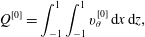 $$\begin{eqnarray}\displaystyle & \displaystyle Q^{[0]}=\int _{-1}^{1}\int _{-1}^{1}v_{\unicode[STIX]{x1D703}}^{[0]}\,\text{d}x\,\text{d}z, & \displaystyle\end{eqnarray}$$
 $$\begin{eqnarray}\displaystyle & \displaystyle Q^{[0]}=2+2\mathop{\sum }_{n=1}^{\infty }\left(\frac{2}{n\unicode[STIX]{x03C0}}\right)^{3}\frac{(-1)^{n}-1}{\unicode[STIX]{x1D6EC}}\tanh \left(\frac{n\unicode[STIX]{x03C0}\unicode[STIX]{x1D6EC}}{2}\right), & \displaystyle\end{eqnarray}$$
 $Q^{[0]}$
stands for flow rate in the planar Couette flow. These solutions can be easily compared to the dimensionless 1D solution (the first term on the right-hand side of (3.14b
)) as
 $Q_{1D}=2$
, in our non-dimensional notation.
3.2.3 Perturbation method
As already discussed, a perturbation method is used to linearize the quasi-linear Oldroyd-B model. The perturbation parameter is considered to be the curvature ratio (
 $\unicode[STIX]{x1D6FF}$
). The series forms of the parameters up to the first order of expansion are
 $$\begin{eqnarray}\displaystyle & \displaystyle \unicode[STIX]{x1D713}=\unicode[STIX]{x1D6FF}\unicode[STIX]{x1D713}^{[1]}, & \displaystyle\end{eqnarray}$$
 $$\begin{eqnarray}\displaystyle & \displaystyle v_{\unicode[STIX]{x1D703}}=v_{\unicode[STIX]{x1D703}}^{[0]}+\unicode[STIX]{x1D6FF}v_{\unicode[STIX]{x1D703}}^{[1]}, & \displaystyle\end{eqnarray}$$
 $$\begin{eqnarray}\displaystyle & \displaystyle P=P^{[0]}+\unicode[STIX]{x1D6FF}P^{[1]}, & \displaystyle\end{eqnarray}$$
 $$\begin{eqnarray}\displaystyle & \displaystyle \unicode[STIX]{x1D70F}=\unicode[STIX]{x1D70F}^{[0]}+\unicode[STIX]{x1D6FF}\unicode[STIX]{x1D70F}^{[1]}. & \displaystyle\end{eqnarray}$$
Here,
 $\unicode[STIX]{x1D713}$
is the secondary flow streamfunction, which is related to the lateral components of the velocity vector via
 $$\begin{eqnarray}\displaystyle & \displaystyle v_{r}=\frac{1}{\unicode[STIX]{x1D6EC}}\frac{\unicode[STIX]{x2202}\unicode[STIX]{x1D713}}{\unicode[STIX]{x2202}z}, & \displaystyle\end{eqnarray}$$
 $$\begin{eqnarray}\displaystyle & \displaystyle v_{z}=-\frac{\unicode[STIX]{x2202}\unicode[STIX]{x1D713}}{\unicode[STIX]{x2202}x}. & \displaystyle\end{eqnarray}$$
In the case that the curvature ratio goes to zero (
 $\unicode[STIX]{x1D6FF}\rightarrow 0$
), one should note that the effect of curvature will be eliminated, so the flow will be rectilinear (i.e. no secondary flow). So, in these cases,
 $\unicode[STIX]{x1D713}$
will be zero and consequently the series form of the streamfunction in (3.15) must have only the first-order term.
3.2.4 Perturbation solution
Substituting the perturbed forms of flow parameters (3.15)–(3.18) into the momentum equations (3.2a
)–(3.2c
) and collecting all the coefficients of order
 $\unicode[STIX]{x1D6FF}^{0}$
, the resulting expression is the same as (3.3). Therefore, the solution to the planar Couette flow (3.13) is the zeroth-order solution of the perturbation method as well. Formally speaking, due to the singularity of both the stress and the shear rate at the corner, this perturbation approach may not be strictly valid in this location near the moving and stationary walls (Hinch Reference Hinch1993). Despite this limitation, we continue with this approach to derive what we will term as an ‘approximate’ analytical solution for the problem. In order to confirm the reasonableness of this approach, we will compare the linearized analytical solution with full nonlinear numerical simulations.
To calculate the solution of the secondary flow up to the first order of perturbation expansion, the same method is employed as was used in the zeroth-order solution. After collecting the terms with the coefficient of order
 $\unicode[STIX]{x1D6FF}^{1}$
, the resulting coefficient expression is (more detailed information about the necessary perturbation steps are presented in appendix A)
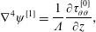 $$\begin{eqnarray}\unicode[STIX]{x1D6FB}^{4}\unicode[STIX]{x1D713}^{[1]}=\frac{1}{\unicode[STIX]{x1D6EC}}\frac{\unicode[STIX]{x2202}\unicode[STIX]{x1D70F}_{\unicode[STIX]{x1D703}\unicode[STIX]{x1D703}}^{[0]}}{\unicode[STIX]{x2202}z},\end{eqnarray}$$
where the biharmonic operator
 $\unicode[STIX]{x1D6FB}^{4}$
is defined as
 $\unicode[STIX]{x1D6FB}^{4}=\unicode[STIX]{x2202}^{4}/\unicode[STIX]{x2202}x^{4}+(2/\unicode[STIX]{x1D6EC}^{2})(\unicode[STIX]{x2202}^{4}/\unicode[STIX]{x2202}z^{2}\unicode[STIX]{x2202}x^{2})+(1/\unicode[STIX]{x1D6EC}^{4})(\unicode[STIX]{x2202}^{4}/\unicode[STIX]{x2202}z^{4})$
. In the case of Newtonian fluids in the creeping-flow limit,
 $\unicode[STIX]{x1D70F}_{\unicode[STIX]{x1D703}\unicode[STIX]{x1D703}}^{[0]}$
is identically zero, as there is no normal stress in fully developed planar Couette flow and the right-hand side of (3.20) is identically zero. So, (3.20) will be a homogenous equation and therefore the general solution to a homogenous equation with homogenous boundary condition is zero (Myint-U & Debnath Reference Myint-U and Debnath2007) (i.e. there must be no secondary flow for Newtonian fluids in the inertialess limit). This reasoning illustrates that, in creeping TC flow, the secondary flow arises due to the existence of non-zero gradients of the first normal-stress difference in viscoelastic fluids (more precisely from the
 $\unicode[STIX]{x1D70F}_{\unicode[STIX]{x1D703}\unicode[STIX]{x1D703}}/r$
term in (3.2a
)). Solution to the non-homogenous linear equation (3.20) can be obtained using standard mathematical approaches (Winters Reference Winters1987; Robertson & Muller Reference Robertson and Muller1996; Jitchote & Robertson Reference Jitchote and Robertson2000; Myint-U & Debnath Reference Myint-U and Debnath2007) subject to zero boundary conditions for velocity in the
 $r$
and
 $z$
directions (due to the large size of these equations, they are not presented here).
4 Numerical model
To check the accuracy and the range of validity of the approximate analytical solution, full nonlinear simulations are carried out using a finite-volume methodology. OpenFOAM software has been utilized to discretize and solve the governing equations (Pimenta & Alves Reference Pimenta and Alves2017). The equations solved are conservation of mass, assuming incompressibility, and momentum:
 $$\begin{eqnarray}\displaystyle & \displaystyle \unicode[STIX]{x1D735}\boldsymbol{\cdot }\boldsymbol{U}=0, & \displaystyle\end{eqnarray}$$
 $$\begin{eqnarray}\displaystyle & \displaystyle Re\left(\frac{\unicode[STIX]{x2202}\boldsymbol{U}}{\unicode[STIX]{x2202}t}+\boldsymbol{U}\boldsymbol{\cdot }\unicode[STIX]{x1D735}\boldsymbol{U}\right)=-\unicode[STIX]{x1D735}P+\unicode[STIX]{x1D6FD}\unicode[STIX]{x1D6FB}^{2}\boldsymbol{U}+\unicode[STIX]{x1D735}\boldsymbol{\cdot }\unicode[STIX]{x1D749}_{p}, & \displaystyle\end{eqnarray}$$
where
 $Re$
is the Reynolds number (i.e.
 $Re=(\tilde{\unicode[STIX]{x1D70C}}\tilde{R}_{i}\tilde{\unicode[STIX]{x1D714}}\tilde{a})/\tilde{\unicode[STIX]{x1D702}}$
, and
 $\tilde{\unicode[STIX]{x1D70C}}$
is the density of the fluid). Here, components of the stress tensor are calculated using a so-called log-conformation approach for the Oldroyd-B constitutive equation (Fattal & Kupferman Reference Fattal and Kupferman2004; Afonso, Pinho & Alves Reference Afonso, Pinho and Alves2012; Pimenta & Alves Reference Pimenta and Alves2017) (already provided in its more standard form relating stress and rate-of-deformation tensors in (2.5) and (2.6)). In order to approximate inertialess conditions, a value of
 $Re=1\times 10^{-3}$
is selected for the Reynolds number in the simulations. Rheological constitutive equations in the kernel-conformation approach are generally written in the form of the conformation tensor,
 $\unicode[STIX]{x1D63C}$
, which is a variance–covariance, symmetric positive definite (SPD) tensor (Afonso et al.
Reference Afonso, Pinho and Alves2012) and is defined as
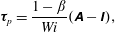 $$\begin{eqnarray}\unicode[STIX]{x1D749}_{p}=\frac{1-\unicode[STIX]{x1D6FD}}{Wi}(\unicode[STIX]{x1D63C}-\unicode[STIX]{x1D644}),\end{eqnarray}$$
where
 $\unicode[STIX]{x1D644}$
is the unit tensor. The conformation tensor is a function of its eigenvectors,
 $\unicode[STIX]{x1D64A}$
, and a diagonal matrix
 $\unicode[STIX]{x1D71E}$
containing its eigenvalues as
 $$\begin{eqnarray}\unicode[STIX]{x1D63C}=\unicode[STIX]{x1D64A}\,\unicode[STIX]{x1D71E}\unicode[STIX]{x1D64A}^{\text{T}},\end{eqnarray}$$
where
 $\unicode[STIX]{x1D64A}$
is an orthogonal matrix that represents the principal axes of the polymeric conformation and
 $\unicode[STIX]{x1D64A}^{\text{T}}$
is the transpose of
 $\unicode[STIX]{x1D64A}$
. Using the natural logarithm as the kernel function,
 $\unicode[STIX]{x1D733}=\unicode[STIX]{x1D64A}\log (\unicode[STIX]{x1D71E})\,\unicode[STIX]{x1D64A}^{\text{T}}$
, the evolution equation for the Oldroyd-B constitutive equation will be represented as
 $$\begin{eqnarray}\frac{\unicode[STIX]{x2202}\unicode[STIX]{x1D733}}{\unicode[STIX]{x2202}t}+\boldsymbol{U}\boldsymbol{\cdot }\unicode[STIX]{x1D735}\unicode[STIX]{x1D733}=\unicode[STIX]{x1D734}\unicode[STIX]{x1D733}-\unicode[STIX]{x1D733}\unicode[STIX]{x1D734}+2\boldsymbol{B}+\frac{1}{Wi}(\text{e}^{-\unicode[STIX]{x1D733}}-\unicode[STIX]{x1D644}),\end{eqnarray}$$
where
 $\unicode[STIX]{x1D734}$
and
 $\boldsymbol{B}$
are antisymmetric pure rotation and symmetric traceless extension components of the velocity gradient, respectively (Fattal & Kupferman Reference Fattal and Kupferman2004; Afonso et al.
Reference Afonso, Pinho and Alves2012) To solve (4.1), (4.2) and (4.5), a Gauss scheme is used to discretize the gradient, divergence and Laplacian terms (Pimenta & Alves Reference Pimenta and Alves2017).
4.1 Geometry and boundary conditions
A schematic of the TC geometry is shown in § 2.1 in figure 1. To probe the effect of aspect ratio (
 $\unicode[STIX]{x1D6EC}=\tilde{b}/\tilde{a}$
) in the creeping flow of viscoelastic fluids in both tall and shallow TC systems, 21 different geometries (
 $\unicode[STIX]{x1D6EC}=0.2$
, 0.3, 0.4, 0.5, 0.6, 0.7, 0.8, 0.9, 1.0, 1.25, 1.5, 1.75, 2.0, 2.5, 3.0, 3.25, 3.5, 3.75, 4.0, 10 and 20) have been modelled.
The implementation of correct boundary conditions at the walls can significantly influence the flow fields and stability criteria in numerical methods. This issue finds notable importance in cases dealing with singularities as we have here in the corner of the moving and stationary walls. The prescribed boundary condition for the stress tensor at walls in OpenFOAM is defined based on 1D shear flow of Newtonian fluids (zero gradient stress at the wall) (Pimenta & Alves Reference Pimenta and Alves2017). Owing to the important role of first normal-stress differences arising from viscoelastic behaviour in the appearance of the secondary flow in the present case, we discovered via initial simulations that implementation of the zero-gradient-stress boundary condition at the wall is not a good choice for our problem. In fact, using this boundary condition we could not obtain converged solutions for any Weissenberg number without ‘regularizing’ the wall velocity, i.e. varying the wall velocity smoothly from 0 to 1 over a finite distance (Sousa et al. Reference Sousa, Poole, Afonso, Pinho, Oliveira, Morozov and Alves2016). In marked contrast, via use of the linear extrapolation approach (Pimenta & Alves Reference Pimenta and Alves2017), we were able to obtain converged solutions without recourse to regularization. In this approach, the stress tensor components at interior faces are obtained by linearly interpolating the cell-centred values, while for the boundary face the value extrapolated in the previous time step is used. This results in an explicit Dirichlet boundary condition, which uses information from the direct neighbours (cells sharing a face) of the cell owning the boundary face (Pimenta & Alves Reference Pimenta and Alves2017).
4.2 Comparison of numerical simulation with analytical solution and effect of mesh
In this section a number of representative data analysing the effect of mesh on the flow distribution are presented to give an overview of numerical accuracy.
Mesh study for the case
 $Wi=0.1,~\unicode[STIX]{x1D6FD}=0.5,~\unicode[STIX]{x1D6FF}=0.1,~\unicode[STIX]{x1D6EC}=1$
.
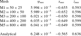
Comparison of the analytical solutions and the numerical simulations is presented in table 1. In this table, five different uniform meshes are shown respectively to study the mesh dependence via the maximum value of the secondary flow (
 $\unicode[STIX]{x1D713}_{max}$
) and its position (
 $x_{max},z_{max}$
). Since the secondary flow is driven by the high shear rate near the corner region between the moving and the stationary walls, to capture this phenomenon better, the mesh should be extremely fine in this region. The presented data suggest that the equivalent of the M3 mesh
 $(200\times 100\unicode[STIX]{x1D6EC})$
is a good choice for simulation. The small difference between the results of the analytical calculations and the numerical simulations can be attributed to the fact that in the corner between the moving wall and the stationary wall a velocity jump exists that causes a singularity in the stress field. Consequently, the chosen perturbation method loses strict validity in this region (Hinch Reference Hinch1993) and we believe this issue is the root cause of the small difference between the approximate analytical solution and the numerical data in terms of the location of the peak streamfunction. Certainly, our mesh-dependence study suggests that the small difference is not simply due to mesh effects in the numerical simulation.
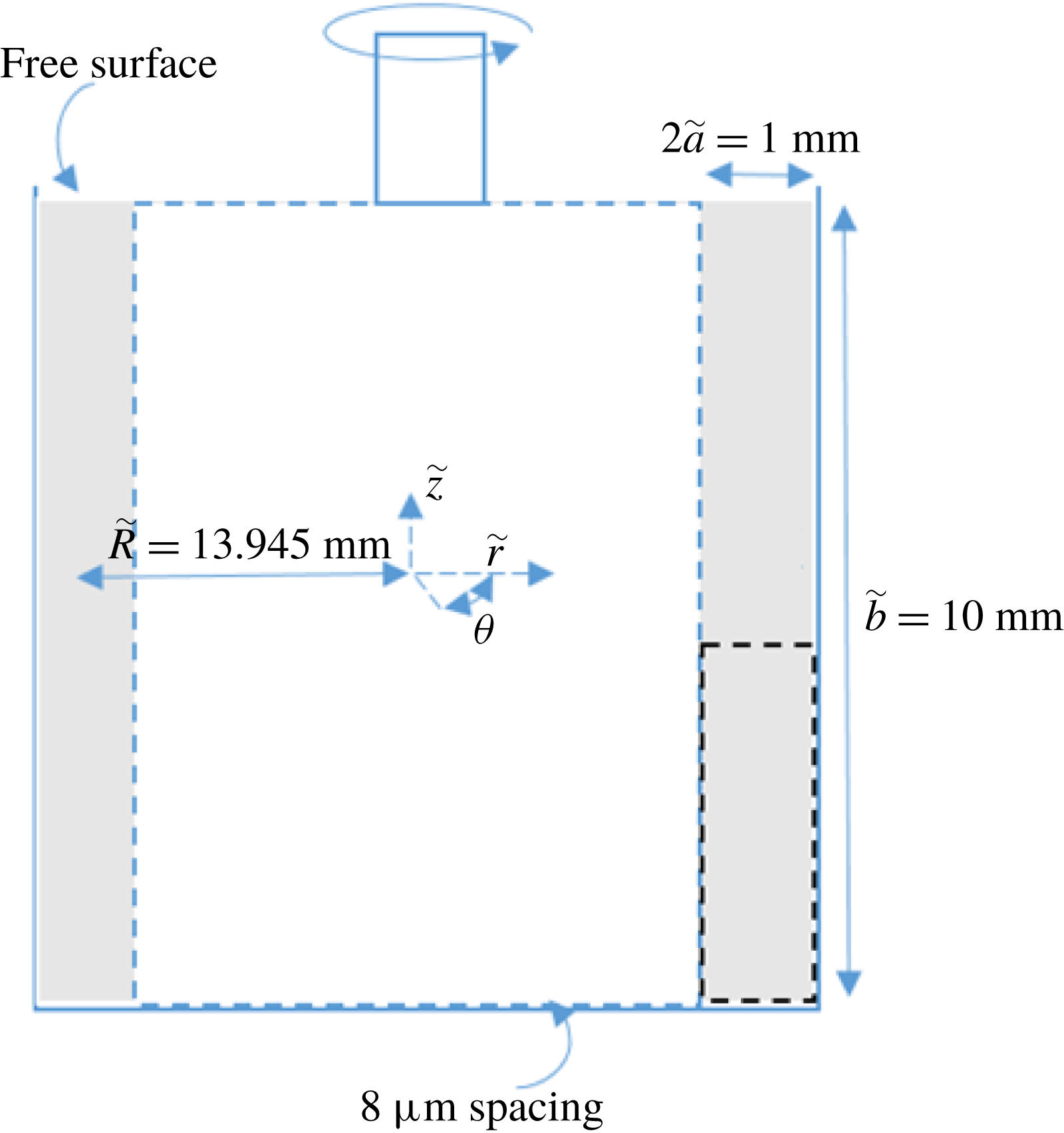
Schematic representation of the TC geometry used for optical visualizations. The dashed rectangle highlights the field of observation of a radial plane illuminated with laser light. Not to scale.
5 Experimental
5.1 Experimental arrangement
The experiments are performed in a transparent TC device fitted to a stress-controlled rheometer (Physica MCR 301) also working in strain-controlled mode via a computer-controlled feedback loop. The TC cell is embedded in a transparent cubical container that ensures temperature control through a water-bath circulation. This configuration of the tank minimizes optical distortions of the images due to refraction caused by the curved interfaces. The rheological properties and the flow behaviour are determined in a Mooney-type TC geometry with inner radius 13.33 mm, gap width 1.13 mm and height 40 mm. For flow visualizations, the geometrical configuration that matches most accurately the problem at hand with the current set-up was investigated and is illustrated in figure 2.
The inner rotating cylinder has a 13.445 mm radius (i.e.
 $\tilde{R}-\tilde{a}$
) and height
 $\tilde{b}=10~\text{mm}$
. In this set-up, due to the stress-free surface, we are essentially investigating just one ‘half’ of the problem described. The gap width is
 $2\tilde{a}=1~\text{mm}$
, which gives an aspect ratio
 $\unicode[STIX]{x1D6EC}=\tilde{b}/\tilde{a}=20$
and curvature ratio
 $\unicode[STIX]{x1D6FF}=\tilde{a}/\tilde{R}=0.04$
. The gap of the TC device is illuminated with a laser sheet propagating along the velocity gradient direction and extending along the vorticity axis. The images of the gap in the velocity gradient/vorticity plane are recorded using a charge-coupled device (CCD) camera equipped with a macro lens.
Two configurations were tested to obtain information regarding the azimuthal structure of the flow. In the first approach, a small amount of sample containing the fluorescent dye is injected along a vertical ‘line’ which is typically 10 mm long (the height of the TC cell) but which also fills the whole gap (1 mm) along the radial direction. This dye is placed slightly upstream from the observation field (typically 1 cm along the azimuthal direction upstream from the observation field) and is illuminated with green laser light (wavelength 532 nm). A supplementary movie available at https://doi.org/10.1017/jfm.2018.746 is included to highlight how such a passive tracer is advected in a Newtonian fluid following a step shear rate to demonstrate our flow visualization technique. In the second approach, flow visualizations are performed by seeding the sample with anisotropic reflective particles (Iriodin, Merck). The structure of the flow is probed by illuminating a cross-section of the gap with red laser light (wavelength 638 nm).
5.2 Working fluids
Aqueous polymer solutions with constant shear viscosity (
 $\tilde{\unicode[STIX]{x1D702}}=239\pm 2~\text{mPa}~\text{s}$
) yet exhibiting elastic properties were prepared by adding 500 ppm (w/w) of a high-molecular-weight polymer (polyethylene oxide (PEO) of
 $M_{w}=4\times 10^{6}~\text{g}~\text{mol}^{-1}$
supplied by Sigma Aldrich) to 42.9 % (w/w) aqueous solvent solution (
 $\tilde{\unicode[STIX]{x1D702}}_{s}=214\pm 2~\text{mPa}~\text{s}$
) of the same polymer with a much lower molecular weight (polyethylene glycol (PEG) of
 $M_{w}=8000~\text{g}~\text{mol}^{-1}$
supplied by Sigma Aldrich). This produces a so-called Boger fluid (Boger Reference Boger1977; James Reference James2009). We estimate the viscosity ratio for this fluid to be 0.89 (i.e.
 $\unicode[STIX]{x1D6FD}=\tilde{\unicode[STIX]{x1D702}}_{s}/\tilde{\unicode[STIX]{x1D702}}=214/239$
). For comparison with the Newtonian case, a glycerine aqueous solution 92% (w/w) is used to match the viscosity
 $(\tilde{\unicode[STIX]{x1D702}}_{N}=240.5\pm 0.7~\text{mPa}~\text{s})$
. For the two samples, the temperature was set to
 $20\pm 0.1\,^{\circ }\text{C}$
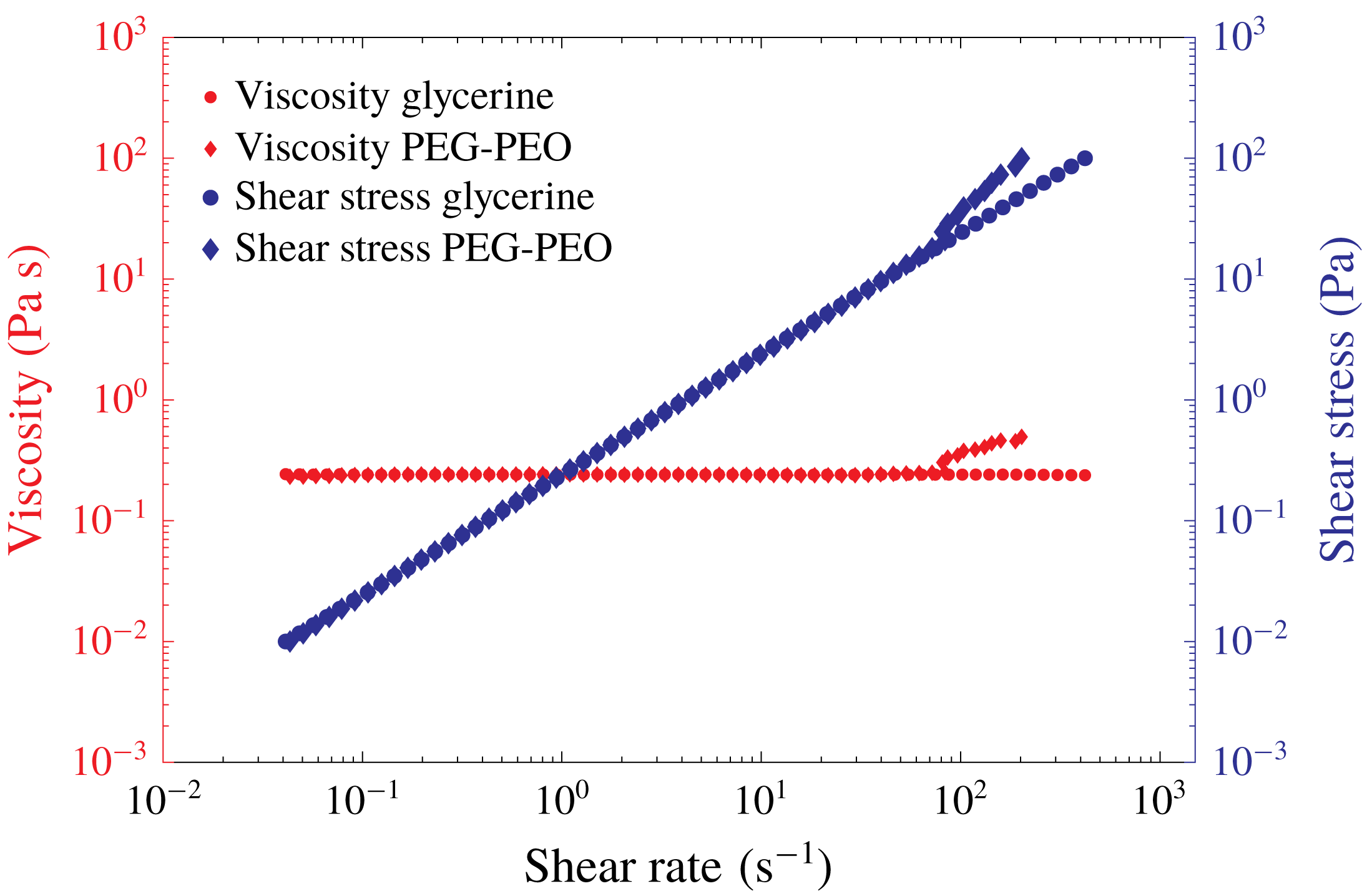
. The variations of the viscosity and shear stress with shear rate for both Newtonian and viscoelastic fluids are presented in figure 3. As can be observed, around a shear rate of
 ${\sim}80~\text{s}^{-1}$
an instability is observed and a deviation between the apparent viscosity of Newtonian and viscoelastic material appears; however, before this critical value, the viscosities of the two fluids are equal and independent of shear rate. To calculate the relaxation time of the polymeric solution, a capillary breakup extensional rheometer (CaBER) (Rodd et al.
Reference Rodd, Scott, Cooper-White and McKinley2004) test is carried out giving a relaxation time of
 $0.27\pm 0.03~\text{s}$
.
Shear stress and shear viscosity as functions of the shear rate for the glycerine solution (●) and for the PEG–PEO solution (♦) at
 $\tilde{T}=20\,^{\circ }\text{C}$
. The data were collected in stress-controlled mode by increasing the shear stress with sampling of 5 s per data point.
6 Results and discussion
In this section a discussion based on a comparison between the analytical, numerical and experimental observations is carried out.
6.1 Planar Couette flow
The flow distribution of the Newtonian creeping-flow finite-aspect-ratio planar Couette flow (zeroth order of the perturbation solution) is shown in figure 4. In order to better understand the effect of aspect ratio, it is useful to define a modified form of aspect ratio as
 $$\begin{eqnarray}\unicode[STIX]{x1D6EC}^{\ast }=\frac{\unicode[STIX]{x1D6EC}}{\unicode[STIX]{x1D6EC}+1}.\end{eqnarray}$$
Using this definition, when the aspect ratio
 $(\unicode[STIX]{x1D6EC})$
changes from zero to infinity, the modified form of the aspect ratio
 $(\unicode[STIX]{x1D6EC}^{\ast })$
varies from zero to one, respectively.
Owing to the absence of curvature and inertia in this case, the flow has a quasi-linear distribution with no secondary flow. According to the rectilinear flow theorem of viscoelastic fluids (Reiner Reference Reiner1945; Rivlin Reference Rivlin1948; Rivlin & Ericksen Reference Rivlin and Ericksen1955; Ericksen Reference Ericksen1956; Green & Rivlin Reference Green and Rivlin1956; Rivlin Reference Rivlin1957), the solution of the velocity profile for viscoelastic fluids with a constant shear viscosity (the Oldroyd-B model in our case) is identical to the Newtonian flow distribution in rectilinear cases. However, it should be noted that the velocity profile for Oldroyd-B fluids generates a normal-stress distribution that consequently influences the pressure distribution, which is different from the Newtonian case.
In figure 4, and all of the other results relating to the contours of the velocity and the streamfunction, the moving wall is the vertical left-hand sidewall. To check the accuracy of the derived zeroth-order solution (
 $\unicode[STIX]{x1D6FF}=0$
), a comparison between numerical simulations and the analytical solution is carried out (as shown in figure 4). In numerical simulations, flow distributions for three different aspect ratios
 $\unicode[STIX]{x1D6EC}^{\ast }\,(\unicode[STIX]{x1D6EC})=0.2\,(0.25)$
, 0.5 (1) and 0.909 (10) with both ANSYS Fluent and OpenFOAM software have been simulated. The geometry consists of three stationary walls and one moving wall. To ensure the flow is fully developed, the non-dimensional length (made dimensionless using
 $a$
) of this domain is chosen to be 1,
 $\unicode[STIX]{x1D6EC}$
and 10 with the number of mesh points 50, 500 and
 $50\times \unicode[STIX]{x1D6EC}$
in the
 $x$
,
 $\unicode[STIX]{x1D703}$
and
 $z$
directions, respectively. As is clear from inspection of figure 4, the numerical simulations exhibit a good agreement with the analytical solution.
Velocity contours for planar Couette flow (‘zeroth-order’ solution, (3.13)) for: (a)
 $\unicode[STIX]{x1D6EC}^{\ast }\,(\unicode[STIX]{x1D6EC})=0.2\,(0.25)$
; (b)
 $\unicode[STIX]{x1D6EC}^{\ast }\,(\unicode[STIX]{x1D6EC})=0.5\,(1)$
; and (c)
 $\unicode[STIX]{x1D6EC}^{\ast }\,(\unicode[STIX]{x1D6EC})=0.909\,(10)$
. Analytical solution (filled contours); full nonlinear solution of Navier–Stokes using finite-volume solver (– – –).
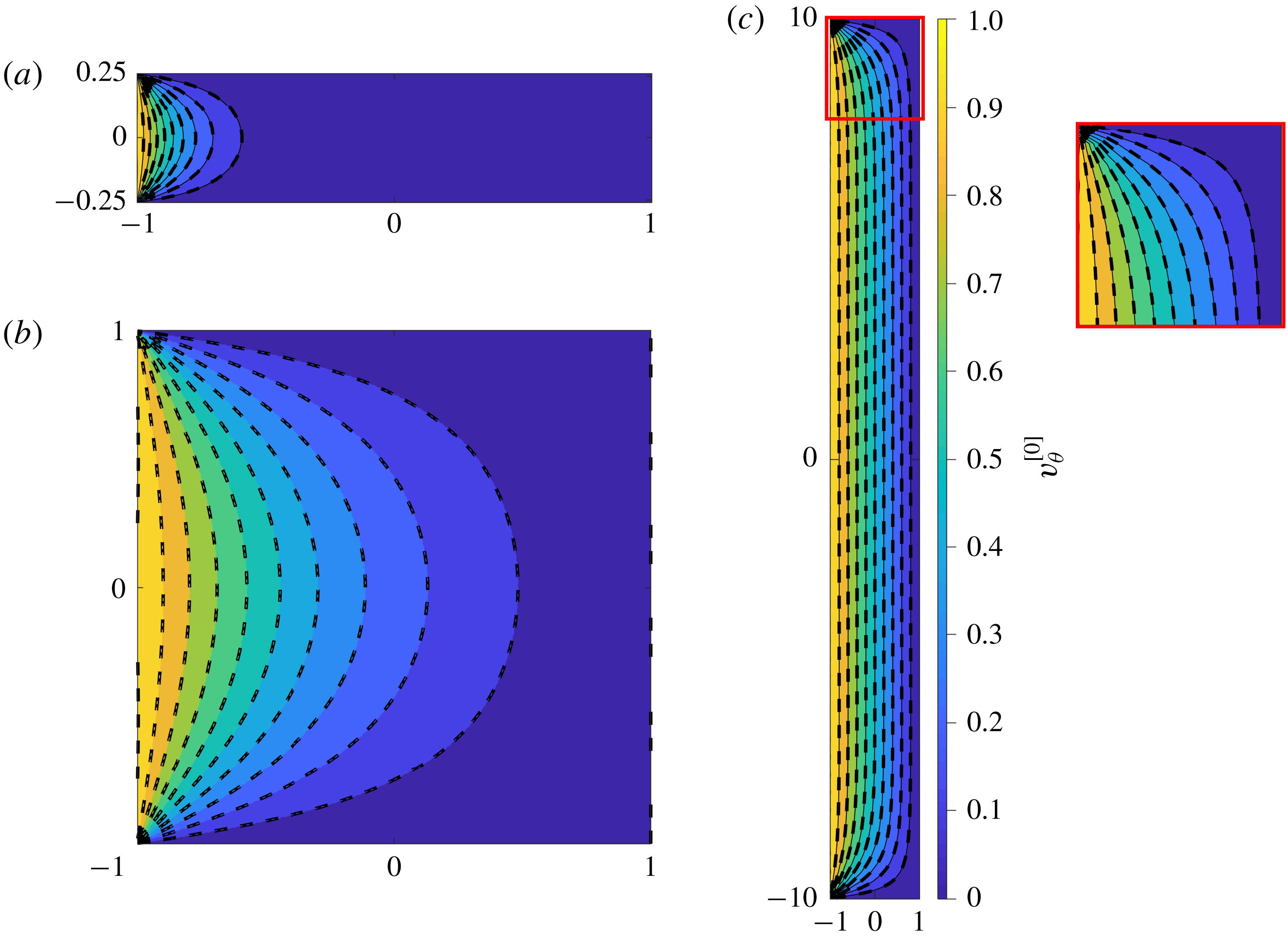
As can be seen, in small aspect ratios, the flow distribution is significantly influenced by the effect of the confining walls (figure 4 a,b) while, when the aspect ratio increases, the effect of the confining walls is limited to the region near the corner between the moving wall and the stationary wall, and the flow distribution in the middle tends towards the 1D linear solution (figure 4 c).
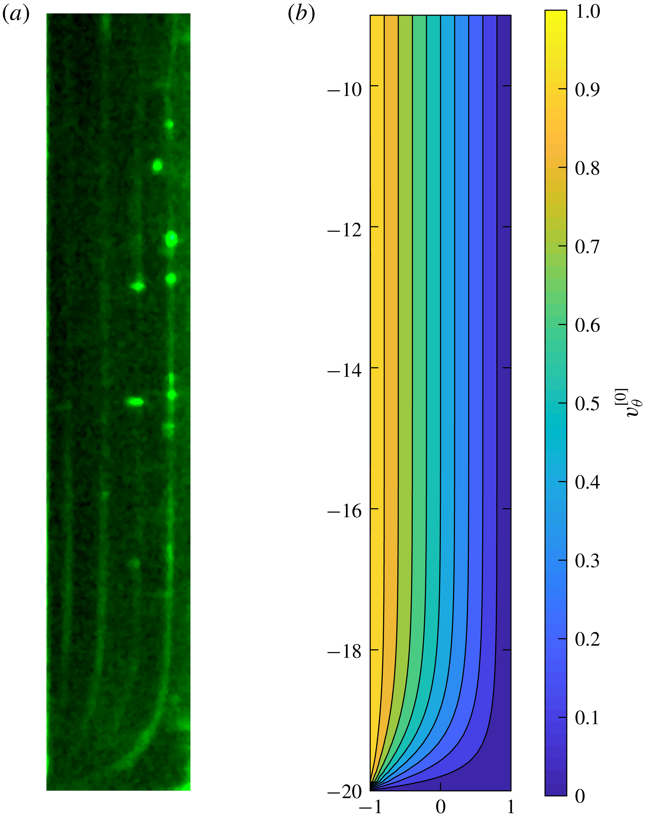
Effect of confining wall for a Newtonian fluid in steady planar Couette flow with aspect ratio
 $\unicode[STIX]{x1D6EC}=\tilde{b}/\tilde{a}=20$
. (a) Snapshot of the lower part of the gap which reflects the advection after five revolutions of a fluorescent dye initially injected at a given location slightly upstream with respect to the observation field. The glycerine solution is sheared at
 $\dot{\tilde{\unicode[STIX]{x1D6FE}}}=30~\text{s}^{-1}$
(
 $Re\sim 5\times 10^{-2}$
). The bright fluorescent dots are due to small bubbles. (b) Creeping-flow axial velocity computed analytically from (3.13).
Experimentally we tested a 92% (w/w) Newtonian glycerine/water solution in a geometrical configuration corresponding to
 $\unicode[STIX]{x1D6EC}=\tilde{b}/\tilde{a}=20$
. Figure 5(a) displays a snapshot of the lower part of the gap taken 14 s after shear start-up at
 $\dot{\tilde{\unicode[STIX]{x1D6FE}}}=30~\text{s}^{-1}$
(
 $Re\sim 5\times 10^{-2}$
). The viscous diffusion time being
 ${\sim}4\times 10^{-3}~\text{s}$
, the velocity profile is fully developed. The fluorescent dye, which is initially injected
 ${\sim}1~\text{cm}$
upstream with respect to the observation field, is convected along the azimuthal direction (see supplementary movie 1 for further information). The fluorescent lines in the picture represent lines of iso-velocity visible after approximately five revolutions. They provide information about the structure of the streamlines in the azimuthal direction. Away from the bottom wall, the picture is compatible with the solution of planar Couette flow; while close to the bottom wall, the confining effect is clearly observed.
The analytical solution computed for the same geometrical conditions (
 $\unicode[STIX]{x1D6EC}=\tilde{b}/\tilde{a}=20$
) and
 $Re=0$
is displayed in figure 5(b). The steady velocity distribution is in good qualitative agreement with the experimental observations. For clarity, we reiterate that the creeping flow of a Newtonian fluid is purely azimuthal (
 $\unicode[STIX]{x1D703}$
) with no motion in the lateral directions, i.e. confirming no secondary flow is observed for creeping Newtonian fluid flow.
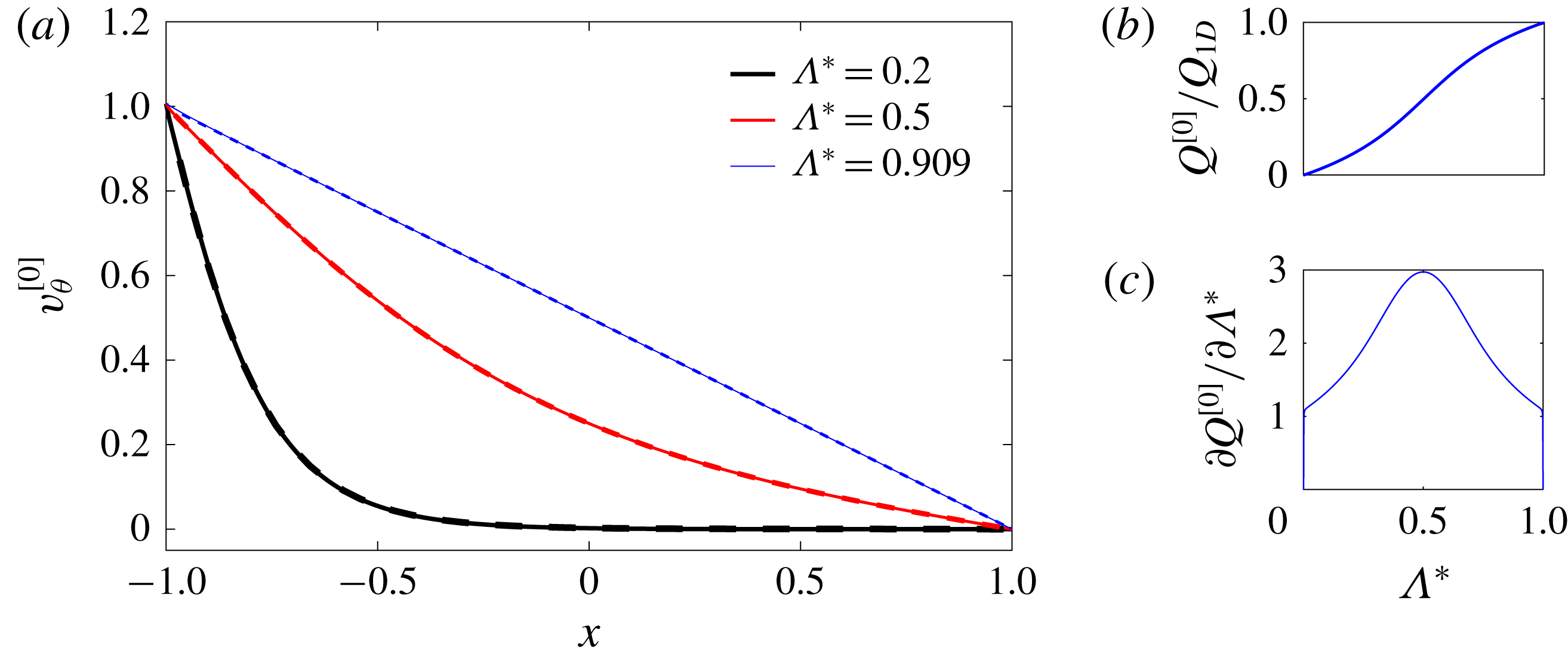
As was previously reported by Taylor (Reference Taylor1923), in the narrow-gap limit, the flow in the TC system for infinite aspect ratio should exhibit a linear distribution along the radial direction. In figure 6(a), the velocity distributions across the gap centreline (i.e. along
 $z=0$
) for different aspect ratios are shown using both analytical and numerical results. The figure shows that the narrow-gap limit is approximately reached by
 $\unicode[STIX]{x1D6EC}^{\ast }=0.909$
(
 $\unicode[STIX]{x1D6EC}=10$
) where the profile is linear, while for smaller normalized aspect ratios
 $\unicode[STIX]{x1D6EC}^{\ast }$
the velocity distribution becomes strongly nonlinear. In figure 6(b,c), the variation of non-dimensional flow rate per unit length, which is normalized with the 1D flow-rate solution (
 $Q^{[0]}/Q_{1D}$
), and its variation with aspect ratio are depicted. In finite-aspect-ratio cases, the flow rate is always smaller than the 1D flow through an equivalent area. This issue is clearly related to the effect of the confining walls resulting in a reduction of the fluid velocity in the region near to the wall. Interestingly, for the unit-aspect-ratio case (
 $\unicode[STIX]{x1D6EC}^{\ast }=0.5$
), the flow rate is reduced to exactly half of the equivalent 1D approximation. Figure 6(c) shows that the effect of normalized aspect ratio is exactly symmetric about
 $\unicode[STIX]{x1D6EC}^{\ast }=0.5$
, highlighting that the asymptotic behaviours as
 $\unicode[STIX]{x1D6EC}^{\ast }\rightarrow 0$
and
 $\unicode[STIX]{x1D6EC}^{\ast }\rightarrow 1$
are equivalent.
(a) Variation of streamwise velocity component across the gap centreline with
 $\unicode[STIX]{x1D6EC}^{\ast }$
: analytical (solid); numerical (dashed). (b) Flow rate for planar Couette normalized by 1D Couette flow rate (linear velocity distribution) versus
 $\unicode[STIX]{x1D6EC}^{\ast }$
. (c) Variation of the flow-rate slope for planar Couette normalized by the 1D Couette flow rate (linear velocity distribution) versus
 $\unicode[STIX]{x1D6EC}^{\ast }$
.
Effect of normalized aspect ratio
 $\unicode[STIX]{x1D6EC}^{\ast }$
on the shear rate normalized with the shear rate of the 1D solution (
 $\dot{\unicode[STIX]{x1D6FE}}_{1D}$
) of planar Couette flow at
 $x=-1$
,
 $z=0$
. Inset:
 $\dot{\unicode[STIX]{x1D6FE}}^{\ast }=f(\unicode[STIX]{x1D6EC}^{\ast })$
in log–log scale.
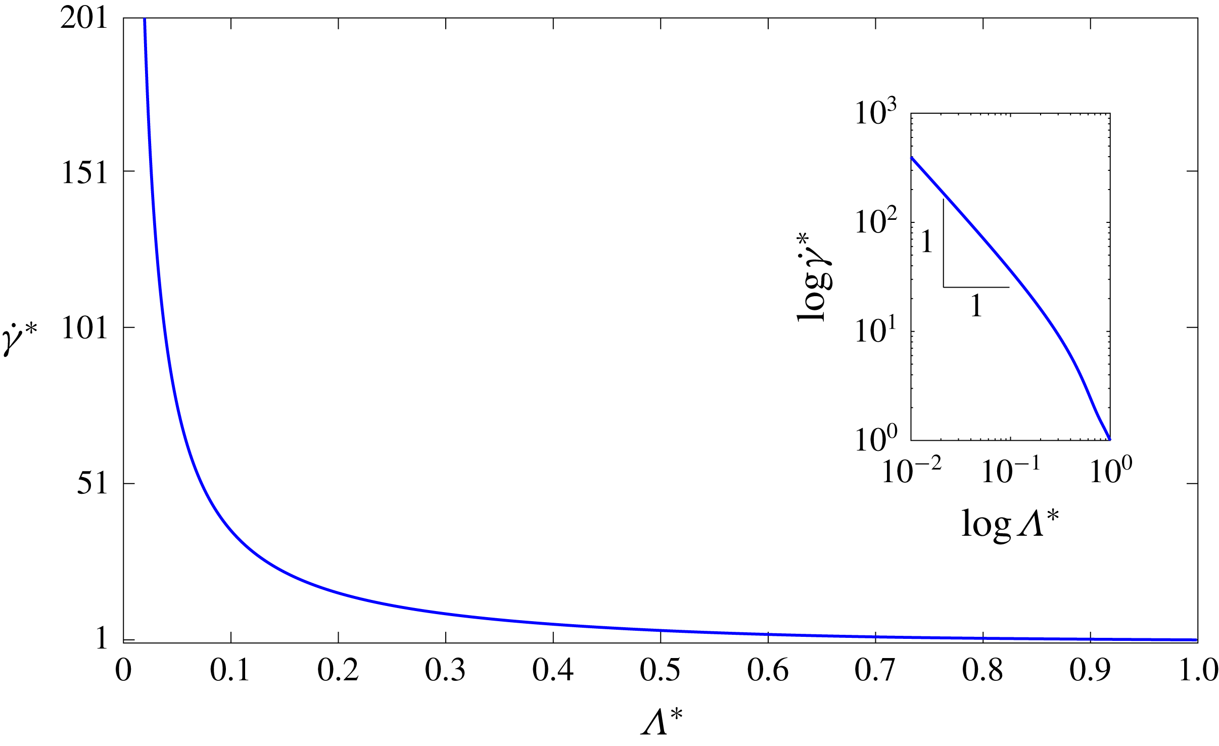
Figure 7 shows that, as the normalized aspect ratio decreases, the ratio of the wall shear rate at the centreline (i.e. at
 $x=-1,~z=0$
) for the two-dimensional (2D) case over the shear rate of the 1D case increases and tends to infinity exhibiting an inverse relationship with the modified aspect ratio (
 $\dot{\unicode[STIX]{x1D6FE}}^{\ast }\sim 1/\unicode[STIX]{x1D6EC}^{\ast }$
) in the limit
 $\unicode[STIX]{x1D6EC}^{\ast }\rightarrow 0$
(see inset in figure 7). The shear rate at higher aspect ratios tends to its 1D solution as can be expected, i.e. as
 $\unicode[STIX]{x1D6EC}^{\ast }\rightarrow 1,~\dot{\unicode[STIX]{x1D6FE}}^{\ast }\rightarrow 1$
. By
 $\unicode[STIX]{x1D6EC}^{\ast }=0.95\,(0.975)$
the shear rate is within 10 % (5 %) of the 1D value.
6.2 Relevance to purely elastic instabilities
Purely elastic instabilities for viscoelastic fluids have received a great deal of attention because of their applications in, for example, mixing and heat transfer (Giesekus Reference Giesekus1966, Reference Giesekus1972; Shaqfeh Reference Shaqfeh1996). A criterion presented by McKinley, Pakdel & Öztekin (Reference McKinley, Pakdel and Öztekin1996) can be used to predict the onset of the purely elastic instability as follows:
 $$\begin{eqnarray}M=\sqrt{\frac{\tilde{\unicode[STIX]{x1D706}}\tilde{U} _{1}}{\tilde{\mathfrak{R}}}\frac{\tilde{\unicode[STIX]{x1D70F}}_{11}}{\tilde{\unicode[STIX]{x1D702}}\dot{\tilde{\unicode[STIX]{x1D6FE}}}}},\end{eqnarray}$$
where
 $\tilde{U} _{1}$
is a velocity scale,
 $\tilde{\mathfrak{R}}$
a local radius of curvature and
 $\tilde{\unicode[STIX]{x1D70F}}_{11}$
is the tensile stress. In this equation, when the
 $M$
parameter reaches a critical value, the instability sets in where the critical magnitude for this parameter (i.e.
 $M_{cr}$
) must be determined from either careful experiments or detailed calculations; e.g. for a 1D TC flow for the Oldroyd-B model with
 $\unicode[STIX]{x1D6FD}=0.5$
using a linear stability analysis, it is determined to be
 $M_{cr}=5.92$
(Larson et al.
Reference Larson, Shaqfeh and Muller1990). In our notation, for the limiting case of Oldroyd-B fluids in shear flows (i.e.
 $\tilde{\unicode[STIX]{x1D70F}}_{11}=2\tilde{\unicode[STIX]{x1D702}}_{p}\tilde{\unicode[STIX]{x1D706}}\dot{\tilde{\unicode[STIX]{x1D6FE}}}^{2}$
assuming
 $\dot{\tilde{\unicode[STIX]{x1D6FE}}}=\tilde{R}_{i}\tilde{\unicode[STIX]{x1D714}}/2\tilde{a}$
for a 1D case) and considering
 $\tilde{U} _{1}=\tilde{R}_{i}\tilde{\unicode[STIX]{x1D714}}$
and
 $\tilde{\mathfrak{R}}=\tilde{R}$
, this criterion can be estimated as (McKinley et al.
Reference McKinley, Pakdel and Öztekin1996)
 $$\begin{eqnarray}M=\sqrt{\unicode[STIX]{x1D6FF}(1-\unicode[STIX]{x1D6FD})}Wi.\end{eqnarray}$$
As shown in figures 6 and 7, the shear rate along the centreline can be significantly influenced by the effect of the confining walls. So, from (6.3), one can expect that the aspect ratio will play an important role in triggering the critical condition where the instability starts. However, as the shear rate is singular at the corner,
 $M$
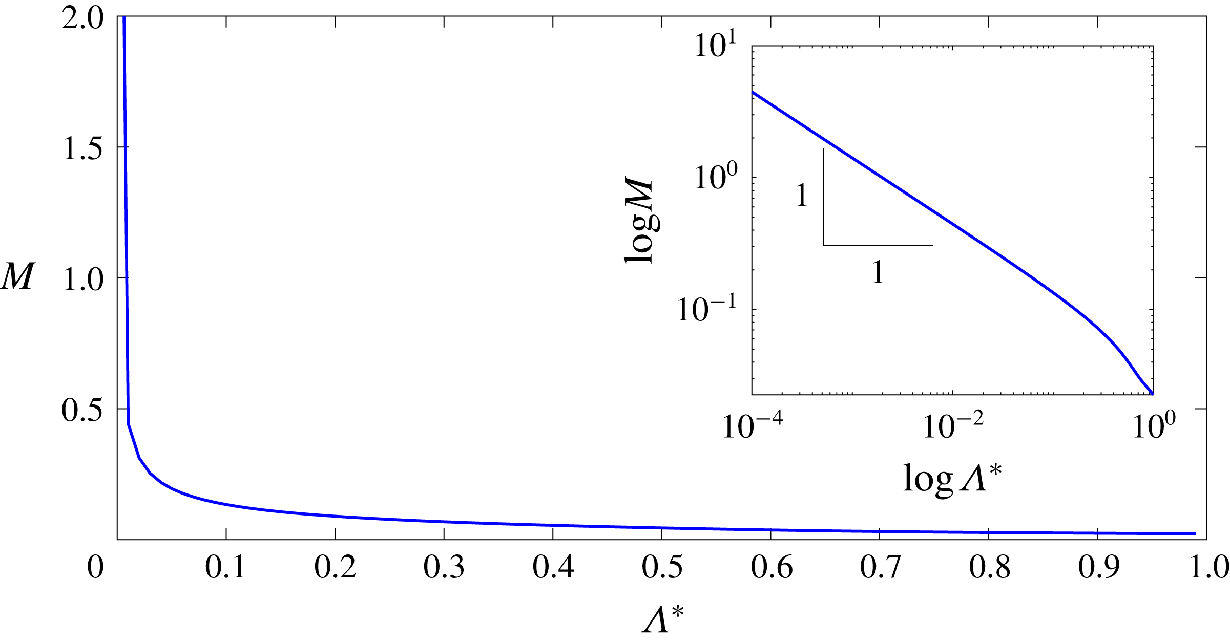
is also singular here based on our analysis. Thus we restrict our analysis here to just centreline conditions. In figure 8 the effect of the modified aspect ratio on the
 $M$
parameter is depicted along the centreline (based on the zeroth-order analytical solution) for a nominal situation of
 $\unicode[STIX]{x1D6FD}=0.5$
,
 $Wi=0.1$
and
 $\unicode[STIX]{x1D6FF}=0.1$
.
Effect of normalized aspect ratio
 $\unicode[STIX]{x1D6EC}^{\ast }$
on the
 $M$
parameter at
 $x=-1$
,
 $z=0$
for the
 $\unicode[STIX]{x1D6FD}=0.5,~Wi=0.1,~\unicode[STIX]{x1D6FF}=0.1$
case.
For this particular case, the
 $M$
parameter for modified aspect ratios of 0.2, 0.5 and 0.8 are calculated as 0.02745, 0.0448 and 0.08941, respectively. Here, setting a constant
 $M_{cr}=5.92$
(i.e. the value calculated from a linear stability analysis in the 1D limit) provides an estimate of the critical values of
 $Wi$
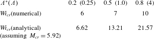
for instability onset, which are 26.56, 21.57, 13.21 and 6.62 for modified aspect ratios of 1 (1D case), 0.8, 0.5 and 0.2, respectively. Once again the centreline values of shear rate are used for this estimate.
Table 2 shows the critical values of
 $Wi$
where the numerical simulation predicts the onset of unsteadiness/instability in comparison to these analytical estimates assuming
 $M_{cr}$
remains the same as the 1D linear stability result (Larson et al.
Reference Larson, Shaqfeh and Muller1990). Our numerical data suggest that
 $M_{cr}$
is not a constant but changes with the aspect ratio. The critical values of
 $M$
where the onset of instability is observed numerically for normalized aspect ratios of 0.2, 0.5 and 0.8 are 1.34, 1.56 and 2.23, respectively. At these values, the numerical results show that the flow becomes time-dependent.
Our analysis would indicate that purely elastic instabilities are more likely to occur at lower Weissenberg numbers for lower-aspect-ratio geometries even when just the centreline shear rates are considered in the analysis. Thus, if one wanted to promote such instabilities, for example to enhance mixing, this could be achieved via small-aspect-ratio geometries. This result may also have important applications for small-angle neutron scattering or flow birefringence studies, which tend to use smaller-aspect-ratio devices.
Critical values of
 $Wi$
for onset of time-dependent flow determined via numerical simulations for case where
 $\unicode[STIX]{x1D6FF}=0.1$
and
 $\unicode[STIX]{x1D6FD}=0.5$
at different aspect ratios.
6.3 Viscoelastic narrow-gap Taylor–Couette flow for arbitrary aspect ratio
As previously discussed with reference to equation (3.20) in § 3.2.4, in the creeping TC flow with finite aspect ratio of viscoelastic fluids, secondary flows are already likely to develop below the purely elastic instability threshold due to the existence of gradients of the first normal-stress difference (from the
 $\unicode[STIX]{x1D70F}_{\unicode[STIX]{x1D703}\unicode[STIX]{x1D703}}/r$
term in (3.2a
)). The combined effect of curvature and the first normal-stress difference results in the movement of the fluid element in the radial direction (as can be seen in (3.2a
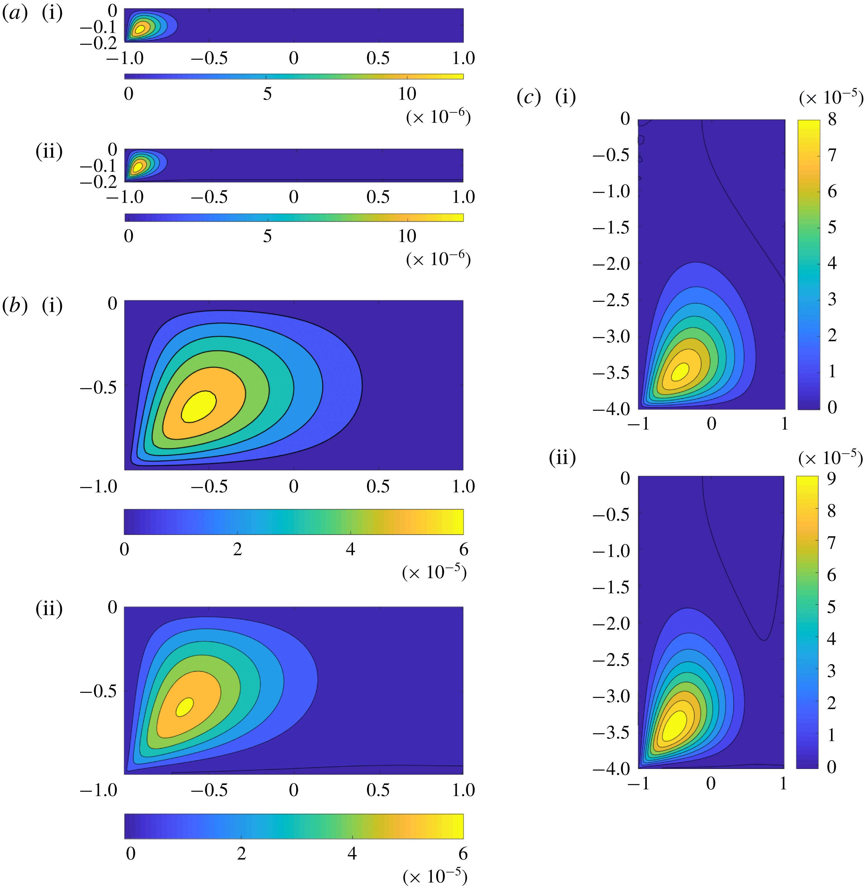
)), but conservation of mass requires the flow to be replaced and, as a result, a pair of secondary flow vortices appears. This mechanism is similar to the one which activates the Dean vortices in creeping viscoelastic flows in curved pipes (Robertson & Muller Reference Robertson and Muller1996; Jitchote & Robertson Reference Jitchote and Robertson2000), but in the current study the flow is driven by wall motion rather than by a pressure gradient. The structure of these secondary flows is presented for three different aspect ratios in figure 9 based on both the analytical solution and numerical simulations. Only the ‘lower’ half of the geometry is depicted in all cases due to the symmetry about
 $z=0$
. The results show that the secondary flows are always located close to the region near the corner of the moving and stationary walls, which is related to the presence of strong gradients in the shear rate and consequently the normal stresses in this region.
Analytical (i) and numerical (ii) estimation of the structure of secondary-flow streamlines for
 $Wi=0.1,~\unicode[STIX]{x1D6FD}=0.5,~\unicode[STIX]{x1D6FF}=0.1$
: (a)
 $\unicode[STIX]{x1D6EC}^{\ast }\,(\unicode[STIX]{x1D6EC})=0.167\,(0.2)$
; (b)
 $\unicode[STIX]{x1D6EC}^{\ast }\,(\unicode[STIX]{x1D6EC})=0.5\,(1.0)$
; (c)
 $\unicode[STIX]{x1D6EC}^{\ast }\,(\unicode[STIX]{x1D6EC})=0.8\,(4.0)$
. Owing to the symmetry about
 $z=0$
, only the lower half of the geometry is depicted.
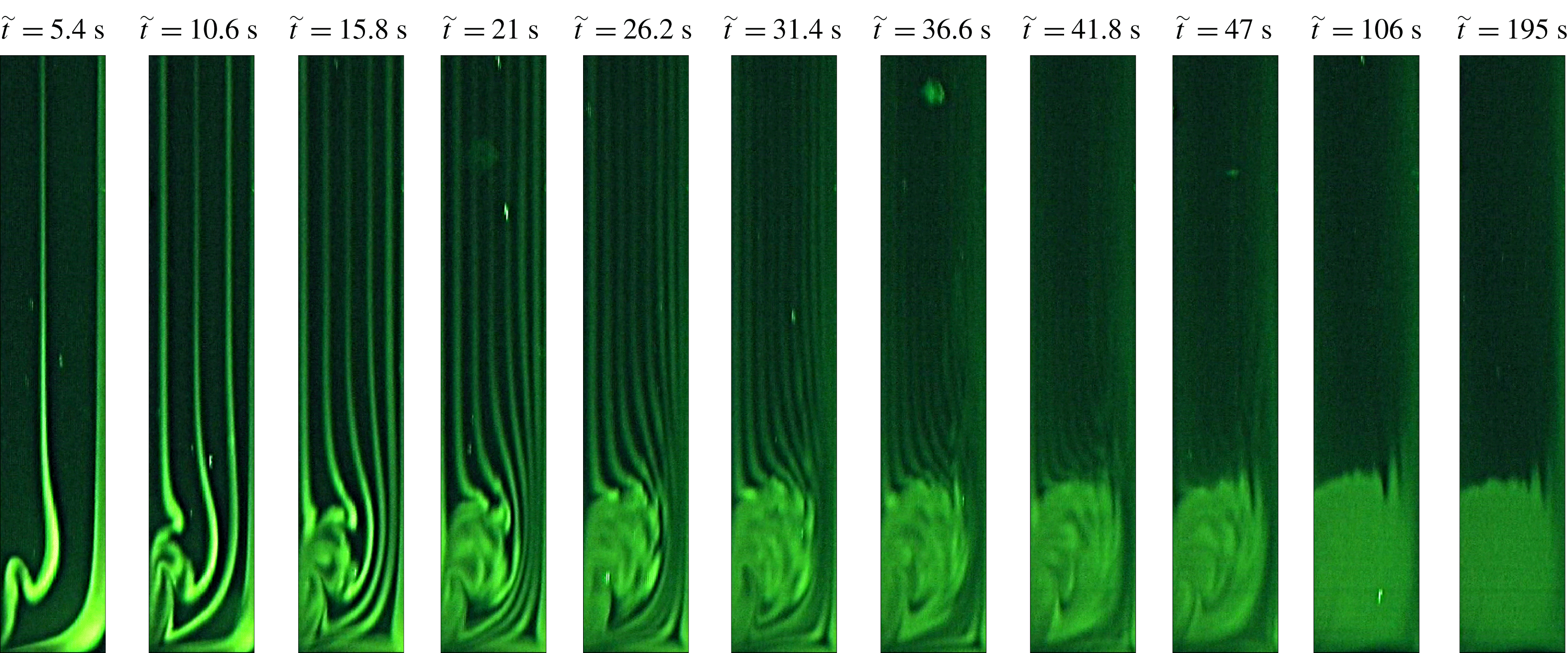
Remarkably, the formation of the secondary flow vortices can be captured experimentally. Figure 10 displays a time sequence of images of the lower part of the gap during shear start-up at
 $\dot{\tilde{\unicode[STIX]{x1D6FE}}}=30~\text{s}^{-1}$
(
 $Re\sim 5\times 10^{-2}$
) (as in the Newtonian case) and
 $Wi\sim 18$
for the 500 ppm (w/w) of PEO in 42.9 % (w/w) aqueous solution of PEG at
 $\tilde{T}=20\,^{\circ }\text{C}$
. Note that the purely elastic instability for this system is triggered for
 $\dot{\tilde{\unicode[STIX]{x1D6FE}}}=80~\text{s}^{-1}$
(see figure 3). Close to the bottom wall, the iso-velocity lines exhibit successive foldings due to the development of a vortex from the corner between the moving wall and the fixed bottom wall. The iso-velocity lines and the structure of the corner vortex can be observed during several tens of seconds before homogenization due to molecular diffusion of the fluorescent dye.
Time sequence of images illustrating the formation of the corner secondary flow structure for a 500 ppm (w/w) of PEO in 42.9 % (w/w) aqueous solution of PEG at
 $\tilde{T}=20\,^{\circ }\text{C}$
. The applied shear rate is
 $\dot{\tilde{\unicode[STIX]{x1D6FE}}}=30~\text{s}^{-1}$
(
 $\unicode[STIX]{x1D6FF}=0.04$
,
 $\unicode[STIX]{x1D6EC}=20$
,
 $Re=5\times 10^{-2}$
,
 $Wi=18$
,
 $\unicode[STIX]{x1D6FD}=0.89$
). The observation field covers 56 % of the height of the cylinders in the
 $z$
direction and the full gap (1 mm) in the radial direction.
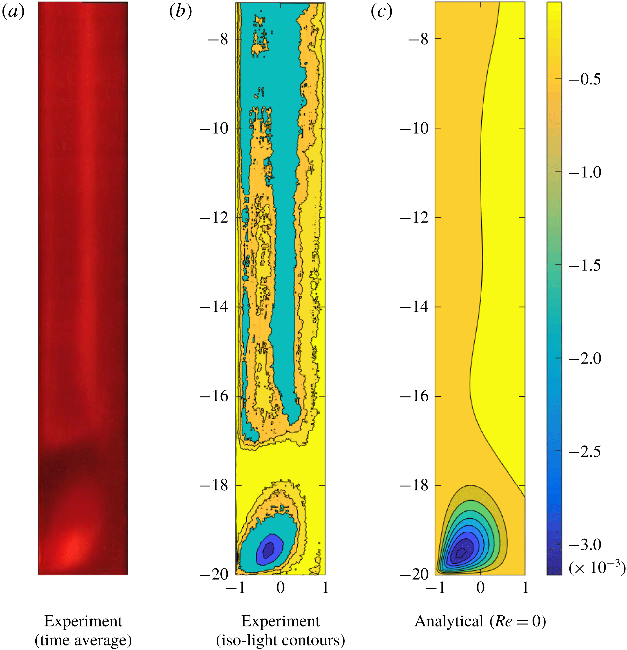
In order to better capture the structure of the corner vortex at long times, flow visualizations were also performed using anisotropic reflective particles seeded in the sample. In this configuration the gap of the TC device is illuminated with red laser light. Figure 11(a) is obtained by taking a moving average over 100 s of sequential images when the steady-state regime is achieved. From this picture, iso-light contours can be extracted (figure 11
b). The position of the eye of the corner secondary flow and its structure show a good qualitative agreement with the result obtained based on the analytical solution for the case
 $\unicode[STIX]{x1D6FF}=0.04,~\unicode[STIX]{x1D6EC}=20,~Re=0,~Wi=18,~\unicode[STIX]{x1D6FD}=0.89$
(figure 11
c). We note that, strictly speaking, the analytical solution is being used outside of its range of validity at this Weissenberg number, and so this comparison is best viewed as purely qualitative in terms of secondary flow structure.
Comparison of the corner secondary flow between the analytical (
 $x_{\unicode[STIX]{x1D713}_{min}}=-0.45,~z_{\unicode[STIX]{x1D713}_{min}}=-19.46$
) and experimental observation (
 $x_{\unicode[STIX]{x1D713}_{min}}=-0.52,~z_{\unicode[STIX]{x1D713}_{min}}=-19.72$
) of 500 ppm (w/w) of PEO in 42.9 % (w/w) aqueous solution of PEG at
 $\tilde{T}=20\,^{\circ }\text{C}$
. The applied shear rate is
 $\dot{\unicode[STIX]{x1D6FE}}=30~\text{s}^{-1}$
. Experiments:
 $\unicode[STIX]{x1D6FF}=0.04,~\unicode[STIX]{x1D6EC}=20,~Re=5\times 10^{-2},~Wi=18,~\unicode[STIX]{x1D6FD}=0.89$
. Analytical:
 $\unicode[STIX]{x1D6FF}=0.04,~\unicode[STIX]{x1D6EC}=20,~Re=0,~Wi=18,~\unicode[STIX]{x1D6FD}=0.89$
.
The location of the eye of maximum vortex (or the centre of the secondary flow) is given in figure 12 based on analytical and numerical results. The location of the maximum vortex starts to move from a region close to the moving wall in the radial direction while its position stays constant in
 $z$
, when the aspect ratio increases from 0.1 to 1. As the aspect ratio increases from 1 to 2, the location of the maximum vortex migrates to a new position in both the radial and
 $z$
directions. Finally, it can be seen that, by further increasing the aspect ratio, the eye of the vortex remains at a constant radial location while it migrates towards the top wall (i.e.
 $z\rightarrow 1$
). Although these trends are the same for both the analytical and numerical results, there is a systematic quantitative variation between the two approaches as had already been observed in § 4.2 where the mesh dependence was discussed for the square aspect-ratio case.
Locations of the eyes of maximum vortices for
 $Wi=0.1,~\unicode[STIX]{x1D6FD}=0.5,~\unicode[STIX]{x1D6FF}=0.1$
in different aspect ratios
 $\unicode[STIX]{x1D6EC}=0.2$
, 0.3, 0.4, 0.5, 0.6, 0.7, 0.8, 0.9, 1.0, 1.25, 1.5, 1.75, 2.0, 2.5, 3.0, 3.5 and 4.0 (diamonds, from left to right, respectively).

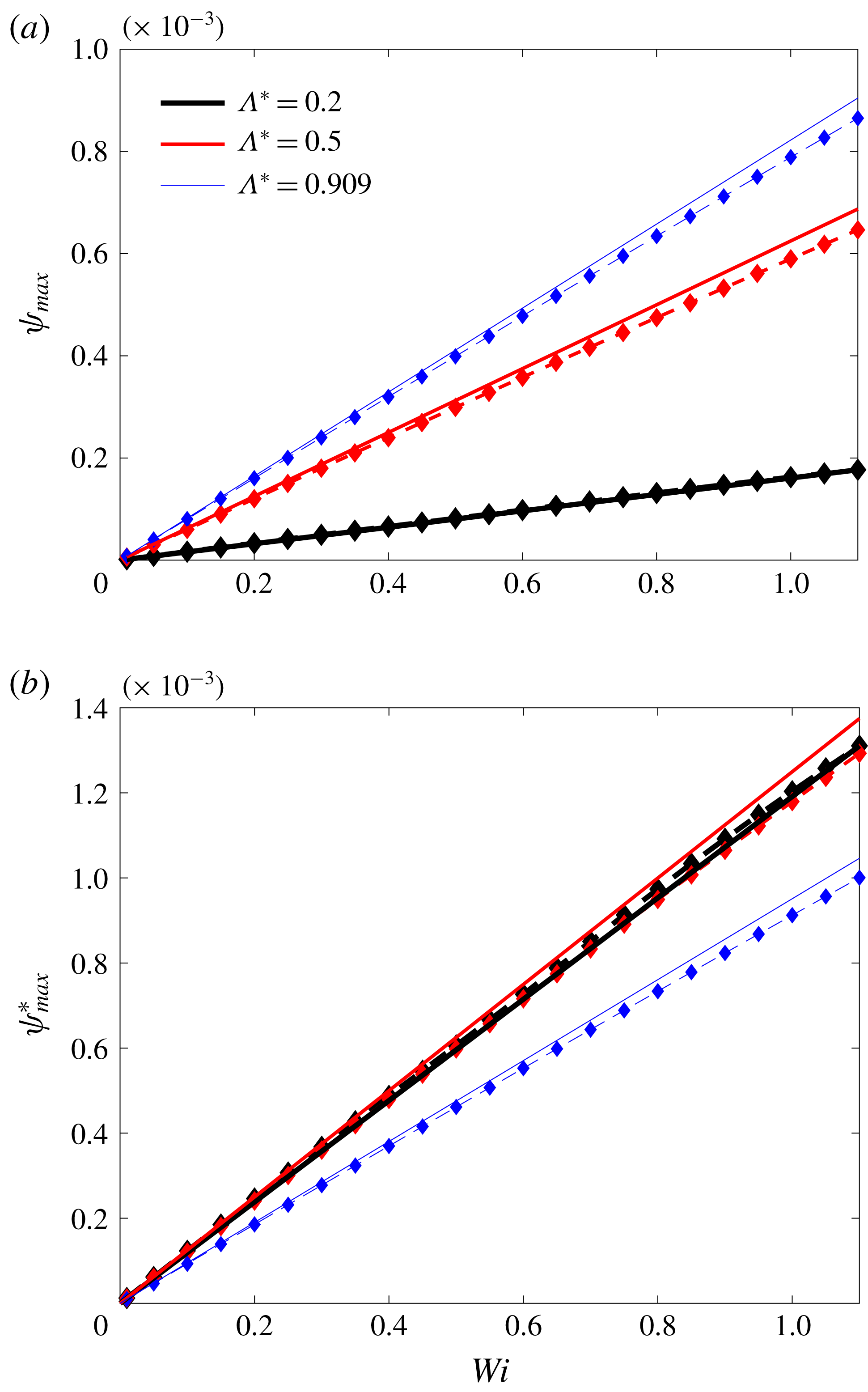
To analyse the range of validity of the perturbation method, the variation of the maximum value of the secondary flow streamfunction with
 $Wi$
for both the analytical and the numerical solutions are presented in figure 13. The data show that this parameter increases linearly with an increase in the Weissenberg number in the range of
 $0<Wi<1.1$
, confirming that the approximate analytical solution data for this range is in an acceptable agreement with the full nonlinear numerical simulation. As shown in figure 6(b), the flow rate decreases with a decrease in the aspect ratio. Figure 13(a) shows that the same trend may also be observed for the maximum value of the secondary flow streamfunction, which may seem, at first glance, reasonable but, as the secondary flow is driven by a gradient induced by the confining walls, this is counter-intuitive, as these effects would be expected to increase as the confining walls become more important (
 $\unicode[STIX]{x1D6EC}\rightarrow 0$
). This confusion can be attributed to the manner in which velocity components and, consequently, the secondary flow streamfunction are made dimensionless. As also shown in figure 6(b), a decrease in the aspect ratio is followed by a decrease in the magnitude of the average velocity throughout the gap. To better discuss the effect of confining walls on the secondary flow, we therefore suggest to use the mean value of the main velocity as the reference velocity in figure 13(b) rather than the wall velocity. In this manner, one can see how the magnitude of the secondary flow streamfunction is scaled with respect to the mean value of the velocity at the same aspect ratio. Using this normalization, it can be shown that, although the magnitude of the main velocity is decreased as the aspect ratio decreases, the ratio of the magnitude of the secondary flow velocity relative to the mean velocity increases, confirming the fact that lateral components of the velocity get stronger as the confining effect of the walls increases (
 $\unicode[STIX]{x1D6EC}\rightarrow 0$
).
Variation of
 $\unicode[STIX]{x1D713}_{max}$
with
 $Wi$
for
 $\unicode[STIX]{x1D6FD}=0.5$
and
 $\unicode[STIX]{x1D6FF}=0.1$
in different aspect ratios of
 $\unicode[STIX]{x1D6EC}^{\ast }\,(\unicode[STIX]{x1D6EC})=0.2\,(0.25)$
,
 $\unicode[STIX]{x1D6EC}^{\ast }\,(\unicode[STIX]{x1D6EC})=0.5\,(1.0)$
, and
 $\unicode[STIX]{x1D6EC}^{\ast }\,(\unicode[STIX]{x1D6EC})=0.909\,(10)$
: (a) normalized with wall velocity and (b) normalized with mean value of main velocity. The solid line shows the analytical solution and the dashed line with diamonds highlights the numerical data.
7 Conclusions
In this work, based on both a linear analytical perturbation approach and full nonlinear numerical simulations using a finite-volume technique, the effect of confining walls on the inertialess, viscoelastic narrow-gap TC system was investigated and compared with experimental observations. The results show that, for any finite aspect ratio, a pair of secondary flow vortices exists for any non-zero elasticity (i.e.
 $Wi>0$
), in excellent qualitative agreement with the experiments. This secondary flow appears due to the presence of gradients of the first normal-stress difference (more precisely from the
 $\unicode[STIX]{x1D70F}_{\unicode[STIX]{x1D703}\unicode[STIX]{x1D703}}/r$
term in (3.2a
)). The confining walls on the top and bottom of the geometry can significantly influence the flow distribution through the gap, and the average velocity in the narrow gap is always smaller than the 1D case.
The confining effect of the walls can modify the threshold of the purely elastic instability which is known to occur in TC systems. Based on our full nonlinear simulations, the
 $M_{cr}$
parameter of McKinley et al. (Reference McKinley, Pakdel and Öztekin1996) is not a constant for the finite-aspect-ratio cases but a weak function of the aspect ratio of the geometry. Nevertheless the values of the
 $M_{cr}$
parameter obtained (1.3–2.2) are broadly consistent with values obtained in purely elastic instabilities for other flows (McKinley et al.
Reference McKinley, Pakdel and Öztekin1996; Pakdel & McKinley Reference Pakdel and McKinley1998; Alves & Poole Reference Alves and Poole2007; Zilz et al.
Reference Zilz, Poole, Alves, Bartolo, Levaché and Lindner2012; Sousa et al.
Reference Sousa, Poole, Afonso, Pinho, Oliveira, Morozov and Alves2016). Our analysis would indicate that purely elastic instabilities are more likely to occur at lower Weissenberg numbers for lower-aspect-ratio geometries and this could be used to promote such instabilities, e.g. to enhance mixing. Our results may also have important applications for TC devices used in small-angle neutron scattering or flow birefringence experiments, which tend to use smaller aspect ratios.
Acknowledgements
The authors would like to express their gratitude to Professor G. McKinley (MIT, USA) for a series of valuable suggestions. S.L. acknowledges funding from the Institut Universitaire de France. R.J.P. gratefully acknowledges funding from the EPSRC (UK) through grant no. EP/M025187/1. Finally, we would like to sincerely thank one of the anonymous referees for suggesting the use of a polar cylindrical coordinate system and their independent derivation of the base-flow solution.
Supplementary movie
A supplementary movie is available at https://doi.org/10.1017/jfm.2018.746.
Appendix A
Owing to the quasi-linear form of the Oldroyd-B constitutive equation, a perturbation method is implemented. The perturbed form of the stress and deformation tensor up to the first order of expansion may be presented as
 $$\begin{eqnarray}\displaystyle & \displaystyle \unicode[STIX]{x1D749}=\unicode[STIX]{x1D749}^{[0]}+\unicode[STIX]{x1D6FF}^{1}\unicode[STIX]{x1D749}^{[1]}, & \displaystyle\end{eqnarray}$$
 $$\begin{eqnarray}\displaystyle & \displaystyle \unicode[STIX]{x1D63F}=\unicode[STIX]{x1D63F}^{[0]}+\unicode[STIX]{x1D6FF}^{1}\unicode[STIX]{x1D63F}^{[1]}. & \displaystyle\end{eqnarray}$$
After substituting (A 1) and (A 2) into the polymeric part of the Oldroyd-B constitutive equation, the linearized form of the zeroth order of the stress tensor for the chosen polar cylindrical coordinate system can be obtained. In the absence of curvature,
 $u_{0}$
and
 $w_{0}$
are equal to zero (i.e. no secondary flow in the straight Couette flow) and the zeroth-order stress tensor for the polymeric contribution of the Oldroyd-B constitutive equation can be obtained as follows:
 $$\begin{eqnarray}\displaystyle & \displaystyle \unicode[STIX]{x1D70F}_{p,rz}^{[0]}=\unicode[STIX]{x1D70F}_{p,rr}^{[0]}=\unicode[STIX]{x1D70F}_{p,zz}^{[0]}=0, & \displaystyle\end{eqnarray}$$
 $$\begin{eqnarray}\displaystyle & \displaystyle \unicode[STIX]{x1D70F}_{p,\unicode[STIX]{x1D703}\unicode[STIX]{x1D703}}^{[0]}=2Wi(1-\unicode[STIX]{x1D6FD})\left[\left(\frac{\unicode[STIX]{x2202}v_{\unicode[STIX]{x1D703}}^{[0]}}{\unicode[STIX]{x2202}x}\right)^{2}+\frac{1}{\unicode[STIX]{x1D6EC}^{2}}\left(\frac{\unicode[STIX]{x2202}v_{\unicode[STIX]{x1D703}}^{[0]}}{\unicode[STIX]{x2202}z}\right)^{2}\right], & \displaystyle\end{eqnarray}$$
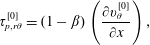 $$\begin{eqnarray}\displaystyle & \displaystyle \unicode[STIX]{x1D70F}_{p,r\unicode[STIX]{x1D703}}^{[0]}=(1-\unicode[STIX]{x1D6FD})\left(\frac{\unicode[STIX]{x2202}v_{\unicode[STIX]{x1D703}}^{[0]}}{\unicode[STIX]{x2202}x}\right), & \displaystyle\end{eqnarray}$$
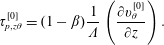 $$\begin{eqnarray}\displaystyle & \displaystyle \unicode[STIX]{x1D70F}_{p,z\unicode[STIX]{x1D703}}^{[0]}=(1-\unicode[STIX]{x1D6FD})\frac{1}{\unicode[STIX]{x1D6EC}}\left(\frac{\unicode[STIX]{x2202}v_{\unicode[STIX]{x1D703}}^{[0]}}{\unicode[STIX]{x2202}z}\right). & \displaystyle\end{eqnarray}$$
Using the same approach and collecting the effective terms in the calculation up to first order of the streamfunction, the corresponding stress components related to the polymeric contribution of the Oldroyd-B constitutive equation may be calculated as follows:
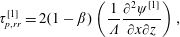 $$\begin{eqnarray}\displaystyle & \displaystyle \unicode[STIX]{x1D70F}_{p,rr}^{[1]}=2(1-\unicode[STIX]{x1D6FD})\left(\frac{1}{\unicode[STIX]{x1D6EC}}\frac{\unicode[STIX]{x2202}^{2}\unicode[STIX]{x1D713}^{[1]}}{\unicode[STIX]{x2202}x\unicode[STIX]{x2202}z}\right), & \displaystyle\end{eqnarray}$$
 $$\begin{eqnarray}\displaystyle & \displaystyle \unicode[STIX]{x1D70F}_{p,rz}^{[1]}=(1-\unicode[STIX]{x1D6FD})\left(\frac{1}{\unicode[STIX]{x1D6EC}^{2}}\frac{\unicode[STIX]{x2202}^{2}\unicode[STIX]{x1D713}^{[1]}}{\unicode[STIX]{x2202}z^{2}}-\frac{\unicode[STIX]{x2202}^{2}\unicode[STIX]{x1D713}^{[1]}}{\unicode[STIX]{x2202}x^{2}}\right), & \displaystyle\end{eqnarray}$$
 $$\begin{eqnarray}\displaystyle & \displaystyle \unicode[STIX]{x1D70F}_{p,zz}^{[1]}=-2(1-\unicode[STIX]{x1D6FD})\left(\frac{1}{\unicode[STIX]{x1D6EC}}\frac{\unicode[STIX]{x2202}^{2}\unicode[STIX]{x1D713}^{[1]}}{\unicode[STIX]{x2202}x\unicode[STIX]{x2202}z}\right). & \displaystyle\end{eqnarray}$$


 Open access

