Endogenous Formation of Free Trade Agreements: Evidence from the Zollverein's Impact on Market Integration

Wolfgang Keller; Carol H. Shiue

doi:10.1017/S0022050714000898

Endogenous Formation of Free Trade Agreements: Evidence from the Zollverein's Impact on Market Integration

Published online by Cambridge University Press: 27 November 2014

Wolfgang Keller and

Carol H. Shiue

Show author details

Wolfgang Keller: Affiliation:
Professor, Department of Economics, University of Colorado, Boulder, CO, 80309, NBER, CESifo, and CEPR.. E-mail: wolfgang.keller@colorado.edu.
Carol H. Shiue: Affiliation:
Associate Professor, Department of Economics, University of Colorado, Boulder, CO, 80309, NBER, CESifo, and CEPR..

Article contents

Abstract
Germany's Nineteenth Century Trade: The Zollverein Treaties
DATA
EMPIRICAL RESULTS
REDUCED-FORM RESULTS
CONCLUDING DISCUSSION
Footnotes
References

Rights & Permissions

Abstract

The Zollverein was arguably the most important free trade agreement of the nineteenth century. Although 1834 is the official date of the Zollverein's establishment, member states joined in a non-random sequence over several decades because the benefits of becoming a member increased, both as the size of the union increased, and as membership in the union became increasingly important for accessing foreign markets. We incorporate the endogenous effects of accession into an estimate of the economic impact of the Zollverein customs union. Our estimated effects are several times larger than simple estimates that do not take these effects into account.

Information

Type: Articles
Information: The Journal of Economic History , Volume 74 , Issue 4 , December 2014, pp. 1168 - 1204
DOI: https://doi.org/10.1017/S0022050714000898 [Opens in a new window]
Copyright: Copyright © The Economic History Association 2014

The German Zollverein of 1834 was arguably the most important regional free trade agreement of the nineteenth century. It was the first time that politically independent states removed trade barriers between themselves and delegated tariff-setting authority to a higher body. Although other treaties can be found, none were as encompassing or long-lived. Jacob Viner (Reference Viner1950, p. 97) called it the “classic example” of a customs union. The importance of the Zollverein was magnified by the fact that prior to union, German states had long been divided into an extraordinary number of small economic zones that implemented their own tariff collections at the borders. Clearly, this state of affairs made things difficult for traders. Although the plethora of polities shrank during the Napoleonic wars, before the treaty was signed in 1834, some300 different administrative political borders remained among German states.Footnote ¹

The economist Friedrich List, head of the Union of Merchants (der Deutsche Handels- and Gewerbeverein), described in colorful terms the scale of the problem in a petition to the German parliament in 1819:

The numerous customs barriers “cripple internal trade and produce the same effect as ligatures which prevent the free circulation of blood. The merchants trading between Hamburg and Austria, or Berlin and Switzerland must traverse ten states, must learn ten customs tariffs, must pay ten successive transit dues. Anyone who is unfortunate enough as to live on the boundary line between three or four states spends his days among hostile tax-gatherers and customs house officials. He is a man without country.”Footnote ²

The Zollverein abolished tariff barriers among member states, and all members agreed to a single external tariff. Over time, the reduction of trade barriers may have also enhanced growth and development in the region (Henderson Reference Henderson1959; Bairoch Reference Bairoch, Mathias and Pollard1989). Given the importance of the Zollverein to the history of trade agreements, it is surprising that we still know little about its actual trade impact. While there are studies on overall trends in Europe towards deregulation and others on the impact of trade reform of the nineteenth century in France, Sweden, and Italy (Federico and Tena Reference Federico and Tena1998; Persson Reference Persson1999), the Zollverein is not yet well understood. Its importance in historical accounts, thus, is overshadowed by the lack of empirical tests of the claims that the Zollverein had significant economic consequences for trade. This paper aims to fill the gap.

We study the Zollverein's effect on trade by examining the convergence of wheat prices across 40 cities located in 14 different German states.Footnote ³ The year 1834 is the official date of the beginning of the German Zollverein since after this date, states gradually started to join the union. A simple approach to examine the impact of trade policies would be to compare the fall in price differentials exhibited by Zollverein versus non-Zollverein-states after a point in time, namely the year 1834. This approach, however, would be flawed for the reason that states that joined the customs union early on were likely to be different from states that would join later, and the differences could systematically change the amount of price convergence.Footnote ⁴ Moreover, if establishing the customs union was either assisted or motivated by the fact that price gaps were falling anyway in the nineteenth century for other reasons, then reverse causation could be a concern.

As we show these concerns are important. First, failure to take them into account results in a downward bias of the impact of the Zollverein on price convergence. Second, the systematic differences between early joiners and late joiners also provide the key for our correction of the biased regression estimates. We take advantage of the historical setting in nineteenth century Germany by using market access variables to predict individual states’ propensity to join the Zollverein. As the membership of the Zollverein under the leadership of Prussia increased in numbers, some German states feared that remaining outside the Zollverein would severely reduce their access to the Northern German sea coast and the gains to international trade available from that location (Keller and Shiue Reference Keller and Shiue2008; Ploeckl Reference Ploeckl2010a).Footnote ⁵ Moreover, the external border of the Zollverein imposed higher costs on the states in Germany's south than those in its north, because the latter did not have to cross the Zollverein customs border to trade internationally.Footnote ⁶

Our main finding is that bilateral price gaps between cities fell by about one-third with the implementation of the Zollverein.Footnote ⁷ We compare this estimate to the naïve estimate that does not take into account the endogenous relationship between trade and Zollverein membership, and show that the naïve estimate severely underestimates of the impact of the free trade accord.

Our paper contributes to a large amount of literature on market integration using information on grain prices. Most closely related to our paper are studies of Germany (Kopsidis Reference Kopsidis2002; Shiue Reference Shiue2005) and Europe (Persson Reference Persson1999; Federico Reference Federico2011), but also research on market integration between North America and Europe (O'Rourke and Williamson Reference O'Rourke and Williamson1999; Federico and Persson Reference Federico and Persson2010). This research has examined a wide range of factors behind the observed increase in market integration in the nineteenth century, including transport improvements and changes in monetary regimes (Jacks Reference Jacks2005) and the European demand for wheat from the United States (Uebele Reference Uebele2010). This paper studies the causal impact of customs liberalization when liberalization is endogenous, an important topic that is not addressed in these earlier studies.

Existing studies on Germany in the nineteenth century have emphasized the importance of lower transport costs to trade and market integration, and theyshow that regional differences in the extent of integration were important. The price study of Rainer Fremdling and Gerd Hohorst (Reference Fremdling and Hohorst1979) suggests that a substantial part of the integration of German grain markets had already occurred by 1820. Michael Kopsidis (Reference Kopsidis2002) shows that much of the integration within the German state of Westphalia occurred through the building of railways after 1850. In contrast to these studies, it is not our goal to apportion the relative contribution of different explanations to falling price gaps and trade.Footnote ⁸ Rather, we are after an accurate estimate of the effect of the Zollverein on the convergence of prices. More generally, this paper has implications for studies on the impact of trade liberalization policies in other countries and time periods in that our results highlight the importance of accounting for the motives underlying the policies. We will return to this issue in the concluding section.

Germany's Nineteenth Century Trade: The Zollverein Treaties

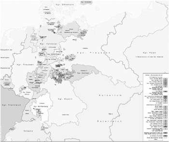
Let us begin with a brief account of the Zollverein.Footnote ⁹ After the defeat of Napoleon in 1815, Germany's political structure was divided into the 39 states of the German Confederation (Deutscher Bund); Figure 1 shows the borders in the year 1820. The confederation consisted of sovereign states in which joint action depended upon unanimity (with Austria and Prussia as the two most powerful polities). Individual states tended to be protectionist and impose a complex set of trade barriers.

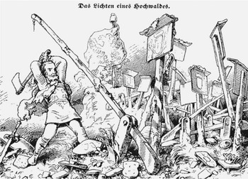
Economists and businessmen were typically opposed to the trade barriers in the Confederation, but they were not the only ones. Indeed, the idea that Germany's numerous customs borders were a hindrance to trade and economic development, as well as political unity, was widely held. Johann Wolfgang von Goethe, for example, told an acquaintance that he looked forward to a time when his luggage would pass unopened through all 36 German states.Footnote ¹⁰ Figure 2 illustrates the prevailing popular sentiments towards customs liberalization at the time: a man axing a customs barrier. Observers frequently drew unfavorable comparisons with other European countries. In the words of List,

The situation is “depressing for [German] men who want to act and trade. With envious eyes they look across the Rhine river, where a large nation [i.e., France], from the [English] Channel to the Mediterranean, from the Rhine to the Pyrenees, from the border with the Netherlands to Italy, engages in trade on open rivers and roads without ever encountering a single customs official.”Footnote ¹¹

Figure 1

Political Borders in Central Europe in the Year 1820

Source: “Mitteleuropa 1820” IEG-Maps (2013).

Although in the minority, there were opponents to economic liberalization, especially in the early 1800s. They included political progressives, who typically did not oppose liberalization per se so much as liberalization under the leadership of Prussia, which they considered politically undesirable.Footnote ¹² Also the nobility of the smaller and mid-sized German states was often hesitant about economic liberalization, mostly because they feared it would herald political changes that would reduce their personal power. However, at times the economic disadvantages of not joining the Zollverein even for the nobility were overwhelming. For example, Ludwig I, the King of Bavaria, strongly supported customs liberalizations with Prussia in 1833, because he feared theexisting customs’ costs would fuel political unrest, thereby leading to a revolution and a loss of his legitimacy (Hahn Reference Hahn and des Deutschen1984, pp. 73–75). Thus, opposition to liberalization waned as everyone came to recognize that Prussian leadership offered the only viable solution for German customs liberalization.

Figure 2

The Zollverein in the Popular Press

Source: Fliegende Blätter, year 1847, volume 6, number 140, page 157; published in Munich.

Burdened with the debts of the Napoleonic wars and the tariffs of Britain, Russia, Austria, France, and the Netherlands, Prussia sought to negotiate international trade treaties while reforming internal tariffs. This was particularly pressing for Prussia because its territories were divided into two, an eastern portion consisting of seven provinces, and a western portion that included the Rhineland provinces and the Ruhr area, each with their own customs. In 1818, the Prussian Customs Union was formed. With few exceptions, internal dues were abolished, and by 1821 only a single tariff for the entire kingdom was levied, while transit dues on goods passing through Prussia were reduced. The Prussian Customs Union was an important model for most of the Zollverein treaties that followed.

States fully surrounded by Prussian territories were the first to sign agreements whereby Berlin would treat these enclaves asif they were her own territory rather than as foreign states that were required to pay import duties. As with all of the following treaties, the signatory states would receive a share of the joint revenue based on population size, and other rights as sovereign states were maintained.

In 1828 Hesse-Darmstadt was the first territorially separate state to join the Prussian Customs Union; Hesse-Cassel followed in 1831. The latter had significant consequences both for east-west and north-south trade. Indeed, only after this agreement could goods flow between the east and west portions of Prussia without an intervening customs border. Moreover, British goods could no longer reach Frankfurt and Germany's south without crossing an external tariff border. In 1834, the Thuringian states, the Kingdom of Saxony, Wurttemberg, and Bavaria joined the augmented Prussian Customs Union which became the Zollverein.Footnote ¹³ At that point the Zollverein had an area of about 163,000 square miles and a population of about 23.5 million people.

Because the Zollverein was a customs union, joining was not a move towards multilateral free trade. Trade diversion was a possible outcome. However, most of trade of the German states at the time was with other German states. A substantial share of the imports from other countries consisted of goods that were not produced in Europe (such as tobacco, sugar, and spices). In fact, between 1833 and 1842, more than 50 percent of the Zollverein revenue was due to such colonial goods (Kolonialwaren; see Dumke Reference Dumke1976, p.92). Therefore, the trade diversion effect of the Zollverein was rather limited.

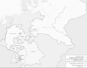
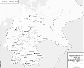
Other states continued to enter after 1834. Baden, Hesse-Nassau, and Frankfurt am Main joined the Zollverein between mid-1835 and early 1836. The entry of Baden, in Germany's far southwest, was important because it allowed goods to move between the two separate areas of Bavaria without a customs’ border (see Figure 3). The entry of Frankfurt allowed manufacturing goods to flow freely up the Main River to Northern Bavaria in exchange for grain. Later on, Brunswick became a member of the Zollverein in 1841, Hanover in 1851, Oldenburg in 1852, Mecklenburg and Luebeck in 1867. Bremen and Hamburg only joined in 1888, after Germany had become politically unified in 1871. Thus, the process of customs' unification unfolded over six decades, from 1821 to 1888.Footnote ¹⁴ Latitude appears to have an important effect on the timing of Zollverein accession. By the year 1836, southern and central states had for the most part joined, whereas many areas in northern Germany stayed outside of the Zollverein until later in the nineteenth century. This provides relevant information for the motives of joining the Zollverein, to which we turn now in greater detail.

Motives for Joining the Customs Union

A number of arguments have been made about the composition and timing of Zollverein accessions. Broad accounts in William O. Henderson (Reference Henderson1959) and Hans-Werner Hahn (Reference Hahn and des Deutschen1984), among others, argue that the expectation of mutual efficiency gains, lower prices, and higher welfare of Prussia (and joining states) were a priori the factors that determined the formation of the Zollverein. A counterargument is that it was the welfare of the feudal lord that counted, not the population at large, and these were not always the same. Although Prussia, as the largest state, may have had the ability to put political pressure on smaller states to join, states retained political sovereignty and Prussia could not force individual states to join against the will of the sovereign. It is well known that even in fully-fledged democracies the gains from free trade might be hard to reap, either because losers oppose the move to free trade or because gains from trade are dissipated in the political process through lobbying or rent-seeking.

In addition, the primary motive driving when individual states joined the Zollverein were clearly idiosyncratic in certain cases. For example, Hanover joined relatively late in part because it was governed in personal union with England, which had no interest in a Prussian led customs union dominating the center of Europe. Other motives that have been proposed are systematic but inconsistent with the evidence (see Dumke Reference Dumke1976). For example, we can easily provide evidence against the argument that the non-joiners preferred tariff rates higher than those Prussia proposed. In fact, Prussia's tariffs on a range of goods, especially colonial goods such as tobacco, tea, and sugar, were higher than the tariffs of many German states before they joined the Zollverein (Dumke Reference Dumke1994, Part III, p. 72). Right before they entered the Zollverein in 1834, for instance, Bavaria and Wurttemberg had ad-valorem tariff rates of 47 percent on Genussmittel (non-essential consumption goods), whereas the tariff rate of the Prussia-Hesse customs union for these goods was 74 percent (Dumke Reference Dumke1976, Table 3.16). Therefore the desire for more protection is unlikely to have been the main reason for not joining the Zollverein.

Figure 3

The Prussian-led Customs Union and the South German Customs Union in 1833

Source: “Zollverträge in Deutschland 22. März 1833” IEG-Maps (2013).

Fiscal reasons are also unlikely to have been paramount. Certainly, it was noted at the time that some of the smaller states with a higher border length to area ratio would find it prohibitively costly to establish and enforce tariff borders have (Kuehne Reference Kuehne1836). If this had been the case we should expect that smaller and highly indebted states would prefer joining the Prussian-led customs union because their fraction of the joint tariff revenue would be larger than the net proceeds they could expect to reap independently. To some extent this is true (Dumke Reference Dumke1976, Chapter 1). Yet, several small and highly indebted states joined the Zollverein relatively late, suggesting others reasons mattered.

We argue that the major motive was market access. In Figures 1 and 3, for simplicity, let us reduce Germany to three regions: the North (e.g., Hannover and Mecklenburg), the Center (Prussia), and the South (Baden and Bavaria). There are some reasons why both the North and the South had an incentive to join the Zollverein. Most importantly membership gave them tariff-free access to the large market of Prussia, including the leading industrial areas of Germany. However, there were also reasons that were specific to the South for joining the Zollverein. Staying out implied that southern exports would have to pay hefty Zollverein tolls before reaching the Baltic or North Sea coast. The coast was important for a number of reasons. First, intermediate goods and machinery from England landed there.Footnote ¹⁵ Moreover, the Baltic and North Sea coast were the main points of access to the sea for Southern states, since the Alps to the south made the trade of high weight-to-value goods such as wheat relatively expensive. Thus, the Southern German states of Baden, Wurttemberg and Bavaria had all joined the Zollverein by 1836; as seen in Figure 4. In contrast, Mecklenburg and the city states of Hamburg and Bremen, which relied heavily on international trade, joined only in 1867 and 1888, respectively. Thus, while it is likely that the benefits of joining would get larger as the customs union expanded, it is also clear that the benefits were not the same for all potential members.

DATA

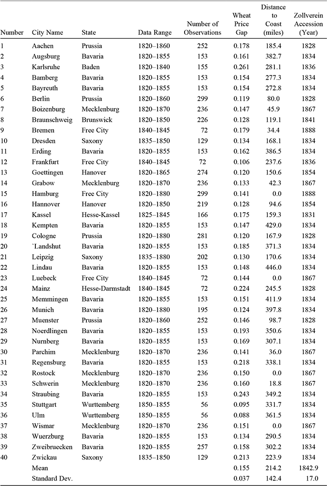
We use the price for wheat in 40 city markets in 14 different German states to analyze trade as it leads to the convergence of prices.Footnote ¹⁶ Table 1 gives an overview of the data. Figure 5 gives the location of the cities. Starting from the average annual wheat price in a given city, we have computed the city's percentage price gap to each of the other cities in the sample for every year where we have information on both cities’ prices.

Figure 4

The Zollverein in the Year 1836

Source: “Deutscher Zollverein 1836” IEG-Maps (2013).

The overall sample period is 1820 to 1880. We left out the first two decades of the nineteenth century because trade was strongly disrupted by wars, and the last two because by 1880 Germany had become politically unified, which may have generated a new environment for trade altogether. The data set includes only every fifth year (1820, 1825, etc.) to reduce the impact of serial correlation on the results. Within the overall sample period of 1820 to 1880, the range of years for which wheat prices are available varies (as given in Table 1); that is, our data set is an unbalanced panel.Footnote ¹⁷ The table also presents the number of price gap observations for each city. For example, Aachen is included as city j or k in 252 cases. Summing across all 40 cities there are 7,140 cases, which corresponds to 3,570 bilateral price gap observations in the sample (out of a possible total of 10,130).

Table 1

Summary Statistics

Notes:

Appendix and author's calculation.

Source:

Factory inspectors' report for 1838 (BPP, 1839).

Figure 5

Price Convergence and the 1834 Customs Liberalizations

Source: Authors' calculation.

Our dependent variable, Trade_jk , is defined as the absolute value of the percentage price gap for wheat between cities j and k in a particular year. This measure is a simple modification of the deviation from the “law of one price.” Suppose Nurnberg exports a unit of wheat to Frankfurt, and Frankfurt charges a customs duty of τ_FN. In the absence of other costs and with competitive markets, the price of wheat in Frankfurt in this period is going to be equal to that in Nurnberg, plus the customs duty, or, the customs duty is equal to the excess of theprice in Frankfurt over that in Nurnberg

(1)

$\[ \begin{array} P_F - P_N = /tau_FN. \end{array} \$

While equation (1) gives the main motivation for studying the impact of customs liberalization—which reduces τ—on price gaps, two points are important. First, the price gap captures more than customs duties. In particular, we expect transport costs, dFN, to affect the price gap between Nurnberg and Frankfurt. The institutional setting matters too, such as the strength of contract enforcement for trades between Nurnberg and Frankfurt.Footnote ¹⁸ Alternatively, if markets are not perfectly competitive there could be mark-ups charged by middlemen; denote the costs capturing this by i_FN . The excess of the price in Frankfurt over that in Nurnberg is then

(2)

$\[ \begin{array} P_F- P_N = /tau_FN /plus d_FN + i_FN, \end{array} \$

which shows that changes in customs duties need not change price gaps one for one. Second, we do not have information on whether the wheat in Frankfurt was shipped from Nurnberg, or from somewhere else. The price in Frankfurt is the minimum across all possible sources:] and the information provided by any given price gap, such as to Nurnberg, gives the lower bound of the bilateral transactions costs:Footnote ¹⁹

(3)

$\[ \begin{array} P_F - P_N /ge /tau_FN + d_FN + i_FN. \end{array} \$

In our sample, the mean absolute value of the percentage price gap between two markets is about 0.18 at the beginning of the sample, and around 0.05 towards the end. Thus the average price gap fell by about 70 percent.Footnote ²⁰ This reflects the dramatic extent of price convergence in Germany over the nineteenth century. This figure is affected by the changing composition of the sample, but these effects appear limited, because the decline for the always present city-pairs is similarly large as in the full sample (73 percent, from 0.11 to 0.03). There is also considerable variation in price gaps across city-pairs in the cross-section. This is in part due to differences in bilateral distance, affecting transport costs, as well as other factors. In the analysis below we will include city-pair fixed effects to address these issues. Further, the decline in price gaps is relatively stronger for initially high price gaps than for low price gaps. At the 10th percentile, the price gap fell from 0.026 at the beginning to 0.016 by the end of the sample period, or, by 38 percent, while at the 90th percentile the price gap fell from 0.39 to 0.09, or by 77 percent.Footnote ²¹

For each city we have recorded the year in which it became part of the Zollverein; this year is listed in Table 1.Footnote ²² Generally, joining the Zollverein meant that barriers for wheat trade between any two of its markets would be equal to zero. Unfortunately, there is no comprehensive information on the levels of tariffs on grain before liberalization. However, in the year 1831 the augmented Prussian customs union charged a specific duty on wheat equivalent to about 7 percent ad valorem (Dumke Reference Dumke1976, Table 3.15). Moreover, the ad valorem equivalents for “products of agriculture” immediately before the formation of the Zollverein in 1834 were about 16 percent in Prussia, 9 percent in Bavaria and Wurttemberg, 8 percent in Baden, and 3 percent in Saxony (Dumke Reference Dumke1976, Tables 3.16). Based on the available information, we estimate that the duties on wheat may have been on average the equivalent of about 10 percent ad valorem before they were reduced to zero in the Zollverein liberalizations.Footnote ²³ Instead of the tariff rates, we will exploit the timing of the move towards zero trade barriers using a dichotomous 0/1 variable.Footnote ²⁴

We eliminated allcity-pairs within the same state, because it is well known that trade and price arbitrage across states is weaker than within states even though the reasons for this are not fully understood.Footnote ²⁵ In the literature, this finding is referred to as the “border effect” (e.g., Shiue Reference Shiue2005).Footnote ²⁶ For each market pair in our sample, we have established using historical maps whether a direct trade route would have to cross any customs borders. If the number of customs borders to be crossed is greater than or equal to one, the variable CustLib_jkt is coded as 0, otherwise it is 1, for each market pair jk and year t.Footnote ²⁷ For example, the customs variable CustLib_jkt turns to 1 for the pair Berlin-Nurnberg in 1834 (when Bavaria joined the Zollverein), while it changes from 0 to 1 for Berlin and Parchim in the year 1867, when Mecklenburg joined the Zollverein. The variable also covers the non-Zollverein customs liberalizations among German states (like the Southern German Union of 1828).

To illustrate our approach, consider the customs liberalizations of the year 1834. In the following analysis, we distinguish the city-pairs for which tariffs were abolished in the year 1834 from the other observations for which customs were liberalized in another year, or not at all during the sample period. In Figure 5 we show the average price gap for both of these groups during the ten years before the 1834 liberalization, versus the ten years after the 1834 liberalization.Footnote ²⁸

The figure shows that before the 1834 liberalization, the average price gap between cities that would reduce their customs barriers was around 0.22, somewhat higher than the value of 0.17 for the cities that would not liberalize in 1834. After the 1834 liberalization, the typical price gap for the liberalizers was around 0.15, down by 0.07, whereas the non-liberalizers’ price gap fell only by 0.01 to about 0.16 on average. Thus, these difference-in-differences results for the 1834 customs liberalization are supportive of the idea that customs liberalizations had a substantial effect on price convergence and trade in nineteenth century Germany. The regression analysis below extends the analysis underlying Figure 5 in three important ways.

First, while the evidence shown in Figure 5 supports the thesis that custom liberalization effect reduced price gaps, there were institutional, fiscal, technological, and other changes affecting cities differently over the nineteenth century that might account for part of the difference in price convergence. In the regression analysis we can account for the major alternative explanations (see in particular Table 2). Second, instead of focusing on the customs liberalization event of 1834, we pool across many such events during the nineteenth century. Further, we focus on price gap changes within each city-pair. Third, and perhaps most importantly the regression analysis that follows corrects for the non-random sequence with which states became members of the Zollverein. As noted previously, the net benefit that each state received from joining the Zollverein depended on its access to international markets. To create a measure of this international trade access, we calculate the distance between each city and the nearest coastal port. Table 1 gives these distances for each of our 40 cities.

Table 2

Reduced-Form Results

Notes:

Notes: Dependent variable is absolute value of percentage price gap between cities j and k; (1820–35) is an indicator variable equal to one for the years 1820 to 1835, zero otherwise; (1840–60) is an indicator variable for the years 1840 to 1860, zero otherwise. French rule: Average of number of years of French rule between 1792 and 1815 in cities j and k. Railway costs: Costs of railway operation between cities j and k in terms of foregone freight, as a function of terrain. Protestant Share: Average of share Protestants in the states in which cities j and k are located. Remote: Average remoteness of cities j and k, defined as difference from the longitude and latitude of the sample mean. Shipping: An indicator variable equal to one if all rivers of the states in which cities j and k are located flow into the Baltic or North Sea, zero otherwise. Coast: An indicator variable equal to one if both cities j and k are in the first quartile of geographic distance to the nearest coast. N = 3,570; p-values based on clustering at the city-pair level in parentheses; all specifications include year- and city-pair fixed effects.

Source:

Authors’ calculation

We also employ measures of a number of other factors that might have affected price gaps between cities (sources and summary statistics are presented in the Appendix). The first is the probability that a given city-pair would be served by a steam railway, an important transportation technology that was introduced in the Zollverein area during the nineteenth century. Using a historical manual (Nicolls Reference Nicolls1878) together with Geographic Information System (GIS) methods, we computed the cost of operating a railway between any pair of cities as a function of the terrain between cities. Second, reductions in transactions costs might have materialized through institutional changes. Daron Acemoglu et al. (2011) show that for a number of German regions, economic growth is increasing in the length of French rule between 1792 and 1815; we compute their length of French rule variable for our city-level sample and include it as a control variable for institutional change. Third, we employ a variable that has been extensively discussed as being related to the viability of a stateas an independent customs area: the ratio of border length to state area (see Kuehne Reference Kuehne1836; Dumke Reference Dumke1976, Reference Dumke1994). The higher the length of the customs border relative to the area of the state, the more costly is it to administer and protect a customs border, and a high border-to-area ratio makes it more likely, according to this argument, that a state would join a larger customs union. Fourth, as a measure of culture as manifested in religious beliefs, we employ the share of Protestants in the states where cities j and k are located. Fifth, we consider the ability to trade by ship, domestically as well as internationally, by employing the following two variables. One is an indicator variable that is equal to one if all rivers that flow through the states in which cities j and k are located empty either into the North Sea or the Baltic Sea. River transport was less costly than either overland or railway transport, and its costs also came down substantially during the nineteenth century in part through the introduction of steam ships. Another variable concerns the position of a given city to engage in international trade; this indicator variable is equal to one if both cities j and k have a distance to the nearest coast that puts them into the lowest quartile in the sample. Other control variables are of a geographic nature (longitude, latitude), and we also employ measures on city population size, from Paul Bairoch, Jean Batou, and Pierre Chevre (Reference Bairoch, Batou and Chevre1988), Jan De Vries (Reference De Vries1984), as well as Wolfgang Keller and Carol Shiue (Reference Goethe and von Goethe2013). We now turn to our empirical results.

EMPIRICAL RESULTS

Our goal is to obtain a valid regression estimate of the impact of customs liberalization (CustLib) on trade (Trade). Let ɛ be the regression error. Correlation between ɛ and customs liberalization would lead to a biased ordinary least squares (OLS) estimate. For example, if the states that expect the largest trade benefits from joining the Zollverein join early, OLS will overestimate the gains from customs liberalization. This gives rise to reverse causation, where the expected gains in Trade determine the decision to liberalize customs. Beyond reverse causation endogeneity through omitted variables is a concern. For example, if Zollverein accession were more likely for relatively small states that get relatively little liberalization gains, OLS would underestimate the impact of the Zollverein.

To solve these econometric problems we use an instrumental variables approach, with relative market access (RDistCoast) as the instrument (for more on the following, see Joshua Angrist and Jörn-Steffen Pischke Reference Angrist and Pischke2009, Chapter 4, especially pp. 152–53). For this strategy to be successful the instrument must first have sufficient power in the sense that conditional on covariates it must be correlated with customs liberalization. This can be tested for as the first-stage correlation, and as we will see, the correlation is strong. Second, the instrument must be valid. For this to be the case the instrument must be as good as randomly assigned. Our instrument is based on geographic features, distance to the nearest coast, which is as close to randomly assigned as one can hope to come in a non-experimental setting. The other condition for the instrument to be valid is that it operates exclusively through the endogenous variable, customs liberalization (this is commonly called the exclusion restriction). This cannot be tested because it involves the unobserved error (one can always estimate a regression residual, but if indeed the analysis is plagued by endogeneity, this residual is not a consistent estimate of the error and hence not useful for applying valid tests). However, a well-known way of gauging the likelihood that the exclusion restriction holds is to extend the reduced form regression (here: the effect of RDistCoast on price gaps) by including other likely determinants of price gaps through which the instrumental variable might operate. We will extensively make use of this approach of providing evidence on the exclusion restriction below (see Table 2).

Our instrumental variable is defined as

(4)

$\[ \begin{array} RDistCoast_jkt = DistCoast_jk/[ODistCoast | Not_Zv_t], \end{array} \$

where DistCoast_jk is defined as the average distance to the nearest North or Baltic Seacoast for cities j and k

(5)

$\[ \begin{array} DistCoast_jk = 0.5 x (DistCoast_j + DistCoast_k. \end{array} \$

The expression [⊘DistCoast|Not_ZV_t ] is the average distance across all market pairs lq to the nearest coast that are not yet part of the Zollverein customs union, as ofyear t:

(6)

$\[ \begin{array} DistCoast | Not I/N/Sigma DistCoast_lg \end{array} \$

where I_lqt is an indicator variable that is one if markets l and q in year t are not yet both part of the Zollverein (and so customs borders do still exist).

Note how this instrumental variable builds on the motives to join the Zollverein that are stressed in historical accounts. First, the numerator of equation (4) captures the fact that a state's accession to the Zollverein was related to the distance to the coast that gave access to international markets. Markets more distant to the coast joined earlier. In particular, joining the Zollverein mattered more for the states in the South of Germany, since that was required for customs-free access to the coast. It is thus not surprising that by 1836, all German states to the south of Prussia had joined the Zollverein. In the first-stage regression, the potentially endogenous variable CustLib is regressed on the instrument RDistCoast—based on earlier arguments we expect a positive coefficient.

Second, the denominator of equation (4) captures the fact that as the Zollverein became larger the net benefit of joining increased over time. Clearly, a larger Zollverein meant more customs-free customers. Moreover, a larger Zollverein raised the chance of having to pay customs duties even when selling to non-Zollverein members because a larger Zollverein customs union meant that it would be more likely that any trade with non-members would have to cross the external Zollverein border. In this way the instrumental variable picks up the fact that The Free City of Frankfurt and Baden, both located moderately far from the coast, joined in 1836, only two years after the Zollverein was founded: it is plausible that the leaders of these states had come to the conclusion that staying outside the union had just become prohibitively costly. This rising cost of staying outside the Zollverein is captured by the instrumental variable because the denominator of RDistCoast declines over time (states far from the coast tend to join early), so that even for a given own distance to the coast the propensity to join the Zollverein is increasing over time.

REDUCED-FORM RESULTS

We now explore the reduced-form regression to shed light on the validity of this instrumental variable. The reduced-form is given by

(7)

$\[ \begin{array} /delta Rails_i, d = /beta_1 Banks_i, d-10 + /beta_2 R_i /beta X_i, d + S_s + e_i, d, \end{array} \$

where the vector X includes city-pair fixed effects and time fixed effects, γ _jk and γ _t , and rdistcoast is equal to the log of RDistCoast, plus one. The fixed effects reduce omitted variable concerns. In particular, the γ _jk imply that identification comes from the changes in price gaps over time within each city-pair.

The relative distance variable is based on geographic characteristics of city markets j and k, as well as on the Zollverein accession decisions of all states. Each individual state's decision has only a small impact on (the denominator) of the instrument, and geography is quite plausibly exogenous, so we estimate equation (7) by OLS. The results are shown in Table 2, first column. A high relative distance to the coast leads to lower price gaps. This is consistent with the idea that city-pairs that are relatively distant from the coast join the Zollverein, and the customs liberalizations of the Zollverein brought down the bilateral price gap.

The remaining columns of Table 2 show extensions of this reduced-form regression. In each column we introduce a different variable, Z

(8)

$\[ \begin{array} Trade_jkt = /gamma_1 rdistcoast_jkt + /gamma_2 Z_jkt +X' /gamma + u_jkt \end{array} \$

where Z is a potential determinant of Trade, which might also be correlated with rdistcoast. Each one of these specifications provides additional evidence on the exclusion restriction, that rdistcoast affects Trade only through its effect on customs liberalization. It is important to distinguish these two features. As we will see, there are several variables that affect Trade in the sense that γ₂ is estimated to be non-zero. In itself, that is not a concern for the instrumental variables strategy. However, if γ₂ is estimated to be non-zero and the coefficient on relative distance γ₁ turns insignificant, that would be evidence that relative distance is strongly correlated with another factor, Z, that affects Trade. In that case, relative distance could not be used as an instrumental variable for customs liberalization because it might fail the exclusion restriction: It would not be clear whether the instrumental variable picks up the Zollverein liberalizations or something related to that other factor, Z.

We first consider institutional change. Many of the German states underwent institutional change as a consequence of French occupation during the times of the French Revolution and in Napoleonic times. These institutional changes tended to be pro-business. In particular, in many areas the “equality before the law” was established, and the influence of craft guilds, which typically would restrict the entry of newcomers in an industry, was curtailed (Acemoglu et al. Reference Acemoglu2011). As a consequence, the institutional change in the German states during the early nineteenth century might affect our instrumental variables strategy: What if these institutional reforms determined which state joined the Zollverein, and not their relative market access as captured by rdistcoast?

A good measure of the depth and the extent of irreversibility of these institutional changes, it turns out, is the length of French rule (Acemoglu et al. Reference Acemoglu2011). We have added the log of the average length of French rule in cities j and k into the reducedform as the next Z variable. The results are shown in column 2 of Table 2. The negative coefficients indicate that longer French rule led to lower price gaps, consistent with the idea that French rule triggered institutional improvements that benefited trade. The test at the bottom of column 2 indicates that, in line with Keller and Shiue (Reference Keller and Shiue2013), French rule is a significant determinant of price gaps. Importantly, the impact of French rule is largely orthogonal to that of the relative distance to the coast; the coefficient on rdistcoast in column 2 is quite similar to that in column 1. Thus, whatever the impact of institutional change on trade might have been, there is no evidence that it will prevent us from estimating the causal impact of the Zollverein on trade using our market access instrument.

According to much of the literature, the introduction of railroads has been second to none in importance for improving trade and causing economic growth in nineteenth century Germany (Fremdling Reference Fremdling1975). It has also been noted that the Zollverein facilitated railway construction. It was easier to agree on the building as well as the location of the railway tracks when all parties were members of the Zollverein, because tariff considerations were removed from the deliberations over routes (Hahn Reference Hahn and des Deutschen1984, p. 93). It is therefore not implausible that railway building both affected trade and was correlated with Zollverein accession. To examine what this means for the Instrumental Variables (IV) strategy, we include a railway measure, namely the GIS-based cost of railway building based on the difficulty of the terrain (from Keller and Shiue Reference Keller and Shiue2013) in the reduced form. According to column 3 of Table 2, railway costs affect price gaps, however they do not much affect the proposed instrument.

In column 4 we include the share of Protestants in the population as an additional Z variable. Protestantism has been proposed as a driver of economic performance (Weber Reference Weber1930), and that may include trade arbitrage. Protestantism is indeed significant as a determinant of price gaps (bottom of column 4). In Germany's North the share of Protestants is larger than in the South. Including Protestantism changes the coefficient on relative distance to the coast.

We also consider the role of remoteness for our results, defined as the geographic location of a particular city-pair relative to the mean of the sample.Footnote ²⁹ Customs liberalization between two relatively isolated markets may matter more than customs liberalization between two markets that each have a multitude of alternative trade partners nearby. Including remoteness also sheds some light on general-equilibrium effects that might be present. Table 2 shows that remoteness is associated with lower price gaps in the sample (column 5).Footnote ³⁰ Including remoteness also reduces somewhat the size of the coefficient on rdistcoast, however, relative distance to coast remains highly significant.

Next, we examine the role of shipping routes, which may be important because the nineteenth century saw the widespread adoption of steam ships in Germany (column 6 of Table 2). The variable Shipping NS is equal to one if the drainage areas in a particular state feed into rivers that flow into either the North Sea or the Baltic Sea (the alternative being that they flow, via the river Danube, into the Black Sea). Including this variable raises (in absolute value) the coefficient on relative distance to coast, which may be due to the geographic flavor of the Shipping NS variable. At the same time, it poses no risk for our instrumental variables strategy.

Another channel that might have affected price gaps is international trade. We know that the nineteenth century saw the arrival of large grain shipments from the United States (O'Rourke and Williamson Reference O'Rourke and Williamson1999). The United Kingdom, in particular, went from importing 0.6 percent of its wheat from the United States in the period 1841 to 1845 to 54.2 percent from the United States during the years 1880–1884 (Dumke Reference Dumke1976, pp. 231–232). Also imports of industrial goods from England might have had a substantial effect on price gaps. An increase in the integration of international markets should primarily affect the coastal areas in Germany, and in column 7 we include an indicator variable for city-pairs that are relatively close to the coast. We estimate that city-pairs located near the coast tended to have higher price gaps, and controlling for that strengthens somewhat the rdistcoast coefficient.

In other analysis we have included latitude, longitude, city size in 1800, and the ratio of border to area as additional variables in the reduced-form equation. These variables were not statistically significant, providing additional support for the exclusion restriction of our instrumental variables approach. Further, we have replacedthe average characteristic of the city-pair with individual variables for the characteristics of each city in the pair;Footnote ³¹ this turns out to lead to similar results. We have also explored the reduced form regression where each variable is interacted with a time trend instead of period fixed effects (for example, the average share of Protestants in cities j and k times year). This more structured approach, which assumes that the effect of Z changes monotonically with time, leads to similar results as those of Table 2 for the relative distance to the coast variable.Footnote ³²

Overall, these results support the assumption that relative distance to the coast exerts its influence on price gaps exclusively through our customs liberalization measure, and thus we proceed with the instrumental variables estimation.

The Impact of Customs Liberalizations on Trade

Our estimate of the impact of customs liberalization on tradeis given by β ₁ in equation 9:

(9)

$\[ \begin{array} Trade_jkt = /beta_1 CustLib_jkt + X^1/beta + /epsiv_jkt \end{array} \$

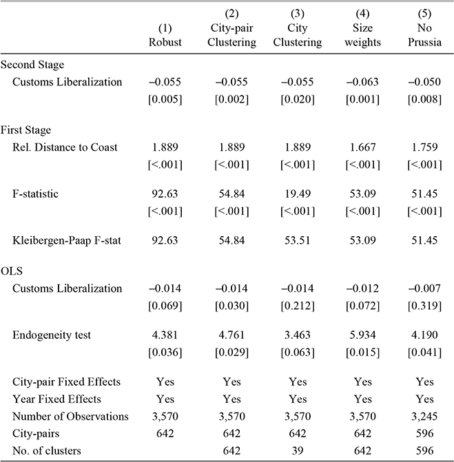
where Customs Liberalization is instrumented by Relative Distance to Coast given in equation (4). The vector X includes year fixed effects (β _t ) and city-pair fixed effects (β _jk ). The method of estimation is two-stage least squares (TSLS). Results are given in Table 3.

The Customs Liberalization coefficient is negative at about −0.05 (column 1), which indicates that customs liberalization has brought down price gaps, by about 28 percent at the mean, and thus improved trade. Inferences in column 1 are based on robust standard errors consistent with arbitrary heteroskedasticity; the p-value of the customs liberalization estimate indicates that it is highly significant at standard levels.

What about the first-stage results? First the F statistic is 90 suggesting the instrument is strong. The Relative Distance to Coast instrument has a positive coefficient. The sign confirms that cities in states that are far away from the coast (such as München) tended to become members of the Zollverein relatively early compared to cities close to the seaboard (such as Hamburg or Bremen).

We also report the OLS estimate of β₁, which would be preferred to TSLS (because of lower variance) if customs liberalizations had been exogenous. The OLS estimate is around–0.015, closer to zero compared to the TSLS estimate. This may be in part because the IV approach addresses the attenuation bias from the measurement error in the 0/1 customs liberalization variable, which does not use the specific size of the tariff cuts in each liberalization. A test of endogeneity indicates that the null of exogeneity can be rejected at standard levels of significance. Because there is evidence that OLS estimates are inconsistent, the discussion will focus on the TSLS estimates.

Table 3

The Impact of the Zollverein Liberalizations

Notes:

Dependent Variable: Absolute value of percentage price gap between cities; p-values in parentheses.

Size weights: Observations are weighted by log average population of cities j and k in year 1800; No Prussia: Observation is dropped if city j is from Prussia. Columns (4) and (5) have p-values based on city-pair clustering.

Source:

Authors' calculation.

Let us now turn to the magnitude of our IV estimate of around −0.05. How reasonable is this? The IV estimate is about three times the size of the OLS estimate. At the same time, the OLS estimate is close to zero, so a tripling of this size is still not a very large number. To put this in perspective, the customs liberalization effect, while sizable, is smaller than the trade impact of railroads in nineteenth century Germany found in Keller and Shiue (Reference Keller and Shiue2013). Moreover, as we noted above the mean price gap in the 1820s is around 0.18, which means that on average customs liberalization has brought price gaps by a little less than one-third during this period (0.05/0.18 equals 0.28). As noted above, the average tariff on agricultural goods was around 10 percent before the customs liberalizations of the Zollverein. In addition, the customs liberalizations coincided with the abolition of non-tariff barriers such as multiple currencies and different units. Our results may also pick up second-round effects, such as stronger cooperation between the different states as a consequence of customs liberalizations, for example in the area of transportation. Given these considerations, the magnitude of this estimate is reasonable.Footnote ³³

CLUSTERING, SIZE

Table 3 also reports results for clustering at the city-pair level. Allowing for arbitrary heteroskedasticity and serial correlation between cross-sectional observations across panels may be important if specific city-pairs are affected by shocks over the nineteenth century. Looking at the results in column 2, however, we see that this clustering does not change the inferences. The third column of Table 3 shows results for clustering at the level of the city, as opposed to the city-pair. Given the bilateral definition of the price gap variable, some dependence between observations at the city level must be present, because if a shock increases the price of wheat in city j, this will affect the price gap of city j with all other cities. Clustering at the city level reduces the precision of the estimates but the customs liberalization coefficient remains significant at better than 2 percent; more importantly, qualitatively the results are unchanged.Footnote ³⁴ We have also considered state-pair clustering as well as clustering by state-pair and year (two-dimensional clustering). Because the decision to join the Zollverein was a political decision made by each state, all cities of a state would typically be affected equally.Footnote ³⁵ Doing so does not affect the qualitative findings of Table 3.

Column 4 shows results from weighing each observation by city size, which gives more weight to the relatively large cities. While the customs liberalization estimate is somewhat larger, overall the results are unchanged.Footnote ³⁶ Further, does the fact that some cities were in Prussia matter for the results? This is an important question because the Zollverein has been seen at times as Prussia's vehicle to achieve both economic and political unification of Germany under Prussia's leadership. In the final column of Table 3, we drop Prussian cities from the sample and again, the results are quite similar to before. Thus, Prussian cities do not appear to play a major role for the results.

Instrumental Variables Results: Robustness

THIRD MARKET AND GENERAL EQUILIBRIUM EFFECTS

By focusing on city-pairs our analysis abstracts from general equilibrium effects, both because of the liberalization of third markets and through the general trends towards protectionism in Europe during the nineteenth century. The Zollverein effect might have been different depending on specific circumstances. For one, while the external tariff of the Zollverein and its precursors on wheat was constant for the period from 1825 to 1851 (Oechselhaeuser Reference Oechselhaeuser1851), the benefit from joining also depended on the level of tariffs between non-Zollverein members. While we do not have the information necessary to fully trace out these effects, the single biggest event in this respect arguably took place in the third quarter of the nineteenth century, when many countries and independent states liberalized their trade. The Zollverein had no external duties on wheat for some time after 1853 (Tracy Reference Tracy1989, p. 87; Henderson Reference Henderson1959, p. 226). Pressure for protection mounted with the arrival of wheat from North America, and in 1879, the German Reichstag reinstated import tariffs on wheat (Tracy Reference Tracy1989, p. 89).

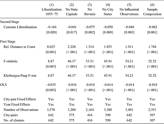
To evaluate the impact of these third-market considerations on the customs liberalization estimate, we present results under the assumption that for the years 1855 to 1875, customs were liberalized between all sample cities, both inside and outside the Zollverein. Column 1 in Table 4 shows that this leads to a larger impact for the customs union. It may be explained in part by the fact that price gaps tended to be higher in the early period, and given that the recoding for 1855 to 1875 leaves less variation in CustLib for the later period, the coefficient rises (in absolute value) because it is primarily identified from the larger changes in price gaps of the early period.

Table 4

Additional Instrumental Variables Results

Notes:

Dependent variable: Absolute value of percentage difference between wheat price in cities j and k; p-values in parentheses based on city-pair clustered standard errors. All specifications include city-pair and time fixed effects. Liberalization 1855–75: Customs Liberalization variable equal to 1 for all city-pairs for all observations for the years 1855–75. No Bavaria: observation is dropped if city j is Bavarian; No City States: Observation is dropped if city j is a city state observation. No influential points based on Cook's Distance. Sample composition: only city-pairs with observations for more than 50 percent of the overall sample period are included.

Source:

Authors’ calculation.

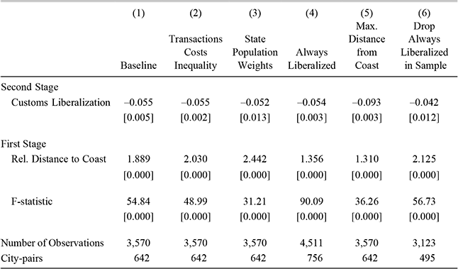
Another way of assessing the importance of third-market effects is to consider the state capitals in the sample. State capitals tend to be particularly important for inter-state trade, both because they account for a relatively high share of all trade and because they may serve as hubs for smaller cities. In column 2 we drop all observations between state capitals from the sample. This leads to a slightly smaller customs liberalization estimate, at −0.041 versus −0.055. Overall, while these results suggest that including third-market effects can lead to either a higher or lower Zollverein estimate, it is unlikely that our analysis gives a gross overestimate of the impact of customs

SAMPLE ROBUSTNESS

The remainder of Table 4 reports estimates for a number of sample restrictions. We begin by eliminating observations with a Bavarian city from the sample. Bavaria, the second largest German state, was closest to being a serious rival for Prussia during the nineteenth century (after Austria-Hungary). Moreover, Bavaria is also highly represented in the sample. In this restricted sample the customs liberalization effect is estimated somewhat higher than before (column 3). Further, the city states of Bremen, Frankfurt, Hamburg, and Luebeck had quite different characteristics than the area states in the sample, and one might be concerned that this might include their response to customs liberalization. It turns out that dropping observations from city states does not change the results by much, see column 4 of Table 4. We have also systematically eliminated the observations that have the most influence on our estimate, as judged by Cook's Distance. Influential observations do not appear to drive our results, see the estimates in column 5. Finally, we have explored the role of the unbalanced sample for these results. A focus on those city-pairs where price information is available for the majority of years during the sample period leads to a similar customs liberalization estimate as for the sample as a whole, see column 6 of Table 4.

OTHER FACTORS

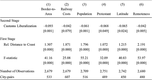
We have also explored the influence of the factors noted in the reduced-form analysis reported in Table 2. Results are given in Table A of the appendix. The first column in Table A gives results for the subsample from which observations with relatively low Border-to-Area ratios are eliminated.Footnote ³⁷ Analogously, in column 2 we drop observations with low Railway Costs while in column 3 observations with low Population are eliminated, and so forth for Latitude and Remoteness.Footnote ³⁸ These results show that the estimation results for the customs liberalization effect are for the most part close to the baseline in column 1.Footnote ³⁹ Further, we have asked whether these results based on wheat prices carry over to other goods. Unfortunately, there are few goods for which price information is as rich as it is for wheat. However, for another good where we have nearly as extensive information on prices, namely rye, we have found also a significant impact of customs liberalizations on bilateral price gaps.

Appendix Table A

The Influence of Other Factors

Notes:

Dependent Variable: Absolute value of percentage price gap between cities; p-values in parentheses. All specifications include time- and city-pair fixed effects; p-values based on clustering at the city-pair level in parentheses. For variable definition, see Table 2.

Source:

Authors' calculation.

Finally, we have found evidence that our results are not significantly affected by the fact that we do not observe the quantities traded, by the different sizes of the German states, and by the particular definition of our instrumental variable based on the average distance of the cities in each city-pairfrom the coast. The interested reader will find these and additional results in Table B of the appendix.

CONCLUDING DISCUSSION

This is the first study, to our knowledge, that incorporates the endogenous effects of accession into an estimate of the economic impact of the Zollverein customs union. We find that the instrumental variable estimate is larger than the OLS estimate that does not take endogenous participation into account. The relatively small OLS effects may explain why the literature has not given much attention to the trade effects of the Zollverein so far.

Beyond its significance as a trade agreement, however, the Zollverein era provides lessons on the impact of economic policy harmonization on the political cohesion between states that are at the core of today's policy debate, not only in Europe but also at a global level. Indeed most trade agreements start with a limited number of early joiners and the participation grows endogenously. For example, there has been a gradual, but marked, expansion in the members of the European Union since it was first established with sixfounding states. As Viner (Reference Viner1950, p. 97) noted, “generalizations about the origin, nature, and consequences of unification of tariffs tend to be based mainly or wholly on the German [i.e., Zollverein] experience.” This holds for membership in multi-lateral free trade agreements such as the General Agreement on Tariffs and Trade (GATT) and now the World Trade Organization (WTO) as well. The differences in when and how specific countries decide to join are important aspects that have often been neglected. They might play a role in explaining the finding that trade agreements of the more recent past have not raised trade (Rose Reference Rose2004). Recent research has sought to identify the general characteristics of countries that choose to join trade agreements, finding larger trade agreement effects after taking into account income and other broad characteristics into account (Baier and Bergstrand Reference Baier and Bergstrand2007; Egger et al. Reference Egger, Larch, Staub and Winkelmann2011). None of these characteristics are specific to the particular trade agreement being looked at. In contrast to these studies, our analysis of the case of nineteenth century Germany captures the motives for joining a specific trade agreement, the Zollverein, at a new level of detail and is targeted to the specific historical context of the agreement.

Appendix Table B

Notes:

Dependent Variable: Absolute value of percentage price gap between cities; p?values in parentheses; (2) Regression weight relatively low if world wheat price low and close to coast, high if far from coast and world price high; (3) Regression with state population in year 1816 as weights; (4) Include city-pairs between which customs was always liberalized; (5) Instrumental variable computed from maximum instead of average distance across cities j and k; (6) Drop from sample if all price gap observations in sample only during customs-liberalized years. All specifications include time- and city-pair fixed effects; p-values based on clustering at the city-pair level in parentheses.

Source:

Authors’ calculation.

Our results also recast the debate on the impact of the Zollverein for economic growth in Germany. At first the contribution of the Zollverein to Germany's industrial take-off was widely accepted as a given (Henderson Reference Henderson1959). Post-war economic history called this into question, although the revisionist thinking was not always backed up by compelling empirics. In this paper we show that historically, market access was fundamentally important to regional incentives, and accounting for it is crucial for uncovering the major Zollverein contribution for nineteenth century German trade. Along these lines, this paper takes the first step towards resurrecting the role of the Zollverein for German industrial development more generally. The role of market access for economic performance has been central in recent work on trade and regional economics, such as the work of Paul Krugman and others (e.g., Fujita, Krugman, and Venables Reference Fujita, Krugman and Venables1999). Market access can have an important impact on the locations of where manufacturing centers arise. Our finding of a substantial Zollverein effect suggests that trade policy may have played an important role for other economic developments within the German region in the nineteenth and twentieth centuries, including where German manufacturing centers arose.

Appendix: Data Definitions and Sources

Wheat Prices The two most important sources for information on wheat prices used in this paper are Carol Shiue and Wolfgang Keller (Reference Shiue and Keller2007) and Georg K.L. Seuffert (Reference Seuffert1857). The former covers markets in Bavaria and Mecklenburg, while the latter provides information on markets in Baden, Brunswick, Hesse-Darmstadt, Hesse-Cassel, Saxony, and Wurttemberg. The wheat prices for Prussian markets were provided by Kopsidis (Reference Kopsidis2002). Additional sources to expand the coverage are Fremdling and Hohorst (Reference Fremdling and Hohorst1979), Hans-Jürgen Gerhard and Karl Heinrich Kaufhold, et al. (Reference Gerhard and Kaufhold1990) for Prussia, and Vierteljahrshefte (1935) for Berlin, Cologne, Hamburg, Leipzig, and Munich.

As noted in the text, while virtually all price data are official records of the price of wheat at market days, in some cases the annual average price is computed from monthly prices by us (e.g., for the Bavarian cities), while in other cases the annual average price is given in the source (e.g.,for Berlin). We have computed the annual average price as the simple arithmetic average of the monthly prices; using quantity weights, which are available for some markets, for example Munich, makes little difference. Since neither quantity nor monetary units were standardized in the German states during the nineteenth century, conversion rates are required for our analysis of absoluteprice differences, and all prices are converted into Bavarian Gulden per Bavarian Schaeffel. The conversion factors are taken from the original sources (see Shiue and Keller Reference Shiue and Keller2007) as well as from Seuffert (Reference Seuffert1857). Specifically, from the latter we have (p. 351):

Zollverein Membership A list with the dates of when states joined the Zollverein is givenin Dumke (Reference Dumke1976, pp. 98–99). The customs liberalization variable CustLib is constructed usingthe historical maps at IEG (2013); CustLib_jkt is equal to 1 if in year t there was at least one customs border between cities j and k, and 0 otherwise.

Railway Cost Based on the capacity of a steam locomotive to haul freight as function of terrain (Nicolls Reference Nicolls1878) we construct a cost function, and use a 90 meter × 90 meter GIS map of the relevant area in central Europe and the ArcGIS least-cost distance module to compute the least-cost routes, as well as the associated costs of those routes, from each city to all other cities in the sample. The railway variable in Table 2 is the railway cost as defined in the paper divided by the bilateral geographicdistance. All geographic distances in this paper use the Haversine formula. See Keller and Shiue (Reference Keller and Shiue2013) for more details.

French Occupation Length of the French occupation during revolutionary and Napoleonic times, source Acemoglu et al. (Reference Acemoglu2011).

Border-to-Area log of average of border length to state area. Source: von Viebahn (Reference von Viebahn1858, p. 520) and Dumke (Reference Dumke1976, p. 97). Mean −0.60, standard deviation 0.76.

Population log of the average population of cities j and k in the year 1800. Source: Bairoch, Batou, and Chevre (Reference Bairoch, Batou and Chevre1988), De Vries (Reference De Vries1984), and estimates of Keller and Shiue (Reference Keller and Shiue2013). Mean 2.90, standard deviation 0.92.

Protestantism Average of the share of Protestants in the states where cities j and k are located, in the year 1858. Source: Georg von Viebahn (Reference von Viebahn1862, p. 337). Mean 65.05, standard deviation17.87.

Latitude Maximum of latitude of cities j and k, from www.maporama.com, accessed November 2008. Mean 52.43, standard deviation 1.37.

Longitude Maximum of longitude cities j and k, from www.maporama.com, accessed November 2008. Mean 11.55, standard deviation 1.16.

Shipping NS Equal to 1 if for both cities j and k all rivers through the states in which j and k are located empty either in the North Sea or Baltic Sea, and 0 otherwise. The third alternative is rivers flowing into the Danube and then the Black Sea. Source: Computed from information in von Viebahn (Reference von Viebahn1858, p. 256). Mean 0.16, standard deviation 0.37

Coast This variable is equal to one if both cities j and k have a distance to the nearest coast that puts them into the lowest quartile in the sample. Source: Latitude and longitude information of the cities and the closest points on a coast relative to them, in terms of direct geographic distance (using the Haversine formula). Mean 0.04, standard deviation 0.20.

Footnotes

We thank Rainer Fremdling, Florian Ploeckl, two referees and the editor, as well as seminar audiences at Berkeley, CEPR ERWIT, the Cliometric Society, Colorado, Harvard, Lund, the NBER, the Philly Fed, and Yale for useful comments. Michael Kopsidis provided us with data. NSF support under grant numbers SES 0453040 and 1124426 is gratefully acknowledged. This paper was written in part while both authors were National Fellows at Hoover Institution, Stanford University, whose hospitality is acknowledged as well.

1 For historical overviews of the Zollverein, see Henderson (Reference Henderson1959), Dumke (Reference Dumke1976), and Hahn (Reference Hahn and des Deutschen1984).

2 The petition is printed in German in von Eisenhart, Rothe, and Ritthaler (Reference von Eisenhart Rothe and Ritthaler1934, pp. 320–24).

3 Price data contains important information on trade and its effects (e.g., Stolper and Samuelson Reference Stolper and Samuelson1941) and has been extensively applied in the literature (O'Rourke and Williamson Reference O'Rourke and Williamson1999). Information on the volume of trade becomes available for these areas only at a later time (Wolf, Schulze, and Heinemeyer Reference Nikolaus, Schulze and Heinemeyer2011).

4 On the endogeneity of trade agreements, see the Baldwin (Reference Baldwin1993), Baldwin and Jaimovich (Reference Baldwin and Jaimovich2012).

5 For example, the 1831 accession of Hesse-Cassel to the Prussia-led customs union meant that all goods shipped between southern Germany and the northern ports of Hamburg and Bremen had to pass the external barrier of the Prussian-led customs union (Keller and Shiue Reference Keller and Shiue2008); see also Figure 4. Ploeckl (Reference Ploeckl2010a) presents a bargaining model for the formation of the Zollverein as well as additional evidence on the importance of international trade access.

6 On endogeneity in a related setting, see Ritschl and Wolf (Reference Ritschl and Wolf2003).

7 This overall beneficial effect for trade of the Zollverein is consistent with the finding that within individual German states, some regions benefited more while others benefited less (Ploeckl Reference Ploeckl2010b, Reference Ploeckl2012).

8 Other work that has considered in particular railroads includes Keller and Shiue (Reference Keller and Shiue2008, Reference Keller and Shiue2013).

9 On the following, see also Henderson (Reference Henderson1939), Hahn (Reference Hahn and des Deutschen1984), as well as Dumke (Reference Dumke1976), Ploeckl (Reference Ploeckl2010a).

10 Goethe in conversation with Eckermann in the year 1828; see Goethe (Reference Goethe and von Goethe1828).

11 Reprinted in German in von Eisenhart, Rothe, and Ritthaler (Reference von Eisenhart Rothe and Ritthaler1934, pp. 320–24).

12 Several German states had by then adopted constitutions, which Prussia had not.

13 The South German Customs Union was formed in 1828 and consisted of Wurttemberg and Bavaria.

14 Austria did not become a member of the Zollverein. Reasons for this include Austria's relatively protectionist stance towards trade and her competition with Prussia.

15 For example, the quantity of pig iron imported by Prussia in 1822, 32,000 Zentner, rose by a factor of about 384 to 12,278,000 Zentner by the year 1873, the quantity imported by the Deutsche Reich (Dumke Reference Dumke1994, Part II, p. 61); most of this was imported from England (Dumke Reference Dumke1994, Part II, p. 37). England exported also machinery to Germany; for example, the locomotive factory Robert Stephenson and Company sold in 1835 a locomotive that would become the first steam locomotive to run in the German lands, between Nurnberg and Fuerth. More machinery from England was imported in the German lands after the end of the export ban on textile machinery in 1843 (Burly Reference Burly1960, p. 28).

16 The underlying source of these annual wheat prices are typically the officially recorded prices on market days, usually one per week. The reason for the government's interest in grain prices was that price spikes could produce food riots that might threaten the sovereign's legitimacy. In some cases, our sources provide the annual average while in other cases it is computed by the authors; see also the Appendix.

17 We have no reason to believe that sample selection matters for our results; a focus on citypair observations that are in the sample with relatively high frequency leads to similar results, as noted in our discussion of the Table 4 results below.

18 In addition, there could be other transactions costs as well, such as uncertainty, losses due to risks in shipping or insurance, or quality variations in wheat.

19 Price gaps vary in how informative they are on bilateral transactions costs. A plausible hypothesis is that for two markets close to the coast, which might be both importing wheat from a third market, equation (3) holds only with an inequality. Exploring this empirically, we do not find that it alters the results significantly; see Table B, (2). This suggests that systematic reasons for equation (3) holding with equality have no strong effect on our results.

20 We compute the absolute value because the local price of wheat is affected by weather, and from year to year it might change which city is the low-cost producer.

21 Given this difference, we do not necessarily expect that customs liberalizations have the same effect throughout the sample.

22 For the Prussian cities in the sample, we give the year 1828, which is the earliest year at which another state became part of the Prussian-led Zollverein. Customs liberalizations that did not involve Zollverein accession are discussed in section 4.

23 Tariff levels on manufactured goods in 1834 ranged from 20.9 percent in Bavaria and Wurttemberg to 2.1 percent in Saxony across the same four areas, and they ranged from 18.9 percent in Prussia-Hesse to 5.1 percent in Saxony for intermediate goods and materials. With these figures—all ad-valorem equivalents—tariff levels for agricultural goods on the one hand, and manufactured and intermediate goods on the other may have been quite similar on average. In contrast, tariffs on Genusmittel (non-necessities) where higher; in Prussia-Hesse for example, as noted earlier, they were 74 percent (Dumke Reference Dumke1994, Part III, p.72).

24 In a few cases, the time of the Zollverein accession does not coincide with the year in which tariffs on grain were eliminated. For example, the tariffs between Bavaria and the augmented Prussian customs union were eliminated in 1829, four years before the Zollverein treaty. We focus nevertheless on the Zollverein accession date, because arguably this played the key role in terms of commitment.

25 The number of such city-pairs is 114, eliminating connections between east and west Prussia. Even within states the strength of arbitrage varies along jurisdictional boundaries, see Schulze and Wolf (Reference Schulze and Wolf2009). At the same time, we have confirmed that in our context, including the cities between which customs barriers were always absent does not significantly affect our estimate of the impact of customs liberalization; see Table B, (4).

26 These excluded observations are typically within-state market pairs.

27 While this definition means we could be missing the cumulative effect of multiple customs borders, we have explored the issue and found that no significant difference in the customs liberalization effect for single versus multiple customs liberalizations.

28 Recall that we employ data every five years, so the pre-period years are 1820, 1825, and 1830, while the post-period years are 1835, 1840, and 1845.

29 If lat_jk and long_jk are the average latitude and longitude of city-pair jk, then we define rem_jk = as city-pair jk's remoteness, where and are the sample averages across all lat_jk and long_jk , respectively.

30 Anderson and van Wincoop (Reference Anderson and van Wincoop2003) have shown in a gravity equation framework that such general equilibrium effects are picked up by so-called multilateral resistance terms, which perform the same function as our remoteness variable. In short, from their analysis one should expect Australia and New Zealand, for example, to trade more with each other than two similarly sized countries in the center of Europe that are equally far apart. This is because Australia and New Zealand are more remote from other potential trade partners than the two European countries. In our analysis of bilateral transactions costs, more trade corresponds to lower transactions costs, and therefore our finding that transactions costs tend to be lower between relatively remote citypairs is in line with such general equilibrium effects.

31 For example, Protestantism in city j and Protestantism in city k separately, instead of the variable 0.5 × (Protestantism in city j + Protestantism in city k).

32 We have also included bilateral geographic distance in the reduced form, interacted with period dummies, as a control for differential changes in transport costs for short- versus longdistance trade. The results are similar.

33 It is worth keeping in mind that we estimate a local average treatment effect, namely the impact of customs liberalization on price gaps for the set of city-pairs that were induced to liberalize customs as captured by our instrumental variable. This estimate has the advantage that it addresses endogeneity and, consequently, the estimate is consistent. At the same time, the (global) average treatment effect of customs liberalizations is something we leave for future work.

34 We also report the more general Kleibergen and Paap (KP) F-statistic in addition to the usual first-stage F-statistic. The KP is often compared with Stock and Yogo's (Reference Stock, Yogo, Andrews and Stock2005) critical values to gain additional information on the strength of the first stage (even though Stock and Yogo's critical values are for the i.i.d. case). In our case, the KP statistic is far larger than Stock and Yogo's critical values, confirming that the first stage is strong.

35 This was not always the case. For example, the South German Customs Union abolished tariffs between Württemberg and Bavaria in the year 1828. Nonetheless, the Bavarian town of Zweibruecken continued to face customs borders in its trade with Württemberg because Zweibruecken was located in a geographically disjoint part of Bavaria (Palatinate, or “Pfalz”), see Figure 3.

36 We have also experimented with adjusting for the different population sizes at the state level; for example, Prussia had more than 10 million inhabitants in the early nineteenth century, compared to about 40,000 in the Free City of Luebeck. Weighing each city-pair observation by average state population in 1816 yields an estimate of −0.052, similar to the unweighted results of −0.005, see Table B, (3).

37 Specifically, the first quartile of the sample in terms of Border-to-Area ratio is dropped.

38 The results for Longitude are similar and available from the authors upon request.

39 The exception to this is Border-to-Area, where it appears that the customs estimate is relatively large for high border-to-area observations, compared to the average city-pair in the sample. To the extent that the high Border-to-Area observations are city state observations, though, we have seen in Table 4 that eliminating city state observations does not lead to a very different customs liberalization estimate.

References

REFERENCES

Acemoglu, Daron et al. “The Consequences of Radical Reform: The French Revolution.” American Economic Review 101, no. 7 (2011): 3286–307.Google Scholar

Anderson, James E., and van Wincoop, Eric. “Gravity with Gravitas: A Solution to the Border Puzzle.” American Economic Review 93, no. 1 (2003): 170–92.CrossRef Google Scholar

Angrist, Joshua, and Pischke, Jörn-Steffen. Mostly Harmless Econometrics. An Empiricist's Companion. Princeton University Press, 2009.Google Scholar

Baier, Scott, and Bergstrand, Jeffrey, “Do Free Trade Agreements Actually Increase Members’ International Trade?” Journal of International Economics 71, no. 1 (2007): 72–95.Google Scholar

Bairoch, Paul, “European Trade Policy, 1815–1914.” In The Cambridge Economic History of Europe, Vol. 8, edited by Mathias, Peter and Pollard, Sidney, pp. 1–160. Cambridge: Cambridge University Press, 1989.Google Scholar

Bairoch, Paul, Batou, Jean, and Chevre, Pierre. The Population of European Cities from 800 to 1850: Data Bank and Short Summary of Results. Geneva: Librairie Droz, 1988.Google Scholar

Baldwin, Richard, “A Domino Theory of Regionalism.” CEPR Discussion Paper No. 857, CEPR, 1993.Google Scholar

Baldwin, Richard, and Jaimovich, Dany. “A Free Trade Agreements Contagious?”Journal of International Economics 88, no. 1 (2012): 1–16.Google Scholar

Burly, J.P.T. “The Zenith of European Power, 1830–1870.” Volume 10 in the New Modern Cambridge History. Cambridge: Cambridge University Press, 1960.Google Scholar

De Vries, Jan. European Urbanization 1500–1800. Cambridge: Harvard University Press, 1984.Google Scholar

Dumke, Rolf H. “The Political Economy of German Economic Unification: Tariffs, Trade and Politics of the Zollverein Era.” Ph.D. Dissertation, University of Wisconsin-Madison, 1976.Google Scholar

Dumke, Rolf H. “German Economic Unification in the 19^th Century: The Political Economy of the Zollverein.” Working Paper, Universitaet der Bundeswehr, Muenchen, 1994.Google Scholar

Egger, Peter, Larch, Mario, Staub, Kevin E., and Winkelmann, Rainer. “The Trade Effects of Endogenous Preferential Trade Agreements.” American Economic Journal: Economic Policy 3, no. 3 (2011): 113–43.Google Scholar

Federico, Giovanni, “When Did European Markets Integrate?” European Review of Economic History 15, no. 1 (2011): 93–126.Google Scholar

Federico, Giovanni, and Persson, Karl Gunnar, “Market Integration and Convergence in the World Wheat Market, 1800–2000.”Discussion Paper, University of Copenhagen, 2010.Google Scholar

Federico, Giovanni, and Tena, Antonio. “Was Italy a Protectionist Country?” European Review of Economic History 2, no. 1 (1998): 73–97.Google Scholar

Fremdling, Rainer. Eisenbahnen und deutsches Wirtschaftswachstum 1840–1879. Dortmund, 1975.Google Scholar

Fremdling, Rainer,and Hohorst, Gerd.“MarktintegrationderpreussischenWirtschaft im 19. Jahrhundert-Skizze eines Forschungsansatzes zur Fluktuation der Roggenpreise zwischen 1821 und 1865.”In Industrialisierung und Raum edited by Richard Tilly and Rainer Fremdling, 56–101. Stuttgart: Klett-Cotta, 1979.Google Scholar

Fujita, Masahisa, Krugman, Paul, and Venables, Anthony.The Spatial Economy. Cities, Regions, and International Trade. Cambridge: MIT Press, 1999.CrossRef Google Scholar

Gerhard, Hans-Jürgen, Kaufhold, Karl Heinrich et al. , Preise im vor- und frühindustriellen Deutschland: Grundnahrungsmittel. Gottingen: O. Schwartz, 1990.Google Scholar

Goethe, Johann von Goethe, Wolfgang. Conversation with Eckermann on Oct. 23, 1828. Leipzig: F.W.v. Biedermann, 1909–1911. Accessed February 27, 2013 online at http://www.zeno.org.Google Scholar

Hahn, Hans-Werner. des Deutschen, Geschichte Zollvereins, Vandenhoeck & Ruprecht: Gottingen, 1984.Google Scholar

Henderson, William O. The Zollverein. Originally published in 1939. Cambridge, UK: Cambridge University Press, 1959.Google Scholar

IEG-Maps. Server fur digital Karten am Institut fur Europaische Geschichte, Mainz, 2013. Accessed February 2013 http://www.ieg-maps.uni-mainz.de/ Google Scholar

Jacks, David, “Intra- and International Commodity Market Integration in the Atlantic Economy, 1800–1913.” Explorations in Economic History 42, no. 3 (2005): 381–413.Google Scholar

Keller, Wolfgang, and Shiue, Carol. H. “Tariffs, Trains, and Trade: The Role of Institutions versus Technology in the Expansion of Markets.” NBER Working Paper No. 13913, Cambridge, MA, April 2008.Google Scholar

Keller, Wolfgang, and Shiue, Carol. H. “The Link Between Fundamentals and Proximate Factors in Development.” NBER Working Paper No. 18808, Cambridge, MA, February 2013.Google Scholar

Kopsidis, Michael, “The Creation of a Westphalian Rye Market 1820–1870: Leading and Following Regions, an Co-Integration Analysis.” Jahrbuch fur Wirtschaftsgeschichte 43, no. 2 (2002): 85–112.Google Scholar

Kuehne, Ludwig. Ueber den deutschenZollverein, Duncker & Humblot, 1836.Google Scholar

Nicolls, William J. The Railway Builder, Philadelphia, 1878.Google Scholar

Oechselhaeuser, Wilhelm. Der Zollverein, Seine Verfassung, sein handels-politisches System und die Entwicklung der Tarifsaetze seit 1818, Frankfurt: Heinrich Ludwig Broenner, 1851.Google Scholar

O'Rourke, Kevin, and Williamson, Jeffrey G..Globalization and History, Cambridge: MIT Press, 1999.Google Scholar

Persson, Karl Gunnar.Grain Markets in Europe, 1500–1900: Integration and Deregulation, Cambridge University Press, 1999.Google Scholar

Ploeckl, Florian, “The Zollverein and the Formation of a Customs Union.” ESH Working Paper No. 84, Oxford University, 2010a.Google Scholar

Ploeckl, Florian, “Borders, Market Access and Urban Growth; the Case of Saxon Towns and the Zollverein.” Institut d'Economia de Barcelona Working Paper No. 42, 2010b.Google Scholar

Ploeckl, Florian, “The Internal Impact of a Customs Union; Baden and the Zollverein.” Mimeo, Oxford University, 2012.Google Scholar

Ritschl, Albrecht, and Wolf, Niko, “Endogeneity of Currency Areas and Trade Blocs: Evidence from the Inter-War Period, CEPR Discussion Paper No. 4112, CEPR, November 2003.Google Scholar

Rose, Andrew, “Do We Really Know That the WTO Increases Trade?” American Economic Review 94, no. 1 (2004): 98–114.Google Scholar

Schulze, Max-Stephan, and Wolf, Niko. “On the Origins of Border Effects: Insights from the Habsburg Empire.” Journal of Economic Geography 9, no. 1 (2009): 117–36.Google Scholar

Seuffert, Georg K. L. Statistik des Getreide- und Viktualien-Handels im Konigreiche Bayern mit Berucksichtigung des Auslandes, J. G. Weiss, Munich, 1857.Google Scholar

Shiue, Carol H. “From Political Fragmentation Towards a Customs Union: Border Effects of the German Zollverein, 1815 to 1855.” European Review of Economic History 9, no. 2 (2005): 129–62.Google Scholar

Shiue, Carol H., and Keller, Wolfgang. “Markets in China and Europe on the Eve of the Industrial Revolution.” American Economic Review 97, no. 4 (2007): 1189–216.Google Scholar

Staiger, Douglas, and Stock, James. “Instrumental Variable Estimation with Weak Instruments.” Econometrica 65, no. 3 (1997): 557–86.Google Scholar

Stock, James, and Yogo, Motohiro. “Testing for Weak Instruments in Linear IV Regressions.” In Identification and Inference for Econometric Models: Essays in Honor of Thomas Rothenberg, Andrews, Donald W.K. and Stock, James H. (eds.), 80–108. Cambridge: Cambridge University Press, 2005.Google Scholar

Stolper, Wolfgang F., and Samuelson, Paul. A. “Protection and Real Wages.” Review of Economic Studies 9, no. 1 (1941): 58–73.Google Scholar

Tracy, Michael. Government and Agriculture in Western Europe 1880–1988, 3rd edition, New York: New York University Press, 1989.Google Scholar

Uebele, Martin, “Demand Matters: German Wheat Market Integration 1806–1855 in a European Context.” Working Paper, University of Muenster, 2010.Google Scholar

Vierteljahrshefte.Vierteljahrshefte zur Statistik des Deutschen Reichs, Year 1935, Germany, StatistischesReichsamt, 1935.Google Scholar

Viner, Jacob. The Customs Unions Issue. New York: Carnegie Endowment for International Peace, 1950.Google Scholar

von Eisenhart Rothe, Wilfried, and Ritthaler, Anton. Vorgeschichte und Begrundung des deutschen Zollvereins: 1815–1834, Berlin 1934.Google Scholar

von Viebahn, Georg.Statistik des Zollvereinten und nordlichen Deutschlands, Erster Theil, Georg Reimer Verlag, Berlin, 1858.Google Scholar

von Viebahn, Georg, Statistik des Zollvereinten und nordlichen Deutschlands, Zweiter Theil (Bevolkerung, Bergbau, Bodenkultur), Georg Reimer Verlag, Berlin, 1862.Google Scholar

Weber, Max. The Protestant Ethic and the Spirit of Capitalism. Originally published in 1905. Routledge: London, 1930.Google Scholar

Nikolaus, Wolf, Schulze, Max-Stephan, and Heinemeyer, Hans-Christian. “On the Economic Consequences of Peace: Trade and Borders After Versailles.” The Journal of Economic History 71, no. 4 (2011): 915–49.Google Scholar

Figure 1Political Borders in Central Europe in the Year 1820

Source: “Mitteleuropa 1820” IEG-Maps (2013).

Figure 2The Zollverein in the Popular Press

Source: Fliegende Blätter, year 1847, volume 6, number 140, page 157; published in Munich.

Figure 3The Prussian-led Customs Union and the South German Customs Union in 1833

Source: “Zollverträge in Deutschland 22. März 1833” IEG-Maps (2013).

Figure 4The Zollverein in the Year 1836

Source: “Deutscher Zollverein 1836” IEG-Maps (2013).

Table 1Summary Statistics

Figure 5Price Convergence and the 1834 Customs Liberalizations

Source: Authors' calculation.

Table 2Reduced-Form Results

Table 3The Impact of the Zollverein Liberalizations

Table 4Additional Instrumental Variables Results

Appendix Table AThe Influence of Other Factors

Appendix Table B

Article contents

Endogenous Formation of Free Trade Agreements: Evidence from the Zollverein's Impact on Market Integration

Abstract

Information

Germany's Nineteenth Century Trade: The Zollverein Treaties

Motives for Joining the Customs Union

DATA

Notes:

Source:

Notes:

Source:

EMPIRICAL RESULTS

REDUCED-FORM RESULTS

The Impact of Customs Liberalizations on Trade

Notes:

Source:

CLUSTERING, SIZE

Instrumental Variables Results: Robustness

THIRD MARKET AND GENERAL EQUILIBRIUM EFFECTS

Notes:

Source:

SAMPLE ROBUSTNESS

OTHER FACTORS

Notes:

Source:

CONCLUDING DISCUSSION

Notes:

Source:

Appendix: Data Definitions and Sources

Footnotes

References

REFERENCES

Save article to Kindle

Save article to Dropbox

Save article to Google Drive

Reply to: Submit a response

Your details

You have entered the maximum number of contributors

Conflicting interests