Implications
Results of the present study may be contemplated as guidelines both for upcoming studies and for selection programs accounting for count traits involved on in vitro embryo production processes. In most cases, count variables have been analyzed after logarithmic scale transformation. By assessing the goodness of fit of different Bayesian models, it was possible to suggest novel strategies that yield reduced bias when modeling those types of traits within animal breeding purposes.
Introduction
Technologies such as multiple-ovulation followed by embryo transfer and, more recently, in vitro embryo production allowed breeders to continuously increase selection pressure and reduce generation intervals (Bols et al., Reference Bols, Goovaerts, Jorssen, Petro, Langbeen and Leroy2012). Bos indicus cattle breeds present an outstanding performance on in vitro embryo production technologies (Viana et al., Reference Viana, Siqueira, Palhao and Camargo2012; Rodrigues, Reference Rodrigues2015) and genetic analysis for in vitro embryo production traits could help to maintain high productivity indices.
Traits of interest in embryo production processes are mainly defined as counts. In the context of animal breeding, major strategies to model embryo yield are based in variable transformation (Peixoto et al., Reference Peixoto, Pereira, Bergmann, Penna and Fonseca2004; Merton et al., Reference Merton, Ask, Oonkundi, Mullaart, Collenbrander and Nielen2009), by assuming normality of the sampling for embryo yield (Tonhati et al., Reference Tonhati, Lôbo and Oliveira1999). However, natural distributions for count data are often given by Poisson (POI) (Rodrigues-Motta et al., Reference Rodrigues-Motta, Gianola and Heringstad2007; Vazquez et al., Reference Vazquez, Weigel, Gianola, Bates, Perez-Cabal, Rosa and Chang2009b and Reference Vazquez, Pérez-Cabal, Heringstad, Rodrigues-Motta, Rosa, Gianola and Weigel2012; Ayres et al., Reference Ayres, Pereira, Boligon, Silva, Schenkel, Roso and Albuquerque2013; Abdolahi-Arpanahi et al., Reference Abdolahi-Arpanahi, Peñagaricano, Aliloo, Ghiasi and Urioste2013) and zero-inflated Poisson (ZIP) (Naya et al., Reference Naya, Urioste, Chang, Rodrigues-Motta, Kremer and Gianola2008; Rodrigues-Motta et al., Reference Rodrigues-Motta, Gianola, Heringstad, Rosa and Chang2010) distributions.
Studies suggest the presence of genetic component influencing embryo production in cattle (Merton et al., Reference Merton, Ask, Oonkundi, Mullaart, Collenbrander and Nielen2009; Jaton et al., Reference Jaton, Koeck, Sargolzaei, Malchiodi, Price, Schenkel and Miglior2016; Perez et al., Reference Perez, Peixoto, Bruneli, Ramos and Balieiro2016), however, no model comparison has been reported. The goal of the present study was to identify the best fitting model, which yields the least amount of bias for count traits related to in vitro embryo production. Models assuming different distributions (Gaussian, POI and ZIP) for the observations were compared and discussed under a genetic evaluation framework.
Material and methods
Data
A total of 5716 records from ovum pick-up and in vitro embryo production procedures were analyzed, in 1205 Guzerá breed female donors, daughters of 262 sires. Sessions occurred between March 2003 and July 2013, in 16 herds. Animals were 1 to 20 years old at the ovum pick-up (OPU) moment. The pedigree file used to estimate relationship between the 1 205 donors (phenotyped animals) included 6850 individuals. The number of sessions varied from 1 to 49 per donor and the intervals between OPU sessions of the same donor varied from 7 to 120 days. A total of 147 different bulls (semen) were used for the in vitro fertilization process.
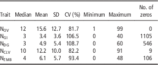
Traits analyzed in this study were: number of viable oocytes (NOV), number of grade I oocytes (NGI), number of degenerated oocytes (NDG), number of cleaved embryos (NCLV) and number of viable embryos produced (NEMB). Table 1 shows the descriptive statistics of these traits.
Median, means, standard deviations (SD), coefficient of variation (CV), minimum and maximum values and the number of 'zero' observations in the dataset for the analyzed traits

NOV=number of viable oocytes; NGI=number of grade I oocytes; NDG=number of degenerated oocytes; NCLV=number of cleave embryos; NEMB=number of transferable embryos.
Ovum pick-up and in vitro embryo production
Structures were obtained by transvaginal ovarian puncture guided by ultrasound, as described by Seneda et al. (Reference Seneda, Esper, Garcia, Oliveira and Vantini2001), followed by in vitro fertilization 1 day after aspiration. The OPU sessions were performed by technicians of an in vitro embryo production central, located in Minas Gerais state, Brazil. Ovum pick-up and in vitro fertilization proceedings and methods were performed as described by Perez et al. (Reference Perez, Peixoto, Bruneli, Ramos and Balieiro2016). Aspirated structures were classified according to the number of the cumulus cells and the cumulus complex oocyte cytoplasm in grades I, II and III (considered viable), without cumulus, atresic or degenerated, as described by Lonergan (Reference Lonergan1992).
Statistical models
For all traits, the first model assumed a Gaussian distribution for the data without any transformation (LIN); the second model assumed a Gaussian distribution for the log-transformed (log 10[X+1]) data (LOG) and a third model assumed a POI distribution. For traits containing a higher number of ‘zero’ elements in the observed data (NGI and NDG) than expected from a POI distribution, a ZIP model was also fitted.
Regardless of the assumed distribution (Gaussian, POI or ZIP), the following model was adopted for oocyte production traits (NOV, NGI and NDG):
 $$\eqalignno{ \eta _{{ijklmn}} & \,{\equals}\,\beta _{0} {\plus}hy_{i} {\plus}bh_{j} {\plus}{\rm season}_{k} {\plus}{\rm intOPU}_{l} {\plus}{\rm tech}_{m} {\plus}\beta {\rm age} \cr & {\plus}\beta _{2} {\rm age}^{2} {\plus}a_{n} {\plus}p_{o} {\plus}e_{{ijklmno}} $$
where η ijklmn is the value for the trait; β 0 the intercept; hy i the fixed effect of herd-year of OPU interactions (i=1, 2, … , 84); bh j the fixed effect of the donors birth herd (j=1, 2, … , 16); season k the fixed effect of the OPU season (k=1 or 2); intOPU l the fixed effect of the classes of interval between OPU sessions (l=1, 2, … , 6); tech m the fixed effect of the technician responsible for the OPU (m=1, 2, … , 7); β 1 and β 2 the coefficients of the covariate (linear and quadratic, respectively) age at OPU (in months); a n the random effect of the nth animal (o=1, 2, … , 6850); p o the random permanent environment effect of the oth animal (o=1, 2, … , 1205); and e ijklmn the random residual terms.
Under matrix notation, the model in (1) is given by:
 $$\eta \,{\equals}\,Xb{\plus}Z_{1} u{\plus}Z_{2} pe{\plus}e$$
where η is the vector of values for the trait; b the vector of systematic effects; a the vector of additive genetic effects of the donor; p the vector of random permanent environment effects; e the vector of residual effects, and X, Z 1 and Z 2 the incidence matrices relating records to systematic and random effects. It is assumed that:
 $$var\left[ {\matrix{ a \cr p \cr e \cr } } \right]{\equals}\left[ {\matrix{ {A\sigma _{a} ^{2} } & 0 & 0 \cr 0 & {I\sigma _{p} ^{2} } & 0 \cr 0 & 0 & {I\sigma _{e} ^{2} } \cr } } \right]$$
where
 $$\sigma _{a} ^{2} $$
is the additive genetic variance, A the numerator relationship matrix,
 $$\sigma _{p} ^{2} $$
the variance of permanent effects of the donor,
 $$\sigma _{e} ^{2} $$
the residual variance and I represents an identity matrix.
For the embryo production traits (NEMB and NCLV) the following model was proposed:
 $$\eqalignno{ \eta _{{ijklmnop}} & \,{\equals}\,\beta _{0} {\plus}hy_{i} {\plus}bh_{j} {\plus}{\rm season}_{k} {\plus}{\rm intOPU}_{l} {\plus}{\rm tech}_{m} {\plus} \cr & \beta {\rm age}{\plus}\beta _{2} {\rm age}^{2} {\plus}a_{n} {\plus}p_{o} {\plus}s_{p} {\plus}e_{{ijklmnop}} $$
where s p is the effect of the sires which semen was used in IVF (father of the embryos) (p=1, 2, … , 147) and all other effects are identical to the model (1).
Under matrix notation, the model in (2) is given by:
 $$y\,{\equals}\,Xb{\plus}Z_{1} a{\plus}Z_{2} p{\plus}Z_{3} s{\plus}e$$
where s is the effect of sire which semen was used in IVF; and other elements are identical to (1).
 $$var\left[ {\matrix{ a \cr p \cr s \cr e \cr } } \right]{\equals}\left[ {\matrix{ {A\sigma _{a} ^{2} } & 0 & 0 & 0 \cr 0 & {I\sigma _{p} ^{2} } & 0 & 0 \cr 0 & 0 & {I\sigma _{s} ^{2} } & 0 \cr 0 & 0 & 0 & {I\sigma _{e} ^{2} } \cr } } \right]$$
where
 $$\sigma _{s}^{2} $$
is the variance of the bull which semen was used for in vitro fertilization effect.
Inference
All models were implemented using a Bayesian framework. According to Bayes rule, the posterior density of all unknown parameters is p(θ|y)αp(y|θ)p(θ), where
 $\theta {\equals}\{ \beta _{0} ,\,\ldots{\!},a,pe,\sigma _{a}^{2} ,\sigma _{p}^{2} ,\sigma _{e}^{2} \} $
is the collection of unknown model parameters for oocyte traits (model 1) and
 $\theta {\equals}\{ \beta _{0} ,\,\ldots{\!},a,p,s,\sigma _{a}^{2} ,\sigma _{p}^{2} ,\sigma _{s}^{2} ,\sigma _{e}^{2} \} $
is the collection of unknown parameters for the embryo production traits (model 2), p(θ) is the prior distribution for θ,p(y|θ) is the conditional distribution of the data (likelihood function) and p(θ|y) is the posterior distribution of the unknown parameters. Thus, the joint prior distribution for all unknowns was defined as:
 $$\eqalignno{ & p\left( \theta \right){\rm }\proptop\left( {a{\!}{\rm \,\mid}\sigma _{a}^{2} } \right){\rm }p\left( {p{\rm \mid}\sigma _{p}^{2} } \right){\rm }p\left( {\sigma _{a}^{2} } \right){\rm }p\left( {\sigma _{p}^{2} } \right){\rm }p\left( {\sigma _{e}^{2} } \right),{\rm }i.e.\,\colon\, \cr & p\left( \theta \right){\rm }\proptoN\left( {a{\rm \mid}0,A\sigma _{a}^{2} } \right){\rm }N\left( {p{\rm \mid}0,I\sigma _{p}^{2} } \right)\chi ^{{{\minus}2}} \left( {\sigma _{a}^{2} {\rm \mid {\!}df}_{a} ,S_{a} } \right)\chi ^{{{\minus}2}} \cr & (\sigma _{p}^{2}{\!} \mid {\!}{\rm df}_{p} ,S_{p} )\chi ^{{{\minus}1}} (\sigma _{e}^{2}{\!}\mid{\!} {\rm df}_{e} ,S_{e} ) $$
for oocyte production traits, with further inclusion of
 $p\left( {s{\rm \mid }\sigma _{s}^{2} } \right)$
and
 $\chi ^{{{\minus}2}} \left( {\sigma _{s}^{2} {\rm \,\mid {\!}df}_{s} ,S_{s} } \right)$
elements when analyzing embryo production traits, where χ
−2(.|df.,S.) is a scaled inverse χ
2 distribution with degrees of freedom df and scale parameter S.
Analyzes were performed in MCMCglmm package (Hadfield and Nakagawa, Reference Hadfield and Nakagawa2010) from R software (R Development Core Team, 2016). The code (R programming language) used to implement the analyzes performed in the present study are included in Supplementary Material S1. For most models, except ZIP, 800 000 samples were generated, assuming a burn-in period of 100 000 and a thinning interval of 200. For ZIP models, due to an increase in dependency between parameter estimates, 2 000 000 samples were generated, assuming a burn-in period of 600 000 and thinning interval of 400. Thus, in all cases, inference was realized over 3500 samples from the posterior distribution. Convergence of the Markov Chain Monte Carlo chains was verified by Geweke (Reference Geweke1992), Raftery and Lewis (1992) and Heidelberger and Welch (Reference Heidelberger and Welch1983) methods, as well as by visual inspection of the autocorrelation and trace plots, using the ‘coda’ package (Plummer et al., Reference Plummer, Best, Cowles and Vines2006) from R software (R Development Core Team, 2016).
Heritability and repeatability estimates
The marginal posterior distribution samples for the heritability and repeatability obtained with the different models were estimated as follows:
For oocyte production traits:
 $$h^{{2(i)}} {\equals}{{\sigma _{a}^{{2(i)}} } \over {\sigma _{a}^{{2(i)}} {\plus}\sigma _{p}^{{2(i)}} {\plus}\sigma _{e}^{{2(i)}} }};\,r^{{(i)}} \,{\equals}\,{{\sigma _{a}^{{2(i)}} {\plus}\sigma _{p}^{{2(i)}} } \over {\sigma _{a}^{{2(i)}} {\plus}\sigma _{p}^{{2(i)}} {\plus}\sigma _{e}^{{2(i)}} }}$$
For the embryo production traits:
 $$\eqalign{ h^{{2(i)}} \,{\equals}\,{{\sigma _{a}^{{2(i)}} } \over {\sigma _{a}^{{2(i)}} {\plus}\sigma _{p}^{{2(i)}} {\plus}\sigma _{s}^{{2(i)}} {\plus}\sigma _{e}^{{2(i)}} }};\,\,\, \cr r^{{(i)}} \,{\equals}\,{{\sigma _{a}^{{2(i)}} {\plus}\sigma _{p}^{{2(i)}} } \over {\sigma _{a}^{{2(i)}} {\plus}\sigma _{p}^{{2(i)}} {\plus}\sigma _{s}^{{2(i)}} {\plus}{\rm }\sigma _{e}^{{2(i)}} }}$$
where
 $\sigma _{a}^{2} $
,
 $\sigma _{p}^{2} $
,
 $\sigma _{s}^{2} $
and
 $\sigma _{e}^{2} $
are the estimated additive genetic, permanent environment, sire used in IVF and residual variances, respectively, and i represents each MCMC iteration (after burn-in period and considering thinning intervals).
Model comparison
The analyzes were performed using a X9DRIF/2X Xeon E5-2670/256GB DDR3, HD 3TB/GAB machine, located in the Animal Breeding and Biotechnology Group – GMAB (College of Animal Science and Food Engeneering, Department of Veterinary Medicine, University of São Paulo, Pirassununga, São Paulo, Brazil). Average execution timings for LIN, LOG, POI and ZIP models were 18, 18, 24 and 37 h, respectively. When considering the same model, there was no significant variation on the analysis completion timings for different traits.
The amount of bias yielded by each model was measured, in a general sense, by how close the predicted values were from the targeted data. To accomplish this task, models were compared using the following criteria.
Mean squared error
 $${\rm MSE}\,{\equals}\,{\rm }n^{{{\minus}1}} \mathop \sum\limits_. (y_{.} {\minus}\hat{y}_{.} )^{2} $$
where
 $\hat{y}$
is the conditional expectation function evaluated at the posterior mean of the unknown parameters; y the value of the corresponding observation, n the number of observations.
For LOG,
 $ \hat{y}_{.} $
was back transformed to the original scale (embryo/oocyte count) by
 $10^{{\hat{y}_{{.(p)}} }} {\minus}1$
and the other calculations were performed thereafter. Because some of the predicted values were on different scales for the different models, they were back transformed to the original scale (probability) using the inverse link function. In POI model
 $\hat{y}{\equals}{\rm exp}(\hat{\eta })$
and for the linear models
 $ \hat{y}{\equals}\hat{\eta }$
.
Deviance information criterion
Deviance information criteria (DIC) was used to compare LIN, POI and ZIP models. It was estimated as in Spiegelhalter et al. (Reference Spiegelhalter, Best, Carlin and van der Linde2002):
 $${\rm DIC}{\equals}\bar{D}\left( \theta \right){\plus}p_{D} {\equals}{\rm }2\bar{D}\left( \theta \right){\plus}{\rm }D(\bar{\theta })$$
where
 $\bar{D}\left( \theta \right){\equals} E_{{0 \mid y}} \left[ {D\left( \theta \right)} \right]0$
is the posterior expectation of Bayesian deviance and D(θ)=−2log p(y|0) corresponds to the goodness of fit of the model. Lower values of DIC indicate better goodness of fit.
As LOG models considered a response variable on a logarithmic scale, DIC cannot be used to compare this model with the other ones.
Comparison of random effects estimates
Models were compared by Spearman’s correlation coefficient between the estimated breeding values for each trait/model combination in order to assess possible re-ranking of animals due to using different models for each trait analyzed. In addition, the number of coinciding animals with the 10% highest EBVs was computed aiming to elucidate differences in classification among possible selection candidates.
Predictive ability (cross-validation)
A threefold cross-validation was carried out to assess the predictive ability of the models. The entire data set was split randomly into three subsets, with the restriction that in each subset every herd was represented. For cross-validation, two of the three subsets were used for fitting and prediction (training set) and predictive ability was tested on the remaining subset (testing set). Variance components and solutions of systematic and random effects of each model were re-estimated for each of the three training sets.
The mean squared error (MSE) of prediction was used for comparison between the models and it was defined as:
 $${\rm MSEP}\,{\equals}\,{\rm }n^{{{\minus}1}} \mathop \sum\limits_{i{\equals}1}^n (y_{{ijklmnop}} {\minus}\hat{y}_{{ijklmnop}}^{\varphi } )^{2} $$
where y
ijklmnop
is the vector of predicted values in the φth fold,
 $\hat{y}_{{ijklmnop}}^{\varphi } $
the predicted value based on data from the two other folds, n the number of observations in the testing subset. As predicted values for LOG were on different scale, they were back transformed to the original scale using the inverse link function.
Results
Descriptive statistics and systematic effects analysis
From the 1205 donors contained in the data, 13 were 1 year old or less; 324 were between 1 and 3 years old; 317 were between 3 and 6 years old and 551 were more than 6 years old at the first OPU session. As shown in Table 1, coefficients of variation ranged from 81.67% to 108.70%. The number of zeros varied significantly between variables, NGI showed higher number of zeros (1105), which represent 40% of the total number of observations (n=5716). NOV had the lowest number of zeros (0).
Convergence analysis
The Z-scores of the Geweke test for all parameter from all models varied between −1.0 and 1.0, except for
 $\sigma _{a}^{2} $
of NEMB under LIN model, which was 1.92. Although this is not an extreme value, it may indicate that a higher burn-in period may help on obtaining better convergence results. Similarly, all parameters passed through the Heidelberger–Welch stationary test, and the burn-in period was adequate and higher than the minimum length suggested by the Raftery and Lewis test.
Variance components, heritability and repeatability
Estimated variance components are presented in Table 2. Linear (LIN) and log-transformed variable (LOG) models had their variance components shown in the observed scale, while POI and ZIP generalized linear mixed models had their variance components reported in the linear predictor scale [log(λ)]. Inference was, then, based on heritability estimates to assess genetic and environmental portions of the total variation captured by each trait model for each trait.
Estimates of mean and quantiles (0.025, 0.975) of the posterior distribution of additive genetic variance
 $\left( {\sigma _{a}^{2} } \right)$
, permanent environment variance
 $\left( {\sigma _{p}^{2} } \right)$
, environmental variance
 $\left( {\sigma _{e}^{2} } \right)$
, sire (semen used for in vitro fertilization) effect variance
 $\left( {\sigma _{s}^{2} } \right)$
, heritability (h
2) and repeatability (r) for the traits and models studied

LIN=linear model (untransformed variable); LOG=linear model (transformed variable); POI=Poisson model; ZIP=zero-inflated Poisson model.
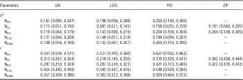
Table 3 shows the estimates of mean and quantiles (0.025, 0.975) of the posterior distribution of the heritability and repeatability for the traits and models studied. Heritability estimated for these traits ranged from (LIN) 0.1669 to (POI) 0.2499 for NOV; (LOG) 0.0813 to (ZIP) 0.1809 for NGI; (LOG) 0.1189 to (ZIP) 0.2036 for NDG; (LIN) 0.1306 to (POI) 0.1943 for NCLV and (LIN) 0.1028 to (POI) 0.2027 for NEMB. Genetic effects varied much more when considering the oocyte production traits (NOV, NGI, NDG) than for the embryo production traits (NCLV and NEMB).
Estimates of mean and quantiles (0.025, 0.975) of the posterior distribution of the heritability (h 2) and repeatability (r) for the traits and models studied

LIN=linear model (untransformed variable); LOG=linear model (transformed variable); POI=Poisson model; ZIP=zero-inflated Poisson model.
In summary, LIN models yielded the lowest heritability estimates for the majority of traits. POI models captured the higher proportions of additive genetic effects, yielding the highest heritability values for all traits, except for NGI, which ZIP model provided the highest heritability value. NGI and NDG, traits that exhibited the highest frequency of zeros in the data, presented the lower heritability estimates when evaluated under LIN models. Especially for the NGI, LOG model presented an impaired capacity of detecting additive genetic effects.
Repeatability showed wide variation between models (Table 3). POI models detected higher proportions of permanent environment effects, except for zero-inflated traits (NGI and NDG), where ZIP models captured higher proportions, yielding higher repeatability coefficient estimates.
Model comparison and predictive ability
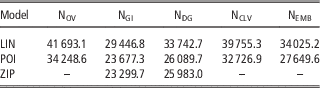
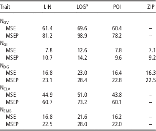
Table 4 presents the DIC values for all traits. Overall, DIC values were higher when considering LIN models. For NOV, NCLV and NEMB the lowest DIC values were obtained by POI models, and for NGI and NDG, DIC values for ZIP models were even lower. Mean squared error and mean squared error of prediction (MSEP) for the trait-model combinations analyzed in the present study are presented in Table 5. Considering the predictive ability of models, the standard POI models with residual term showed a pronounced superiority of over LIN, LOG models on fitting in vitro embryo production data, showing much lower MSE and MSEP values, and therefore, the least amount of bias. However, for the traits that presented an excessive number of zeros (NGI and NDG), one more time, ZIP models slightly outperformed POI models. LOG models showed higher MSE through all variables. Overall, MSEP values were in accordance to MSE for all trait-model combinations.
Estimated deviance information criterion for linear model (untransformed variable) (LIN), Poisson model (POI) and zero-inflated Poisson model (ZIP) models

LOG=linear model (transformed variable).
Mean squared error (MSE) and mean squared error of prediction (MSEP) between observed and fitted values for all trait-model combinations studied

LIN=linear model (untransformed variable); LOG=linear model (transformed variable); POI=Poisson model; ZIP=zero-inflated Poisson model.
aPredicted values were back transformed to observed scale.
Correlation between estimated breeding values
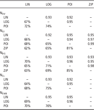
When considering all estimated breeding values, Spearman’s correlation coefficients had low variation between models for each variable (Table 6). These values varied from 0.92 (NOV – LIN and POI) to 0.99 (NGI – POI and ZIP). When considering the 10% higher estimated breeding values, the percentage of repeated animals for both models, NGI presented the lower values, from 0.62 (LIN and ZIP) to 0.81 (POI and ZIP), while NEMB had the highest values, varying from 0.69 (LOG and LIN) to 0.76 (POI and LOG). Considering mentioned similarities between top 10% estimated breeding value rankings, comparisons between LIN and ZIP (when applied) had the lowest percentage of repeated animals. Also, LIN models yielded the most uncorrelated rankings when comparing the 10% top individuals when compared with other models. In addition, POI and ZIP models resulted in very similar rankings for the 10% top breeding values, having 81% and 85% of repeated animals for NGI and NDG, respectively.
Spearman’s (rank) correlation coefficient between the estimated breeding values in the entire data set (above diagonal) and percentage of selected individuals in common considering the 10% higher estimated breeding values (below diagonal) from all trait-model combinations

LIN=linear model (untransformed variable); LOG=linear model (transformed variable); POI=Poisson model; ZIP=zero-inflated Poisson model.
Discussion
Gaussian mixed models are widely implemented in quantitative genetics and animal breeding, but their usage for modeling discrete traits is questionable (Gianola and Rosa, Reference Gianola and Rosa2015) if not under an adequate variable transformation. However, assuming discrete distributions can be an interesting approach rather to test robustness or to assess the bias generated by these transformations on animal breeding problems.
Variance components and ratios
Heritabilities estimates for in vitro embryo production traits are scarce in literature. Merton et al. (Reference Merton, Ask, Oonkundi, Mullaart, Collenbrander and Nielen2009), while studying genetic components involved on in vitro embryo production performance in Holstein cattle using sire models, reported heritabilities of 0.25, 0.19 and 0.16 for the number of cumulus–oocyte complexes, number of cleaved embryos and the number of viable embryos, respectively. Perez et al. (Reference Perez, Peixoto, Bruneli, Ramos and Balieiro2016), using a data set similar to this one of the present study, estimated genetic parameters for in vitro embryo production traits in Guzerá cattle using logarithmic transformation (log e X+1) of the evaluated variables. Heritability estimates varied from 0.08 and 0.19 for oocyte/embryo count traits. Both mentioned studies used restricted maximum likelihood (REML) method for variance component estimation. Ranges of heritability estimated in the present study were, in general, lower than reported by Merton et al. (Reference Merton, Ask, Oonkundi, Mullaart, Collenbrander and Nielen2009). A possible reason for the difference of heritability estimates between similar traits is that NOV (analyzed in this study) did not include grade IV oocytes as viable, an approach not followed by Merton et al. (Reference Merton, Ask, Oonkundi, Mullaart, Collenbrander and Nielen2009). However, those differences may also be associated with different selection criteria applied over Guzerá and Holstein populations, as well as the natural selection throughout the history of both breeds.
We believe that studies accounting for the genetic variation on in vivo embryo production may indirectly support inference on traits related to the embryos on in vitro process. Peixoto et al. (Reference Peixoto, Pereira, Bergmann, Penna and Fonseca2004) worked with Nellore cattle donors, also under superovulation, and estimated heritability of 0.20 for the number of transferable embryos. König et al. (Reference König, Bosselmann, Von Borstel and Simianer2007) have estimated heritability of 0.096 for the number of transferable embryos collected after superovulation in Holstein donors. This trait can be interpreted as similar to NEMB as it refers to the oocyte ability to be fertilized under artificial reproduction processes. In the present study, heritability estimates for the number of embryos produced in IVF (NEMB) ranged from 0.11 (LIN) to 0.20 (POI). Results suggest that even with the high environmental pressure suffered by those traits, there is an important genetic component affecting in vitro embryo production.
For our knowledge, this study was the first to report how permanent environment effects in vitro embryo production traits may vary under different modeling strategies. As for the genetic variance component, when comparing generalized linear mixed models and linear mixed models, inferences must be grounded on variance component ratios. The high repeatability presented for NOV (from 0.54 to 0.63) indicate that selection based on records from earlier ages of the cow may yield good response for lifetime oocyte production in Guzerá donors.
Repeatability estimated by LIN and LOG models were similar when compared within traits but were higher when under POI and ZIP models. Peñagaricano et al. (Reference Peñagaricano, Urioste, Naya, De Los Campos and Gianola2010) performed a genetic analysis of the number of black spots in Corriedale sheep and observed that POI models captured more variation from permanent environment effect when compared with linear models. Repeatability estimates by these authors were 0.35 and 0.75 to, respectively, linear and POI models for the same trait. The same behavior has been reported by Abdolahi-Arpanahi et al. (Reference Abdolahi-Arpanahi, Peñagaricano, Aliloo, Ghiasi and Urioste2013) when modeling the number of inseminations to conception on Iranian Holstein cows, and by Pérez-Cabal et al. (Reference Pérez-Cabal, De Los Campos, Vazquez, Gianola, Rosa, Weigel and Alenda2009) working with clinical mastitis counts on Spanish Holstein cows.
Although lower than genetic and permanent environment variances, sire (used in IVF) variance showed considerable values for NCLV and NEMB, varying from 2% to 14%, depending on the model applied. POI models have captured the highest IVF bull effects over NCLV and NEMB. Working with a smaller data set from the same population, Perez et al. (Reference Perez, Peixoto, Bruneli, Ramos and Balieiro2016) reported 1.1% and 4.8% of the total variation explained by the service sire (father of the embryos) effect analyzing data after variable transformation by REML, which are in accordance to the values estimated for the present study (1.96% for NCLV and 3.56% for NEMB) under LOG models.
General model comparison
Considering that the size of the data set used in the present study was relatively small, future applications of Bayesian Poisson and ZIP models in the routine of animal breeding programs (big data sets) could significantly increase the time for analysis completion. However, as the analyzes were performed using an interpreted programming language (R Development Core Team, 2016), the execution timings obtained must be interpreted with care. Further implementations of POI/ZIP Bayesian models using compiled languages such as C++ and Fortran could consistently reduce execution timings.
Deviance information criterion values were considered to compare LIN, POI and ZIP models. For NOV, NCLV and NEMB, POI models exhibited the lowest DIC values, which indicate that the count model outperformed Gaussian models when modeling these traits. For NGI and NDG, which had considerable number of zeroes, ZIP model had the lowest values of DIC. Differences on DIC (i.e. DICPOI – DICZIP) were 377 and 107 for NGI and NDG, respectively. These differences were lower than DIC values between LIN and POI models. Despite small differences to POI models, it indicates ZIP models better modeled that overdispersion caused by the excessive number of zeroes. The superiority of zero-inflated versions of standard hierarchical models in animal breeding was also reported by Varona and Sørensen (Reference Varona and Sørensen2010), while modeling pig mortality traits.
Goodness of fit and predictive ability upon cross-validation
Mean predicted residual sums of squares (MSEP) and obtained upon threefold cross-validation are shown in Table 5. Overall, POI models exhibited the lower MSE values for the ‘non-zero-inflated’ studied traits, while ZIP models had slightly lower MSE for the zero-inflated traits (NGI and NDG) indicating that it better fitted the data in this specific situation. Some authors have reported the same behavior for the standard POI model (Naya et al., Reference Naya, Urioste, Chang, Rodrigues-Motta, Kremer and Gianola2008; Peñagaricano et al., Reference Peñagaricano, Urioste, Naya, De Los Campos and Gianola2010; Vaquez et al., Reference Vazquez, Gianola, Bates, Weigel and Heringstad2012; Ayres et al., Reference Ayres, Pereira, Boligon, Silva, Schenkel, Roso and Albuquerque2013), while others have reported lower goodness of fit for the POI model when compared with linear models (Vazquez et al., Reference Vazquez, Pérez-Cabal, Heringstad, Rodrigues-Motta, Rosa, Gianola and Weigel2009a; Abdolahi-Arpanahi et al., Reference Abdolahi-Arpanahi, Peñagaricano, Aliloo, Ghiasi and Urioste2013; Ventura et al., Reference Ventura, Silva, Varona, Figueiredo, Costa, Silva, Ventura and Lopes2015). In general, we believe that traits in which distribution show more variation on the tail seem to get better fit by POI models, while traits that do not exhibit consistent variation on the tails show a slightly better (although often very similar) goodness of fit for the linear models. LOG models showed the higher values of MSE and, therefore, the lowest goodness of fit for the traits related to in vitro embryo production in Guzerá cattle. Thus, this last approach is not indicated for modeling these count traits. Ayres et al. (Reference Ayres, Pereira, Boligon, Silva, Schenkel, Roso and Albuquerque2013) also noticed similar results when studying tick counts in Hereford×Nellore crossed animals. Predictive ability in cross-validation studies indicates how precise a model is when predicting future phenotypic values. Overall, POI models outperformed all other (LIN, LOG) for NOV, NCLV and NEMB on threefold cross-validation. Specifically, to NGI and NDG, ZIP models exhibited lower values of MSE and MSEP, which reinforce that variables with excess of ‘zero’ (0) were better modeled by ZIP models. As observed for the MSE values, LOG models performed the worse on predictive ability (MSEP) when compared with the other models proposed. These results indicate the robustness of the POI models under Bayesian methods and the clear limitations of direct variable transformation on in vitro embryo production genetic analysis in Guzerá cattle.
Correlations between breeding values and estimated breeding values ranking similarities
As decisions on animal breeding are mainly made over animal’s genetic merit rankings, association between breeding values estimated from different models is an important question to be considered in animal breeding programs.
Spearman’s correlation coefficients between additive genetic effects estimated for the models fitted to each trait showed lower variation, and consequently, animals were similarly ranked independent of the modeling strategy adopted (Table 6). Likewise, Vazquez et al. (Reference Vazquez, Pérez-Cabal, Heringstad, Rodrigues-Motta, Rosa, Gianola and Weigel2009a) and Ayres et al. (Reference Ayres, Pereira, Boligon, Silva, Schenkel, Roso and Albuquerque2013) have reported correlations from 0.89 to 0.94 between breeding values estimated under Gaussian and POI models. When comparing POI and Gaussian models for traits exhibiting much less variation (number of spots), Peñagaricano et al. (Reference Peñagaricano, Urioste, Naya, De Los Campos and Gianola2010) reported a value of 0.76 for the Spearman rank correlation coefficient when comparing POI and Gaussian models.
The percentage of animals repeated on the top 10% of estimated breeding values between models within each trait show moderate ranking similarities ranging from 62% to 85% and, therefore, indicate that although the linear correlation for (all estimated) EBVs between models were high, the top genetic merit individuals tend to suffer more ranking variation. This reinforces the usage of standard POI and ZIP models over Gaussian models when analyzing count traits related to in vitro embryo production.
Conclusions
In vitro embryo production traits have low and medium heritability. Repeatability estimates were, in general, medium to high. Poisson and ZIP models captured higher genetic and permanent environment effects among all tested models. POI models fitted better than LIN and LOG models. When applied, ZIP models overcame POI models for traits with excessive number of zeroes (NGI and NDG). Correlation between estimated breeding values was high independent of the model. Results for the number of repeated animals on the top 10% genetic merit suggest the importance of choosing POI and ZIP models over Gaussian models for a more accurate selection for count traits. Logarithmic transformation is not indicated for modeling in vitro embryo production traits on Guzerá cattle.
Acknowledgments
The authors thank Fundação de Apoio à Pesquisa de Minas Gerais (Fapemig) and Coordenação Nacional do Pessoal de Nível Superior (CNPq) for the financial support provided for this study. We also would like to thank Cenatte Embriões for provisioning the data used for this study.
Supplementary material
To view supplementary material for this article, please visit https://doi.org/10.1017/S175173111700012X