1 Introduction
Bent pipes are ubiquitous in both man-made devices and biological systems. Their application in industry ranges from junctions between sections of straight pipes, to exhaust tubes and heat exchangers, just to name a few examples. The reasons for their vast employment are, amongst others, their enhanced cross-sectional mixing and improved mass and heat transfer coefficients, which make them an attractive alternative to traditional mechanical systems (for a comprehensive review see Vashisth, Kumar & Nigam Reference Vashisth, Kumar and Nigam2008). Even biological organisms contain curved ‘pipes’ which constitute, for instance, respiratory and vascular systems. In these cases the interest lies in understanding the influence that the vortical structures, formed due to the secondary flow, have on the circulation of fluid (Bulusu, Hussain & Plesniak Reference Bulusu, Hussain and Plesniak2014). In addition, the flow inside bent pipes is important for the research on hydrodynamic stability and transition to turbulence. In fact, the geometry of bent pipes exhibits only a few differences with respect to that of the most canonical and studied wall-bounded flow case of the past century, i.e. the straight pipe, but little is known about the onset of turbulence in curved pipes.
The earliest studies on bent pipes date as far back as to the nineteenth century (Boussinesq Reference Boussinesq1868). At the beginning of the past century, Eustice (Reference Eustice1910) measured a reduction of fluid flux and was able to correlate it directly with the curvature of the pipe. He later demonstrated, in a series of experiments, the existence of secondary flow by injecting coloured filaments of dye into water flowing through coiled pipes. Dean (Reference Dean1927) analysed the structure of the secondary motion by solving an approximate form of the Navier–Stokes equations valid in the limit of vanishing curvature. By considering a toroidal pipe he deduced that the flow could be described by a single dimensionless parameter which accounted for both Reynolds number and curvature. Employing this approximation he qualitatively confirmed the results of Eustice and showed that the secondary flow is composed of two counter-rotating vortices located mirror-symmetrically with respect to the equatorial plane of the torus. The non-dimensional number and the two vortices were later given Dean’s name in his honour. It is worth noting that, since Dean’s original work, the Dean number has been given several different definitions (see Berger, Talbot & Yao Reference Berger, Talbot and Yao1983, p. 471). In the present work, for the short part where it is needed, the following definition is employed:
 $De=\mathit{Re}\sqrt{{\it\delta}}$
, as strongly suggested by Berger et al. (Reference Berger, Talbot and Yao1983), and employed in the vast majority of follow-up studies. Here, and in the following,
 $\mathit{Re}$
is the Reynolds number, based on the diameter of the pipe, bulk velocity and fluid kinematic viscosity, i.e.
 $\mathit{Re}=2R_{p}U_{b}/{\it\nu}$
, while the curvature of the torus is the ratio between pipe and torus radii, i.e.
 ${\it\delta}=R_{p}/R_{t}$
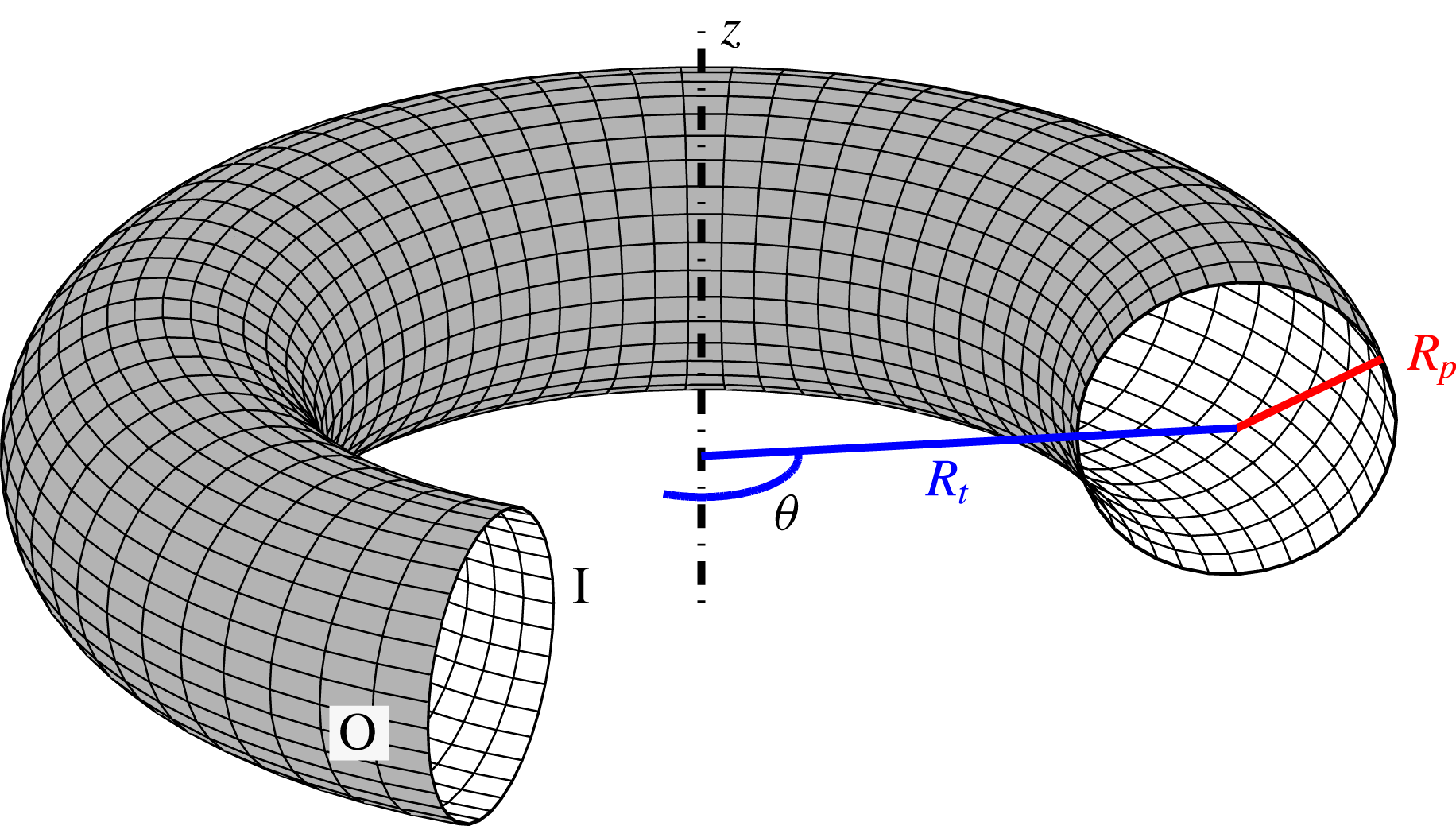
, cf. figure 1. Following Dean, other authors analysed the behaviour of the flow in a toroidal pipe (see e.g. McConalogue & Srivastava Reference McConalogue and Srivastava1968; Van Dyke Reference Van Dyke1978; Dennis Reference Dennis1980), further characterising the steady-state solution in the low-curvature limit (comprehensive reviews can be found in Berger et al. (Reference Berger, Talbot and Yao1983) and Ito (Reference Ito1987)).
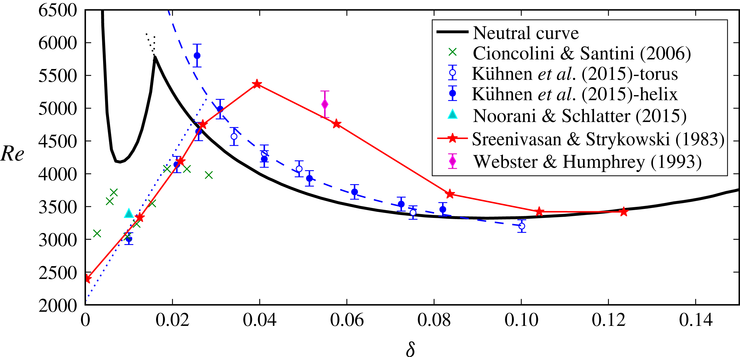
Experimental works were initially aimed at characterising the consequences of the secondary flow in mildly bent pipes. In particular, measurements of frictional resistance for turbulent flow in curved tubes were presented by a number of authors (see, most prominently, Ito (Reference Ito1959) and more recently Cioncolini & Santini (Reference Cioncolini and Santini2006)). The first studies that touch upon the topic of transition are those by Taylor (Reference Taylor1929) and White (Reference White1929), conducted in helical pipes and devoted to frictional resistance measurements. Later, Sreenivasan & Strykowski (Reference Sreenivasan and Strykowski1983) conducted similar experiments with a helical pipe at low curvatures. The authors employed both dye streaks and hot-wire anemometry to obtain insight into the transitional flow. Although, as stated in the paper, their investigation was at a preliminary stage, these authors were, to the best of our knowledge, the first to observe the subcritical transition boundary for low curvatures. A more detailed analysis is provided by Webster & Humphrey (Reference Webster and Humphrey1993, Reference Webster and Humphrey1997) who examined the flow inside a helical pipe with curvature
 ${\it\delta}=0.055$
. They observed a transition from steady to periodic flow occurring for a Reynolds number
 $\mathit{Re}=5060$
. The periodic regime revealed the presence of a travelling wave on top of the Dean vortices.
Sketch of the torus showing the definition of the curvature
 ${\it\delta}=R_{p}/R_{t}$
. The ‘I’ and ‘O’ labels indicate the inner, respectively outer, portions of the pipe;
 $z$
is the axis of the torus. The pipe is cut for illustrative purposes only.

Without the small curvature approximation, Hüttl & Friedrich (Reference Hüttl and Friedrich2001) presented direct numerical simulations (DNS) of the flow inside portions of toroidal and helical pipes with curvatures of 0.01 and 0.1. The computations were performed with a finite volume code and periodic boundary conditions were applied at the end sections. Their paper focuses mainly on the reduction of turbulence intensity due to the curvature, and does not present quantitative comparisons with the experiments by Sreenivasan & Strykowski (Reference Sreenivasan and Strykowski1983), Webster & Humphrey (Reference Webster and Humphrey1997), which are in a similar range of Reynolds numbers. Noorani, El Khoury & Schlatter (Reference Noorani, El Khoury and Schlatter2013) reproduced the results for low curvature, confirming their validity, and provided the first turbulence budgets for bent pipes.
Di Piazza & Ciofalo (Reference Di Piazza and Ciofalo2011) simulated the flow in the entirety of a torus, with another finite volume code. This is, to the best of our knowledge, the first work aimed at understanding the cause of instability of this flow. Two values of curvature were investigated (0.1 and 0.3) and both showed a transition from stationary to periodic, quasi-periodic and then chaotic flow. However, as indicated by Kühnen et al. (Reference Kühnen, Braunshier, Schwegel, Kuhlmann and Hof2015) and as will be shown herein, these results should be considered inaccurate, with the exception of the symmetry characteristics observed in the flow. The only experiments employing toroidal pipes are those by Kühnen et al. (Reference Kühnen, Holzner, Hof and Kuhlmann2014, Reference Kühnen, Braunshier, Schwegel, Kuhlmann and Hof2015). These authors sacrificed the
 $2{\rm\pi}$
(streamwise) periodicity and the mirror symmetry of the system by introducing a steel sphere in the tube to drive the fluid. This resulted, as mentioned in their first paper, in a non-symmetric mean flow and the absence of any considerations on the symmetry characteristics of the periodic flow. Their results for
 $0.028<{\it\delta}<0.1$
confirmed the findings of Webster & Humphrey (Reference Webster and Humphrey1993), i.e. that the first instability leads the flow to a periodic regime, while for
 ${\it\delta}<0.028$
subcritical transition was observed, as in Sreenivasan & Strykowski (Reference Sreenivasan and Strykowski1983). With the exception of these papers focusing on the low-curvature limit, no complete stability analysis for this flow is available in the literature.
The present analysis is conducted in a toroidal pipe in order to isolate the effect of the curvature from that of the torsion of a helix as well as that of inflow and outflow sections. A straight pipe is characterised by a central symmetry through its axis. Bending the pipe breaks this symmetry and leaves the system with a discrete reflectional symmetry about the equatorial plane of the torus. Bending the pipe further into an helical one breaks this symmetry as well. Thus, although moderate curvature or torsion may not significantly affect global quantities, such as the pressure drop between inlet and outlet, these deformations structurally modify the geometry of the flow. The paper continues with a description of the approach employed, presented in § 2, while the base flow and its characteristics are described in § 3. Section 4 presents the results of the linear analysis which are then compared with the nonlinear behaviour in § 5 and finally discussed and compared with the literature in § 6.
2 Numerical set-up
The fluid inside the torus is considered viscous and incompressible and therefore satisfies the incompressible Navier–Stokes equations
 $$\begin{eqnarray}\displaystyle & \displaystyle {\displaystyle \frac{\partial \boldsymbol{u}}{\partial t}}+(\boldsymbol{u}\boldsymbol{\cdot }\boldsymbol{{\rm\nabla}})\boldsymbol{u}-{\displaystyle \frac{1}{\mathit{Re}}}{\rm\nabla}^{2}\boldsymbol{u}+\boldsymbol{{\rm\nabla}}\!p=\boldsymbol{f}, & \displaystyle\end{eqnarray}$$
 $$\begin{eqnarray}\displaystyle & \boldsymbol{{\rm\nabla}}\!\boldsymbol{\cdot }\boldsymbol{u}=0, & \displaystyle\end{eqnarray}$$
 $\boldsymbol{u}(\boldsymbol{r},t)$
is the velocity vector, with components
 $\boldsymbol{u}=(u_{r},u_{{\it\theta}},u_{z})$
in cylindrical coordinates,
 $p$
is the (dimensionless) pressure which has been rescaled by dividing by the Reynolds number
 $\mathit{Re}$
and
 $\boldsymbol{f}$
represents a volume force. The Reynolds number is based on the diameter of the pipe and the bulk velocity, i.e.
 $\mathit{Re}=2R_{p}U_{b}/{\it\nu}$
.
The steady solutions and the stability results presented in this paper have been computed with PaStA, an in-house developed software package. PaStA is a Fortran90 code, written in primitive variables and based on the finite element method (FEM) employing triangular
 $\mathbb{P}_{2}{-}\mathbb{P}_{1}$
elements; it relies on the MUMPS library (Amestoy, Duff & L’Excellent Reference Amestoy, Duff and L’Excellent2000) for the solution of linear systems (for details, see Canton Reference Canton2013). The time-dependent simulations, on the other hand, have been performed by means of the spectral element code nek5000 (Fischer, Lottes & Kerkemeier Reference Fischer, Lottes and Kerkemeier2008). Convergence and accuracy tests have been performed to a more than satisfactory degree by comparing results to reference ones, whenever possible, or by comparing the two codes when results were new. These tests are omitted from this article for conciseness; some can be found in Canton (Reference Canton2013), Noorani et al. (Reference Noorani, El Khoury and Schlatter2013). However, we demonstrate excellent agreement between the linear analysis and the nonlinear DNS performed with two different codes, employing two different methods, in § 5.
The stability of the flow is studied in a classical framework: as a first step, a fixed point for the system, i.e. a steady solution to (2.1), is computed with the nonlinear solver, which employs Newton’s method. Subsequently, its stability properties are investigated by linearising the system about this steady state, and computing the leading eigenvalues of the linearised Navier–Stokes operator,
 $\mathscr{L}$
. By employing an expansion in normal modes, the perturbation fields are defined as
 $$\begin{eqnarray}\boldsymbol{u}^{\prime }(r,{\it\theta},z,t)=\hat{\boldsymbol{u}}(r,z)\exp \text{i}(k{\it\theta}-{\it\omega}t),\quad p^{\prime }(r,{\it\theta},z,t)=\hat{p}(r,z)\exp \text{i}(k{\it\theta}-{\it\omega}t),\end{eqnarray}$$
where
 $k\in \mathbb{R}$
is the streamwise wavenumber,
 ${\it\omega}={\it\omega}_{\mathit{r}}+\text{i}{\it\omega}_{\mathit{i}}\in \mathbb{C}$
is the eigenvalue and
 $\hat{\boldsymbol{u}}\in [\mathbb{C}]_{2}^{3}$
and
 $\hat{p}\in [\mathbb{C}]_{2}$
form the eigenfunction
 $\hat{\boldsymbol{x}}=(\hat{\boldsymbol{u}},\hat{p})$
. Note that here, and in the following, the symbols
 $[\mathbb{A}]_{d}^{c}$
are used to denote a
 $c$
-dimensional vector space
 $\mathbb{A}$
in a
 $d$
-dimensional physical space; it is clear that when
 $c$
is omitted
 $\mathbb{A}$
represents a scalar space. Although
 $k$
is in principle a real number, the
 $2{\rm\pi}$
-periodicity of the torus restricts it to
 $\mathbb{Z}$
.
The linearised Navier–Stokes equations, discretised via the finite element method, are thus reduced to a generalised eigenvalue problem of the form
 $$\begin{eqnarray}\text{i}{\it\omega}\unicode[STIX]{x1D648}\hat{\boldsymbol{x}}=\unicode[STIX]{x1D647}_{k}\hat{\boldsymbol{x}},\end{eqnarray}$$
where
 $\hat{\boldsymbol{x}}$
is the discretised eigenvector,
 $\unicode[STIX]{x1D648}\in \mathbb{R}^{\mathit{dof}\times \mathit{dof}}$
is the (singular) generalised mass matrix,
 $\unicode[STIX]{x1D647}_{k}\in \mathbb{C}^{\mathit{dof}\times \mathit{dof}}$
represents the discretisation of the linearised Navier–Stokes operator
 $\mathscr{L}$
, parametrised by the streamwise wavenumber
 $k$
. Finally, ‘
 $\text{dof}$
’ is a shorthand for the total number of degrees of freedom, the number of unknowns of the problem, which accounts for both velocity and pressure, i.e.
 $\text{dof}=c(\mathbb{P}_{2}~\text{nodes})+(\mathbb{P}_{1}~\text{nodes})$
. The eigensolutions are computed to machine precision through an interface to the ARPACK library (Lehoucq, Sorensen & Yang Reference Lehoucq, Sorensen and Yang1998), where the shift-invert spectral transformation is used to accelerate convergence to the desired portion of the spectrum. The eigenmodes determine whether the fixed point is stable or not, to locate the non-hyperbolic points of the system and, in the event of a bifurcation point, to determine the type of the bifurcation.
Once a bifurcation is identified and its type determined, its neutral curve can be traced in parameter space, separating the stable and unstable regions. In order to track a bifurcation, an augmented set of equations describing the system at the bifurcation point, i.e. where the critical eigenvalue has zero growth rate, needs to be solved. Equation (2.4a–c ) presents this system in the case of a Hopf bifurcation, which is the type of bifurcation encountered by this flow,
 $$\begin{eqnarray}\displaystyle & \unicode[STIX]{x1D649}\boldsymbol{x}=0, & \displaystyle\end{eqnarray}$$
 $$\begin{eqnarray}\displaystyle & \text{i}{\it\omega}_{\mathit{r}}\unicode[STIX]{x1D648}\hat{\boldsymbol{x}}=\unicode[STIX]{x1D647}_{k}\hat{\boldsymbol{x}}, & \displaystyle\end{eqnarray}$$
 $$\begin{eqnarray}\displaystyle & {\bf\phi}\boldsymbol{\cdot }\hat{\boldsymbol{x}}=1, & \displaystyle\end{eqnarray}$$
 $\unicode[STIX]{x1D649}=\unicode[STIX]{x1D649}(\mathit{Re},{\it\delta},\boldsymbol{x})\in \mathbb{R}^{\mathit{dof}\times \mathit{dof}}$
,
 $\unicode[STIX]{x1D648}=\unicode[STIX]{x1D648}({\it\delta})\in \mathbb{R}^{\mathit{dof}\times \mathit{dof}}$
, and
 $\unicode[STIX]{x1D647}_{k}=\unicode[STIX]{x1D647}_{k}(\mathit{Re},{\it\delta},\boldsymbol{x})\in \mathbb{C}^{\mathit{dof}\times \mathit{dof}}$
. The unknowns for this system are: the base flow, i.e. the steady solution to (2.1), comprising both velocity and pressure,
 $\boldsymbol{x}=(\boldsymbol{u},\boldsymbol{p})\in \mathbb{R}^{\mathit{dof}}$
; the frequency of the critical eigenmode,
 ${\it\omega}_{\mathit{r}}\in \mathbb{R}$
; and the corresponding eigenvector,
 $\hat{\boldsymbol{x}}=(\hat{\boldsymbol{u}},\hat{\boldsymbol{p}})\in \mathbb{C}^{\mathit{dof}}$
. The pair
 $\mathit{Re},{\it\delta}\in \mathbb{R}$
can act as unknown/parameter or, vice versa, as parameter/unknown, where one is fixed while the other is obtained as part of the solution. Equation (2.4a
) is a real equation which determines the base flow:
 $\unicode[STIX]{x1D649}$
constitutes the discretised steady-state Navier–Stokes equations, i.e. it is shorthand for a steady solution to (2.1). This is the nonlinear equation that is solved when computing a steady state, regardless of whether it is on the neutral curve or not. Equation (2.4b
) is a complex equation which represents the eigenvalue problem (2.3) in the particular case where a pair of complex conjugate eigenvalues has zero growth rate. This equation forces the solution of the system to be on the neutral curve. Equation (2.4c
) is a complex equation as well, it fixes the phase and amplitude of the eigenvector. The constant vector
 ${\bf\phi}$
is chosen as the real part of the initial guess for
 $\hat{\boldsymbol{x}}$
, so that this linear equation mimics an
 $L^{2}$
norm.
Newton’s method is employed for this large nonlinear system as well. In contrast with the standard procedure, though, the full Jacobian matrix for (2.4a–c
) is not assembled, as its size would be
 $3\text{dof}+2\times 3\text{dof}+2$
, and its sparsity pattern would need to be created. Instead, a block Gauss factorisation and linear algebra are used to split the resulting system into five
 $\text{dof}\times \text{dof}$
linear systems, two real and three complex. In addition to reducing memory requirements, these systems have matrices with the same sparsity pattern as those already used for the solution of the steady state and the eigenvalue problem. The method is similar to those presented in Salinger et al. (Reference Salinger, Bou Rabee, Pawlowski, Wilkes, Borroughs, Lehoucq and Romero2002), but here the Jacobian matrix for the steady state is not equivalent to the linearised Navier–Stokes operator
 $\unicode[STIX]{x1D647}_{k}$
. The tolerance for the iterative solution of (2.4a–c
) was chosen as to have an uncertainty of
 $\mathit{Re}$
on the neutral curve of
 $\pm 10^{-4}\,\%$
on a mesh with 98 870 elements, corresponding to
 $\text{dof}=646\,327$
.
3 Base flow
The fluid, flowing inside the pipe at constant mass rate, is maintained in motion by a volume force aligned with the centreline of the torus and defined as
 $\boldsymbol{f}=\boldsymbol{e}_{{\it\theta}}F/r$
. Here
 $F$
is a scalar constant and
 $r$
represents the distance from the axis of the torus. The inverse proportionality to
 $r$
is required so that the integral of
 $\boldsymbol{f}$
along the curvilinear coordinate
 $\boldsymbol{s}=r{\bf\theta}$
is independent of
 $r$
, i.e.
 $\int \boldsymbol{f}\boldsymbol{\cdot }\text{d}\boldsymbol{s}=\int (F/r)r\boldsymbol{e}_{{\it\theta}}\boldsymbol{\cdot }\text{d}{\bf\theta}=F({\it\theta}-{\it\theta}_{0})~\forall r$
. This property confers on
 $\boldsymbol{f}$
a role similar to that of the pressure in straight pipes (or channels) and it ensures continuity with a straight pipe for a torus in the limit of vanishing curvature. In fact, when
 ${\it\delta}\rightarrow 0$
,
 $r\rightarrow \infty$
on the section of the toroidal pipe, then
 $\boldsymbol{f}$
tends to a value which is uniform on the section of the pipe, as the pressure in a straight pipe.
The value of
 $F$
is determined via the secant method such as to have unitary bulk velocity. This cannot be done analytically since the relationship between
 $\boldsymbol{f}$
and
 $U_{b}$
is nonlinear and a priori unknown (see Ito Reference Ito1959).
The steady-state solution inherits both the rotational invariance and the mirror symmetry of the toroidal geometry and it is thus independent of
 ${\it\theta}$
and symmetric with respect to the equatorial plane of the torus. In addition to being evident from geometrical considerations, this has been confirmed by three-dimensional DNS performed for values of
 ${\it\delta}$
and
 $\mathit{Re}$
below criticality. The invariance with respect to
 ${\it\theta}$
allows the solutions to be computed on a two-dimensional section (retaining three velocity components), sensibly reducing the computational cost.
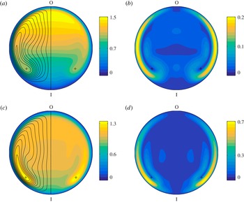
The base flow is characterised by the presence of two symmetric, counter-rotating Dean vortices. The side with the counterclockwise rotating vortex is visible in the contours of the streamfunction in figure 2(a,c), and the centres of the vortices are indicated with plus symbols. These vortices develop as a result of the centrifugal force arising from breaking the central symmetry characterising a straight pipe and are thus present at every Reynolds number and for any non-zero curvature. The question of a critical Dean number below which no recirculation occurs has been discussed in textbooks (see, for instance, Isachenko, Osipova & Sukomel Reference Isachenko, Osipova and Sukomel1974, p. 218). However, even for
 ${\it\delta}=10^{-11},~\mathit{Re}=1$
, corresponding to
 $De=\mathit{Re}\sqrt{{\it\delta}}\approx 3\times 10^{-6}$
, the vortices are present, albeit exhibiting low intensity; their presence for any non-zero curvature can also be shown analytically, cf. Dean (Reference Dean1927).
As can be observed in figure 2, which depicts two steady states for the same Dean number,
 $De=759$
, the curvature of the torus plays a primary role in determining the behaviour of the base flow, starting at least from
 ${\it\delta}=0.1$
. It greatly influences, among other features, the shape of the vortices, the position of the maximum velocity and the magnitude of the in-plane flow. An example can be observed in figure 2: the maximum of
 $u_{{\it\theta}}$
moves from the outer portion of the pipe for low curvature, figure 2(a), to the centre of the vortices, 2(c), for high curvature. Moreover, as discussed in the next section, the curvature is of primary importance for the characteristics of the first instability. We thus observe that the curvature of the pipe should be considered as a separate parameter with as much importance as the Reynolds number and that the Dean number alone is insufficient to describe the flow fully.
Steady state solutions for
 $De=759$
at different curvatures and Reynolds number: (a,b)
 ${\it\delta}=0.1$
,
 $\mathit{Re}=2400$
; (c,d)
 ${\it\delta}=0.9$
,
 $\mathit{Re}=800$
. Panels (a,c) depict the magnitude of the streamwise velocity component
 $u_{{\it\theta}}$
, and contours of the in-plane streamfunction
 ${\it\psi}$
for positive values; the plus symbols are located at the position of the maximum and minimum of
 ${\it\psi}$
. Panels (b,d) show the magnitude of the in-plane velocity. Quantities are normalised with the bulk velocity. The ‘I/O’ labels indicate the inner and outer portions of the pipe (see figure 1).

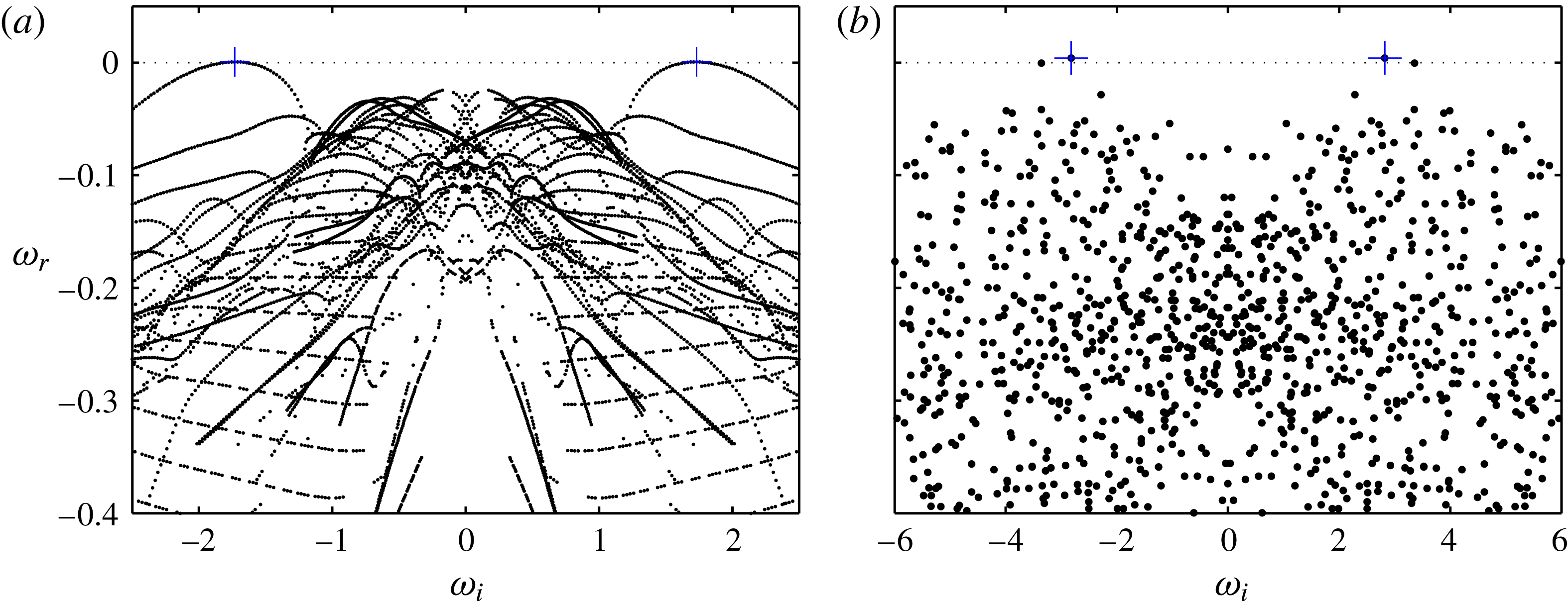
Eigenvalue spectra for the flow in a toroidal pipe. (a) Presents the spectrum for
 ${\it\delta}=0.01,\mathit{Re}=4300$
, corresponding to
 $De=430$
, while (b) is for
 ${\it\delta}=0.3,\mathit{Re}=3400$
, corresponding to
 $De\approx 1862$
. Both cases are moderately above criticality: the flow for
 ${\it\delta}=0.01$
becomes unstable for
 $\mathit{Re}>4257$
, while for
 ${\it\delta}=0.3$
 $\mathit{Re}_{\mathit{c}}=3379$
. The least-stable eigenvalues are highlighted with plus symbols. The wavenumber of the critical mode for
 ${\it\delta}=0.01$
is 74, while for
 ${\it\delta}=0.3$
 $k=7$
. The corresponding eigenvectors are depicted in figure 4. Note the striking difference in the structure of the spectra.

4 Stability analysis
The first step of the stability analysis was the computation of eigenvalue spectra on a coarse grid of points in parameter space,
 $({\it\delta},\mathit{Re})\in \left([0.005,1],[500,10^{4}]\right)$
. All curvatures in the grid revealed spectra with unstable eigenvalues for
 $\mathit{Re}<6\times 10^{3}$
. This result confirms the numerical observations by Di Piazza & Ciofalo (Reference Di Piazza and Ciofalo2011) as well as the experiments by Kühnen et al. (Reference Kühnen, Holzner, Hof and Kuhlmann2014, Reference Kühnen, Braunshier, Schwegel, Kuhlmann and Hof2015) and extends these studies, which are limited to the low curvature range. Most importantly, it proves that this flow is linearly unstable, in obvious contrast to the flow inside a straight pipe (see Schmid & Henningson (Reference Schmid and Henningson1994) and citations therein). Each spectrum in the grid exhibits a pair of complex conjugate eigenvalues as most unstable mode, indicating that the cause of the modal instability is a supercritical Hopf bifurcation. In fact, DNS confirm that the flow transitions from a steady state to a periodic state, characteristic of the stable limit cycle identified by this bifurcation. For a thorough discussion, see § 5.
Figure 3 presents, as examples, two supercritical eigenvalue spectra. These are for very low and moderate curvature,
 ${\it\delta}=0.01$
and
 $0.3$
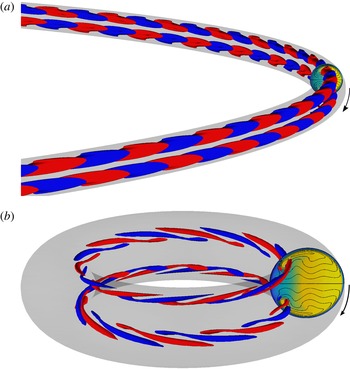
, respectively, and each has a complex conjugate eigenpair with positive growth rate. Although the instability is caused by a Hopf bifurcation for every curvature, the associated critical mode changes with the curvature of the pipe. This can be seen in figure 4, which shows the different spatial structure of the two critical modes presented in figure 3. The eigenmodes differ in their wavenumbers, temporal frequencies, spatial structure and symmetry properties. Figure 3 demonstrates a striking difference in the structure of the two spectra and the variation of the frequency of the critical mode. The set of spectra computed on the grid revealed a non-monotonic relationship between critical Reynolds number and curvature; even the variation of eigenmode characteristics, e.g. wavenumber, as a function of
 $({\it\delta},\mathit{Re})$
does not have a continuous trend. It is clear that a detailed analysis of the whole parameter space cannot be performed employing a coarse grid of points and interpolation between them.
Critical modes for (a)
 ${\it\delta}=0.01,~\mathit{Re}=4257$
and (b)
 ${\it\delta}=0.3$
,
 $\mathit{Re}=3379$
. Both modes are antisymmetric with respect to the equatorial plane of the torus. The wavenumbers are
 $k=74$
and
 $k=7$
respectively. Isocontours of opposite values of the streamwise velocity component are depicted in blue and red,
 $u_{{\it\theta}}=\pm 0.15$
in (a) and
 $u_{{\it\theta}}=\pm 2.2$
in (b). The vertical cuts depict the streamwise velocity and in-plane streamlines of the corresponding base flow. The fluid is flowing clockwise, as indicated by the arrows.

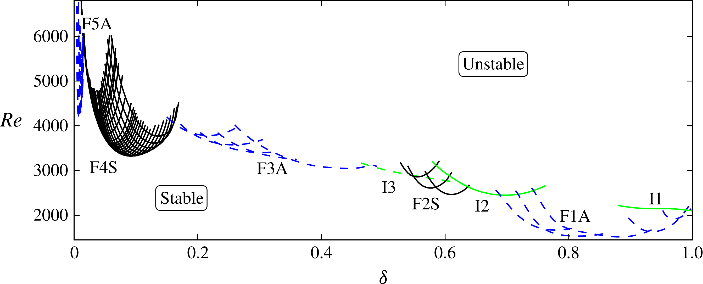
Employing the method described in § 2, the neutral curve of every critical mode has thus been traced in the parameter space as a function of curvature and Reynolds number. The result is a complex picture, depicted in figure 5. It presents five ‘families’ and three ‘isolated’ modes; their envelope constitutes the global neutral curve for the flow. All eigenmodes on this curve share the characteristic of representing a travelling wave, while all of the other properties are modified along the neutral curve. As anticipated in § 3, the curvature of the pipe plays a key role in determining the identity of the critical mode and its characteristics. The neutral curves cannot, in fact, be collapsed onto one another as a function of a single non-dimensional parameter, thereby confirming the need for two parameters (
 ${\it\delta}$
and
 $\mathit{Re}$
) to describe this flow.
A ‘family’ comprises eigenmodes that share common characteristics, while the eigenvalues designated as ‘isolated’ are those which contribute to the global neutral curve while being dissimilar to the modes belonging to the neighbouring neutral curves. In more detail, all modes belonging to a given family display the same spatial structure and symmetry properties, they have approximately equal phase speed and comparable wavelength. In addition, while the wavenumber does not vary monotonically along the envelope of neutral curves, it does so inside families. Furthermore, eigenvalues in the same family lie on the same branch. This is very clear for low curvatures: in figure 3(a) the two uppermost branches comprise eigenvalues belonging to the same family, the same holds for the two, nearly straight-line branches just below them, and so on. Possibly even more characteristic is the fact that the eigenmodes forming a family have neutral curves with a very similar trend
 $({\it\delta},\mathit{Re}({\it\delta}))$
. This can readily be observed in figure 5 where each neutral curve is purposely plotted beyond the envelope line to illustrate this feature.
Neutral curve in the
 ${\it\delta}{-}\mathit{Re}$
plane.
 ${\it\delta}\in [0.002,1]$
. Each line corresponds to the neutral curve of one mode. The neutral curve for the flow is formed by the envelope of the lines. Five families (black and blue) and three isolated modes (green) are marked by labels. Symmetric modes are indicated with continuous lines while antisymmetric modes are represented with dashed lines. Note that the curves are not interpolated, i.e. they are segments connecting computed solutions with
 ${\rm\Delta}{\it\delta}=\mathit{O}(10^{-3})$
. The uncertainty on the Reynolds number is
 $\pm 10^{-4}\,\%$
.

4.1 Description of the neutral curve
As previously mentioned, all neutral curves in figure 5 are traced beyond the point(s) where they leave the envelope for the sole purpose of illustrating their shape. For example, I1 is traced up to
 ${\it\delta}=0.9$
, but it stops being relevant for the instability boundary for
 ${\it\delta}<0.99$
, where the rightmost curve of F1A has lower
 $\mathit{Re}$
for the same curvatures.
Starting at unit curvature, the first contribution to the envelope of neutral curves is given by an isolated mode: the rightmost continuous line in figure 5, labelled I1. I1 represents a singular case for
 $0.99<{\it\delta}\leqslant 1$
: this is the only range of curvature values that has a critical mode with zero spatial wavenumber. This is, in fact, the only eigenmode with a stationary, symmetric structure pulsating at non-zero temporal frequency. This peculiar property is the effect of the singular geometrical condition approached by the pipe when
 ${\it\delta}$
nears unity, namely that of a ring torus with no ‘hole’: a horn torus. For
 ${\it\delta}\leqslant 0.99$
all critical modes are characterised by non-zero wavenumber. More specifically,
 $k$
increases monotonically as the curvature is lowered, but only between modes belonging to the same family; it has, however, discontinuities across different families.
A first family of eigenmodes (F1A in figure 5) appears at high curvature and relatively low Reynolds number. These modes are antisymmetric with respect to the equatorial plane of the torus and are characterised by
 $4\leqslant k\leqslant 8$
and particularly high phase speed (cf. figure 6). To the left of this family, for
 $0.64\leqslant {\it\delta}<0.69$
, a second isolated mode appears. This eigensolution has
 $k=6$
and has a symmetric spatial structure dissimilar to that of the two neighbouring families. In spite of these differences, this mode is also characterised by moderately high phase speed, somewhat similar to F1A.
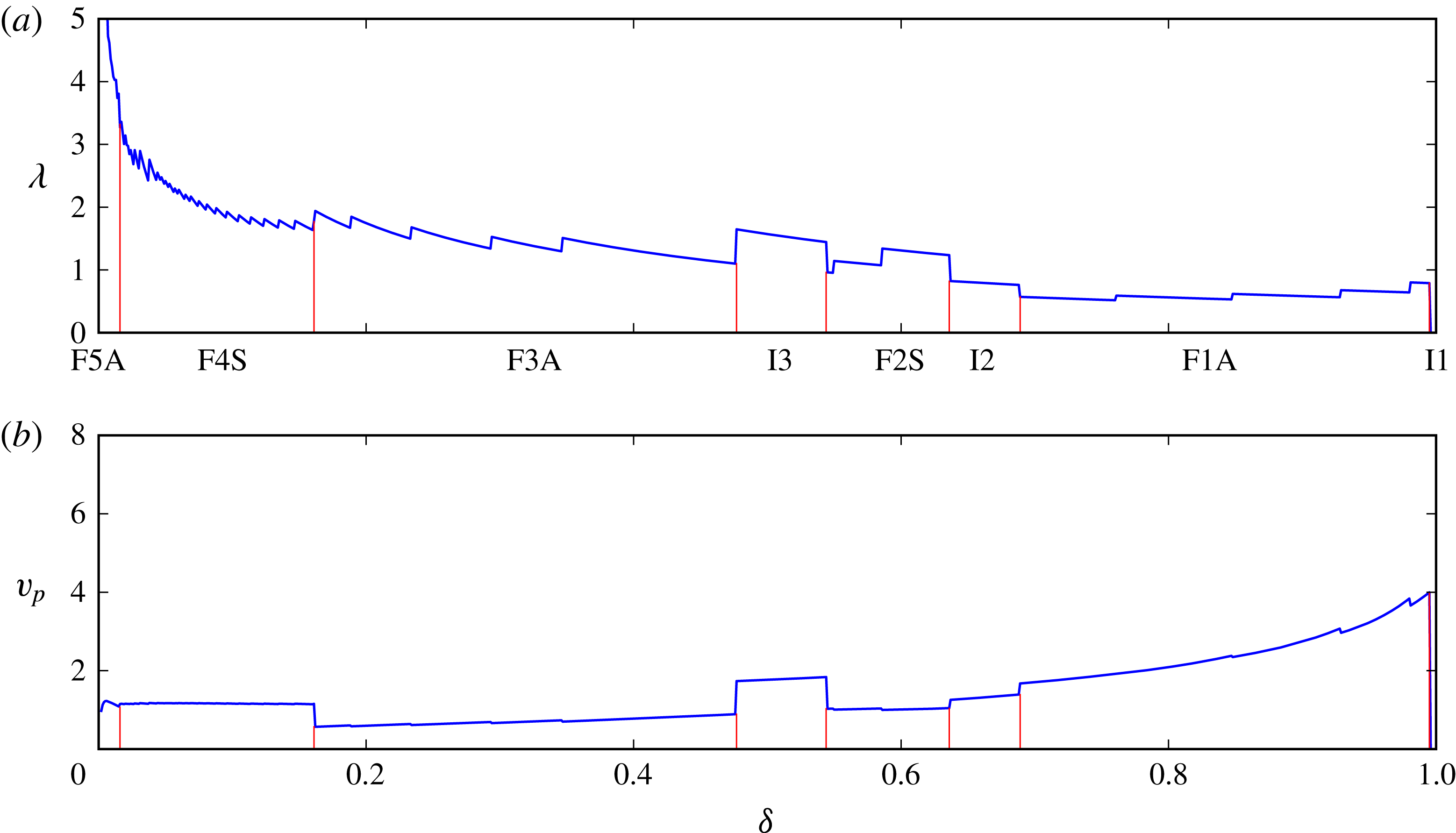
Envelopes of wavelength,
 ${\it\lambda}$
, and phase speed,
 $v_{p}$
, of the critical modes along the neutral curve. The boundaries between families and isolated modes are highlighted by thin vertical (red) lines. Both quantities are scaled with pipe diameter and bulk velocity.

The reason for the high phase speed of the modes at high curvature is probably due to a modification in the base flow. In fact, for
 ${\it\delta}>{\it\delta}_{s}\approx 0.6$
(the exact value depends on the Reynolds number) the maximum of streamwise velocity moves from the outer portion of the torus to the inner portion. The steady solutions depicted in figure 2 provide a clear example of this phenomenon. This shift causes a qualitative as well as quantitative change in the structure of the base flow which has, for
 ${\it\delta}>{\it\delta}_{s}$
, two symmetric maxima in the velocity field, located close to the cores of the Dean vortices. Both F1A and I2 comprise eigenvectors with a structure located very close to the Dean vortices. The oscillations that these modes produce in the flow are thus rapidly transported inside the pipe, giving rise to high-frequency fluctuations. At medium curvature, for
 $0.54\leqslant {\it\delta}<0.64$
, the instability is caused by a second family of symmetric modes, F2S. These modes, with
 $4\leqslant k\leqslant 6$
, are still located close to the Dean vortices but have moderate phase speed. The third isolated mode, on the other hand, is antisymmetric, has
 $k=4$
and high phase speed, and is critical for
 $0.48\leqslant {\it\delta}<0.54$
.
The third family, F3A, is responsible for the onset of the instability for
 $0.16<{\it\delta}<0.48$
. Even at this moderately low curvature the wavenumber associated with the eigenmodes grows slowly, ranging from 6 to 10 in this family of antisymmetric modes. Both frequency and phase speed decrease as the curvature is lowered, with the phase speed reaching its lowest value of 0.57 for
 ${\it\delta}=0.16$
. The Reynolds number, on the other hand, varies non-monotonically from 3112 to 4059. As an example, the critical mode for
 ${\it\delta}=0.3$
is depicted in figure 4(b), and the corresponding spectrum is in figure 3(b). Di Piazza & Ciofalo (Reference Di Piazza and Ciofalo2011) performed numerical simulations for
 ${\it\delta}=0.3$
that confirm the transition of the flow to a periodic regime exhibiting an antisymmetric, varicose travelling wave. However, their result indicates the stability of the steady state up to
 $\mathit{Re}\approx 4575$
, a value 35 % higher than ours, and the appearance of a travelling wave with
 $k=8$
, in contrast to the present
 $k=7$
.
Low curvatures are characterised by more organised eigenvalue spectra with isolated and ordered branches of modes (cf. figure 3). This feature is visible in figure 5 as well: the two leftmost families, F4S and F4A, are in fact more populated and continuous than the other ones. A further difference between low and high
 ${\it\delta}$
is that low-curvature eigenmodes show a spatial structure located towards the centre of the pipe, not close to the Dean vortices as observed for higher curvatures. This change in the structure of the modes, and the corresponding eigenspectra, is not surprising. In fact,
 ${\it\delta}$
is nearing its lower limit, and the torus is tending towards a straight pipe.
Family F4S has symmetric modes with
 $11\leqslant k\leqslant 60$
and is responsible for the instability for
 $0.016\leqslant {\it\delta}\leqslant 0.16$
. The eigenvalues belonging to this family can be observed in figure 3(a), where they form the branches just below the critical ones. This family was the one found by Kühnen et al. (Reference Kühnen, Braunshier, Schwegel, Kuhlmann and Hof2015), in the range
 $0.026\leqslant {\it\delta}\leqslant 0.1$
. It appears, from this experimental investigation, that F4S constitutes the instability boundary not only for toroidal pipes, but for low-pitch helical pipes as well. Di Piazza & Ciofalo (Reference Di Piazza and Ciofalo2011) presented a second set of data for
 ${\it\delta}=0.1$
. For this curvature, though, they found steady states up to
 $\mathit{Re}=5139$
, a value 54 % higher than the present
 $\mathit{Re}_{\mathit{c}}=3331$
. Moreover, they observed an hysteresis in the value of the Reynolds number separating the steady and periodic regimes. This observation is inconsistent with both the experimental results of Kühnen et al. (Reference Kühnen, Braunshier, Schwegel, Kuhlmann and Hof2015), and the numerical data presented here.
Our data presents one last family of modes below
 ${\it\delta}=0.016$
: F5A, constituted by antisymmetric eigenmodes. One of these eigenmodes is depicted in figure 4(a) and the eigenvalues belonging to F5A constitute the most unstable branches in figure 3(a). The wavenumber associated with these modes grows rapidly from
 $k=55$
to
 $k=95$
, where our neutral curves stop, but the computed eigenvalue spectra indicate that eigenvalues with
 $k>200$
belong to this family. As it will be shown in § 6, however, this range of curvatures has subcritical transition at lower Reynolds numbers.
Figure 6 shows the envelopes of wavelength,
 ${\it\lambda}=2{\rm\pi}R_{t}/k$
, and phase speed,
 $v_{p}={\it\omega}_{\mathit{r}}R_{t}/k$
, along the neutral curve, two characteristic quantities associated with the modes. Both quantities show the separation between families and isolated modes and illustrate the complexity of the neutral curve for this flow. The wavelength displays a steep increase for very low curvatures. The modes belonging to F5A, in fact, are characterised by a wavelength tending towards infinity for
 ${\it\delta}\rightarrow 0$
(the upper limit is cut out from the figure). This feature can be related to the characteristics of a straight pipe, which has structures with no streamwise dependence as the most amplified linear transient disturbances (Schmid & Henningson Reference Schmid and Henningson1994). The phase speed shows that for low curvatures the travelling waves are advected with, approximately, the average velocity of the flow in the pipe. When
 ${\it\delta}$
is increased, on the other hand, the speed of the eigenmodes increases as well, reaching up to four times the value of the average velocity of the base flow. It is worth noting that the discontinuities located inside the families are inherent to the geometry. The wavenumber is, in fact, restricted to assume integer values by the
 $2{\rm\pi}$
-periodicity of the torus. The curves would otherwise be continuous, except at the boundaries between families.
5 Comparison with the nonlinear behaviour
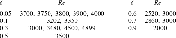
Nonlinear DNS have been performed to confirm the results of the linear stability analysis. The values of
 ${\it\delta}$
and
 $\mathit{Re}$
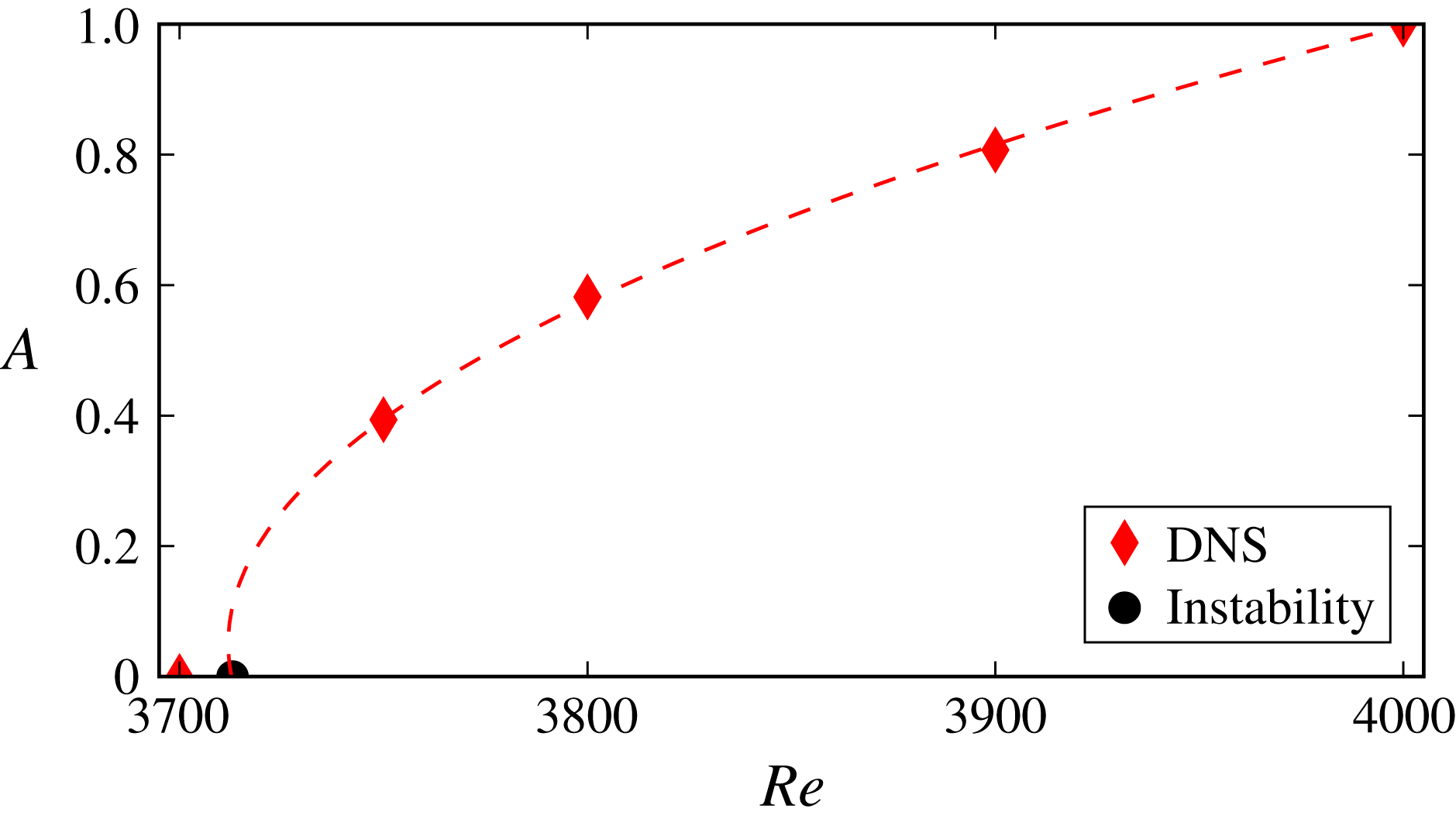
of these simulations are reported in table 1. A randomly perturbed Poiseuille profile was used as the initial condition for all simulations. Each value of curvature investigated has a transition from a steady to a periodic regime, confirming the presence of an Hopf bifurcation. Figure 7 confirms it by depicting the amplitude of saturated flow oscillations as a function of
 $\mathit{Re}$
; the result is
 $A\propto \sqrt{\mathit{Re }-\mathit{ Re }_{c}}$
, characteristic of a Hopf bifurcation (Guckenheimer & Holmes Reference Guckenheimer and Holmes1983). Amongst others, the most relevant quantities used for the comparison are: the critical Reynolds number, the wavenumber of the travelling wave, its symmetry properties, growth rate and temporal frequency. The simulations show excellent agreement with the results of the linear analysis, confirming all properties related to the critical modes. While quantities such as the wavenumber, symmetry, growth rate and temporal frequency could be measured directly, the critical Reynolds number needed to be derived from the other quantities. To do so, the amplitude of the oscillating flow has been measured in simulations across the neutral curve. The envelopes of these oscillations have then been extracted from the time intervals where the signals exhibited exponentially growing, respectively decaying behaviour (depending on
 $\mathit{Re}$
, of course). The time-averaged growth rate and the Reynolds numbers of the two simulations have then been employed in a two-point, linear interpolation to estimate the Reynolds number corresponding to zero growth rate for the nonlinear flow. An example of this procedure is shown in figure 7 for
 ${\it\delta}=0.05$
. For this curvature the interpolation between the DNS for
 $\mathit{Re}=3700$
and
 $3750$
gives
 $\mathit{Re}_{\mathit{c}}\approx 3713.2$
, the linear analysis predicts a critical Reynolds number
 $\mathit{Re}_{\mathit{c}}=3713.36$
. All other quantities compared between nonlinear DNS and the linear analysis are affected by differences of the same order of magnitude.
Saturation amplitude,
 $A$
, measured as a function of Reynolds number for curvature
 ${\it\delta}=0.05$
. The critical Reynolds number is
 $\mathit{Re}_{c}=3713$
. The round (black) marker corresponds to the critical
 $\mathit{Re}$
computed through the linear stability analysis. The dashed line represents a second-order polynomial fit to the DNS data; its intercept with the horizontal axis was computed by linearly interpolating the growth rate, respectively decay, of the oscillations measured in the simulations for
 $\mathit{Re}=3750$
, respectively
 $\mathit{Re}=3700$
.

Values of curvature and Reynolds number at which direct numerical simulations were performed. All DNS were performed in a full, three-dimensional torus.

6 Discussion and conclusions
The present results are compared with the literature in figure 8 (in the range where previous data are available). It can be noted that, in spite of the different methods employed, all previous works indicate subcritical transition for curvatures below 0.02–0.04. This phenomenon was expected since
 ${\it\delta}$
is nearing its lower limit and the effect that the centrifugal force has on the flow becomes less relevant. Moreover, the diameter of the torus is so large in comparison to that of the pipe that the feedback-like mechanism caused by the
 $2{\rm\pi}$
-periodicity in the streamwise direction becomes almost irrelevant to the flow.
Comparison of the neutral curve with experimental and numerical data from the literature. The continuous (black) line represent the envelope of families F4S and F5A (the intersection is at
 ${\it\delta}=0.016$
, where the two dotted lines highlight the continuation of the two families). The data by Cioncolini & Santini (Reference Cioncolini and Santini2006) refers to the first discontinuity in their friction measurements, while the reported data by Sreenivasan & Strykowski (Reference Sreenivasan and Strykowski1983) is the curve they refer to as the ‘conservative lower critical limit’, and that by Noorani & Schlatter (Reference Noorani and Schlatter2015) is for sublaminar friction drag. The interpolants provided by Kühnen et al. (Reference Kühnen, Braunshier, Schwegel, Kuhlmann and Hof2015) are also depicted: with a dashed (blue) line the fit for the supercritical transition and with a dotted (blue) line the fit for subcritical transition. All results agree on subcritical transition for very low curvature, with the data by Kühnen et al. (Reference Kühnen, Braunshier, Schwegel, Kuhlmann and Hof2015) falling on top of that by Sreenivasan & Strykowski (Reference Sreenivasan and Strykowski1983).

Higher curvatures, on the other hand, present a different picture. Both Sreenivasan & Strykowski (Reference Sreenivasan and Strykowski1983) and Kühnen et al. (Reference Kühnen, Braunshier, Schwegel, Kuhlmann and Hof2015) appear to have identified family F4S. The former selected the appearance of the first ‘bursts’ near the outer wall as a definition for the critical Reynolds number. This explains the higher estimate of
 $\mathit{Re}$
where supercritical transition occurs, but also answers their question on the cause behind the non-monotonic behaviour of their data: the switch from subcritical to supercritical transition. Kühnen and coworkers, on the other hand, aware of the supercritical transition identified by Webster & Humphrey (Reference Webster and Humphrey1993), Di Piazza & Ciofalo (Reference Di Piazza and Ciofalo2011), report the Reynolds number corresponding to the onset of the periodic state. These measurements are in fair agreement with F4S. They confirm the relevance of the linear instability and that the first instability is caused by a Hopf bifurcation. The discrepancy in Reynolds number, and the trend of their interpolant may well be due to an optimistic estimate of the accuracy of their measurements, as well as the absence of data at higher curvatures. In fact, the DNS performed at the rightmost point of their dataset,
 ${\it\delta}=0.1,~\mathit{Re}=3202$
, confirms the absence of oscillations.
In conclusion, the toroidal geometry allows the isolation of the effect that
 ${\it\delta}$
has on the first instability. It will now be possible to separate these effects from others when investigating differently curved pipes. Results show that a very little curvature is sufficient to make this flow linearly unstable via a Hopf bifurcation that leads the flow to a periodic regime. The neutral curve associated with this bifurcation has been traced in parameter space exploring, for the first time, the whole range of possible curvatures. The Reynolds number and the wavelength of the critical modes diverge when approaching
 ${\it\delta}=0$
, suggesting a continuous transition to the straight pipe, which has modes with high
 ${\it\lambda}$
, i.e. quasi-streamwise independent, as the least-stable ones.
Acknowledgement
Financial support by the Swedish Research Council (VR) is gratefully acknowledged. Computer time was provided by the Swedish National Infrastructure for Computing (SNIC).