1. Introduction
Liquid jets are widely present in a broad range of natural processes and industrial applications including sea spray, fuel atomisation, controlled drug release, ink-jet printing and flow focusing (Lin Reference Lin2003; Eggers & Villermaux Reference Eggers and Villermaux2008; Ji, Yang & Feng Reference Ji, Yang and Feng2021; Yang et al. Reference Yang, Ji, Ault and Feng2023). The distinct flow regimes, dripping and jetting, determine the operation scenario and significantly influence the performance and efficiency of these processes (Utada et al. Reference Utada, Fernandez-Nieves, Gordillo and Weitz2008). Accordingly, the ability to regulate the flow regimes of a liquid jet and to predict the critical conditions for transition between regimes is of fundamental importance. In recent years, considerable efforts have been devoted to elucidating the physical mechanisms underlying the dripping–jetting transition, with a particular focus on the stability characteristics of the jet flow (Herrada & Montanero Reference Herrada and Montanero2016; Cruz-Mazo et al. Reference Cruz-Mazo, Herrada, Gañán-Calvo and Montanero2017; Ponce-Torres et al. Reference Ponce-Torres, Rebollo-Muñoz, Herrada, Gañán-Calvo and Montanero2018; Montanero & Gañán-Calvo Reference Montanero and Gañán-Calvo2020).
Regarding a capillary-dominated jet, the manifestation of either dripping or jetting regimes is primarily governed by the interplay between inertial and capillary forces (Lin & Lian Reference Lin and Lian1989), quantified by the Weber number, defined as
 ${\textit{We}} = {\rho U^2 R}/{\gamma }$
, where
 $\rho$
denotes the liquid density,
 $U$
is the jet velocity,
 $R$
is the nozzle radius and
 $\gamma$
is the surface tension. In fact, the critical Weber number (
 ${\textit{We}}_c$
) for dripping–jetting transition is always affected by additional factors, one of which is the velocity relaxation of the liquid jet after ejection. At the nozzle exit, the emerging jet often exhibits a non-uniform initial velocity profile (Leib & Goldstein Reference Leib and Goldstein1986b
; Sevilla Reference Sevilla2011; Umemura Reference Umemura2011; Beneitez, Moreno-Boza & Sevilla Reference Beneitez, Moreno-Boza and Sevilla2023), stemming from the no-slip condition imposed at the nozzle wall. As the liquid jet exits into a quiescent gas environment, the shear stress at the jet surface vanishes, and the velocity profile progressively relaxes due to the viscous effect, ultimately approaching a nearly uniform distribution further downstream (Duda & Vrentas Reference Duda and Vrentas1967; Philippe & Dumargue Reference Philippe and Dumargue1991; Oguz Reference Oguz1998; Rohlfs et al. Reference Rohlfs, Ehrenpreis, Haustein and Kneer2014). Meanwhile, this relaxation process is accompanied by a contraction of the jet surface (Gavis & Modan Reference Gavis and Modan1967; Haustein, Harnik & Rohlfs Reference Haustein, Harnik and Rohlfs2017; Beneitez et al. Reference Beneitez, Moreno-Boza and Sevilla2023). Such relaxation-driven flow evolution substantially influences the critical condition for the dripping–jetting transition, which is often responsible for the discrepancies between jets from nozzles of different length/radius ratios (Montessori et al. Reference Montessori, Lauricella, Stolovicki, Weitz and Succi2019).
To quantify the influence of velocity relaxation on the transition between dripping and jetting regimes, basic flow and further stability analyses have been carried out. Leib & Goldstein (Reference Leib and Goldstein1986b
) conducted a local spatio-temporal stability analysis on a liquid jet with velocity relaxation (velocity-relaxation jet) under an inviscid assumption, where the velocity profile is described using a parametric family of functions of
 $(1 - br^2)/(1 - b/2)$
. The parameter
 $b$
was varied from 1 to 0 to represent the progressive relaxation of the velocity profile from an initial parabolic (Poiseuille-like) shape to a uniform distribution, while local stability analyses were performed independently for each velocity profile. Their findings indicate that the transition between regimes is governed by the absolute/convective instability mechanism. It was further shown that most non-uniform velocity profiles act to stabilise the jet by suppressing the disturbance growth rate, ultimately leading to a lower
 ${\textit{We}}_c$
value. However, the employed parametric velocity profiles may fail to faithfully capture the actual velocity distributions observed in practical configurations (Castrejón-Pita et al. Reference Castrejón-Pita, Hoath and Hutchings2012). Sevilla (Reference Sevilla2011) derived a numerical approach to compute the jet basic flow with velocity relaxation, which well captures the inflection point of the velocity profile, a key feature that is absent in the previous parametric representations, under the assumption of high enough Reynolds number (
 ${\textit{Re}} = {\rho U R}/{\mu }\gg 1$
, where
 $\mu$
is the liquid viscosity). On this basis, a local spatio-temporal stability analysis was also performed to determine
 ${\textit{We}}_c$
by identifying the emergence of local absolute instability, and it was reported that the velocity profile has a surprisingly large effect on
 ${\textit{We}}_c$
. Specifically, once
 ${\textit{Re}}$
exceeds about 50,
 ${\textit{We}}_c$
for the jet with an initial Poiseuille profile increases rapidly, eventually surpassing and becoming significantly larger than that for the jet with a uniform velocity profile. This result suggests a qualitative change in the role of viscous relaxation with increasing
 ${\textit{Re}}$
– from suppressing to promoting the growth of disturbances, a conclusion standing in contrast to the qualitative trends reported in other investigations (Leib & Goldstein Reference Leib and Goldstein1986b
; Ibrahim Reference Ibrahim1998; Ibrahim & Marshall Reference Ibrahim and Marshall2000; Söderberg Reference Söderberg2003; Lhuissier, Néel & Limat Reference Lhuissier, Néel and Limat2014). However, there is currently no evidence to support this conclusion, and existing physical models do not identify the factors responsible for the reversal of the velocity relaxation effect. Therefore, previous theoretical models need to be validated by comparative experiments under conditions with and without velocity relaxation, and the role of velocity relaxation in the dripping–jetting transition remains to be clarified further.
To this end, we experimentally measured the critical Weber number,
 ${\textit{We}}_c$
, of capillary jets with initial Poiseuille and uniform velocity profiles, i.e. capillary jets with and without velocity relaxation, respectively. Our results show the velocity relaxation consistently lowers
 ${\textit{We}}_c$
, which contrasts with the predictions of the classic local spatio-temporal stability analysis. To elucidate the underlying physics of this phenomenon, we revisit the velocity-relaxation jet using a global stability framework, and explore the global dynamics of the jet instability during the dripping–jetting transition. The subsequent sections are organised as follows. Section 2 presents the experimental methodology and measurements of
 ${\textit{We}}_c$
. In § 3, a global stability model for the velocity-relaxation jet is developed. Section 4 discusses the theoretical predictions of
 ${\textit{We}}_c$
and compares them with experimental results. Finally, the main conclusions are summarised in § 5.
2. Experimental details
The experimental set-up is illustrated in figure 1(a). The working fluid was deionised water, with a density of
 $\rho = 997$
kg m
 $^{-3}$
, dynamic viscosity
 $\mu = 0.89$
mPa s and surface tension
 $\gamma = 71.6 \pm 1.0$
mN m
 $^{-1}$
. The jet was driven by a syringe pump (Pump 33 DDS, Harvard Apparatus), which provided precise control over the volumetric flow rate
 $Q$
as well as the flux-averaged velocity
 $U = Q/(\pi R^2)$
. Instead of continuously varying the flow rate, a series of discrete, steady-state flow conditions were imposed, allowing sufficient time for the flow to settle and avoiding the transient effects associated with regime transition. The nozzles were kept dry before injection to prevent exit wetting and maintain a pinned contact line at the outlet inner edge. The final flow state of the jet under each flow rate was recorded after a prolonged period (at least 5 s) of constant flow. The jet behaviour was visualised using a high-speed camera (FASTCAM Mini AX200, Photron) equipped with a 100 mm f/2.8 macro lens (Tokina), operating at 5000 frames per second with an exposure time of 10
 $\unicode {x03BC}$
s and a spatial resolution of 28
 $\unicode {x03BC}$
m per pixel, under the illumination of an LED panel background light source. The experiments were conducted at 25
 $^{\circ }$
C and 1 atm.
To eliminate uncertainties associated with varying degrees of velocity profile development, the nozzles were selected to be sufficiently long to ensure that the internal flow had fully developed into a Poiseuille flow, and the corresponding jet is referred to as the Poiseuille-velocity jet. Accordingly, the minimum nozzle length was constrained to exceed the development length of the inner flow, calculated as
 $l_{{min}} = 0.16ReR$
(Lew & Fung Reference Lew and Fung1970). Additionally, according to the definitions of the dimensionless numbers
 ${\textit{We}}$
and
 ${\textit{Re}}$
, once the working fluid is fixed, a nozzle with a given radius corresponds to only one (
 ${\textit{Re}}$
,
 ${\textit{We}}_c$
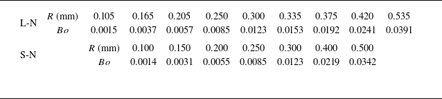
) pair. Therefore, a set of long nozzles (L-N) with various radii, as presented in table 1, were employed to adjust
 ${\textit{Re}}$
. Notably, to minimise the gravitational effect, the Bond number (
 $Bo = {\rho g R^2}/{\gamma }$
, where
 $g = 9.81$
m s
 $^{-2}$
) was maintained below 0.04 in all cases. Finally, to isolate the impact of velocity relaxation, a set of short nozzles (S-N) with similar radii were used as a control group (table 1), where the nozzle exit length
 $l$
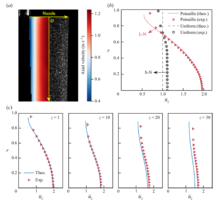
is only 0.5 mm thus approximating the jet with a uniform velocity distribution, which is referred to as the uniform-velocity jet. The initial velocity profiles generated by L-N and S-N were measured via particle image velocimetry (PIV), detailed in Appendix A.
Inner radius of long (L-N) and short (S-N) nozzles and the corresponding values of
 $Bo$
.

Experimental investigation of the dripping–jetting transition of velocity-relaxation jets. (a) Schematic of the experimental apparatus. The nozzle has an inner radius of
 $R$
and an exit length of
 $l$
. (b) Representative image sequences showing the variation of jet breakup length
 $L_b$
with increasing
 ${\textit{We}}$
. The red dashed line outlines the general trend of the breakup length variation. (c) Mean breakup length as a function of
 ${\textit{We}}$
. The red symbols and blue shading highlight the stage of rapid variation in the breakup length, defined as the transition interval between the dripping and jetting regimes. Here,
 ${\textit{We}}_1$
and
 ${\textit{We}}_2$
denote the upper and lower thresholds of this interval, corresponding to the onset of the sudden decrease and sudden increase in
 $L_b$
, respectively. Typical videos of the jet flow in dripping and jetting regimes are provided in supplementary movies 1 and 2, available at https://doi.org/10.1017/jfm.2025.11045.

Figure 1(b) illustrates the typical features of the instability and breakup of a Poiseuille-velocity jet from a nozzle of
 $R = 0.250$
mm at different
 ${\textit{We}}$
. When
 ${\textit{We}}$
is small (1.838–2.046), the detachment location of the jet is close to the nozzle exit, and the breakup length
 $L_b$
increases slowly with
 ${\textit{We}}$
, a trend also apparent in figure 1(c). At this regime, the jet exhibits pronounced self-excited oscillations (Umemura & Osaka Reference Umemura and Osaka2014; Umemura Reference Umemura2016). Tip contraction upon each breakup event generates reverse-propagating capillary waves travelling upstream towards the nozzle, as captured in figure 2. These disturbances subsequently evolve into secondary wave packets, giving rise to multiple breakup events downstream (see supplementary movie 1 available at https://doi.org/10.1017/jfm.2025.11045). Such behaviour is indicative of a quasi-periodic or chaotic regime, consistent with the so-called ‘dripping faucet’ mode described by Clanet & Lasheras (Reference Clanet and Lasheras1999). Although distinct from the classic ‘periodic dripping’, this state is still classified within the dripping regime. As
 ${\textit{We}}$
increases beyond the lower threshold
 ${\textit{We}}_2 = 2.046$
, the breakup length
 $L_b$
rises sharply until the upper threshold
 ${\textit{We}}_1 = 2.220$
is reached (figure 1
c). Thereafter,
 $L_b$
stabilises and returns to a trend of slow growth with
 ${\textit{We}}$
(Zhang et al. Reference Zhang, Shi, Sun, Liu, Li, Yang, Fu and Ji2025), indicating a complete transition into the jetting regime (see supplementary movie 2). Following the classic criterion (Clanet & Lasheras Reference Clanet and Lasheras1999; Ambravaneswaran et al. Reference Ambravaneswaran, Subramani, Phillips and Basaran2004), we similarly identify the sudden variation in
 $L_b$
as the onset of regime transition. To avoid confusion between dripping-to-jetting and jetting-to-dripping processes, we define the critical Weber number as the mean of the transition interval, i.e.
 ${\textit{We}}_c = ({\textit{We}}_1 + {\textit{We}}_2)/2$
, and denote
 $[{\textit{We}}_2, {\textit{We}}_1]$
as the confidence interval.
Time sequences showing the instability and breakup process of a capillary jet in the dripping faucet regime, from a long nozzle with an inner radius of
 $R=0.250$
mm at
 ${\textit{We}} = 1.879$
. The time interval between consecutive frames is 0.4 ms. The red arrow indicates the upward propagation of the reverse waves initiated from the tip contraction upon breakup. These disturbances subsequently evolve and trigger a sequence of four breakup events, marked by the blue arrows and accompanying annotations (also see supplementary movie 1).

Based on this transition criterion,
 ${\textit{We}}_c$
for both Poiseuille- and uniform-velocity jets were measured, as presented in figure 3. For comparison, theoretical predictions for both jets based on local spatio-temporal stability analysis are included (Sevilla Reference Sevilla2011; Leib & Goldstein Reference Leib and Goldstein1986a
). First, it shows that the experimentally measured
 ${\textit{We}}_c$
for the uniform-velocity jet exhibits excellent agreement with the theoretical results of the local model. This not only validates the experimental methodology and transition criterion adopted, but also confirms that, in the range of
 $R \leqslant 0.5$
mm, the gravitational stretching effect of the deionised water jet can be safely ignored. Second, the measured
 ${\textit{We}}_c$
of the Poiseuille-velocity jet remains consistently lower than that of counterparts with uniform-velocity profiles, indicating that velocity relaxation persistently suppresses the jet instability within the parameter range of this study. In stark contrast to the predictions of local stability theory, the experimental
 ${\textit{We}}_c$
for Poiseuille-velocity jets is significantly lower and shows increasing deviation from the local model with rising
 ${\textit{Re}}$
. Notably, under high Reynolds numbers (
 ${\textit{Re}} \geqslant 143$
), the local theory not only overestimates the values of
 ${\textit{We}}_c$
, but also incorrectly predicts an enhancing effect of velocity relaxation on the jet instability. These substantial discrepancies indicate that the classic local stability analysis is inadequate for predicting the regime transition conditions of velocity-relaxation jets, particularly under high-
 ${\textit{Re}}$
conditions.
As postulated by Huerre & Monkewitz (Reference Huerre and Monkewitz1990), global stability may play a central role in governing the transition between dripping and jetting regimes. For jets with an initial non-uniform velocity distribution, the ejection process leads to velocity relaxation and radial contraction, resulting in a strongly non-parallel and non-uniform basic flow, whose spatial scale may be comparable to that of the disturbance. Under such conditions, the fundamental parallel-flow assumption of local stability theory is likely violated (Montanero & Gañán-Calvo Reference Montanero and Gañán-Calvo2020). In contrast, global stability analysis can offer a more comprehensive framework to capture the pronounced non-parallelism of both the basic flow and the evolving disturbances (Gordillo, Sevilla & Campo-Cortés Reference Gordillo, Sevilla and Campo-Cortés2014; Herrada & Montanero Reference Herrada and Montanero2016). Indeed, global analysis has demonstrated marked advantages in predicting flow behaviour in various non-parallel flows, such as jets subjected to electric fields (Ponce-Torres et al. Reference Ponce-Torres, Rebollo-Muñoz, Herrada, Gañán-Calvo and Montanero2018; Liu et al. Reference Liu, Ji, Zou, Zhang, Sun, Fu and Yang2025) or gravitational stretching (Sauter & Buggisch Reference Sauter and Buggisch2005; Rubio-Rubio, Sevilla & Gordillo Reference Rubio-Rubio, Sevilla and Gordillo2013; Shukla & Gallaire Reference Shukla and Gallaire2020; Sun et al. Reference Sun, Liu, Zhang, Ji, Yang and Fu2024b ), as well as in flow-focusing systems (Gordillo et al. Reference Gordillo, Pérez-Saborid and Gañán-Calvo2001, Reference Gordillo, Sevilla and Campo-Cortés2014; Gañán-Calvo Reference Gañán-Calvo2008; Tammisola, Lundell & Söderberg Reference Tammisola, Lundell and Söderberg2012; Cruz-Mazo et al. Reference Cruz-Mazo, Herrada, Gañán-Calvo and Montanero2017; Schmidt et al. Reference Schmidt, Tammisola, Lesshafft and Oberleithner2021). These precedents suggest that the discrepancy observed between the experiments and theoretical predictions in figure 3 likely stems from the inherent limitations of local stability analysis. Therefore, adopting a global perspective is essential for accurately characterising the dynamics of velocity-relaxation jets.
Comparison between experimental measurements and theoretical
 ${\textit{We}}_c$
through local stability analysis. The black solid and purple dashed lines denote the theoretical predictions for a Poiseuille-velocity jet by Sevilla (Reference Sevilla2011) and a uniform-velocity jet by Leib & Goldstein (Reference Leib and Goldstein1986a
), respectively. The
 ${\textit{Re}}$
values increase monotonically with the nozzle radii in table 1. The error bars represent the confidence intervals
 $[{\textit{We}}_2, {\textit{We}}_1]$
, where both the upper and lower thresholds are taken as the means of three repeated experiments.

3. Global stability analysis
A mathematical model, illustrated in figure 4, is formulated with the origin of the cylindrical coordinate system located at the centre of the nozzle exit. We consider an axisymmetric liquid jet with an initial velocity profile at the nozzle exit following the classic Poiseuille form,
 $\bar {u}_z( z=0,r ) =2U( 1-{{r^2}/{R^2}} )$
, where
 $\bar {u}_z$
denotes the steady axial component of the velocity field
 $\boldsymbol{u}=[ u_z( z,r,t ) ,0,u_r( z,r,t ) ] ^{\mathrm{T}}$
. To account for the contraction of the jet surface induced by velocity relaxation, the local jet radius is modelled as a function of both axial position and time, i.e.
 $h( z,t )$
. Due to the low
 ${\textit{We}}$
in our experiments and the small density and viscosity ratios of gas to liquid, aerodynamic shear effects from the quiescent ambient gas are neglected (Ibrahim & Marshall Reference Ibrahim and Marshall2000), and only the intrinsic hydrodynamic relaxation of the jet is considered. Gravitational acceleration is also omitted due to its negligible influence at small enough
 $Bo$
. The physical variables in this system, such as velocity, length, time and pressure
 $p$
, are rendered dimensionless using the characteristic scales
 $U$
,
 $R$
,
 ${R}/{U}$
and
 $\rho U^2$
, respectively.
Sketch of a velocity-relaxation jet.

The jet with velocity relaxation is modelled as the superposition of a steady basic flow and a small-amplitude linear disturbance. The disturbance is treated as a two-dimensional global mode, with the entire jet system oscillating harmonically at a common complex frequency
 $\omega$
, independent of disturbance components and spatial positions (Chomaz Reference Chomaz2005; Theofilis Reference Theofilis2011; Montanero & Gañán-Calvo Reference Montanero and Gañán-Calvo2020). The global flow field is thus represented in the form of
 \begin{equation} \boldsymbol{\phi }( z,r,t ) =\bar {\boldsymbol{\phi }}( z,r ) +\varepsilon \hat {\boldsymbol{\phi }}( z,r ) \exp ( \omega t ) , \end{equation}
where
 $\boldsymbol{\phi }=[ u_z, u_r, p, h ] ^{\mathrm{T}}$
denotes a vector consisting of different scalar flow variables and
 $\bar {\boldsymbol{\phi }}$
and
 $\hat {\boldsymbol{\phi }}$
represent the components corresponding to the steady basic flow and the linear disturbance, respectively. The parameter
 $\varepsilon$
is assumed to be a small quantity (
 $\varepsilon \ll 1$
). The complex frequency
 $\omega$
characterises the global mode, where its real part
 $\mathcal{R}(\omega )$
corresponds to the temporal growth rate of the disturbance and its imaginary part
 $\mathcal{I}(\omega )$
represents the oscillation frequency. When
 $\mathcal{R}(\omega ) \lt 0$
, the disturbance
 $\hat {\boldsymbol{\phi }}$
decays exponentially over time, indicating that the basic flow
 $\bar {\boldsymbol{\phi }}$
is linearly asymptotically stable. Conversely, if
 $\mathcal{R}(\omega ) \gt 0$
, the disturbance grows exponentially and eventually leads to jet breakup, indicating that the basic flow is linearly unstable.
Notably, both local and global stability models can account for the non-uniform basic flow
 $\bar {\boldsymbol{\phi }}$
resulting from velocity relaxation, but the global framework has the further advantage of capturing the non-uniform and non-parallel effects of the disturbance
 $\hat {\boldsymbol{\phi }}$
(Juniper, Hanifi & Theofilis Reference Juniper, Hanifi and Theofilis2014; Montanero & Gañán-Calvo Reference Montanero and Gañán-Calvo2020). In local theory, the disturbance is assumed to take a normal-mode form (Sun et al. Reference Sun, Cui, Zhang, Liu, Yang, Ji and Fu2024a
), i.e.
 $\hat {\boldsymbol{\phi }}(z,r) = \hat {\boldsymbol{\phi }}_1(r) \exp (kz)$
, where the real and imaginary parts of the complex wavenumber
 $k$
,
 $\mathcal{R}(k)$
and
 $\mathcal{I}(k)$
, represent the spatial growth rate and axial wavenumber, respectively. Under this assumption, the disturbances at different
 $r$
locations of the same
 $z$
location are forced to follow the same exponential growth law
 $\exp (kz)$
(Leib & Goldstein Reference Leib and Goldstein1986b
; Sevilla Reference Sevilla2011), regardless the uniformity of the initial velocity distribution and the extent of velocity relaxation. In contrast, in the global model (3.1), the disturbance
 $\hat {\boldsymbol{\phi }}$
is treated as a two-dimensional field, which can vary along both
 $r$
and
 $z$
directions. The two-dimensional variable
 $\hat {\boldsymbol{\phi }}(z,r)$
can therefore capture the full spatial development of the disturbance, including coupling between axial and radial components and non-exponential spatial growth, which may better represent the actual flow, especially for a jet with non-uniform velocity profiles. This means that the global stability analysis can provide more accurate theoretical predictions for the non-uniform flows of velocity-relaxation jets as we show below.
Substituting (3.1) into the two-dimensional continuity and Navier–Stokes equations and neglecting the high-order terms regarding
 $\varepsilon \ll 1$
, we can obtain the linearised governing equations enabling us to incorporate the effects of velocity relaxation, i.e.
 \begin{align} \hat {u}_{z,z} +\hat {u}_{r,r}+{{\hat {u}_r}/{r}}=0 , \\[-8pt] \nonumber \end{align}
 \begin{align} -\bar {u}_z\hat {u}_{z,z}-\bar {u}_{z,r}\hat {u}_r-\bar {u}_{z,z}\hat {u}_z-\bar {u}_r\hat {u}_{z,r}-\hat {p}_{,z}+Re^{-1} ( \hat {u}_{z,zz}+\hat {u}_{z,rr}+{{\hat {u}_{z,r}}/{r}} ) &=\omega \hat {u}_z , \end{align}
 \begin{align} -\bar {u}_z\hat {u}_{r,z}-\bar {u}_{r,r}\hat {u}_r-\bar {u}_r\hat {u}_{r,r}-\hat {p}_{,r}+Re^{-1} ( \hat {u}_{r,zz} + \hat {u}_{r,rr} + {{\hat {u}_{r,r}}/{r}} - {{\hat {u}_r}/{r^2}} ) &=\omega \hat {u}_r , \end{align}
where commas in the subscripts denote partial derivatives with respect to the corresponding spatial coordinates. For instance,
 $\hat {u}_{z,z}$
represents the derivative of the axial velocity disturbance
 $\hat {u}_z$
with respect to
 $z$
. The steady velocity components,
 $\bar {u}_z$
and
 $\bar {u}_r$
, are obtained numerically following the basic flow model of Sevilla (Reference Sevilla2011), under the assumption of
 ${\textit{Re}} \gg 1$
. The theoretical results of the basic flow were verified by our PIV experiments, as detailed in Appendix A. Note that for low-
 ${\textit{Re}}$
conditions (
 ${\textit{Re}} \sim O(1)$
), the error of this simplified basic flow may increase, in which case a more complete steady model, such as the JAM framework developed by Herrada & Montanero (Reference Herrada and Montanero2016), may serve as an appropriate alternative.
At the jet surface
 $r=h( z,t )$
, the following two dynamic boundary conditions should be satisfied: (i) the tangential stress vanishes due to the neglected shear effect from the ambient gas; (ii) the normal stress difference should be in balance to the surface tension. These conditions yield
 \begin{align} \hat {u}_{z,r}+\hat {u}_{r,z}+\bar {u}_{z,rr}\hat {h}+2\bar {h}_{,z}( \hat {u}_{r,r}-\hat {u}_{z,z} ) +2( \bar {u}_{r,r}-\bar {u}_{z,z} ) \hat {h}_{,z}=0 \quad \mbox{at} \quad r &= \bar {h} (z) , \end{align}
 \begin{align} \hat {p}-2\hat {u}_{r,r} + We^{-1} ( \bar {h}^{-2}\hat {h} + \bar {h}^{-1} \bar {h}_{,z}\hat {h}_{,z} + \hat {h}_{,zz} ) =0 \quad \mbox{at} \quad r = \bar {h} (z) . \end{align}
Additionally, the kinematic boundary condition should ensure the relationship between the jet surface and velocity, yielding
 \begin{equation} -\bar {u}_z\hat {h}_{,z}-\bar {h}_{,z}\hat {u}_z+\bar {u}_{r,r}\hat {h}+\hat {u}_r =\omega \hat {h} \quad \mbox{at} \quad {r = \bar {h} (z)} . \end{equation}
To ensure the closure of the differential system described by (3.2)–(3.7), additional boundary conditions should be imposed. At the jet axis (
 $r=0$
), the axisymmetric condition requires
 $\hat {u}_r=\hat {u}_{z,r}=\hat {p}_{,r}=0$
. At the nozzle exit (
 $z=0$
), zero initial disturbance is imposed such that
 $\hat {u}_z=\hat {u}_r= \hat {p}=\hat {h}=0$
. At the downstream cutoff boundary (
 $z=L_z$
), soft outflow conditions (Montanero & Gañán-Calvo Reference Montanero and Gañán-Calvo2020) are applied such that
 $\hat {u}_{z,z} =\hat {u}_{r,z} =\hat {h}_{,z}=0$
, which has been proven not to affect the accuracy of the results as long as the axial computational domain
 $L_z$
is sufficiently large (Rubio-Rubio et al. Reference Rubio-Rubio, Sevilla and Gordillo2013; Shukla & Gallaire Reference Shukla and Gallaire2020), as detailed in Appendix B.
To numerically solve this global stability problem, a generalised eigenvalue approach,
 $ \boldsymbol{A} \hat {\boldsymbol{\phi }} = \omega \boldsymbol{B} \hat {\boldsymbol{\phi }}$
, is employed to compute the eigenvalue
 $\omega$
and its corresponding eigenvector
 $\hat {\boldsymbol{\phi }}$
, where the coefficient matrices
 $\boldsymbol{A}$
and
 $\boldsymbol{B}$
are determined by the governing equations (3.2)–(3.4) and boundary conditions (3.5)–(3.7). The two-dimensional disturbance is discretised using the Chebyshev collocation method in the radial direction and the finite-difference method in the axial direction. The discrete values of all disturbance variables are assembled into a single-column vector, resulting in an eigenvector
 $\hat {\boldsymbol{\phi }}$
of size
 $( 3N_r+1 ) N_z\times 1$
, where
 $N_r$
and
 $N_z$
denote the number of collocation points in the radial and axial directions, respectively. A corresponding two-dimensional differentiation matrix is constructed to perform the spatial derivative operations. Due to the jet surface contraction during the velocity relaxation process, the radial computational domain,
 $[ 0,\bar {h} ]$
, gradually shrinks along the axial direction. To account for this, a coordinate transformation
 $r(z)={{( 1-\xi ) \bar {h}( z )}/{2}}$
is introduced to map the collocation points
 $\xi \in [-1,1]$
onto the physically varying radial domain.
Once the basic flow field of the velocity-relaxation jet is substituted into the generalised eigenvalue problem as a precondition, the complete set of eigenvalues
 $\omega$
and corresponding eigenvectors
 $\hat {\boldsymbol{\phi }}$
for the discretised system can be obtained using standard MATLAB routines. Typically, the eigenvalue with the largest temporal growth rate is regarded as the leading global mode. Nevertheless, in some cases, many spurious eigenvalues may possess growth rates larger than that of the physical leading mode. Thus, to ensure the correct identification of the leading eigenvalue and to filter out spurious solutions, convergence tests should be carried out by varying the numerical parameters
 $N_z$
,
 $N_r$
and
 $L_z$
(see Appendix B), which is a common strategy in selecting the true leading mode of global instability (Shukla & Gallaire Reference Shukla and Gallaire2020).
4. Results and discussion
4.1. Flow evolution and distribution
Figure 5(a) presents the velocity profiles of the basic flow at different axial positions
 $z$
. Since the radial velocity
 $\bar {u}_r$
is
 $O(Re^{-1})$
, much smaller than the axial velocity
 $\bar {u}_z \sim O(1)$
(Sevilla Reference Sevilla2011), only the relaxation of
 $\bar {u}_z$
is shown here. Correspondingly, the relative difference between the maximum and minimum axial velocities at each cross-section,
 $\Delta \bar {u}_z(z)$
, is given by figure 5(b). It shows that the jet’s velocity relaxation process depends solely on the ratio of the axial coordinate
 $z$
to the Reynolds number
 ${\textit{Re}}$
for a given
 ${\textit{We}}$
, under the assumption of
 ${\textit{Re}}\gg 1$
. This indicates that the dimensionless relaxation length of the velocity profile remains of
 $O(Re)$
(Sevilla Reference Sevilla2011; Castrejón-Pita et al. Reference Castrejón-Pita, Hoath and Hutchings2012; Rohlfs et al. Reference Rohlfs, Ehrenpreis, Haustein and Kneer2014). As
 ${\textit{Re}}$
increases, the relaxation length becomes longer, leading to stronger non-parallel and non-uniform effects in the jet flow field.
Numerical results of the basic flow and global stability analysis for (a–e) Poiseuille- and (f) uniform-velocity jets. (a) Axial velocity profiles at different axial locations. The corresponding axial locations (i–v) are marked in (b). (b) Relative difference between the maximum and the minimum axial velocity in each cross-section, defined as
 $\Delta \bar {u}_z(z) = 1 - \bar {u}_z(z,r=\bar {h}) / \bar {u}_z(z,r=0)$
. (c) Eigenvalue spectrum of the global stability analysis. The two leading eigenvalues enclosed by circles are complex conjugates. In (a–c),
 ${\textit{We}}=1.00$
and
 ${\textit{Re}}=50$
. (d–f) Spatial distribution of the real part of the axial velocity disturbance,
 $\mathcal{R} ( \hat {u}_z )$
, corresponding to the leading mode at
 ${\textit{We}}=1.00$
, with
 ${\textit{Re}}=50$
(d) and 1000 (e,f). The blue dashed and solid lines trace
 $\mathcal{R} ( \hat {u}_z )$
along the jet axis
 $r=0$
and surface
 $r=\bar {h}$
, respectively. The black dot-dash lines denote the surface of the basic flow,
 $\bar {h}( z )$
.

On this basis, the eigenvalue spectrum of the global disturbance can be obtained, as shown in figure 5(c) for a Poiseuille-velocity jet with
 ${\textit{We}}=1.00$
and
 ${\textit{Re}}=50$
. The sign of the temporal growth rate
 $\mathcal{R}(\omega )$
is then used to determine the stability of the basic flow. Further, the spatial distribution of the leading disturbance can be obtained from its corresponding eigenvector. As an example, the real part of the axial velocity disturbance,
 $\mathcal{R} ( \hat {u}_z )$
, at various spatial locations
 $( z,r )$
is illustrated by the contour plots in figures 5(d) and 5(e), with
 ${\textit{Re}}=50$
and 1000, respectively. Specifically, when
 ${\textit{Re}}$
is small (
 ${\textit{Re}}=50$
), the disturbance
 $\mathcal{R} ( \hat {u}_z )$
of the Poiseuille-velocity jet exhibits an approximately uniform distribution along the radial direction, as shown by the coloured strips nearly parallel to each other in figure 5(d). This indicates that the development of the disturbance along the axial direction is almost independent of the radial position, suggesting a near-parallel flow. The overlap of the curves of
 $\mathcal{R} ( \hat {u} )$
at
 $r=0$
and
 $r=\bar {h}$
is further evidence of this. In this case, the axial and radial components of the disturbance can be considered separable, i.e.
 $\hat {\phi } ( z,r ) \approx \hat {\phi }_1( r ) \hat {\phi }_2( z )$
. Assuming the axial evolution of the disturbance as a normal mode, i.e.
 $\hat {\phi }_2(z) = \exp ( kz )$
, the global stability analysis degenerates to the local stability theory. Therefore, under low-
 ${\textit{Re}}$
conditions, the global and local models of the Poiseuille-velocity jet can be considered approximately equivalent.
As
 ${\textit{Re}}$
increases, the strongly non-parallel nature of the basic flow causes the spatial distribution of disturbance to become more inhomogeneous, thereby inducing coupling between the axial and radial components of the disturbance function
 $\boldsymbol{\hat {\phi }}(z,r)$
. As shown in figure 5(e) with
 ${\textit{Re}}=1000$
, the strips in the contour plot become distorted and are accompanied by a change in the colour shade. This means that the axial evolution of the disturbance at different radial positions exhibits variations in phase, wavelength, amplitude and spatial growth rate, as indicated by the discrepancy of
 $\mathcal{R} ( \hat {u} )$
at
 $r=0$
and
 $r=\bar {h}$
. For instance, the crests and troughs of the disturbance waveforms display spatial hysteresis nearer the jet surface. In addition, both the amplitude and spatial growth rate of the disturbance tend to increase with
 $r$
, indicating that fluctuations near the jet surface are stronger than those along the axis. In short, the disturbance wave
 $\boldsymbol{\hat {\phi }}(z,r)$
varies with the radial position
 $r$
, suggesting a non-parallel flow. In contrast, at high
 ${\textit{Re}}$
, the absence of velocity relaxation in the uniform-velocity jet causes the two-dimensional global disturbance to revert to a parallel state, as shown in figure 5(f). Thus, beyond the basic flow itself, the non-parallel nature of the disturbance in Poiseuille-velocity jets is a critical feature distinguishing them from uniform-velocity jets, particularly at high
 ${\textit{Re}}$
. However, as noted in § 3, such non-parallel disturbance cannot be properly captured within a local stability framework. This limitation constitutes a key distinction between the global and local models and causes the local model’s failure to accurately predict the stability behaviour of Poiseuille-velocity jets as we discuss below.
4.2. Leading growth rate and critical Weber number
Figure 6 illustrates the variation of the temporal growth rate of the leading mode,
 $\mathcal{R}(\omega )$
, as a function of the dimensionless parameters
 ${\textit{We}}$
and
 ${\textit{Re}}$
. It is evident that
 $\mathcal{R}(\omega )$
decreases with increasing
 ${\textit{We}}$
or decreasing
 ${\textit{Re}}$
, indicating that surface tension exerts a stabilising effect on the jet, while liquid viscosity acts to dampen the growth of disturbances. Furthermore, a comparison between jets with different initial velocity profiles reveals that velocity relaxation suppresses the disturbance growth, thereby enhancing overall jet stability. This stabilising effect of velocity relaxation remains qualitatively consistent across the full range of
 ${\textit{We}}$
and
 ${\textit{Re}}$
explored in this study, aligning with the experimental observations reported in § 2. Notably, the influence of velocity relaxation becomes more pronounced at higher
 ${\textit{We}}$
and lower
 ${\textit{Re}}$
, suggesting that jets with lower surface tension and higher viscosity are more sensitive to variations in the velocity profile.
Temporal growth rate of the leading mode
 $\mathcal{R}(\omega )$
as a function of (a)
 ${\textit{We}}$
at
 ${\textit{Re}} = 100$
and (b)
 ${\textit{Re}}$
at
 ${\textit{We}} = 2.00$
for both Poiseuille- and uniform-velocity jets. The red markers indicate the critical points at which the temporal growth rate crosses zero, with the corresponding
 ${\textit{We}}$
defined as
 ${\textit{We}}_c$
. The purple and orange shaded regions represent the unstable (
 $\mathcal{R}(\omega )\gt 0$
) and stable (
 $\mathcal{R}(\omega )\lt 0$
) regimes, respectively.

To predict the critical Weber number (
 ${\textit{We}}_c$
) for the dripping–jetting transition using the global stability model, a connection must be established between the theoretical stability state and the experimentally observed flow regimes. As defined in (3.1), when the jet is in a linearly stable state (
 $\mathcal{R}(\omega ) \lt 0$
), all perturbations to the basic flow decay exponentially over time. Although actual capillary jets almost always eventually break up into droplets due to convective instability, in this study we imposed a cutoff boundary (
 $z = L_z$
) to restrict the computational domain to the relatively smooth upstream region. This theoretical treatment constructs a finite stable jet, which is a common approach in linear global stability analysis (Rubio-Rubio et al. Reference Rubio-Rubio, Sevilla and Gordillo2013; Gordillo et al. Reference Gordillo, Sevilla and Campo-Cortés2014; Montanero & Gañán-Calvo Reference Montanero and Gañán-Calvo2020; Shukla & Gallaire Reference Shukla and Gallaire2020; Sun et al. Reference Sun, Liu, Zhang, Ji, Yang and Fu2024b
). Thus, the globally stable state in our theoretical model corresponds to the jetting regime. Conversely, if any global mode becomes unstable (
 $\mathcal{R}(\omega ) \gt 0$
), the disturbances, which may originate from flow pulsations, nozzle exit excitations, oscillations due to downstream breakup and so on (Umemura & Osaka Reference Umemura and Osaka2014; Umemura Reference Umemura2016), can amplify and drive the system into a self-excited oscillatory state, ultimately transitioning into the dripping regime (Montanero & Gañán-Calvo Reference Montanero and Gañán-Calvo2020). In other words, dripping is the natural outcome of a globally unstable flow. Accordingly, for a given
 ${\textit{Re}}$
,
 ${\textit{We}}_c$
is defined as the value of
 ${\textit{We}}$
at which
 $\mathcal{R}(\omega ) = 0$
, delineating the boundary between dripping and jetting regimes predicted by global stability analysis (Le Dizès Reference Le Dizès1997; Rubio-Rubio et al. Reference Rubio-Rubio, Sevilla and Gordillo2013; Martínez-Calvo et al. Reference Martínez-Calvo, Rubio-Rubio and Sevilla2018).
Comparison of the critical Weber number (
 ${\textit{We}}_c$
) for dripping–jetting transition predicted by the global stability model with (a) the prediction of local theoretical model and (b) the experimental measurements. The black dot-dash and the red solid lines denote
 ${\textit{We}}_c$
of the Poiseuille-velocity jet predicted by Sevilla (Reference Sevilla2011) based on local spatio-temporal stability analysis and by our global stability model, respectively. The purple dashed and the green solid lines represent
 ${\textit{We}}_c$
of the uniform-velocity jet predicted by the local stability model by Leib & Goldstein (Reference Leib and Goldstein1986a
) and by our global stability model, respectively. Weak (WVR) and strong velocity-relaxation (SVR) regions are divided by
 ${\textit{Re}} = 43$
. The light red and green long-dashed lines in (b) are the fitted models (4.1) and (4.2), respectively.

4.3. Dripping–jetting transition considering velocity relaxation
Figure 7(a) presents the predicted
 ${\textit{We}}_c$
at various
 ${\textit{Re}}$
for both uniform- and Poiseuille-velocity jets calculated by different stability models. Applying our global stability analysis of the capillary jet with an initial uniform velocity profile, we obtain results showing good agreement with the prediction of local spatio-temporal stability analysis by Leib & Goldstein (Reference Leib and Goldstein1986a
), as well as the experimental results with short nozzles (figure 7
b). As shown in figure 5(f), once the basic flow field is uniform, the global disturbance should be able to degenerate into the normal mode in the local theory, indicating the equivalence of the two models. This degradation operation can partially validate the theoretical framework and numerical methods for the global stability analysis proposed in § 3.
In contrast, for a Poiseuille-velocity jet, a notable discrepancy arises between the predictions of the global stability analysis and those of the local model (Sevilla Reference Sevilla2011), and this discrepancy grows with increasing
 ${\textit{Re}}$
. Moreover, the effect of velocity relaxation on jet instability differs qualitatively between the two models. While the local model predicts
 ${\textit{We}}_c$
for Poiseuille-velocity jets that first falls below and then exceeds that of the uniform-velocity jet with increasing
 ${\textit{Re}}$
, the global stability model consistently yields a lower
 ${\textit{We}}_c$
for the Poiseuille-velocity jet. Figure 7(b) shows that the relative deviation between our theoretical predictions and the experiments remains below 10 % over a wide range of
 ${\textit{Re}}$
, which is considerably smaller than that obtained with the local model. This demonstrates that our global stability model provides more accurate predictions of
 ${\textit{We}}_c$
for the Poiseuille-velocity jet than the local stability model.
At a high
 ${\textit{Re}}$
, the jet flow with velocity relaxation features pronounced non-parallel and non-uniform characteristics, especially for the jet disturbance, as illustrated in figure 5(e). Physically, the non-parallel and non-uniform velocity disturbances inevitably cause velocity differences across
 $r$
, inducing stronger interlayer drag and viscous dissipation, thereby suppressing the disturbance growth. In the energy budget of jet disturbances, viscous shear invariably extracts energy from the perturbation field, diminishing the disturbance kinetic energy. As this energy determines the growth rate, non-parallel global disturbances ultimately suppress disturbance amplification and stabilise the entire jet system. This means that the velocity relaxation consistently reduces
 ${\textit{We}}_c$
of the liquid jet and further illustrates the physical irrationality of the local stability results. Thus, to precisely predict the critical Weber number for liquid jets with velocity relaxation, the disturbance must be treated as a globally evolving, two-dimensional structure rather than as a collection of locally evolving, one-dimensional modes.
As
 ${\textit{Re}}$
decreases, the discrepancy between
 ${\textit{We}}_c$
for Poiseuille-velocity jets predicted by the global and local models gradually diminishes, as shown in figure 7(a). When
 ${\textit{Re}}\lt 43$
, the relative differences between the two models are less than 5 %. The Poiseuille-velocity jet completes its relaxation shortly after exiting the nozzle, rapidly transitioning to a quasi-homogeneous and parallel flow. Under these conditions, the non-parallel nature of the basic flow is weakened, and its influence on the disturbance structure becomes minimal. As a result, the evolution of jet disturbance closely approximates that of a parallel flow (figure 5
d), and the two-dimensional disturbance function
 $\boldsymbol{\hat {\phi }}(z, r)$
in the global model approximately reduces to the normal-mode form used in the local stability theory. As discussed in § 4.1, this reduction renders the predictions from the global and local models nearly identical at a low
 ${\textit{Re}}$
, validating the use of local stability analysis in this regime.
It should also be noted that although the discrepancies between global and local theories are negligible for
 ${\textit{Re}} \lt 43$
, a distinct gap in
 ${\textit{We}}_c$
persists between the Poiseuille- and uniform-velocity jets under the influence of the basic flow. Owing to the shorter relaxation length at lower
 ${\textit{Re}}$
, this gap narrows appreciably as
 ${\textit{Re}}$
decreases. We therefore designate this regime as the weak velocity-relaxation (WVR, figure 7
a) region, where the influence of velocity relaxation on the dripping–jetting transition arises primarily from the non-parallelism of the basic flow. Since the jet disturbance remains nearly parallel (figure 5
d), both local and global stability analyses provide accurate predictions of the critical Weber number (
 ${\textit{We}}_c$
). In contrast, for
 ${\textit{Re}} \geqslant 43$
we identify the strong velocity-relaxation (SVR, figure 7
a) region, where the relaxation length progressively increases, producing pronounced non-parallelism in both the basic flow and the jet disturbance. In this regime, the dripping–jetting transition is strongly influenced by velocity relaxation and should be understood within the global framework.
By fitting our numerical results in the context of laminar flow, the following equations of
 ${\textit{We}}_c$
for Poiseuille-velocity (
 ${\textit{We}}^P_c$
) and uniform-velocity (
 ${\textit{We}}^U_c$
) jets are respectively proposed:
 \begin{align} {\textit{We}}_{c}^{P} &= 1.525 (\log _{10} \textit{Re})^{0.561} - 0.464, \quad 10\leqslant Re \leqslant 2300, \end{align}
 \begin{align} {\textit{We}}_{c}^{U} &= 3.999 (\log _{10} \textit{Re})^{0.283} - 2.412, \quad 10\leqslant Re \leqslant 2300, \end{align}
where the coefficients of determination for
 ${\textit{We}}^P_c$
and
 ${\textit{We}}^U_c$
are 0.998 and 0.974, respectively (as shown in figure 7
b). Note that (4.1) and (4.2) are valid only when the gravitational effect is negligible (
 $Bo \ll 1$
). Here, the difference between
 ${\textit{We}}_c$
for Poiseuille- and uniform-velocity jets almost keeps constant in the SVR region (
 ${\textit{We}}^U_c - We^P_c \approx 0.72$
). These fitting results facilitate the direct application of the present conclusions to industrial applications, eliminating the need for repeated numerical computations.
Overall, for the liquid capillary jets undergoing velocity relaxation that are widely present in practice, the local stability analysis proves unreliable in describing the critical conditions as well as the global instability of the dripping–jetting transition, especially at high Reynolds numbers (
 ${\textit{Re}} \geqslant 43$
). Therefore, the incorporation of global stability analysis is not only necessary but also essential for accurately capturing the dynamics of jets with velocity relaxation.
5. Conclusion
To illustrate the effect of velocity relaxation on the transition from dripping to jetting of a capillary jet, experimental measurements of the critical Weber number (
 ${\textit{We}}_c$
) were conducted for jets with initial Poiseuille- and uniform-velocity profiles. The results show that velocity relaxation consistently lowers
 ${\textit{We}}_c$
over a wide range of Reynolds number (
 ${\textit{Re}}$
), a trend different from the predictions of classic local spatio-temporal stability analysis (Sevilla Reference Sevilla2011). Actually, while the local stability analysis well describes
 ${\textit{We}}_c$
of uniform-velocity jets, it fails to capture
 ${\textit{We}}_c$
of Poiseuille-velocity jets, particularly at a high
 ${\textit{Re}}$
. We attributed this discrepancy to the non-parallel and non-uniform nature of the jet disturbances resulting from velocity relaxation, which fundamentally undermines the assumptions of the local theory.
To verify this hypothesis and identify the fluid mechanics behind the experimental results, we revisited this stability problem using a global stability analysis based on the same basic flows used in the local model (Sevilla Reference Sevilla2011). Our global disturbance model yields predictions of
 ${\textit{We}}_c$
in good agreement with experimental measurements. We show that the velocity-relaxation jet exhibits a two-dimensional global evolution of the disturbance, which exhibits varying phases, wavelengths and spatial growth rates across radial positions, with the non-parallel effects intensifying with increasing
 ${\textit{Re}}$
. Such global hydrodynamic effects are beyond the ability of the local model, thus meaning that the classic local stability analysis fails to predict
 ${\textit{We}}_c$
of the velocity-relaxation jet. Further analysis shows that the predictions from the local and global models only converge at low Reynolds numbers (
 ${\textit{Re}} \lt 43$
), where disturbances become nearly uniform in the radial direction and the global mode effectively reduces to a local normal-mode form. Based on this observation, we identified regions of WVR (
 ${\textit{Re}} \lt 43$
) and SVR (
 ${\textit{Re}} \geqslant 43$
). In the SVR region, the
 ${\textit{We}}_c$
difference between Poiseuille- and uniform-velocity jets remains nearly constant, reflecting the persistent stabilising influence of velocity relaxation. Finally, we proposed the expression of
 ${\textit{We}}_c$
as a function of
 ${\textit{Re}}$
based on the results of our global stability analysis in the context of laminar flow (
 $10 \leqslant Re \leqslant 2300$
) for both Poiseuille- and uniform-velocity jets, which provides a guideline for the precise control of jet behaviours in multiple applications.
In summary, we elucidated the role of velocity relaxation in reducing the critical Weber number of dripping–jetting transition and underscored the necessity of employing global stability analysis to accurately capture the transition behaviour of velocity-relaxation jets. The proposed framework highlights the inherent global dynamics of the jet instability with velocity relaxation, and provides an accurate and physically consistent theoretical foundation for predicting the critical conditions governing the dripping–jetting transition. Complex scenarios such as jets subjected to electric fields or jets focused by gas flows warrant further investigation based on this foundation. Additionally, in practical applications, jets are often formed through nozzles of various shapes and lengths, leading to a wide range of initial velocity profiles and relaxation behaviours. The influence of different initial velocity profiles and nozzle geometries on the jet behaviour transition deserves to be clarified further. Moreover, although this study focused on small liquid jets with negligible gravitational stretching (i.e.
 $Bo \ll 1$
) to isolate the effect of velocity relaxation, many real-world systems operate in regimes where the gravitational stretching effects are non-negligible. The influence of gravity remains to be explored, especially for longer jets or fluids with lower surface tension, where the Bond number becomes comparable to or larger than unity.
Supplementary movies
Supplementary movies are available at https://doi.org/10.1017/jfm.2025.11045.
Acknowledgements
We thank all the reviewers for their constructive comments and suggestions. We acknowledge Professor Dongdong He at The Chinese University of Hong Kong, Shenzhen for valuable discussions.
Funding
This research was supported by the National Natural Science Foundation of China (grant nos. 12272026, U2341281, 12502287) and the Natural Science Foundation of Beijing Municipality (grant no. L248008).
Declaration of interests
The authors report no conflict of interests.
Appendix A. Validation of the velocity relaxation of basic flow
To further ensure the validity of the theoretical model, we experimentally measured the initial velocity profile and subsequent relaxation process of the basic flow via PIV, as shown in figure 8(a).
The PIV measurements of axial velocity profiles: (a) velocity contour with experimental image; (b) initial profiles from short (S-N, uniform) and long (L-N, Poiseuille) nozzles at
 $z=1$
; (c) velocity profiles at
 $z = 1$
, 10, 20 and 30 of the Poiseuille-velocity jet, where
 ${\textit{We}} = 2.33$
and
 ${\textit{Re}} = 297$
. Symbols and lines denote experimental measurements and theoretical predictions, respectively. All quantities in (b,c) are dimensionless.

A modulated laser sheet (wavelength 532 nm, thickness 28
 $\unicode {x03BC}$
m) was used to illuminate the vertical centre plane of the jet at an angle perpendicular to the camera. Titanium dioxide particles with a diameter of 5
 $\unicode {x03BC}$
m were used as the tracer particles, with a concentration of 10 mg l−1 in the liquid jet. The settling velocity of titanium dioxide particles in deionised water is approximately 40
 $\unicode {x03BC}$
m s−1, which is negligible compared with the jet velocity. The high-speed camera (FASTCAM SAZ, Photron) operated at 40 000 frames per second with an exposure time of 10
 $\unicode {x03BC}$
s and a spatial resolution of 4
 $\unicode {x03BC}$
m per pixel. Since a reduced jet radius diminishes the scattering intensity, nozzles with radii of 0.400 mm (S-N) and 0.420 mm (L-N), as introduced in table 1, were selected to verify the uniform- and Poiseuille-velocity profiles, respectively. To eliminate the effect of radius differences, all variables were non-dimensionalised. Each dataset represents the average of three repeated measurements.
Since severe optical distortion occurs in the region immediately adjacent to the nozzle exit due to the existence of the meniscus, only the velocity distribution at and beyond one nozzle radius downstream (
 $z \geqslant 1$
) was considered. And the velocity profiles at
 $z = 1$
were measured to represent the initial velocity profile of the liquid jet. It should be emphasised that the cylindrical jet induces a refractive effect, leading to distortion of the flow-field information in the radial direction. Consequently, the measurement data must be reconstructed in the radial coordinate (Castrejón-Pita et al. Reference Castrejón-Pita, Hoath and Hutchings2012). The correction formula is given by
 \begin{equation} r = r_{\textit{em}}-\sqrt {h_{\textit{em}}^{2}-r_{\textit{em}}^{2}}\tan \left ( \mathrm{arcsin} \frac {r_{\textit{em}}}{h_{\textit{em}}}-\mathrm{arcsin} \frac {r_{\textit{em}}}{n h_{\textit{em}}} \right )\! , \end{equation}
where
 $r_{\textit{em}}$
denotes the radial coordinate obtained from experimental measurements,
 $h_{\textit{em}}$
is the maximum jet radius at the corresponding axial location and
 $n = 1.333$
represents the refractive index of water. The PIV data were processed using MATLAB routines.
The initial velocity profiles of the liquid jets from S-N and L-N measured by PIV are presented in figure 8(b). Overall, the actual Poiseuille- and uniform-velocity profiles are still relatively close to their respective theoretical models. For S-N, likely due to the nozzle structure, a slight velocity retardation is observed near the edge of the nominally uniform-velocity jet, resulting in a centreline velocity marginally higher than the flux-average velocity (
 $U=1$
), but the deviation is considerably smaller than the non-uniformity of the Poiseuille profile. In contrast, the velocity profile of L-N shows markedly non-uniform characteristics, with the centreline velocity approaching twice the flux-average velocity, a typical feature of the Poiseuille profile. These results clearly demonstrate that the initial velocity profiles of jets generated by S-N and L-N differ substantially.
To validate the theoretical predictions of the velocity relaxation process, we also measured the axial velocity distributions of the jet at different downstream positions and compared them with the theoretical results, as shown in figure 8(c). The comparison shows close agreement, particularly in capturing the degree of the relaxation. Only farther from the nozzle exit does the measured velocity slightly exceed the theoretical prediction, which can be attributed to gravitational stretching. At
 $z = 20$
and
 $30$
, the theoretically predicted axial velocity lags behind the measurements by approximately 6 % and 11 %, respectively. The magnitude of these deviations is much smaller than the inherent non-uniformity of the velocity profile. For smaller-radius nozzles with lower
 $Bo$
, the influence of gravitational stretching is expected to be even weaker. Therefore, the theoretical model of the basic flow we used is able to predict the initial velocity profile and subsequent relaxation process for the parameter ranges of our experiments, which is also validated by the accurate prediction of
 ${\textit{We}}_c$
by our global stability analysis.
Appendix B. Convergence verification of theoretical model
In numerically solving the generalised eigenvalue problem
 $ \boldsymbol{A} \hat {\boldsymbol{\phi }} = \omega \boldsymbol{B} \hat {\boldsymbol{\phi }}$
described in § 3, the convergence of the results is essential to ensure the reliability of both the complex frequency
 $\omega$
and the spatial distribution
 $\hat {\boldsymbol{\phi }}(z,r)$
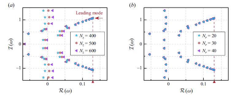
of the disturbance. To this end, we first examined the influence of the number of collocation points,
 $N_z$
and
 $N_r$
, on the eigenvalues
 $\omega$
, as illustrated in figure 9. Owing to numerical discretisations, the eigenvalue spectrum often contains spurious solutions, which generally vary with the resolution of discretisations. Therefore, we mainly focus on the leading mode that should consistently converge to the same value under different
 $N_z$
or
 $N_r$
, and that exhibits the largest temporal growth rate among all the converged eigenvalues (Rubio-Rubio et al. Reference Rubio-Rubio, Sevilla and Gordillo2013; Shukla & Gallaire Reference Shukla and Gallaire2020). As shown in figure 9, the eigenvalue spectra were calculated over the ranges
 $400 \leqslant N_z \leqslant 600$
and
 $20 \leqslant N_r \leqslant 40$
, and the leading mode exhibits excellent convergence. Thus, we set
 $N_z = 400$
and
 $N_r = 20$
in this study.
Verification of mesh independence of the eigenvalue spectrum in the (a) axial and (b) radial directions. The dimensionless numbers were selected to be consistent with figure 5(c), i.e.
 ${\textit{We}} = 1.0$
,
 ${\textit{Re}} = 50$
.

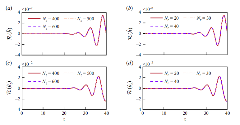
Verification of mesh independence of the eigenfunction corresponding to the leading mode in figure 9. (a,b) Surface displacement disturbance,
 $\mathcal{R}(\hat {h})$
, and (c,d) axial velocity disturbance,
 $\mathcal{R}(\hat {u}_z)$
, along the jet centreline (
 $r = 0$
). Here
 ${\textit{We}} = 1.0$
,
 ${\textit{Re}} = 50$
.

In addition, the convergence of the eigenfunction
 $\hat {\boldsymbol{\phi }}(z,r)$
(i.e. the spatial distribution of the disturbance) associated with the leading mode in figure 9 was also verified, as shown in figure 10. Under different
 $N_z$
or
 $N_r$
, the disturbance profiles almost overlap, verifying the mesh independence of the eigenfunction. For brevity, only representative results are shown here, including the real parts of the surface displacement disturbance,
 $\mathcal{R}(\hat {h})$
, and the axial velocity disturbance at the jet centreline,
 $\mathcal{R}(\hat {u}_z(r=0))$
. It should be noted that the coefficient matrix
 $\boldsymbol{A}$
must first have full rank. Based on this, the eigenfunction should remain identical or linearly related as
 $N_z$
or
 $N_r$
varies. After normalisation, the spatial distribution of each disturbance can then be obtained from the eigenfunction
 $\boldsymbol{\hat {\phi }}$
.
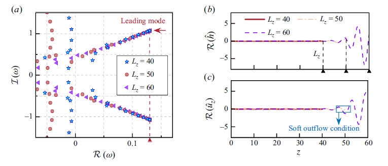
Finally, we examined the influence of the axial computational domain length
 $L_z$
on both the leading eigenvalue and the corresponding eigenfunction, within the range
 $40 \leqslant L_z \leqslant 60$
. As shown in figures 11(b) and 11(c), the disturbance profiles exhibit only minor deviations near the cutoff boundary (
 $z = L_z$
), which can be attributed to the effect of the soft outflow conditions,
 $\hat {u}_{z,z} = \hat {u}_{r,z} = \hat {h}_{,z} = 0$
(Montanero & Gañán-Calvo Reference Montanero and Gañán-Calvo2020). Nevertheless, since the axial domain length is much larger than the jet radius, i.e.
 $L_z \gg 1$
, these slight deviations have no impact on the eigenvalues. Consequently, the leading modes consistently converge to the same value across all cases, as shown in figure 11(a). We thus set
 $L_z = 40$
in this study.
(a) Eigenvalue spectra for different axial computational domain lengths
 $L_z$
, and the corresponding eigenfunctions of the leading modes. (b) Surface displacement disturbance,
 $\mathcal{R}(\hat {h})$
, and (c) axial velocity disturbance,
 $\mathcal{R}(\hat {u}_z)$
, along the jet centreline (
 $r = 0$
). The dimensionless parameters are
 ${\textit{We}} = 1.0$
and
 ${\textit{Re}} = 50$
. The black dotted lines in (b) mark the positions of different cutoff boundaries (
 $z = L_z$
), and the blue box in (c) highlights the minor deviation caused by the soft outflow conditions.