“Come egli è cosa sapientissima simulare in tempo la pazzia.”
[“It is wise to sometimes pretend to be crazy.”]
--Niccolò Machiavelli in Discourses on Livy
In the opening paragraph of his classic article, Fearon (Reference Fearon1995, 379) lists three explanations for the occurrence of wars:
First, one can argue that people (and state leaders in particular) are sometimes or always irrational. They are subject to biases and pathologies that lead them to neglect the costs of war or to misunderstand how their actions will produce it. Second, one can argue that the leaders who order war enjoy its benefits but do not pay the costs, which are suffered by soldiers and citizens. Third, one can argue that even rational leaders who consider the risks and costs of war may end up fighting nonetheless.
Fearon proceeds to focus his attention on the third perspective, which he calls the rationalist explanation of war. Under this perspective, war is an outcome of strategic actions taken by two rational (and unitary) states that have fully considered its costs, benefits and uncertainty.
Indeed, with very few exceptions, the formal literature on war addresses only this rationalist explanation.Footnote 1 Moreover, despite the plausibility of Fearon’s first two explanations, the bulk of this literature makes the idealized assumption that it is common knowledge that all leaders are rational and behave strategically. Yet both historical and contemporary evidence suggests that this assumption is more an idealization of reality rather than a reflection of it.Footnote 2 There is ample evidence that key decision makers have, at various times, tried to build reputations of being crazy or to take advantage of their adversaries’ concerns that they may be irrational. Consider, for example, White House Chief of Staff Bob Haldeman’s (Reference Haldeman1978, 122) recollection of president Richard Nixon explaining to him the ‘madman theory’ at the height of the Vietnam War:
I call it the Madman Theory, Bob. I want the North Vietnamese to believe I’ve reached the point where I might do anything to stop the war. We’ll just slip the word to them that, for God’s sake, you know Nixon is obsessed about communism. We can’t restrain him when he’s angry—and he has his hand on the nuclear button’ and Ho Chi Minh himself will be in Paris in two days begging for peace.
White House papers released in the early 2000s made it clear that the Nixon administration used this madman strategy. On October 10, 1969, Nixon ordered a secret operation called Giant Lance in which 18 B-52 bombers loaded with nuclear weapons flew toward the Soviet Union to get the Soviets to think that he was possibly mad, and that he might be willing to use nuclear weapons in Vietnam (see, for example, Sagan and Suri Reference Sagan and Suri2003).
There is also evidence spanning much of history that other leaders have used the madman strategy, or that they were actually crazy. For example, Kimball (Reference Kimball2004) argues that the Hittite King Mursli used this strategy in antiquity when demanding the release of a hostage. Much more recently, the New York Times reported that in late 2005, US General John Abizaid expressed concern “that Iran’s new President Ahmedinejad seemed unbalanced, crazy even.”Footnote 3 Given the use of the madman strategy in history, and the doubts that contemporary political and military leaders express about the sanity of their adversaries, the idealized assumption of common knowledge of rationality appears at odds with reality.
This article develops a model of war that relaxes the assumption of common (in fact, mutual) knowledge of strategic rationality. Our model builds on the existing crisis bargaining framework, but assumes that there exist types of both countries that have behavioral commitments to particular actions, including how much they are willing to concede in bargaining. In our model, these types are “crazy” in a particular way: whenever they are confronted with a choice between two actions, they always choose the more aggressive one, and at the time of bargaining they only make or accept offers that would give them an unreasonably large payoff. Consequently, one can view our model as bringing together Fearon’s (Reference Fearon1995) three explanations for war. It introduces crazy types who are “subject to biases and pathologies that lead them to neglect the costs of war” or “who enjoy its benefits but do not pay the costs,” and it explores the effect of crazy types on the behavior of the strategically rational types “who [fully] consider the risks and costs… [but] may end up fighting nonetheless.”Footnote 4 More importantly, by introducing crazy types into the standard crisis bargaining model, we are able to analyze the considerations of leaders like Nixon, Abizaid and Ahmedinejad, discussed above, and to assess the effectiveness of the so-called madman theory as a strategy in crisis bargaining.
Our model has three distinctive features. First, despite having two-sided incomplete information, it is tractable and makes (generically) unique equilibrium predictions. In equilibrium, the strategic types of both countries mimic the behavior of the crazy types with positive probability and, as a result, conflict takes place with positive probability (which, of course, is inefficient).
Second, we exploit the uniqueness of our equilibrium predictions to provide new comparative static results relating the probabilities of crazy types, and the countries’ military strengths, to the probability of war. At the heart of these comparative statics are two distinct equilibrium forces that arise due to mutual doubts of strategic rationality: a reputation motive and a defense motive. The reputation motive describes a leader’s incentive to pretend to be crazy in order to get a better settlement, while the defense motive describes a leader’s incentive to make larger demands that risk escalation in order to deter his adversary from pretending to be crazy too often. Our results provide a precise characterization of the combined effect of the reputation and defense motives. This enables us to derive the comparative statics of equilibrium behavior and payoffs with respect to the model’s parameters.
Third, and finally, our article contributes to a long-standing debate about whether the madman strategy ‘works,’ by characterizing the costs and benefits of using this strategy, and the conditions under which it is optimal. We show that these conditions depend largely on prior beliefs—in particular, on the effect that these beliefs have on the balance between the reputation motive for one country and the defense motive for the other. When the prior probability of the crazy type is sufficiently small for each country, both pretend to be crazy with some probability. However, because each country is mixing between escalation and concession, the madman strategy ends up being payoff-neutral. (Pretending to be crazy with a higher probability would result in a lower payoff; committing to pretend with a lower probability would raise payoffs, but would not be credible). This happens because the defense motive pushes a country to adopt more aggressive behavior in order to limit the benefits that its opponent can obtain by also playing aggressively. As the prior probability of the crazy type increases for a particular country, that country puts less probability on the concessional action, and eventually has a strict incentive to pretend to be crazy. Then, the strategy of always pretending to be crazy becomes profitable as the reputation motive is no longer in play (that is, the country no longer seeks to preserve the reputational content of aggressive behavior). Yet when the prior probability with which the other country is crazy exceeds a certain threshold, the madman strategy may not be adopted at all, as the defense motive can no longer compensate for the increase in the expected aggressiveness of the opponent. Therefore, whether or not the madman strategy works depends on prior beliefs about both countries, and on how each country is expected to respond to aggressions. In particular, even if a country has an incentive to occasionally pretend to be crazy, this may be only payoff neutral.
In the remainder of the introduction, we illustrate the most salient features of our approach. Then we review the literature and present the model, along with its comparative statics. The final section concludes.
An Illustration of our Approach
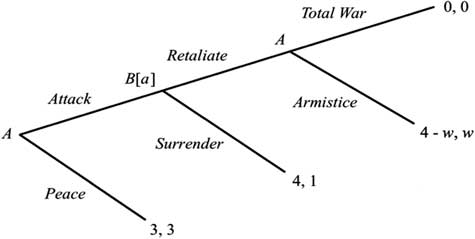
Consider the game tree depicted in Figure
1. Countries A and B are engaged in a dispute. Country A moves
first: the choice is between attacking Country B and resolving the dispute
peacefully. If Country A attacks, then Country B chooses between surrender
and retaliate. If Country B retaliates, then Country A can either end the
war with an armistice or escalate the conflict by choosing total war. Since
all actions are uniquely labeled, we can identify terminal nodes with the
actions that lead to them. We assume that 1<w<3, so
that Country A’s preference over outcomes is Surrender
 $${\succ}_{A} $$
Peace
 $${\succ}_{A} $$
Armistice
 $${\succ}_{A} $$
Total War, while Country B’s preference is Peace
 $${\succ}_{B} $$
Armistice
 $${\succ}_{B} $$
Surrender
 $${\succ}_{B} $$
Total War. Also note that the payoffs in Figure 1 are consistent with the idea
that war is costly: with each aggressive action—attack and retaliate—one
unit of total payoff is lost, and with total war an extra three units are
lost. By backward induction, one can show that under complete information
the unique subgame-perfect equilibrium outcome of the model is peace.
Game tree for the illustrative example

However, suppose that Country B believes that Country A is a strategic type
that plays according to seqential rationality only with probability
 $p\in (0,1)$
; for our purposes, we assume that p is
close to 1. With complementary probability 1−p, Country B
believes that Country A is a crazy type that always chooses attack, and
always chooses total war in the event that Country B chooses to retaliate.
For simplicity, assume that Country A is certain (that is, believes with
probability 1) that Country B is a strategic type that plays according to
sequential rationality. Finally, suppose that these prior beliefs are common
knowledge. It is easy to show that this game has a unique sequential
equilibrium in which the strategic type of Country A attacks Country B with
positive probability, and Country B retaliates with positive probability.
The following is a sketch of the argument.
Sequential rationality requires the strategic type of Country A to always choose armistice over total war when confronted with this decision. Let a denote the equilibrium probability with which Country B believes that Country A is the strategic type, conditional on Country A choosing attack. If Country A attacks, then Country B’s expected payoff from retaliating is aw, while its payoff from surrendering is 1. Consequently, the equilibrium probability with which Country B retaliates is 1 if a>1/w and 0 if a<1/w. Country B mixes between surrender and retaliate only if a=1/w.
Now, it is clear that there is no equilibrium in which the strategic type of Country A chooses peace with probability 1. If there were such an equilibrium, then conditional on Country A choosing to attack, Country B would believe with certainty that Country A is crazy; that is, a=0. But since the crazy type always chooses total war, Country B would surrender for sure. Therefore, the strategic type of Country A would want to deviate to attack. Similarly, there is no equilibrium in which the strategic type of Country A definitely attacks. Otherwise, given that both types of Country A attack, Country B’s posterior would be the same as its prior; that is, a=p. Now, we assumed that p is close to 1; in particular we assume p>1/w. But in this case, Country B retaliates with probability 1, which in turn implies that the strategic type of Country A would want to deviate to peace.
Equilibrium must then involve the strategic type of Country A mixing between
peace and attack, and thus it must be indifferent between these two actions.
This indifference pins down the probability with which Country B retaliates.
It is easy to show that this probability is simply 1/w.
Since Country B mixes between retaliate and surrender, it must be
indifferent between these actions, so
a=1/w. This describes the equilibrium
probability with which the strategic type of Country A chooses to attack:
 $(1{ - }p)/[(w{ - }1)p]> 0$
. This concludes the characterization of
the sequential equilibrium.
Now, define the equilibrium probability of war as the probability that the equilibrium outcome will be armistice or total war:
 $$\mathop{\underbrace{{\left[ {(1{ - }p){\,+\,}{{1{ - }p} \over p} \cdot {1 \over {w{ - }1}}} \right]}}}\limits_{{\rm Pr[A\ attacks]}}{\times}\mathop{\underbrace{{\left[ {{1 \over w}} \right]}}}\limits_{{\rm Pr[B\ retaliates]}}$$
Therefore, the probability with which Country A attacks is increasing in its prior probability of being the crazy type. Also, the probability with which Country A attacks and the probability with which Country B retaliates are both decreasing in w. Since w measures the split of total payoff after an armistice, we conclude that the probability of war is decreasing in the relative strength of Country B.
Equation 1 implies that the equilibrium probability of war goes to 0 as p goes to 1. Nevertheless, even a relatively small probability that Country A is the crazy type can lead to war with significantly higher probability. For example, suppose that w=1.1 so that Country A is relatively stronger than Country B, and there is a 1 percent prior chance that Country A is the crazy type; that is, p=0.99. In this case, the equilibrium probability of war is slightly over 10 percent. This is because the probability with which the strategic type of Country A attacks is slightly above 10 percent, while Country B retaliates with probability slightly larger than 90 percent. Therefore, even a small chance that Country A is crazy may have an amplified effect on its equilibrium behavior. Note also that in this example, slightly over 90 percent of wars are fought between strategic types.
The example above highlights some of the salient features of our approach. However, several questions remain: What happens when both countries have positive prior probability of being crazy? What happens when these probabilities are not as small as we have assumed above? What happens when one country is able to make offers to the other country to avoid war or cease hostilities? In this case, what can one assume about the behavior of the crazy type at the negotiating table? Which incentives determine the probability with which strategic types participate in costly conflicts? Our model addresses all of these questions. It handles two-sided incomplete information with ease, its equilibrium predictions are almost always unique, it generalizes the comparative statics results above, and it identifies the incentives that lie behind them.
Related Literature
Our model builds upon the crisis bargaining literature, which goes back to the work of Powell (Reference Powell1987), Banks (Reference Banks1990) and Fearon (Reference Fearon1995). The chief insight in this literature is that war cannot be an equilibrium outcome when both parties are able to locate a Pareto superior negotiated settlement. By contrast, our model shows that because of the presence of aggressive crazy types, bargaining cannot resolve conflict—even between the strategic types—when they have incentives to pretend to be crazy types that are unreasonably demanding. In this way, our model is most closely related to crisis bargaining models with private information in which the parties involved have incentives to misrepresent their information, for example Fey and Ramsay (Reference Fey and Ramsay2010), Leventoglu and Tarar (Reference Leventoglu and Tarar2008), Slantchev (Reference Slantchev2005) and Schultz (Reference Schultz1999). However, the key difference is that these previous articles incorporate incomplete information by assuming that types can be either ‘tough’ or ‘lenient’ rather than ‘crazy’ or ‘strategic.’ In particular, even the tough types are strategic, and will accept offers that are larger than any payoff they can hope to achieve by rejecting. Besides being qualitatively different, our model facilitates a more tractable analysis and, in contrast to previous articles, yields unique equilibrium predictions, which enables us to deliver a number of comparative statics results relating the probability of war and the payoffs received by the strategic types with the prior probability of the crazy types.
Substantively, our article contributes to the debate about the effectiveness of the madman theory, as articulated by Richard Nixon. Kaplan (Reference Kaplan1991) explains how scholars in the 1950s and 1960s debated the merits of using irrationality and unpredictability in nuclear policy. While some scholars, including Schelling (Reference Schelling1963), did not consider the madman strategy to be effective in the age of nuclear weapons, others, notably Kissinger (Reference Kissinger1969), argued in favor of the madman strategy (claiming that the Soviets were also using it) as well as the merits of limited war (which in our model can be thought of as a war ending with the action we label armistice). Indeed, Kissinger became an ardent supporter of the madman strategy while working for Nixon, and oversaw much of its use in Vietman. For example, Sherry (Reference Sherry1995) argues that the Nixon administration’s decision to indiscriminately bomb Cambodia was a manifestation of the madman theory, while Sagan and Suri (Reference Sagan and Suri2003) recount the use of the madman strategy in Operation Giant Lance, mentioned above. Whether or not the madman strategy works has been debated, however. Jeffrey Kimball writes, for example, that “with or without nuclear threats, the madman theory has worked for some decision makers, leaders, statesmen, tyrants, aggressors, and conquerors during the long course of history, but it has not always worked, and it did not work for Nixon and Kissinger during the Vietman War” (Kimball Reference Kimball2005).
Although the debate over the effectiveness of the madman strategy is yet unresolved, it is possible, and perhaps likely, that the strategy has been used even in contemporary politics. For example, Harvey Simon (Reference Simon2013) suggests that Kim Jong Un might be using the madman strategy, and Lake (Reference Lake2011) writes that the George W. Bush administration thought of Saddam Hussein as “uniquely evil,” suggesting that they might have viewed him as a potential madman. Lake (Reference Lake2011) also advocates a theory of war that accounts for the possibility of cognitive biases and irrationality. As a step in this direction, our model introduces the possibility of a crazy type in the standard crisis bargaining model, and contributes to the debate about the effectiveness of the madman strategy. In particular, we characterize the conditions under which the madman strategy yields a higher expected payoff than any other strategy (making it an equilibrium strategy) and the conditions under which it does not. In doing so, we exploit the uniqueness of equilibrium predictions to derive comparative static results with respect to the aggressiveness of the countries and their relative military strength.
Our article is also closely related to an incisive article by Patty and Weber (Reference Patty and Weber2006), who argue that war cannot arise under the assumption of common knowledge of strategic rationality, but they do not model what happens when this assumption is relaxed. We, on the other hand, explicitly relax the assumption of common knowledge of rationality, and are thus able to characterize the effect of crazy (or, in the language of Patty and Weber, ‘irrational’) types on the equilibrium behavior of strategic types.
Ours is not the first article on international security to study the effect of incorporating behavioral types into an otherwise rational framework. In an early article, Alt, Calvert and Humes (Reference Alt, Calvert and Humes1988) studied deterrence by a hegemonic power against a series of short-run challengers in which the hegemon could possibly be a dominant strategy type as in Kreps and Wilson (Reference Kreps and Wilson1982). These articles, and others in the reputation literature (for example, Fudenberg and Levine Reference Fudenberg and Levine1989), show that the opportunity to build a reputation is payoff improving to the player who takes the opportunity to build it. In contrast to these articles, in our model strategic agents pool with the behavioral type, even though this is (in expectation) payoff-neutral for them. In this way, our article is most closely related to the work of Abreu and Gul (Reference Abreu and Gul2000) on reputational bargaining that shows that a slight possibility of irrationality on either side has a pooling effect that produces inefficient delays in bargaining.Footnote 5
Two compelling foundations for the crazy type that appears in our model emerge from the work of Weisiger (Reference Weisiger2013) in international relations theory, and Bénabou and Tirole (Reference Bénabou and Tirole2009) in behavioral economics. Weisiger (Reference Weisiger2013) argues that uncertainty about leaders’ actual intentions could lead to costly conflict, and generate the belief that some leaders may possess a dispositional inability to commit to peace. Bénabou and Tirole (Reference Bénabou and Tirole2009) study belief distortions created by pride, dignity and wishful thinking about future outcomes, especially as they relate to intransigence in bargaining.
MODEL
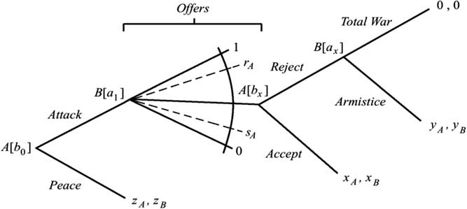
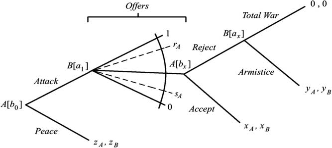
Consider the game tree depicted in Figure
2. Countries A and B are engaged in a dispute. Country A begins by
deciding between peace and attack. In the case of peace, the countries receive
payoffs (z
A
, z
B
). If Country A attacks, then Country B makes an offer
 $$x_{A} \in X\,\equiv\,[0,1]$$
, where x
A
is the payoff it is offering to Country A and
 $$x_{B} \,\equiv\,1{ - }x_{A} $$
is the payoff that it is proposing for itself. Country A can
either accept the offer or escalate the conflict by rejecting it. If it
rejects, then Country B either signs an armistice that leads to payoffs
(y
A
, y
B
), or it chooses total war, which results in payoffs (0, 0). We assume
that war is costly for both sides.
The game tree
Assumption 1. War is costly:
 $$(a)\,z_{A} > y_{A} > 0,\,(b)\,z_{B} > y_{B} > 0,\,{\rm and}\,{\rm (}c{\rm )}\,z_{A} {\,+\,}z_{B} > 1> y_{A} {\,+\,}y_{B} .$$
Under Assumption 1, it is easy to see that with complete information, the game
has a unique subgame perfect equilibrium, the only outcome of which is peace.
However, instead of assuming complete information, suppose that at the
beginning of the game, Country B believes that Country A is strategically
rational only with probability
 $a_{0} \in (0,1)$
; with complementary probability 1−a
0, Country B believes that Country A is a crazy type that always
attacks, and accepts an offer x
A
if and only if
 $$x_{A} \geq r_{A} $$
for some
 $$r_{A} < 1$$
. Similarly, assume that at the beginning of the game Country
A believes that Country B is strategically rational only with probability
 $$b_{0} \in (0,1)$$
; with complementary probability 1−b
0, Country A believes that Country B is a crazy type that always
makes the offer
 $$s_{A} \in X$$
for some
 $$s_{A} {\rm \,>\, }0$$
, and always chooses total war.Footnote
6
We call this game
 $$G(a_{0} ,b_{0} )$$
, and we make the following assumptions on r
A
and s
A
.
Assumption 2. Crazy types are greedy:
 $$(a)\,\,1{ - }y_{B} > r_{A} > z_{A} \ {\rm and}\ (b)\,\,\min \{ 1{ - }z_{B} ,y_{A} \} > s_{A} > 0.$$
Assumption 2a states that the crazy type of Country A seeks a payoff greater than the peaceful payoff z A . It also states that this type is not too demanding: the agreement that it seeks is better for Country B than the outcome under an armistice. This means that Country B has the opportunity to reach a settlement that is better for it than a war that ends in armistice, even when Country A is crazy.Footnote 7 Assumption 2b states that the crazy type of Country B makes an offer that is worse for Country A than the outcome under armistice, and worse than giving Country B the payoff it would have received under peace. Combining Assumptions 1 and 2 yields:
 $$1> r_{A} > y_{A} > s_{A} > 0.$$
It is useful to point out that our assumptions give strategic types the opportunity to prevent either the start or the escalation of a costly war at each node (Country A can choose peace or accept the offer of Country B, while Country B can make the concessional offer r A or choose armistice). We make this modeling choice primarily because we are interested in understanding how the existence of crazy types may lead to costly conflicts between strategic types, even though there are agreements that would be Pareto superior for the strategic types. In other words, we are analyzing a model in which the assumptions are stacked against producing war through the introduction of crazy types.Footnote 8 Nevertheless, we will show that costly wars may take place.
A behavioral strategy profile for the game
G(a
0, b
0) is denoted
 $$\langle (\alpha ,\alpha _{x} ),\,(\beta ,\beta _{{TW}} )\rangle $$
, where α is the probability with which the
strategic type of Country A chooses to attack;
 $$\alpha _{x} :X\to[0,1]$$
is a mapping where
 $$\alpha _{x} (x_{A} )$$
denotes the probability with which the strategic type of
Country A rejects the offer x
A
;
 $$\beta \in \Delta (X)$$
is a probability measure of the set of feasible offers made
by the strategic type of Country B; and
 $$\beta _{{TW}} :X\to[0,1]$$
is a mapping where
 $$\beta _{{TW}} (x_{A} )$$
is the probability with which the strategic type of Country B
chooses total war following the rejection of offer x
A
by Country A. If the strategic types of the two countries play the
behavioral strategy profile
 $$\langle (\alpha ,\alpha _{x} ),(\beta ,\beta _{{TW}} )\rangle $$
, then Country B’s updated belief that Country A is strategic,
conditional on an attack, is:
 $$a_{1} \,\equiv\,{{\alpha a_{0} } \over {1{ - }a_{0} {\,+\,}\alpha a_{0} }}.$$
Country A’s updated belief that Country B is strategic, conditional on
receiving an offer (x
A
, x
B
), is given by the function
 $$b_{x} :X\to[0,1]$$
such that:
 $$b_{x} (x_{A} )=\left\{ {\matrix{ 1 \hfill & {{\rm if}\,x_{A} \,\ne\,s_{A} } \hfill \cr {{{\beta (s_{A} )b_{0} } \over {1{ - }b_{0} {\,+\,}\beta (s_{A} )b_{0} }}} \hfill & {{\rm if}\,x_{A} =s_{A} {\rm .}} \hfill \cr } } \right.$$
We denote Country B’s belief that Country A is strategic at the node at which it chooses between total war and armistice by a x . Although we can characterize a x using Bayes rule, its value will not matter at any information set. This is because Assumption 1b implies that in any perfect equilibrium of the game, the strategic type of Country B will choose armistice.
Definition 1. A sequential equilibrium (or simply equilibrium) of game
 $$G(a_{0} ,b_{0} )$$
is
-
(i) a behavioral strategy profile
 $$\langle (\alpha ,\alpha _{x} ),(\beta ,\beta _{{TW}} )\rangle $$
, and
-
(ii) an associated Bayesian belief system
$$(a_{0} ,a_{1} ,a_{x} ,b_{0} ,b_{x} )$$


such that
 $$(\alpha ,\alpha _{x} )$$
and
 $$(\beta ,\beta _{{TW}} )$$
are sequentially rational given
 $$(a_{0} ,a_{1} ,a_{x} ,b_{0} ,b_{x} )$$
.
Before stating our first proposition, we define the following thresholds:
 $$\underline{a} ={{1{ - }r_{A} { - }y_{B} } \over {1{ - }s_{A} { - }y_{B} }}\quad \quad \bar{a}={{1{ - }r_{A} { - }y_{B} } \over {1{ - }y_{A} { - }y_{B} }}$$
 $$\underline{b} ={{z_{A} { - }s_{A} } \over {r_{A} { - }s_{A} }}\quad \quad \overline{b} ={{s_{A} } \over {y_{A} }}{\,+\,}{{(y_{A} { - }s_{A} )(z_{A} { - }s_{A} )} \over {y_{A} (r_{A} { - }s_{A} )}}.$$
It is easy to verify from Assumptions 1 and 2 that
 $$1> \bar{a}> \underline{a} > 0$$
and
 $$1> \overline{b} > \underline{b} > 0$$
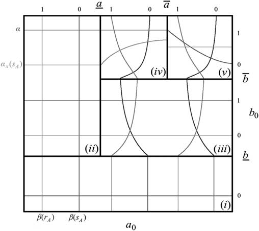
. These thresholds are depicted in Figure 3, which divides the parameter space
 $${\cal P}=(0,1)^{2} $$
into five regions, labeled (i) through
(v). We now characterize the equilibria of the game
G(a
0, b
0) in these five regions, except on the boundaries.Footnote
9
Proposition 1. The equilibria of the game G(a
0, b
0) in Regions (i) to (v) are
characterized as follows. In every equilibrium of the game we have
 $$\beta _{{TW}} (x_{A} )=0$$
for all
 $$x_{A} \in X$$
. Furthermore:
(i) If
 $$b_{0} < \underline{b} $$
, then in every equilibrium, we have
 $$\alpha =0$$
,
 $$\alpha _{x} (x_{A} )\in \left\{ {\matrix{ {\{ 0\} } \hfill & {{\rm if}\,x_{A} =s_{A} \,{\rm or}\,x_{A} > y_{A} } \hfill \cr {\left[ {0,1} \right]} \hfill & {{\rm if}\,x_{A} =y_{A} } \hfill \cr {\{ 1\} } \hfill & {{\rm if}\,x_{A} < y_{A} \,{\rm and}\,x_{A} \,\ne\,s_{A} {\rm ,}} \hfill \cr } } \right.$$
 $$\beta (r_{A} )=1$$
and
 $$\beta (x_{A} )=0$$
for all
 $$x_{A} \,\ne\,r_{A} $$
.
(ii) If
 $$b_{0} > \underline{b} $$
and
 $$a_{0} < \underline{a} $$
, then in every equilibrium, we have
α=1, α
x
is given by (*) above,
 $$\beta (r_{A} )=1$$
and
 $$\beta (x_{A} )=0$$
for all
 $$x_{A} \,\ne\,r_{A} $$
.
(iii) If
 $$\overline{b} > b_{0} > \underline{b} $$
and
 $$a_{0} > \underline{a} $$
, then in every equilibrium, we have
 $$\alpha ={{1{ - }a_{0} } \over {a_{0} }} \cdot {{1{ - }r_{A} { - }y_{B} } \over {r_{A} { - }s_{A} }}$$
, α
x
is given by (*) above,
 $$\beta (s_{A} )=1{ - }{{z_{A} { - }s_{A} } \over {b_{0} (r_{A} { - }s_{A} )}}$$
,
 $$\beta (r_{A} )={{z_{A} { - }s_{A} } \over {b_{0} (r_{A} { - }s_{A} )}}$$
and
 $$\beta (x_{A} )=0$$
for all
 $$x_{A} \,\ne\,s_{A} ,r_{A} $$
.
(iv) If
 $$b_{0} > \overline{b} $$
and
 $$\bar{a}> a_{0} > \underline{a} $$
, then in every equilibrium we have
α=1,
 $$\alpha _{x} (x_{A} )\in \left\{ {\matrix{ {\{ 1\} } \hfill & {{\rm if}\,x_{A} < y_{A} \,{\rm and}\,x_{A} \,\ne\,s_{A} } \hfill \cr {\{ 1{ - }{{1{ - }r_{A} { - }y_{B} } \over {a_{0} (1{ - }s_{A} { - }y_{B} )}}\} } \hfill & {{\rm if}\,x_{A} =s_{A} } \hfill \cr {\left[ {0,1} \right]} \hfill & {{\rm if}\,x_{A} =y_{A} } \hfill \cr {\{ 0\} } \hfill & {{\rm if}\,x_{A} > y_{A} } \hfill \cr } } \right.$$
 $$\ \ \ \beta (s_{A} )={{1{ - }b_{0} } \over {b_{0} }}{{s_{A} } \over {y_{A} { - }s_{A} }}$$
,
 $$\beta (r_{A} )=1{ - }{{1{ - }b_{0} } \over {b_{0} }}{{s_{A} } \over {y_{A} { - }s_{A} }}$$
and
 $$\beta (x_{A} )=0$$
for all
 $$r_{A} \,\ne\,s_{A} ,r_{A} $$
.
(v) If
 $$a_{0} > \bar{a}$$
and
 $$b_{0} > \overline{b} $$
, then in the unique equilibrium
 $$\alpha ={{1{ - }a_{0} } \over {a_{0} }}{{1{ - }r_{A} { - }y_{B} } \over {r_{A} { - }y_{A} }}$$
,
 $$\alpha _{x} (x_{A} )=\left\{ {\matrix{ 1 \hfill & {{\rm if}\,x_{A} < y_{A} \,{\rm and}\,x_{A} \,\ne\,s_{A} } \hfill \cr {{{y_{A} { - }s_{A} } \over {1{ - }s_{A} { - }y_{B} }}} \hfill & {{\rm if}\,x_{A} =s_{A} } \hfill \cr 0 \hfill & {{\rm if}\,x_{A} \geq y_{A} ,} \hfill \cr } } \right.$$
 $$\ \ \ \beta (s_{A} )={{1{ - }b_{0} } \over {b_{0} }}{{s_{A} } \over {y_{A} { - }s_{A} }}$$
,
 $$\beta (y_{A} )=1{ - }{{z_{A} { - }b_{0} y_{A} } \over {b_{0} (r_{A} { - }y_{A} )}}{ - }{{(1{ - }b_{0} )s_{A} } \over {b_{0} (y_{A} { - }s_{A} )}}$$
,
 $$\beta (r_{A} )={{z_{A} { - }b_{0} y_{A} } \over {b_{0} (r_{A} { - }y_{A} )}}$$
and
 $$\beta (x_{A} )=0$$
for all
 $$x_{A} \,\ne\,s_{A} ,y_{A} ,r_{A} $$
.
Proof. See Appendix A.
Equilibrium behavior in the five regions defined in Proposition 1 Note: αx(sA) in orange, β (rA) in blue and β (sA) in brown.
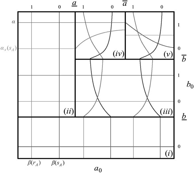
We summarize the main features of equilibrium as follows. If the prior
probability that Country B is strategic is very low,
 $$b_{0} < \underline{b} $$
, then the strategic type of Country A will not attack to
avoid having to bargain with what is likely to be the crazy type of Country B
(Case i). However, the strategic type of Country A may attack when
 $$b_{0} > \underline{b} $$
. If Country A is likely to be crazy,
 $$a_{0} < \underline{a} $$
, while Country B is believed to be strategic with probability
 $$b_{0} > \underline{b} $$
, then the strategic type of Country A will attack for sure,
and the strategic type of Country B will try to settle the dispute early by
making the concessional offer r
A
. This offer will be accepted by both the strategic and crazy types of
Country A (Case ii). If Country A is likely to be strategic,
 $$a_{0} > \underline{a} $$
, and Country B is moderately likely to be strategic,
 $$\overline{b} > b_{0} > \underline{b} $$
, then the strategic type of Country A attacks with
probability
 $$\alpha \in (0,1)$$
. If it attacks, then the strategic type of Country B mixes
between the concessional offer r
A
, which would be accepted for sure, and the greedy offer
s
A
, which the crazy type of Country B would make. Therefore, the strategic
type of Country B sometimes pretends to be crazy (Case iii). This is also what
happens when Country B is very likely to be strategic,
 $$b_{0} > \overline{b} $$
, and Country A is moderately likely to be strategic,
 $$\bar{a}> a_{0} > \underline{a} $$
, except that in this case the strategic type of Country A
attacks for sure (Case iv). Finally, when both countries are very likely to be
strategic,
 $$a_{0} > \bar{a}$$
and
 $$b_{0} > \overline{b} $$
, then Country A mixes between attacking and taking the
peaceful outcome; following an attack, Country B mixes between the
concessional, intermediate and greedy offers, r
A
, y
A
and s
A
(Case v).
An important feature of Proposition 1 is that its predictions are unique. As mentioned above, our model differs from other crisis bargaining models with incomplete information in that it does not lead to multiplicity of equilibrium predictions. The reason for this is as follows. The behavior of the strategic type of each country is determined by two countervailing forces: (1) the incentive to build a reputation for being crazy by mimicking the crazy type and (2) the incentive to deter the opponent from pretending to be crazy too often. For a wide range of values of prior beliefs, a 0 and b 0, equilibrium requires that these two forces exactly offset each other. This can happen only if the strategic type is indifferent between its actions. In turn, this indifference requires that the strategic type assigns a particular probability to its opponent being the crazy type. This probability pins down equilibrium behavior and delivers uniqueness. Put differently, uniqueness stems from the fact that, in equilibrium, the strategic type has to mimic the crazy type with a particular probability, which results in an equilibrium level of reputation that leaves the strategic type of the opponent indifferent between its equilibrium actions.
Furthermore, although Country B has infinitely many possible offers, in equilibrium it only makes one of three offers: a low (greedy) offer s A that corresponds to what the crazy type of Country B would ask for, an intermediate offer y A that is equal to what Country B would offer in the complete information game, and a high (concessional) offer r A that even the crazy type of Country A would accept. Other offers are neither helpful in building a reputation for being crazy, nor optimal against one of the two types of Country A. They reveal that Country B is the strategic type, but conditional on Country A knowing this, Country B could do better.
Also notice that in Region (v) the strategic type of Country B makes offers y A and r A with positive probability, even though both of these offers are accepted with probability 1 by the strategic type of Country A and r A >y A . To understand this feature of equilibrium, notice that these offers yield different payoffs if Country B is facing the crazy type of Country A. Indeed, the crazy type accepts r A and rejects y A with certainty; consequently, Country B’s payoff from making these offers to a crazy type of Country A would be 1−r A and y B , respectively, with 1−r A >y B by Assumption 2a. Proposition 1 implies that the equilibrium-updated belief a 1 will be such that the strategic type of Country B is indifferent between offering r A (and receiving 1−r A with certainty) and offering y A (and receiving 1−y A with probability a 1 and y B with probability 1−a 1).
Finally, Proposition 1 contains the result that uncertainty concerning a country’s type leads to conflict with positive probability, and that conflict is hard to settle. To see this, note that a 0, the probability with which the strategic type of Country A decides to attack, is positive in all regions except (i), and the equilibrium behavior further implies that armistice arises with positive probability in Regions (iv) and (v). Thus not only does the strategic type of Country A initiate conflicts, but the strategic type of Country B may also fail to make offers that would settle them without creating further inefficiency.
We end this section by noting that, as in the illustrative example above, the majority of wars may be fought between strategic types. To see this, define the equilibrium probability of war as the probability with which the game play reaches the node in which Country B must choose between armistice or total war. Then note that the fraction of wars fought between two strategic types is simply:
 $${\rm \,\%}{\rm of}\,{\rm Wars}\,{\rm between}\,{\rm Strategic}\,{\rm Types}={{{\rm Pr[War}\,{\rm between}\,{\rm Strategic}\,{\rm Types]}} \over {{\rm Pr[War]}}}$$
 $$={{\left[ {a_{0} \cdot \alpha \cdot \alpha _{x} (s_{A} )} \right] \cdot \left[ {b_{0} \cdot \beta (s_{A} )} \right]} \over {\left[ {1{ - }a_{0} {\,+\,}a_{0} \cdot \alpha \cdot \alpha _{x} (s_{A} )} \right] \cdot \left[ {1{ - }b_{0} {\,+\,}b_{0} \cdot \beta (s_{A} )} \right]}},$$
where α,
 $$\alpha _{x} (s_{A} )$$
and
 $$\beta (s_{A} )$$
are the equilibrium values of these choice variables given in
Proposition 1. This follows because the unconditional probability that the game
play reaches the node in which Country B chooses between armistice and total
war is the expression in the denominator, while the same probability
(conditional on both types of countries being strategic) is the expression in
the numerator. Then, assume that the payoff parameters of the model are given
by:
 $$z_{A} =z_{B} =0.55,\,\,\,r_{A} =0.555,\,\,\,s_{A} =0.45,\,\,\,y_{A} =0.545,\,\,\,y_{B} =0.1,$$
so that the payoff that a strategic type of Country B can get
from conflict (y
B
) is lower than the payoff that Country A can get (y
A
). Furthermore, let
 $$a_{0} =b_{0} =0.99$$
so that countries are believed to be strategic with 99
percent certainty. In this case, wars fought among strategic types represent
approximately 75 percent of all wars. Thus even though the fraction of crazy
types in the population is relatively small, uncertainty may lead to excessive
aggression by the strategic types, to the point where most wars are fought
among strategic types.
Comparative Statics
In this section we report some of the comparative statics of the model with respect to parameters that have particular interpretations. First we report the comparative statics of equilibrium behavior, and then we report the comparative statics of the ex ante expected payoffs of the strategic types.
Comparative Statics of Equilibrium Behavior
Below, we report the comparative statics of equilibrium behavior with respect to a 0 and b 0, which measure the prevalence of crazy types; with respect to r A and 1−s A , which we interpret as measuring the ‘aggressiveness’ of the crazy types during the bargaining phase of the game; and, finally, with respect to the payoff split from armistice (y A , y B ), which we interpret as reflecting the relative military strength of the two countries during war.
Prevalence of Crazy Types
Proposition 2 below reports the comparative statics of equilibrium behavior (specifically, the choice variables α, α x (x A ) and β(x A)) with respect to a 0 and b 0. (The comparative statics of β TW (x A ) are trivial, since it is always equal to 0). Its proof follows from the equilibrium characterization in Proposition 1, and its visual representation is provided in Figure 3. For ease of reading, we state the result referring to Regions (i) to (v) depicted in the figure, rather than repeating the thresholds that define these regions.
Proposition 2. The comparative statics with respect to a 0 and b 0 are as follows:
-
(1) α is continuous and weakly decreasing in a 0 for all b 0. Furthermore, it is strictly decreasing in a 0 only in Regions (iii) and (v).
-
(2) β(r A ) is constant (and equal to 1) in Regions (i) and (ii), strictly decreasing in b 0 in Regions (iii) and (v) and strictly increasing in b 0 in Region (iv).
-
(3) β(s A ) is constant (and equal to 0) in Regions (i) and (ii), strictly increasing in b 0 in Region (iii) and strictly decreasing in b 0 in Regions (iv) and (v).
-
(4) β(y A ) is constant (and equal to 0) in Regions (i) to (iv) and strictly increasing in Region (v).
-
(5) α x (s A ) is constant (and equal to 0) in Regions (i) to (iii), strictly increasing in a 0 in Region (iv) and constant (strictly between 0 and 1) in Region (v).
Proof. Follows immediately from Proposition 1.
According to Proposition 2, the probability with which the strategic type of Country A attacks is strictly decreasing in Regions (iii) and (v) and constant everywhere else. The intuition for this is similar to the one we provided in the example above. Consider, for instance, Region (v), and recall that Proposition 1 states that Country B mixes between three offers: the concessional offer r A that the crazy type of Country A accepts, the intermediate offer y A and the greedy offer s A . This is possible only if Country B is indifferent between these offers. Now, suppose that a 0 increases while a remains constant. In this case, after an attack, Country B believes that Country A is irrational with lower probability. This, in turn, makes the concessional offer less attractive. So, to keep Country B indifferent between the three offers, the equilibrium value of a must adjust down in order to maintain a fixed posterior probability of Country A being the crazy type. We call this the reputation motive. Intuitively, the reputation motive leads the strategic type of Country A to compensate changes in the exogenous probability of attacking, a 0, with changes in the endogenous probability of attacking, α, in order to maintain a constant level of reputation, a 1. The same intuition holds in Region (iii). In the remaining regions, the incentives for the strategic Country A to mimic the crazy type are either totally absent (Region (i)) or overwhelmingly strong (Regions (ii) and (iv), leading to the result that α is constantly equal to 0 and 1 in these respective cases.
The relationship between β(·) and b 0 is more interesting. Here, there are two competing forces. On the one hand, as we increase b 0, the strategic type of Country B must decrease the probability with which it mimics the crazy type, which is a consequence of a reputation motive analogous to the one we described in the previous paragraph. On the other hand, Country B has to ‘protect’ itself from the possibility of aggressive behavior by Country A. This can be done in two ways: exogenously, by relying on its reputation for being a crazy type, 1−b 0, or endogenously, by decreasing the probability β(r A ) of the concessional offer. In order to prevent the strategic type of Country A from attacking too often, the strategic type of Country B has to substitute an increase in the exogenous parameter b 0 with a decrease in the endogenous probability β(r A ). We call this the defense motive. Obviously, this motive is stronger if there is a high probability that Country A is playing strategically (a 0 high). As a result of these two opposing forces, β(r A ) is increasing in b 0 in Region (iv), where the reputation motive prevails, and decreasing in b 0 in Regions (iii) and (v), where the defense motive prevails. Furthermore, the probability mass lost by offer r A in Country B’s equilibrium strategy as a consequence of the defense motive is reallocated either to the greedy offer s A or to the intermediate offer y A that would arise in the complete information game. In particular, s A receives more of this mass in Region (iii) when the prior probability of Country B being crazy is high, while y A receives more of the mass in Region (v), where this probability is relatively low and it is harder for the strategic type of Country B to mimic the crazy type.
Finally, consider the comparative statics of the probability with which Country A rejects B’s offer, α x (·). Since the strategic type of Country A will always accept offers r A and y A , the only relevant comparative static here is the one of α x (s A ) with respect to a 0. This probability is constantly equal to 0 in Regions (i) to (iii), increasing in a 0 in Region (iv), and equal to a positive constant in Region (v). This happens because at this late node in the game, the reputation motive disappears, but the defense motive is still in play: Country A has to substitute its exogenous reputation with endogenous choices to avoid being exploited. It does this by increasing the probability of rejecting the greedy offer s A .
To sum up, on the one hand, the reputation motive pushes for a decrease in the aggressiveness of strategic types as a result of a decrease in their prior probability of being crazy; on the other hand, because of the defense motive, the strategic types of both countries will react to a decrease in the exogenous probability of being crazy with an increase in the endogenous probability of behaving aggressively.
Aggressiveness of crazy types
The defense motive is also at play when we study how the countries’ probabilities of concession vary as we increase the aggressiveness of the crazy type of the opponent. We measure the aggressiveness of Country A’s crazy type by r A and the aggressiveness of Country B’s crazy type by 1−s A . (Here, we identify aggressiveness as the minimum share of surplus that the crazy type seeks during the bargaining part of the game.) As we increase r A , the probability β (r A ) with which the strategic type of Country B makes the concessional offer decreases. Similarly, as we decrease s A , the probability α x (s A ) with which the strategic type of Country A rejects the greedy offer s A goes up. The intuition for these results is that in both of these cases, the defense motive pushes strategic types to react to an exogenous increase in the aggressiveness of the opponent by lowering the probability with which they submit to aggressive behavior. This result is summarized in the following proposition.
Proposition 3. In equilibrium:
-
(1) The probability β (r A ) with which Country B makes the concessional offer is weakly decreasing in r A .
-
(2) The probability α x (s A ) with which Country A rejects the greedy offer of Country B is weakly decreasing in s A .
Proof. See Appendix B.
Military strength
We now consider the comparative statics of equilibrium behavior with respect to changes in y A while holding the sum y A +y B constant. We are interested in these comparative statics because we interpret the payoff split (y A, y B ) as a measure of the relative military strength of the two countries. The stronger a country is, the larger the share of payoffs it can expect to receive following a war that ends in armistice. To state the result of this section, we make the following assumption:
Assumption 3.
 $$h=(z_{A} ,z_{B} ,s_{A} ,r_{A} ,y_{A} ,y_{B} )$$
and
 $$h'=(z_{A} ,z_{B} ,s_{A} ,r_{A} ,y'_{A} ,y'_{B} )$$
are payoff profiles, each satisfying Assumptions
1 and 2. Furthermore,
 $$y_{A} {\,+\,}y_{B} =y'_{A} {\,+\,}y'_{B} =\bar{y}$$
, and
 $$y'_{A} > y_{A} $$
.
Our objective is to study the effect of a change from payoff profile
h to
 $$h'$$
on the equilibrium behavior characterized in
Proposition 1. Let α, α
x
and β denote the equilibrium quantities evaluated
at payoff profile h, and let
 $$\alpha '$$
,
 $$\alpha '_{x} $$
and
 $$\beta '$$
denote the same quantities evaluated at payoff profile
 $$h'$$
. Similarly,
 $$\bar{a}$$
,
 $$\underline{a} $$
,
 $$\bar{b}$$
and
 $$\underline{b} $$
are the thresholds in Part 5 evaluated at
h, while
 $$\bar{a'}$$
,
 $$\underline{a} '$$
,
 $$\bar{b'}$$
and
 $$\underline{b} '$$
are the thresholds evaluated at
 $$h'$$
. It is straightforward to verify the following
(in)equalities:
 $$\underline{a} '> \underline{a} ,\,\,\,\bar{a'}> \bar{a},\,\,\,\underline {b}=\underline {b}',\,\,\,\bar{b'}< \bar{b}.$$
Now, define
 $$\tilde{a}=\left( {{{1{ - }s_{A} { - }y_{B} } \over {1{ - }s_{A} { - }y'_{B} }}} \right)\bar{a'}.$$
One can verify that
 $$\tilde{a}\in (\bar{a},\bar{a'}')$$
. Given this, the following proposition characterizes
the comparative statics of the equilibrium behavior with respect to the
payoff split (y
A,
y
A
).Footnote
10
Proposition 4. The following are true:
-
(1) If
$$a_{0} < \underline{a} $$
or if
$$b_{0} < \underline{b} $$
or if
$$a_{0} \in (\underline{a} ,\bar{a})$$
and
$$b_{0} > \overline{b} $$
, then
$$\alpha '=\alpha $$
; otherwise,
$$\alpha '> \alpha $$
. -
(2) If
$$a_{0} < \underline{a} $$
or if
$$b_{0} < \underline{b} $$
or if
$$a_{0} > \underline{a} '$$
and
$$b_{0} \in (\underline{b} ,\bar{b'})$$
, then
$$\beta '(s_{A} )=\beta (s_{A} )$$
; otherwise,
$$\beta '(s_{A} )< \beta (s_{A} )$$
. -
(3) If
$$a_{0} < \underline{a} $$
or if
$$b_{0} < \underline{b} $$
or if
$$a_{0} > \underline{a} $$
and
$$b_{0} \in (\underline{b} ,\bar{b'})$$
, then
$$\beta '(r_{A} )=\beta (r_{A} )$$
; if
$$a_{0} > \bar{a'}$$
and
$$b_{0} > \bar{b'}$$
then
$$\beta '(r_{A} )< \beta (r_{A} )$$
; otherwise,
$$\beta '(r_{A} )> \beta (r_{A} )$$
. -
(4) If
$$a_{0} > \bar{a'}$$
and
$$b_{0} > \bar{b'}$$
then
$$\beta '(y_{A} )> \beta (y_{A} )$$
; if
$$a_{0} \in (\bar{a},\bar{a'})$$
and
$$b_{0} > \overline{b} $$
then
$$\beta '(y_{A} )< \beta (y_{A} )$$
; otherwise,
$$\beta '(y_{A} )=\beta (y_{A} )$$
. -
(5) If
$$a_{0} > \underline{a} '$$
and
$$b_{0} \in (\bar{b'},\bar{b})$$
or if
$$a_{0} \in (\tilde{a},1)$$
and
$$b_{0} > \bar{b}$$
then
$$\alpha '_{x} (s_{A} )> \alpha _{x} (s_{A} )$$
; if
$$a_{0} \in (\underline{a} ,\tilde{a})$$
and
$$b_{0} > \bar{b}$$
then
$$\alpha _{{x'}} (s_{A} )< \alpha _{x} (s_{A} )$$
; otherwise,
$$\alpha '_{x} (s_{A} )=\alpha _{x} (s_{A} )$$
.


Proof. See Appendix C.
The proof of the proposition in Appendix C utilizes the fact that a
discrete change in y
A
keeping
 $$\bar{y}$$
fixed has two effects. First, it modifies the
boundaries of four out of the five regions defined in Proposition 1.
Second, it affects the equilibrium behavior of countries within each of
the five new regions. The comparative statics of the equilibrium behavior
must take into account the combination of these two effects, since
equilibrium strategies may differ across the boundaries of the five
regions.
The result of Proposition 4 can be understood as follows. Part 1 of the
proposition states the intuitive result that an increase in the relative
military strength of Country A makes it behave (weakly) more
aggressively. In particular, the probability of an attack increases
unless Country A was attacking either with probability 1 or with
probability 0; in the latter case, Country B’s reputation for being crazy
is so high that it discourages Country A from initiating a conflict. Part
2 states that the probability of making the greedy offer weakly decreases
with Country A’s relative military strength, because an increase in
y
A
reduces Country B’s equilibrium expected payoff from mimicking the
crazy type. (Recall that an increase in y
A
is compensated by a decrease in y
B
.) Part 3 states that an increase in Country A’s relative military
strength has an ambiguous effect on the equilibrium probability with
which Country B makes the concessional offer. Intuitively, an increase in
y
A
has two effects. First, for the same reason as before, it makes
the concessional offer more appealing for Country B. Second, by
increasing the expected payoff from attacking, it makes the strategic
type of Country A more aggressive. Thus due to the defense motive
described above, the strategic type of Country B must decrease the
probability of concession. Depending on which of these forces prevails,
the probability of making the concessional offer could either increase or
decrease. Similar reasoning lies behind the intuition of Part 4, which
states that an increase in the relative military strength of Country A
has an ambiguous effect on the probability with which Country B makes the
intermediate offer y
A
. (Note that
 $$\beta (y_{A} )=1{ - }\beta (s_{A} ){ - }\beta (r_{A} )$$
). Finally, Part 5 states that the effect of an increase
in the military strength of Country A has an ambiguous effect on whether
Country A accepts or rejects Country B’s greedy offer. Once more, the
reason for this is that the defense motive for Country A serves as a
countervailing force vis-à-vis the increase in expected payoff associated
with the rejection of the greedy offer.
Therefore, due to the defensive motive, an increase in the military
strength of Country A may lead Country B to be less accommodating and to
test Country A’s true type by making the intermediate offer
y
A
. Notice that this result holds when there is little uncertainty
that Country A is strategically rational; that is, when
 $$a> \bar{a'}$$
. This is exactly the parameter range in which the
strategic type of Country B is more concerned about defending itself
against attacks from the strategic type of Country A.
Comparative Statics of Equilibrium Payoffs
In this section, we study the comparative statics of ex ante expected payoffs with respect to the prevalence and aggressiveness of crazy types in our model. Proposition 1 immediately implies that Country A’s ex ante expected payoff is equal to
 $$V_{A} =\left\{ {\matrix{ {z_{A} } \hfill & {{\rm in\ regions}\,{\rm (i),}\,{\rm (iii),}\,{\rm (v)}} \hfill \cr {b_{0} r_{A} {\,+\,}(1{ - }b_{0} )s_{A} } \hfill & {{\rm in\ region}\,{\rm (ii)}} \hfill \cr {b_{0} \beta (r_{A} )r_{A} {\,+\,}[1{ - }b_{0} \beta (r_{A} )]s_{A} } \hfill & {{\rm in\ region}\,{\rm (iv)}} \hfill \cr } }, \right.$$
where the equilibrium value of β (r A ) in Region (iv) is given in Proposition 1. Furthermore, since Proposition 1 says that Country B always puts positive probability on offer r A , Country B’s expected payoff at the node at which it makes an offer is always 1−r A . This implies that Country B’s ex ante expected payoff is always given by
 $$\eqalignno{ V_{B} =&\,a_{0} [(1{ - }\alpha )z_{B} {\,+\,}\alpha (1{ - }r_{A} )]{\,+\,}(1{ - }a_{0} )(1{ - }r_{A} ) \cr =&\,z_{B} { - }(1{ - }a_{0} {\,+\,}a_{0} \alpha )[z_{B} { - }(1{ - }r_{A} )] $$
where α takes its equilibrium value in
Proposition 1 depending on which of the five regions the parameters
 $$(a_{0} ,b_{0} )$$
fall in. Thus Country B’s expected payoff is always
strictly less than z
B
since
 $$z_{B} > 1{ - }r_{A} $$
, which follows from Assumptions 1c and 2a.
Prevalence of crazy types
It is straightforward to verify that V
A
is larger than z
A
in Regions (ii) and (iv).
Therefore, recalling that
 $$r_{A} > z_{A} > s_{A} $$
, we know that Country A’s payoff is always weakly
decreasing in the prior probability that Country B is the crazy type,
1−b
0, and strictly decreasing in Regions (ii)
and (iv). The reason for this is that a higher
probability of facing the crazy type reduces Country A’s incentive to
play aggressively. Yet Country A’s payoff is piecewise constant in
1−a
0, with upward jumps when a
0 crosses
 $$\bar{a}$$
and
 $$\underline{a} $$
in the region where
 $$b_{0} > \underline{b} $$
. Indeed, if its own prior reputation for being crazy
exceeds a critical value, Country A will be able to ignore the reputation
motive and adjust its equilibrium behavior in order to obtain a higher
payoff.
For similar reasons, V B is always decreasing in the prior probability, 1−a 0, with which its opponent is crazy, and strictly decreasing in Regions (i), (iii) and (v). Furthermore, it is piecewise constant in 1–b 0 with discrete upward jumps when b 0 crosses the boundaries of the equilibrium regions. We summarize the above discussion as follows.
Proposition 5.
-
(1) Country A’s ex ante expected payoff V A is:
-
(a) weakly increasing in b 0 and strictly increasing in Regions (ii) and (iv).
-
(b) piecewise constant in a 0 with downward jumps at the boundaries of Regions (ii), (iii), (iv) and (v).
-
(2) Country B’s ex ante expected payoff V B is:
-
(a) weakly increasing in a 0 and strictly increasing in Regions (i), (iii) and (v).
-
(b) piecewise constant in b 0 with downward jumps at the region boundaries.
Proof. Follows from the characterization of Proposition 1.
Aggressiveness of crazy types
Unlike the comparative statics of payoffs with respect to the prevalence of crazy types, the comparative statics of payoffs with respect to the aggressiveness of crazy types may be ambiguous. The reason behind this ambiguity hinges on the joint effect of the reputation and defense motives.
First, consider Country A. Changes in r
A
and 1−s
A
affect equilibrium behavior both because these changes may affect
behavior within the various regions and because they may affect the
boundaries of these regions. As a result, V
A
will sometimes be increasing, sometimes be decreasing and
sometimes remain constant in r
A
and s
A
. Indeed, as r
A
increases, the strategic type of Country A gains more from
mimicking the crazy type. Thus, keeping equilibrium behavior constant, a
rise in r
A
would increase Country A’s payoff. However, due to the reputation
motive for Country A, the strategic type of Country A will have to lower
its probability of attacking in order to preserve its reputation.
Furthermore, due to the defense motive of Country B, the probability with
which the strategic type of Country B makes the concessional offer has to
decrease. Since these two forces result in a decrease in
V
A
, the ex ante payoff of Country A may end up being
constant or decreasing in r
A
. Yet as s
A
decreases (so that
 $$1{ - }s_{A} $$
increases), mimicking the crazy type becomes less
profitable for the strategic type of Country A and more profitable for
the strategic type of Country B. As a result, the reputation motives of
both countries may result in an increase in α and a
decrease in β (s
A
); when these effects are particularly strong (as is the case in
Region (iv)), V
A
may increase the aggressiveness of Country B’s crazy type.
Now, consider Country B. The ex ante payoff of the
strategic type of Country B varies ambiguously with r
A
, because a rise in r
A
has two opposing effects. On the one hand, it decreases the payoff
that Country B can get by making the concessional offer and,
consequently, lowers its expected payoff. On the other hand, because of
Country A’s reputation motive, it lowers the probability,
α, of an attack, which has the effect of increasing
Country B’s payoff. Depending on which effect dominates,
V
B
could either decrease or increase in r
A
. Finally, a change in the aggressiveness of Country B’s crazy
type,
 $$1{ - }s_{A} $$
, can also have ambiguous effects on V
B
through its effect on α. Once more, this is the
result of two countervailing forces. First, a decrease in
s
A
directly lowers α, as it decreases the payoff
that the strategic type of Country A can get from mimicking the crazy
type. Second, for similar reasons as before, it relaxes the constraints
of the reputation motive, and pushes for an increase in
α.
The characterization of these comparative statics results follows almost
immediately from Proposition 1, but the formal statement of our result,
which we present next, requires us to take into account the effects of
changes in r
A
or s
A
in several regions of the parameter space. To that end, let
 $$h=(z_{A} ,z_{B} ,s_{A} ,r_{A} ,y_{A} ,y_{B} )$$
,
 $$h^{{\ast}} =(z_{A} ,z_{B} ,s_{A} ,r'_{A} ,y_{A} ,y_{B} )$$
and
 $$h^{\dag } =(z_{A} ,z_{B} ,s'_{A} ,r_{A} ,y_{A} ,y_{B} )$$
be three parameter profiles, each satisfying
Assumptions 1 and 2, and assume that
 $$r'_{A} > r_{A} $$
and
 $$s_{A} > s'_{A} $$
. Let
 $$\underline{a} $$
,
 $$\bar{a}$$
,
 $$\underline{b} $$
and
 $$\overline{b} $$
define the boundaries of the regions at profile
h;
 $$\underline{a} ^{{\ast}} $$
,
 $$\bar{a}^{{\ast}} $$
,
 $$\underline{b} ^{{\ast}} $$
and
 $$\bar{b}^{{\ast}} $$
define the boundaries at profile
 $$h^{{\ast}} $$
; and
 $$\underline{a} ^{\dag } $$
,
 $$\overline{a} ^{\dag } $$
,
 $$\underline{b} ^{\dag } $$
and
 $$\overline{b} ^{\dag } $$
define the boundaries at profile
 $$h^{\dag } $$
. Similarly, let V
A
and V
B
be the ex ante expected payoffs under
h;
 $$V_{A}^{{\ast}} $$
and
 $$V_{B}^{{\ast}} $$
be the same payoffs under
 $$h^{{\ast}} $$
; and
 $$V_{A}^{\dag } $$
and
 $$V_{B}^{\dag } $$
be the same payoffs under
 $$h^{\dag } $$
. We then have the following result:
Proposition 6. Country A’s payoffs satisfy
 $$V_{A}^{{\ast}} \left\{ {\matrix{ {>\!V_{A} } \hfill & {{\rm if}\,a_{{\rm 0}} \leq \underline{a} ^{{\ast}} \,{\rm and}\,b_{{\rm 0}} \geq \underline{b} ^{{\rm {\ast}}} {\rm ;or}\,{\rm if}\,a_{{\rm 0}} \in {\rm [}\underline{a} {\rm ,}\bar{a}^{{\rm {\ast}}} {\rm ]}\,{\rm and}\,b_{{\rm 0}} \geq \overline{b} {{{^\ast}}} } \hfill \cr {< \!V_{A} } \hfill & {{\rm if}\,a_{{\rm 0}} \in {\rm [}\underline{a} ^{{\rm {\ast}}} {\rm ,}\underline{a} {\rm ]}\,{\rm and}\,b_{{\rm 0}} \geq \underline{b} {\rm ;or}\,{\rm if}\,a_{{\rm 0}} \in {\rm [}\bar{a}^{{\rm {\ast}}} {\rm ,}\bar{a}{\rm ]}\,{\rm and}\,b_{{\rm 0}} \geq \bar{b}} \hfill \cr {=\!V_{A} } \hfill & {{\rm elsewhere}} \hfill \cr } } \right.$$
 $$\!\!\!\!\!\!\!\!\!\!\!\!V_{A}^{\dag } \left\{ {\matrix{ {< \!V_{A} } \hfill & {{\rm if}\,a_{{\rm 0}} \leq \underline{a} \,{\rm and}\,b_{{\rm 0}} \geq \underline{b} {\rm ;}\,{\rm or}\,{\rm if}\,a_{{\rm 0}} \in {\rm [}\underline{a} {\rm ,}\bar{a}{\rm ]}\,{\rm and}\,b_{{\rm 0}} \geq \bar{b}} \hfill \cr {> \!V_{A} } \hfill & {{\rm if}\,a_{{\rm 0}} \in {\rm [}\underline{a} {\rm ,}\bar{a}{\rm ]}\,{\rm and}\,b_{{\rm 0}} \in {\rm [}\overline{b} ^{\dag } {\rm ,}\bar{b}{\rm ]}} \hfill \cr {=\!V_{A} } \hfill & {{\rm elsewhere}} \hfill \cr } }. \right.$$
For some threshold
 $$\bar{z}> 0$$
(derived in Appendix D), Country B’s payoffs
satisfy
 $$V_{B}^{{\ast}} \left\{ {\matrix{ {> \!V_{B} } \hfill & {{\rm if}\,a_{0} \in [\underline{a} ^{{\ast}} ,\underline{a} ]\,{\rm and}\,b_{0} \in [\underline{b} ,\overline{b} {{^\ast}} ];\,{\rm or}\,{\rm if}\,a_{0} \in [\bar{a}^{{\ast}} ,\bar{a}]\,{\rm and}\,b_{0} \geq \overline{b} ,} \hfill \cr {} \hfill & {{\rm or}\,{\rm if}\,z_{B} > 1{ - }y_{A} ,a_{0} \geq \bar{a}\,{\rm and}\,b_{0} \geq \bar{b};\,{\rm or}\,{\rm if}\,z_{B} > \bar{z},a_{0} \geq \bar{a}^{{\ast}} \,{\rm and}\,b_{0} \in [\bar{b}^{{\ast}} ,\bar{b}]} \hfill \cr {< \!V_{B} } \hfill & {{\rm if}\,a_{0} \in [\underline{a} ^{{\ast}} ,\underline{a} ]\,{\rm and}\,b_{0} \in [\underline{b} ,\,\bar{b}^{{\ast}} ];{\rm or}\,a_{0} \in [\bar{a}^{{\ast}} ,\bar{a}]\,{\rm and}\,b_{0} \geq \bar{b};} \hfill \cr {} \hfill & {{\rm or}\,{\rm if}\,z_{B} > 1{ - }y_{A} ,a_{0} \geq \bar{a}\,{\rm and}\,b_{0} \geq \bar{b};\,{\rm or}\,if\,z_{B} > \bar{z},\,a_{0} \geq \bar{a}^{{\ast}} \,{\rm and}\,b_{0} \in [\bar{b}^{{\ast}} ,\bar{b}]} \hfill \cr {=\!V_{B} } \hfill & {{\rm elsewhere}} \hfill \cr } } \right.$$
 $$V_{B}^{\dag } \left\{ {\matrix{ {< \!V_{B} } \hfill & {{\rm if}\,a_{{\rm 0}} > \underline{a} \,{\rm and}\,b_{{\rm 0}} \in {\rm [}\overline{b} ^{\dag } {\rm ,}\overline{b} {\rm ]}} \hfill \cr {> \!V_{B} } \hfill & {{\rm if}\,b_{{\rm 0}} \in {\rm [}\underline{b} {\rm ,}\,\underline{b} ^{\dag } {\rm ];or}\,{\rm if}\,a_{{\rm 0}} > \underline{a} ^{\dag } \,{\rm and}\,b_{{\rm 0}} \in {\rm [}\underline{b} ^{\dag } {\rm ,}\,\overline{b} ^{\dag } {\rm ]}} \hfill \cr {=\!V_{B} } \hfill & {{\rm elsewhere}} \hfill \cr } }. \right.$$
Proof. See Appendix D.
Final Remarks
We constructed a model of international conflict in which war arises as a result of uncertainty about whether countries behave strategically. This uncertainty may lead even strategic countries to behave according to Machiavelli’s dictum that “it is sometimes wise to pretend to be crazy.” By characterizing the exact conditions under which this happens, the article contributes to a long-standing debate in the literature about the effectiveness of the so-called madman strategy, which has been used by leaders throughout history.
Unlike the previous literature, our model delivers unique equilibrium predictions, which enable us to derive a number of new, but natural, comparative static results. In particular, our model identifies two countervailing effects that play a role in determining how often countries pretend to be crazy: the reputation motive and the defense motive. Whereas the defense motive provides a country with incentives to behave aggressively (to shield itself from aggression by the opponent), the reputation motive limits the extent to which a country can pretend to be crazy. Depending on which of these two forces prevails, conflict may arise and persist, exacerbating the inefficiencies associated with war.
Furthermore, we show how the balance between the reputation and defense motives is essential in determining the profitability of the madman strategy. Indeed, a country’s incentives to pretend to be crazy are limited both by its own reputation motive and by the defense motive of the other country. Thus changes in leaders’ perceived aggressiveness (measured in our model either by the prevalence or intransigence of their crazy types) may have ambiguous and non-obvious effects on the probability of conflict.
One of the peculiar features of the model is the treatment of the two countries
as being asymmetric, in the sense that Country A is a first mover and can
unilaterally impose peace on Country B. This assumption is built into the game
form. Given this rigidity, the most natural way to interpret the model is to
assume that Country A, the first mover, is possibly dissatisfied with the
status quo and may seek to change it with force. Country B, on the other hand,
is not dissatisfied, but has to entertain the possibility that Country A may
use force. One simple remedy for this extreme asymmetry is to assume that there
are two countries, say P and Q, which are
chosen with equal probability to play the game in the role of Country A with
the other country playing in the role of Country B. This is the case of extreme
symmetry. More generally, one could assume that P is chosen to
play in the role of Country A with some probability
 $${\tf="Pi2"\char"6c} \in [0,1]$$
while Q is chosen to play in the role of
Country A with complementary probability
 $$1{ - }{\tf="Pi2"\char"6c} $$
. In this case, all actions, payoffs and comparative statics
(that is, derivatives of equilibrium actions and payoffs) for each country
would be weighted by λ and
 $$1{ - }{\tf="Pi2"\char"6c} $$
.
Finally, by assuming that the crazy type of Country A always accepts offers that are at least as large as r A , and by assuming that the bargaining stage of the game is a static interaction, we are ruling out the possibility that crazy types can keep coming back to demand more each time they are appeased. An interesting extension to the model would be to introduce the possibility that crazy types become more demanding whenever their current demands are met. To analyze this extension, we would need to first develop a dynamic model, and then model the crazy type in this way. We think this would be a fruitful avenue of future research. Nevertheless, the current article is a first step toward relaxing the strong common-knowledge-of-rationality assumptions that pervade crisis bargaining theory.
Appendix
A. Proof of Proposition 1
For any belief a
x
, sequential rationality requires
 $$\beta _{{TW}} (x_{A} )=0$$
. The remaining assertions of the proposition are an
immediate consequence of the following lemmata. The first three are
preliminary results. The latter five each characterize the equilibria in
one of the five regions of the parameter space.
Lemma 1:
(i) In any equilibrium of the game, we have
 $$\alpha _{x} (x_{A} )\in \left\{ {\matrix{ {\{ 0\} } \hfill & {{\rm if}\,b_{x} < x_{A} {\rm /}y_{A} } \hfill \cr {\left[ {0,1} \right]} \hfill & {{\rm if}\,b_{x} =x_{A} {\rm /}y_{A} } \hfill \cr {\{ 1\} } \hfill & {{\rm if}\,b_{x} > x_{A} {\rm /}y_{A} {\rm .}} \hfill \cr } } \right.$$
Consequently, the strategic Country A must accept any
offer
 $$x_{A} > y_{A} $$
.
(ii) If
 $$\beta (s_{A} )=0$$
in equilibrium, then
 $$\alpha _{x} (x_{A} )\in \left\{ {\matrix{ {\{ 0\} } \hfill & {{\rm if}\,x_{A} =s_{A} \,{\rm or}\,x_{A} > y_{A} } \hfill \cr {\left[ {0,1} \right]} \hfill & {{\rm if}\,x_{A} =y_{A} } \hfill \cr {\{ 1\} } \hfill & {{\rm if}\,x_{A} < y_{A} \,{\rm and}\,x_{A} \,\ne\,s_{A} {\rm ;}} \hfill \cr } } \right.$$
(iii) If in equilibrium
 $$\alpha =0$$
, then
 $$\beta (r_{A} )=1$$
.
(iv) If in equilibrium
 $$\beta (y_{A} )> 0$$
, then
 $$\alpha _{x} (y_{A} )=0$$
.
Proof.
-
(i) At the node labeled
$$A[b_{x} ]$$
, rejecting the offer
$$(x_{A} )$$
gives the strategic Country A a payoff of
y
A
with probability b
x
and 0 with probability
$$1{ - }b_{x} $$
. On the other hand, accepting produces a
payoff of x
A
for sure. Therefore, it accepts for sure if
$$b_{x} < x_{A} /y_{A} $$
, rejects for sure if
$$b_{x} > x_{A} /y_{A} $$
, and is indifferent between accepting and
rejecting if
$$b_{x} =x_{A} /y_{A} $$
. Since it must always be that
$$b_{x} \in [0,1]$$
, Country A will accept any offer
$$x_{A} > y_{A} $$
. -
(ii) Observe that if
$$\beta (s_{A} )=0$$
then from Equation 4 in the main
text,(A2)This, along with (A1), immediately gives (*).
$$b_{x} (x_{A} )=\left\{ {\matrix{ 1 \hfill & {{\rm if}\,x_{A} \,\ne\,s_{A} {\rm .}} \hfill \cr 0 \hfill & {{\rm if}\,x_{A} =s_{A} } \hfill \cr } } \right.$$
-
(iii) If
$$\alpha =0$$
, then
$$a_{1} =0$$
. Therefore, Country B believes that Country A
will reject any offer
$$x_{A} < r_{A} $$
. So by making such an offer it expects to
receive a payoff of y
B
. On the other hand, the offer r
A
would be accepted for sure and give Country B a payoff of
$$1{ - }r_{A} > y_{B} $$
. Therefore, the strategic Country B will make
offer the offer r
A
with certainty. -
(iv) By the result of (iii), if Country B makes the offer y A with positive probability, then it must be that
$$\alpha > 0$$
, consequently
$$a_{1} > 0$$
. Suppose, for the sake of contradiction, that
the strategic Country A rejects this offer with probability
$$\delta > 0$$
. Then the expected payoff to Country B of
making this offer is


 $$a_{1} (\delta y_{B} {\,+\,}(1{ - }\delta )(1{ - }y_{A} )){\,+\,}(1{ - }a_{1} )y_{B} .$$
But by making the offer
 $$y_{A} {\,+\,}{\varepsilon}$$
, where
 $$0< {\varepsilon}< \delta (1{ - }y_{A} { - }y_{B} )$$
, Country B would have an expected payoff
of
 $$a_{1} (1{ - }y_{A} { - }{\varepsilon}){\,+\,}(1{ - }a_{1} )y_{B} ,$$
since by Lemma 1(i) the offer
 $$y_{A} {\,+\,}{\varepsilon}$$
is accepted by the strategic Country A. One can then
use the assumption that
 $${\varepsilon}< \delta (1{ - }y_{A} { - }y_{B} )$$
to verify that the payoff in Inequality A4 is greater
than the payoff in Inequality A3.
Lemma 2: In any equilibrium of the game, the support of β
is a subset of the following set of three offers:
 $$\{ s_{A} ,y_{A} ,r_{A} \} $$
.
Proof. Recall that Equation 19 in the main text states that
 $$1> r_{A} > y_{A} > s_{A} > 0$$
. So what we must show is that β does
not put any probability mass on the intervals
 $$[0,s_{A} )$$
,
 $$(s_{A} ,y_{A} )$$
,
 $$(y_{A} ,r_{A} )$$
and
 $$(r_{A} ,1]$$
. Next, observe that if
 $$a_{1} =0$$
, then
 $$\alpha =0$$
and by Lemma 1(iii), only
r
A
is in support of β. Therefore, we can assume
throughout the remainder of this proof that
 $$a_{1} > 0$$
.
Suppose β puts positive mass on
 $$(r_{A} ,1]$$
. By Lemma 1(i), any offer
 $$x_{A} \in (r_{A} ,1]$$
will be accepted by both the strategic type and the
crazy type; so it will be accepted with certainty. But so will the offer
r
A
. Since
 $$1{ - }r_{A} > 1{ - }x_{A} $$
for all
 $$x_{A} \in (r_{A} ,1]$$
, Country B has a profitable deviation to the offer
r
A
. Therefore, β must put zero probability mass on
 $$(r_{A} ,1]$$
.
Suppose that β puts positive mass on
 $$(y_{A} ,r_{A} )$$
. Then, there exists
 $$x_{A} \in (y_{A} ,r_{A} )$$
in support of β. If such an offer
x
A
is made, then by Lemma 1(i) it is accepted with
probability a
1 and rejected with probability
 $$1{ - }a_{1} $$
. But again by Lemma 1(i), the offer
 $${{x_{A} {\,+\,}y_{A} } \over 2}$$
will also be accepted with probability
a
1 and rejected with probability
 $$1{ - }a_{1} $$
. Moreover, deviating to this offer is profitable for
Country B. Therefore it cannot be that x
A
is in support of β. Consequently,
β cannot put positive probability on the interval
 $$(y_{A} ,r_{A} )$$
.
Now suppose that β puts positive mass on
 $$[0,s_{A} ){\cup}(s_{A} ,y_{A} )$$
. Then if Country B makes an offer
 $$x_{A} \in [0,s_{A} ){\cup}(s_{A} ,y_{A} )$$
, we have
 $$b_{x} (x_{A} )=1$$
by Equation 4 in the main text. Therefore, Country B’s
expected payoff of making the offer x
A
is equal to y
B
. But if Country B deviates to the offer
 $$y_{A} {\,+\,}{\varepsilon}$$
, where
 $$0< {\varepsilon}< 1{ - }y_{A} { - }y_{B} $$
, the strategic Country A will accept, giving Country B
an expected payoff of
 $$a_{1} (1{ - }y_{A} { - }{\varepsilon}){\,+\,}(1{ - }a_{1} )y_{B} > y_{B} ,$$
where the inequality holds by Assumption 1c and
 $${\varepsilon}< 1{ - }y_{A} { - }y_{B} $$
. In other words, Country B has a profitable deviation
to the offer
 $$y_{A} {\,+\,}{\varepsilon}$$
. Consequently, β cannot put positive
probability mass on
 $$[0,s_{A} ){\cup}(s_{A} ,y_{A} )$$
.
Lemma 3:
-
(i) There is no equilibrium with
$$\beta (r_{A} )=0$$
. -
(ii) There is no equilibrium with
$$\beta (y_{A} )> 0$$
and
$$\beta (s_{A} )=0$$
. -
(iii) If
$$a_{0} < \underline{a} $$
, then in equilibrium we must have
$$\beta (r_{A} )=1$$
. If
$$a_{0} > \underline{a} $$
and
$$b_{0} > \underline{b} $$
, then in equilibrium we must have
$$\beta (r_{A} )< 1$$
. -
(iv) If
$$b_{0} < \underline{b} $$
, then in equilibrium we must have
$$\alpha =0$$
. If
$$b_{0} > \underline{b} $$
, then in equilibrium we must have
$$\alpha > 0$$
. -
(v) If
$$b_{0} > \overline{b} $$
and
$$a_{0} > \underline{a} $$
, then in equilibrium we must have
$$\alpha _{x} (s_{A} )> 0$$
.


Proof.
-
(i) Suppose there is an equilibrium with
$$\beta (r_{A} )=0$$
. Then by Lemma 2, β puts
positive probability only on a subset of
$$\{ s_{A} ,y_{A} \} $$
. But because
$$0< s_{A} < y_{A} < z_{A} $$
by Assumptions 1a and 2b, Country A’s expected
payoff from attacking must be less than z
A
, its payoff to peace. Thus
$$\alpha =0$$
, which by Lemma 1(iii)
implies
$$\beta (r_{A} )=1$$
. Contradiction. -
(ii) Suppose there is an equilibrium with
$$\beta (y_{A} )> 0$$
and
$$\beta (s_{A} )=0$$
. By Lemma 1(iv), we must have
$$\alpha _{x} (y_{A} )=0$$
. Since Lemma 3(i) implies
$$\beta (r_{A} )> 0$$
, Country B’s expected payoff from the offer
y
A
must equal its expected payoff from the offer
r
A
:


 $$1{ - }r_{A} =a_{1} (1{ - }y_{A} ){\,+\,}(1{ - }a_{1} )y_{B} ,$$
which reduces to
 $$a_{1} =\bar{a}$$
. But note that by (*) we must have
 $$\alpha _{x} (s_{A} )=0$$
. Consequently, by deviating to the offer
s
A
, Country B can receive the expected payoff
 $$a_{1} (1{ - }s_{A} ){\,+\,}\left( {1{ - }a_{1} } \right)y_{B} =\bar{a}(1{ - }s_{A} ){\,+\,}\left( {1{ - }\bar{a}} \right)y_{B} > 1{ - }r_{A}, $$
where the inequality follows from substituting the
expression for
 $$\bar{a}$$
, simplifying and using Assumptions 2a and 2b. Thus the
deviation is profitable to Country B. Contradiction.
(iii) Suppose
 $$a_{0} < \underline{a} $$
. Country B’s maximum expected payoff
from making the offer y
A
or s
A
is
 $$a_{1} (1{ - }s_{A} ){\,+\,}(1{ - }a_{1} )y_{B} $$
. It is easily verified that this expected payoff is
strictly less than
 $$1{ - }r_{A} $$
when
 $$a_{1} < \underline{a} $$
. Combining this with Lemma 2 and the fact that
 $$a_{1} \,\equiv\,{{\alpha a_{0} } \over {1{ - }a_{0} {\,+\,}\alpha a_{0} }}\leq a_{0} $$
for all
 $$\alpha \in [0,1]$$
yields
 $$\beta (r_{A} )=1$$
.
On the other hand if
 $$a_{0} > \underline{a} $$
and
 $$\beta (r_{A} )=1$$
, then
 $$\alpha _{x} (s_{A} )=0$$
by (*). Consequently, by making the offer
s
A
, Country B has an expected payoff of
 $$a_{1} (1{ - }s_{A} ){\,+\,}(1{ - }a_{1} )y_{B} $$
, which is strictly less than
 $$1{ - }r_{A} $$
whenever
 $$a_{1} < \underline{a} $$
. The payoff to Country A of attacking is therefore
 $$b_{0} r_{A} {\,+\,}(1{ - }b_{0} )s_{A} > z_{A} $$
, since
 $$b_{0} > \underline{b} $$
. Consequently,
 $$\alpha =1$$
and
 $$a_{1} =a_{0} < \bar{a}$$
, establishing a contradiction.
(iv) If Country A chooses to attack, then its maximum
expected payoff is
 $$(1{ - }b_{0} )s_{A} {\,+\,}b_{0} r_{A} $$
. One can easily verify that its expected payoff from
peace,
 $$z_{A} $$
, is strictly greater than this payoff whenever
 $$b< \underline{b} $$
. Therefore,
 $$\alpha =0$$
.
On the other hand if
 $$b_{0} > \underline{b} $$
and
 $$\alpha =0$$
, then by Lemma 1(iii) we need
 $$\beta (r_{A} )=1$$
. Therefore, by attacking, Country A can get an expected
payoff of
 $$b_{0} r_{A} {\,+\,}(1{ - }b_{0} )s_{A} $$
. Since
 $$b_{0} > \underline{b} $$
, this expected payoff is greater than
z
A
, establishing a contradiction.
(v) Suppose for the sake of contradiction that
 $$\alpha _{x} (s_{A} )=0$$
. By Lemma 1(i), this implies
 $$b_{x} (s_{A} )\leq s_{A} /y_{A} $$
, or equivalently
 $$\beta (s_{A} )\leq {{1{ - }b_{0} } \over {b_{0} }}{{s_{A} } \over {y_{A} { - }s_{A} }},$$
which follows from noting that
 $$b_{x} (s_{A} )$$
is given by Equation 6 in the main text. Since
 $$b_{0} > \overline{b} > \underline{b} $$
, Lemma 3(iv) implies
 $$\alpha > 0$$
; consequently
 $$a_{1} > 0$$
. So, if the strategic Country B makes the offer
s
A
, it gets
 $$a_{1} (1{ - }s_{A} ){\,+\,}(1{ - }a_{1} )y_{B} > a_{1} (1{ - }y_{A} ){\,+\,}(1{ - }a_{1} )y_{B} $$
by Assumption 2b. Therefore,
 $$\beta (y_{A} )=0$$
. By Lemma 3(i) and
(iii), we know that
 $$\beta (r_{A} ),\beta (s_{A} )> 0$$
. This implies the indifference condition
 $$1{ - }r_{A} =a_{1} (1{ - }s_{A} ){\,+\,}(1{ - }a_{1} )y_{B} ,$$
or, equivalently
 $$a_{1} =\underline{a} $$
. Substituting
 $$a_{1} $$
from Equation 2 in the main text, this reduces to
 $$\alpha ={{1{ - }a_{0} } \over {a_{0} }}{{\underline{a} } \over {1{ - }\underline{a} }}\in (0,1)$$
, where the strict inclusion holds because
 $$a_{0} > \underline{a} $$
by assumption. But
 $$\alpha \in (0,1)$$
implies the indifference condition
 $$b_{0} [(1{ - }\beta (s_{A} ))r_{A} {\,+\,}\beta (s_{A} )s_{A} ]{\,+\,}(1{ - }b_{0} )s_{A} =z_{A} $$
 $$\quad \quad \Leftrightarrow\beta (s_{A} )=1{ - }{{z_{A} { - }s_{A} } \over {b_{0} (r_{A} { - }s_{A} )}}.$$
Combining
 $$\beta (s_{A} )$$
in Inequality A9 with Inequality A7 implies
 $$b_{0} \leq \overline{b} $$
. This contradicts our assumption that
 $$b_{0} > \overline{b} $$
.
Lemma 4: If
 $$b_{0} < \underline{b} $$
, then the equilibrium set is characterized by
 $$\alpha =0$$
,
 $$\alpha _{x} $$
given by (*) above, and
 $$\beta (r_{A} )=1$$
.
Proof. Lemma 3(iv) implies
 $$\alpha =0$$
. Then Lemma 1(iii) implies
 $$\beta (r_{A} )=1$$
. Then Lemma 1(ii) implies that
 $$\alpha _{x} $$
is given by (*). Moreover, it is easy to verify that
the given specifications for α, β and
 $$\alpha _{x} $$
are all sequentially rational given the starting
beliefs,
 $$a_{0} $$
and
 $$b_{0} $$
, and the updated beliefs,
 $$a_{1} $$
and
 $$b_{x} $$
, that they imply.
Lemma 5: If
 $$a_{0} < \underline{a} $$
and
 $$b_{0} > \underline{b} $$
then the equilibrium set is characterized by
 $$\alpha =1$$
,
 $$\alpha _{x} $$
given by (*) above, and
 $$\beta (r_{A} )=1$$
.
Proof. Lemma 3(iii) implies that
 $$\beta (r_{A} )=1$$
. Then by Lemma 1(ii),
 $$\alpha _{x} $$
is given by (*). Finally, it is easy to verify that
Country A’s expected payoff from attack is
 $$b_{0} r_{A} {\,+\,}(1{ - }b_{0} )s_{A} $$
, which is strictly greater than its payoff to peace,
z
A
, whenever
 $$b_{0} > \underline{b} $$
. Thus
 $$\alpha =1$$
. Moreover, it is easy to verify that the given
specifications for α, β and
 $$\alpha _{x} $$
are all sequentially rational given the starting
beliefs,
 $$a_{0} $$
and
 $$b_{0} $$
, and the updated beliefs,
 $$a_{1} $$
and
 $$b_{x} $$
, that they imply.
Lemma 6: If
 $$a_{0} > \underline{a} $$
and
 $$\underline{b} < b_{0} < \overline{b} $$
then the following describes the set of
equilibrium behavioral strategy profiles:
 $$\alpha ={{1{ - }a_{0} } \over {a_{0} }} \cdot {{1{ - }r_{A} { - }y_{B} } \over {r_{A} { - }s_{A} }}$$
,
 $$\alpha _{x} $$
is given by (*) above,
 $$\beta (r_{A} )={{z_{A} { - }s_{A} } \over {b_{0} (r_{A} { - }s_{A} )}}$$
,
 $$\beta (s_{A} )=1{ - }{{z_{A} { - }s_{A} } \over {b_{0} (r_{A} { - }s_{A} )}}$$
, and
 $$\beta (y_{A} )=0$$
.
Proof.
Step (1): First we show that
 $$\beta (y_{A} )=0$$
. Suppose, for the sake of contradiction, that
 $$\beta (y_{A} )> 0$$
. Lemma 1(iv) implies that
 $$\alpha _{x} (y_{A} )=0$$
. Lemma 3(ii) implies
 $$\beta (s_{A} )> 0$$
as well. Therefore, we need the indifference
condition
 $$a_{1} (1{ - }y_{A} ){\,+\,}(1{ - }a_{1} )y_{B} =a_{1} [(1{ - }\alpha _{x} (s_{A} ))(1{ - }s_{A} ){\,+\,}\alpha _{x} (s_{A} )y_{B} ]{\,+\,}(1{ - }a_{1} )y_{B} .$$
Since Lemma 3
 $$(iv)$$
implies
 $$\alpha > 0$$
, which in turn implies
 $$a_{1} > 0$$
, we solve Inequality A10 for
 $$\alpha _{x} (s_{A} )={{y_{A} { - }s_{A} } \over {1{ - }s_{A} { - }y_{B} }}\in (0,1),$$
where the strict inclusion follows from Assumptions 2a and
2b. This then implies
 $$b_{x} (s_{A} )=s_{A} /y_{A} $$
by Lemma 1(i). Using Equation 4 in the
main text, we solve for
 $$\beta (s_{A} )={{1{ - }b_{0} } \over {b_{0} }} \cdot {{s_{A} } \over {y_{A} { - }s_{A} }}.$$
Since
 $$\alpha > 0$$
and Inequality A11 implies that Country A must have the
same expected payoff from accepting and rejecting the offer
s
A
, we need
 $$z_{A} \geq b_{0} \left[ {\beta (r_{A} )r_{A} {\,+\,}\beta (s_{A} )s_{A} {\,+\,}\beta (y_{A} )y_{A} } \right]{\,+\,}(1{ - }b_{0} )s_{A}, $$
in which we can substitute (A12) and
 $$\beta (r_{A} )=1{ - }\beta (y_{A} ){ - }\beta (s_{A} )$$
, and solve to get
 $$\beta (y_{A} )\leq {{b_{0} y_{A} (r_{A} { - }s_{A} ){ - }s_{A} (r_{A} { - }z_{A} ){ - }y_{A} (z_{A} { - }s_{A} )} \over {b_{0} (y_{A} { - }s_{A} )(r_{A} { - }y_{A} )}}.$$
This expression on the right hand side of Inequality A14
is non-negative if and only if
 $$b_{0} \geq \overline{b} $$
. But this contradicts the premise of the Lemma.
Step (2): We now show that
 $$\alpha _{x} (s_{A} )=0$$
. Suppose
 $$\alpha _{x} (s_{A} )> 0$$
. Then we need
 $$b_{x} (s_{A} )\geq s_{A} /y_{A} $$
by Lemma 1(i). If
 $$\alpha _{x} (s_{A} )=1$$
then the expected payoff to Country B from making the
offer s
A
would be y
B
. But by Lemma 1(i), Country B’s expected payoff
of offering r
A
is
 $$1{ - }r_{A} > y_{B} $$
by Assumption 2a. Therefore, we need
 $$\beta (r_{A} )=1$$
, which contradicts
 $$b_{x} (s_{A} )\geq s_{A} /y_{A} $$
.
Now, suppose that
 $$\alpha _{x} (s_{A} )\in (0,1)$$
. This implies
 $$b_{x} (s_{A} )=s_{A} /y_{A} $$
, so that
 $$\beta (s_{A} )$$
is given by Inequality A12. Since we showed in Step (1)
that
 $$\beta (y_{A} )=0$$
, and we know from Lemma 3(iv) that
 $$\alpha > 0$$
, we need
 $$z_{A} \leq b_{0} \left[ {(1{ - }\beta (s_{A} ))r_{A} {\,+\,}\beta (s_{A} )s_{A} } \right]{\,+\,}(1{ - }b_{0} )s_{A} .$$
But this inequality reduces to
 $$b_{0} \geq \overline{b} $$
, which is again a contradiction.
Step (3): We now calculate the equilibrium values of
α, β and
 $$\alpha _{x} $$
. We have shown that
 $$\alpha _{x} (s_{A} )=0$$
, and
 $$\beta (y_{A} )=0$$
, which implies that
 $$\alpha _{x} $$
is given by (*) above. Since
 $$a_{0} > \underline{a} $$
, Lemma 3(iii) implies
 $$\beta (r_{A} )< 1$$
. Therefore, by Lemmas 2 and 3(i), we
need
 $$\beta (r_{A} ),\beta (s_{A} )> 0$$
. These results imply the indifference condition
Inequality A8, which in turn implies
 $$a_{1} =\underline{a} $$
. This implies that
 $$\alpha ={{1{ - }a_{0} } \over {a_{0} }}{{\underline{a} } \over {1{ - }\underline{a} }}\in (0,1)$$
, where the strict inclusion follows from the fact that
 $$a_{0} > \underline{a} $$
by assumption. Next,
 $$\alpha \in (0,1)$$
requires the indifference condition in Inequality A9 to
be satisfied. The expressions for
 $$\beta (s_{A} )$$
and
 $$\beta (r_{A} )$$
follow. Moreover, it is easy to verify that any
behavioral strategy profile satisfying the specifications in the
statement of Lemma 6 constitutes an equilibrium, given the assumptions on
 $$a_{0} $$
and
 $$b_{0} $$
, and the updated beliefs
 $$a_{1} $$
and
 $$b_{x} $$
implied by the behavioral strategy profile.
Lemma 7: If
 $$b_{0} > \overline{b} $$
and
 $$\overline{a} > a_{0} > \underline{a} $$
, then in every equilibrium we have
 $$\alpha =1$$
,
 $$\beta (r_{A} )=1{ - }{{1{ - }b_{0} } \over {b_{0} }}{{s_{A} } \over {y_{A} { - }s_{A} }}$$
,
 $$\beta (s_{A} )={{1{ - }b_{0} } \over {b_{0} }}{{s_{A} } \over {y_{A} { - }s_{A} }}$$
,
 $$\beta (y_{A} )=0$$
 $${\rm and}\,\alpha _{x} (x_{A} )\in \left\{ {\matrix{ {\{ 1\} } & {{\rm if}\,x_{A} < y_{A} \,{\rm and}\,x_{A} \,\ne\,s_{A} } \cr {\{ 1{ - }{{1{ - }r_{A} { - }y_{B} } \over {a_{0} (1{ - }s_{A} { - }y_{B} )}}} & {{\rm if}\,x_{A} =s_{A} } \cr {[0,1]} & {{\rm if}\,x_{A} =y_{A} } \cr {\{ 0\} } & {{\rm if}\,x_{A} < y_{A} } \cr } }. \right.$$
Proof.
Step (1): We first show that
 $$\beta (s_{A} )={{1{ - }b_{0} } \over {b_{0} }}{{s_{A} } \over {y_{A} { - }s_{A} }}$$
. By Lemma 3(v), we need
 $$\alpha _{x} (s_{A} )> 0$$
. Observe that
 $$\alpha _{x} (s_{A} )=1$$
implies
 $$\beta (s_{A} )=0$$
. (The argument is the same as in Step (2) of Lemma 6).
Thus, according to Lemma 3(ii),
 $$\beta (y_{A} )=0$$
, and this contradicts Lemma 3(iii).
Therefore, we conclude that
 $$\alpha _{x} (s_{A} )\in (0,1)$$
. By Lemma 1(i), this implies that
 $$b_{x} (s_{A} )=s_{A} /y_{A} $$
, from which
 $$\beta (s_{A} )={{1{ - }b_{0} } \over {b_{0} }}{{s_{A} } \over {y_{A} { - }s_{A} }}$$
follows.
Step (2): We now show that
 $$\beta (y_{A} )=0$$
in equilibrium. Suppose that
 $$\beta (y_{A} )> 0$$
. In Step (1) we showed that
 $$\beta (s_{A} )> 0$$
. Therefore, the indifference condition in Inequality A5
must be satisfied; thus
 $$a_{1} =\overline{a} $$
and
 $$\alpha ={{1{ - }a_{0} } \over {a_{0} }}{{\bar{a}} \over {1{ - }\bar{a}}}$$
. Since
 $$a_{0} < \bar{a}$$
, by assumption, we have
 $$\alpha > 1$$
, which is absurd.
Step (3): We now establish the values of the other
choice variables in equilibrium. By Step (2), we have
 $$\beta (y_{A} )=0$$
. By Lemma 3(v) and the argument in
Step (1), we have
 $$\alpha _{x} (s_{A} )\in (0,1)$$
and
 $$\beta (s_{A} )={{1{ - }b_{0} } \over {b_{0} }}{{s_{A} } \over {y_{A} { - }s_{A} }}$$
. Therefore, Country A is indifferent between accepting
the offer s
A
and rejecting it. These observations imply that the expected
payoff to Country A from attacking is
 $$b_{0} [\left( {1{ - }\beta (s_{A} )} \right)r_{A} {\,+\,}\beta (s_{A} )s_{A} ]{\,+\,}(1{ - }b_{0} )s_{A} ,$$
which is greater than z
A
whenever
 $$b_{0} > \overline{b} $$
. Therefore,
 $$\alpha =1$$
. Thus
 $$a_{1} =a_{0} $$
. Then Country B must be indifferent between the offers
r
A
and s
A
; that is
 $$1{ - }r_{A} =a_{0} \left[ {(1{ - }\alpha _{x} (s_{A} ))(1{ - }s_{A} ){\,+\,}\alpha _{x} (s_{A} )y_{B} } \right]{\,+\,}(1{ - }a_{0} )y_{B} .$$
This implies that
 $$\alpha _{x} (s_{A} )$$
takes the value stated in the Lemma. Moreover, it is
easy to verify that any behavioral strategy profile satisfying the
specifications in the statement of Lemma 6 constitutes an equilibrium,
given the assumptions on a
0 and b
0, and the updated beliefs a
1 and b
x
implied by the behavioral strategy profile.
Lemma 8:
If
 $$a_{0} > \bar{a}$$
and
 $$b_{0} > \overline{b} $$
, then the unique equilibrium is characterized by
 $$\alpha ={{1{ - }a_{0} } \over {a_{0} }}{{1{ - }r_{A} { - }y_{B} } \over {r_{A} { - }y_{A} }}$$
,
 $$\beta (s_{A} )={{1{ - }b_{0} } \over {b_{0} }}{{s_{A} } \over {y_{A} { - }s_{A} }}$$
,
 $$\beta (y_{A} )=1{ - }{{z_{A} { - }b_{0} y_{A} } \over {b_{0} (r_{A} { - }y_{A} )}}{ - }{{(1{ - }b_{0} )s_{A} } \over {b_{0} (y_{A} { - }s_{A} )}}, \beta (r_{A} )={{z_{A} { - }b_{0} y_{A} } \over {b_{0} (r_{A} { - }y_{A} )}},\,{\rm and}$$
 $$\alpha _{x} (x_{A} )=\left\{ {\matrix{ 1 & {{\rm if}\,x_{A} < y_{A} \,{\rm and}\,x_{A} \,\ne\,s_{A} } \cr {{{y_{A} { - }s_{A} } \over {1{ - }s_{A} { - }y_{B} }}} & {{\rm if}\,x_{A} =s_{A} } \cr 0 & {{\rm if}\,x_{A} \geq y_{A} } \cr } } }\right.$$
Proof.
Step (1): We begin by showing that
 $$\beta (y_{A} )> 0$$
. Suppose for the sake of contradiction that
 $$\beta (y_{A} )=0$$
. Lemma 3(iii) implies
 $$\beta (s_{A} ),\beta (r_{A} )> 0$$
. Then, the exact argument as in Step (1) of Lemma 7
establishes that
 $$\beta (s_{A} )={{1{ - }b_{0} } \over {b_{0} }}{{s_{A} } \over {y_{A} { - }s_{A} }}$$
. The exact argument as in Step (3) of Lemma 7
establishes that
 $$\alpha =1$$
, hence
 $$a_{1} =a_{0} $$
. Now, the assumption that
 $$a_{0} > \bar{a}$$
can be re-written as
 $$a_{0} (1{ - }y_{A} { - }y_{B} )> 1{ - }r_{A} { - }y_{B} $$
. Observe from this that we can find
 $${\varepsilon}> 0$$
small enough so that
 $$a_{0} (1{ - }y_{A} { - }y_{B} { - }{\varepsilon})> 1{ - }r_{A} { - }y_{B} $$
 $$\quad \quad \Leftrightarrow a_{0} (1{ - }y_{A} { - }{\varepsilon}){\,+\,}(1{ - }a_{0} )y_{B} > 1{ - }r_{A}. $$
Since we stated above that
 $$a_{1} =a_{0} $$
, and we know that Lemma 1(i) states
that the strategic Country A must accept any offer greater than
y
A
, the term on the left-hand side of Inequality A17 is Country B’s
expected payoff from making the offer
 $$y_{A} {\,+\,}{\varepsilon}$$
, while the term on the right-hand side is its expected
payoff from the offer r
A
. Since we need
 $$\beta (r_{A} )> 0$$
by Lemma 3(i), we have a
contradiction. Therefore
 $$\beta (y_{A} )> 0$$
.
Step (2): We now establish the value of the choice
variables in equilibrium. Step (1) shows that
 $$\beta (y_{A} )> 0$$
, and by Lemma 3(i) and
(ii), we need
 $$\beta (r_{A} ),\beta (s_{A} )> 0$$
as well. These imply a number of indifference
conditions as follows. With the help of Lemma 1(iv) and
Lemma 3(i), we need the indifference condition
Inequality A5 to be met. This implies
 $$a_{1} =\bar{a}$$
, thus
 $$\alpha ={{1{ - }a_{0} } \over {a_{0} }}{{1{ - }r_{A} { - }y_{B} } \over {r_{A} { - }y_{A} }}\in (0,1)$$
, where the strict inclusion follows from
 $$a_{0} > \bar{a}> \underline{a} $$
. We also need the indifference condition Inequality
A10, which implies
 $$\alpha _{x} (s_{A} )={{y_{A} { - }s_{A} } \over {1{ - }s_{A} { - }y_{B} }}\in (0,1)$$
as in Inequality A11. Obviously, the stated expression
for
 $$\alpha _{x} (x_{A} )$$
when
 $$x_{A} \,\ne\,s_{A} $$
follows from Lemma 1(i) and
(iv). This in turn implies
 $$\beta (s_{A} )={{1{ - }b_{0} } \over {b_{0} }}{{s_{A} } \over {y_{A} { - }s_{A} }}$$
as in Inequality A12. Finally, because we showed that
 $$\alpha \in (0,1)$$
and Country A is indifferent between accepting and
rejecting the offer s
A
(recall that
 $$\alpha _{x} (s_{A} )\in (0,1)$$
), we also need the indifference condition
 $$z_{A} =b_{0} \left[ {\beta (r_{A} )r_{A} {\,+\,}\beta (y_{A} )y_{A} {\,+\,}\beta (s_{A} )s_{A} } \right]{\,+\,}(1{ - }b_{0} )s_{A} ,$$
which we can solve using
 $$\beta (s_{A} )={{1{ - }b_{0} } \over {b_{0} }}{{s_{A} } \over {y_{A} { - }s_{A} }}$$
and
 $$\beta (r_{A} ){\,+\,}\beta (y_{A} ){\,+\,}\beta (s_{A} )=1$$
to get
 $$\beta (r_{A} )={{z_{A} { - }b_{0} y_{A} } \over {b_{0} (r_{A} { - }y_{A} )}}\quad \quad \beta (y_{A} )=1{ - }{{z_{A} { - }b_{0} y_{A} } \over {b_{0} (r_{A} { - }y_{A} )}}{ - }{{(1{ - }b_{0} )s_{A} } \over {b_{0} (y_{A} { - }s_{A} )}}.$$
Furthermore, it is easy to verify that because
 $$b_{0} > \overline{b} $$
, the expressions for
 $$\beta (y_{A} )$$
and
 $$\beta (r_{A} )$$
given by Inequality A19 are strictly positive.
Moreover, it is easy to verify that these choice variables are
sequentially rational given the assumptions on
 $$a_{0} $$
,
 $$b_{0} $$
, and the implied updated beliefs
 $$a_{1} $$
and
 $$b_{x} $$
.
B. Proof of Proposition 3
Let
 $$h=(z_{A} ,z_{B} ,s_{A} ,r_{A} ,y_{A} ,y_{B} )$$
,
 $$h^{{\ast}} =(z_{A} ,z_{B} ,s_{A} ,r'_{A} ,y_{A} ,y_{B} )$$
and
 $$h^{\dag } =(z_{A} ,z_{B} ,s'_{A} ,r_{A} ,y_{A} ,y_{B} )$$
be three parameter profiles, each satisfying
Assumptions 1 and 2, and suppose that
 $$r'_{A} > r_{A} $$
and
 $$s'_{A} > s_{A} $$
. Notice that a change from h to
 $$h^{{\ast}} $$
or from h to
 $$h^{\dag } $$
will affect both the equilibrium behavior within the
five regions described in Proposition 1 as well as the boundaries of
these regions. Let
 $$\underline{a} ,\bar{a},\underline{b} $$
and
 $$\overline{b} $$
denote the boundaries of the regions under parameter
profile h;
 $$\underline{a} ^{{\ast}} ,\bar{a}^{{\ast}} ,\underline{b} ^{{\ast}} $$
and
 $$\overline{b} ^{{\ast}} $$
the boundaries under parameter profile
 $$h^{{\ast}} $$
; and
 $$\underline{a} ^{\dag } ,\overline{a} ^{\dag } ,\underline{b} ^{\dag } $$
and
 $$\overline{b} ^{\dag } $$
the boundaries under parameter profile
 $$h^{\dag } $$
.
First consider Statement (1). Notice that
 $$\underline{a} ,\overline{a} ,\underline{b} $$
and
 $$\overline{b} $$
are all decreasing in
 $$r_{A} $$
, holding other parameters constant. From the
characterization of Proposition 1, it follows immediately that the result
holds as long as the change
 $$r_{A} $$
does not result in a change in the region in which
 $$a_{0} $$
and
 $$b_{0} $$
fall; and, in particular, the relationship is strict
within regions (iii) and (v). Now,
consider the case in which a change from h to
 $$h^{{\ast}} $$
leads to a change in the region in which
 $$a_{0} $$
and
 $$b_{0} $$
fall. Several cases are possible. If
 $$b_{0} \in [\underline{b} ^{{\ast}} ,\underline{b} ]$$
, then
 $$\beta (r'_{A} )\leq 1$$
, while
 $$\beta (r_{A} )=1$$
. The same is true if
 $$a_{0} \in [\underline{a} ^{{\ast}} ,\underline{a} ]$$
and
 $$b_{0} > \underline{b} ^{{\ast}} $$
hold simultaneously. Now consider the case in which
 $$a_{0} \in [\underline{a} ,\overline{a} ^{{\ast}} ]$$
and
 $$b_{0} \in [\overline{b} ^{{\ast}} ,\overline{b} ]$$
. This corresponds to the case in which
 $$\beta (r_{A} )={{z_{A} { - }s_{A} } \over {b_{0} (r_{A} { - }s_{A} )}}$$
and
 $$\beta (r_{A} )=1{ - }{{1{ - }b_{0} } \over {b_{0} }}{{s_{A} } \over {y_{A} { - }s_{A} }}$$
; indeed, the characterization of equilibrium behavior
is given by region (iii) under h and by
region (iv) under
 $$h^{{\ast}} $$
. In this case,
 $$\beta (r_{A} )\geq \beta (r'_{A} )$$
follows immediately from noticing that the highest
value of
 $$b_{0} $$
is given by
 $$\overline{b} $$
and from rearranging terms. If, instead,
 $$a_{0} \geq \bar{a}^{{\ast}} $$
and
 $$b_{0} \in [\overline{b} ^{{\ast}} ,\overline{b} ]$$
, then
 $$\beta (r_{A} )={{z_{A} { - }s_{A} } \over {b_{0} (r_{A} { - }s_{A} )}}$$
and
 $$\beta (r'_{A} )={{z_{A} { - }b_{0} y_{A} } \over {b_{0} (r_{A} { - }y_{A} )}}$$
. From the fact that
 $$b_{0} \geq \overline{b} ^{{\ast}} $$
, we can conclude that
 $$\beta (r_{A} )\geq \beta (r'_{A} )$$
if and only if
 $${{r'_{A} { - }s_{A} } \over {r_{A} { - }s_{A} }}\geq {{r'_{A} { - }y_{A} } \over {r'_{A} { - }y_{A} }}$$
, which holds since
 $$r'_{A} > r_{A} $$
. Finally, suppose that
 $$a_{0} \in [\bar{a}^{{\ast}} ,\bar{a}]$$
and
 $$b_{0} \geq \overline{b} $$
. In this case,
 $$\beta (r_{A} )={{z_{A} { - }s_{A} } \over {b_{0} (r_{A} { - }s_{A} )}}$$
and
 $$\beta (r'_{A} )={{z_{A} { - }b_{0} y_{A} } \over {b_{0} (r_{A} { - }y_{A} )}}$$
. The result holds, as the lowest possible value that
 $$b_{0} $$
can take is
 $$\overline{b} $$
.
Now consider Statement (2). Note that
 $$\underline{a} $$
and
 $$\overline{b} $$
are increasing in
 $$s_{A} $$
, while
 $$\underline{b} $$
and
 $$\bar{a}$$
are respectively decreasing and constant in
 $$s_{A} $$
. From Proposition 1, if an increase in
 $$s_{A} $$
(that is, a decrease in
 $$1{ - }s'_{A} $$
) does not change the relevant region,
 $$\alpha _{x} (s_{A} )$$
will weakly increase and will strictly increase in
regions (iv) and (v). If the relevant
region changes, the equilibrium value of
 $$\alpha _{x} (s_{A} )$$
will either stay constant at 0 or increase from 0 to
some positive value (such an increase will happen when either
 $$a_{0} \geq \underline{a} ^{\dag } $$
and
 $$b_{0} \in [\overline{b} ,\overline{b} ^{\dag } ]$$
, or when
 $$b_{0} \geq \overline{b} ^{\dag } $$
and
 $$a_{0} \in [\underline{a} ,\underline{a} ^{\dag } ]$$
). This concludes the proof.
C. Proof of Proposition 4
Note that
 $$y_{B} =\bar{y}{ - }y_{A} $$
, so changes in
 $$y_{A} $$
will affect
 $$y_{B} $$
when keeping
 $$\bar{y}$$
fixed. So, in what follows, whenever we refer to an
“increase in y
A
” (for instance), we mean an “increase in y
A
holding
 $$\bar{y}$$
fixed,” which actually results in an equal decrease in
y
B
.
To prove the proposition, we must take into account the fact that a
change in y
A
may simultaneously change the thresholds
 $$\underline{a} $$
,
 $$\bar{a}$$
,
 $$\overline{b} $$
and
 $$\underline{b} $$
and the equilibrium behavior characterized by
α, α
x
and β. Note that, conditional on remaining in the
interior of each of the five regions defined in Proposition 1 (and Figure
3), the comparative statics of the equilibrium behavior with respect to
marginal changes in y
A
are as follows:
-
(B1) In regions (i) and (ii), the equilibrium behavior is constant in y A .
-
(B2) In region (iii), α is increasing in y A , while
$$\beta (x_{A} )$$
and
$$\alpha _{x} (x_{A} )$$
are constant with respect to
y
A
for all
$$x_{A} \,\ne\,y_{A} $$
. -
(B3) In region (iv), α is constant in y A ,
$$\beta (r_{A} )$$
is increasing in y
A
,
$$\beta (s_{A} )$$
is decreasing in y
A
,
$$\beta (x_{A} )$$
is constant in y
A
for all
$$x_{A} \,\ne\,r_{A} ,s_{A} $$
,
$$\alpha _{x} (s_{A} )$$
is increasing in y
A
and
$$\alpha _{x} (x_{A} )$$
is constant in y
A
for all
$$x_{A} \,\ne\,y_{A} ,s_{A} $$
. -
(B4) In region (v), α and
$$\alpha _{x} (s_{A} )$$
are increasing in
$$y_{A} $$
,
$$\alpha _{x} (x_{A} )$$
is constant in y
A
for all
$$x_{A} \,\ne\,s_{A} ,y_{A} $$
,
$$\beta (s_{A} )$$
and
$$\beta \left( {r_{A} } \right)$$
are decreasing in y
A
,
$$\beta (y_{A} )$$
is increasing in y
A
and
$$\beta (x_{A} )$$
is constant in y
A
for all
$$x_{A} \,\ne\,r_{A} ,y_{A} ,s_{A} $$
.


We prove each of the five results stated in the proposition separately. Some results are straightforward and follow immediately from the equilibrium characterization in Proposition 1 and the observations in (B1)–(B4). So, we focus on cases that are not trivially implied by these results.
(1) Given the change in the thresholds resulting from an increase in
y
A
, and since α is non-decreasing in
y
A
in each of the five regions, it is easy to verify that
 $$\alpha '\geq \alpha $$
with strict inequality when
 $$\alpha \,\ne\,0,1$$
.
(2) The result is straightforward in all cases except the case in which
 $$a_{0} > \underline{a} '$$
and
 $$b_{0} \in [\overline{b} ',\overline{b} ]$$
. In this case, we have
 $$\beta (s_{A} )=1{ - }{{z_{A} { - }s_{A} } \over {b_{0} (r_{A} { - }s_{A} )}}$$
, while
 $$\beta '(s_{A} )={{1{ - }b_{0} } \over {b_{0} }}{{s_{A} } \over {y'_{A} { - }s_{A} }}$$
. One can verify that in the case we are analyzing,
 $$\left( {\beta (s_{A} ){ - }\beta '(s_{A} )} \right)$$
is increasing in
 $$b_{0} $$
, and converges to 0 as
 $$b_{0} \to\underline{b} '$$
. Therefore, it must be that
 $$\beta (s_{A} )> \beta '(s_{A} )$$
.
(3) The result is straightforward in all cases except the case in which
 $$a_{0} \in (\underline{a} ',\overline{a} ')$$
and
 $$b_{0} \in (\bar{b}',\overline{b} )$$
, and the case in which
 $$a_{0} > \bar{a}'$$
and
 $$b_{0} \in (\overline{b} ',\overline{b} )$$
. In the first case,
 $$\beta (r_{A} )={{z_{A} { - }s_{A} } \over {b_{0} (r_{A} { - }s_{A} )}}$$
and
 $$\beta (r'_{A} )={{b_{0} y'_{A} { - }s_{A} } \over {b_{0} (y'_{A} { - }s_{A} )}}$$
. The result follows from noticing that the difference
 $$\left( {\beta '(r_{A} ){ - }\beta (r_{A} )} \right)$$
increases in
 $$b_{0} $$
and it is equal to 0 when
 $$b_{0} =\bar{b}'$$
. In the second case,
 $$\beta (r_{A} )={{z_{A} { - }s_{A} } \over {b_{0} (r_{A} { - }s_{A} )}}$$
and
 $$\beta '(r_{A} )={{z_{A} { - }b_{0} y'_{A} } \over {b_{0} (r_{A} { - }y'_{A} )}}$$
. One can verify that in this case,
 $$\left( {\beta (r_{A} ){ - }\beta '(r_{A} )} \right)$$
is increasing in b
0, and converges to 0 as
 $$b_{0} \to\bar{b}'$$
. Therefore, it must be that
 $$\beta (r_{A} )> \beta '(r_{A} )$$
.
(4) Since
 $$\beta (y_{A} )=0$$
except when
 $$a_{0} > \bar{a}$$
and
 $$b_{0} > \overline{b} $$
, the result is straightforward in all cases.
(5) The result is straightforward in all cases except the case in which
 $$a_{0} \in (\bar{a},\bar{a}'')$$
and
 $$b_{0} > \overline{b} $$
. In this case,
 $$\alpha _{x} (s_{A} )={{y_{A} { - }s_{A} } \over {1{ - }s_{A} { - }y_{B} }}$$
and
 $$\alpha '_{x} (s_{A} )=1{ - }{{1{ - }r_{A} { - }y'_{B} } \over {a_{0} (1{ - }s_{A} { - }y'_{B} )}}$$
. One can verify that the quantity
 $$\alpha _{x} (s_{A} ){ - }\alpha '(s_{A} )$$
is strictly decreasing in
 $$a_{0} $$
on the interval
 $$(\underline{a} ,1)$$
and is equal to 0 when
 $$a_{0} =\tilde{a}$$
. The result follows instantly.
D. Proof of Proposition 6
Recall from the proof of Proposition 3 that
 $$\underline{a} ,\bar{a},\underline{b} ,\bar{b}$$
are all decreasing in
 $$r_{A} $$
;
 $$\underline{a} $$
and
 $$\overline{b} $$
are increasing in s
A
; and
 $$\underline{b} $$
and
 $$\overline{b} $$
are, respectively, decreasing and constant in
s
A
. Furthermore, our assumptions imply
 $$r_{A} > s_{A} $$
, so that that V
A
is larger in region (ii) than in region
(iv), and larger in region (iv) than
in regions (i), (iii) and
(v).
Consider first the payoffs of Country A. V A is constant in both r A and s A in regions (i), (iii) and (v), and increasing in both of these parameters in regions (ii) and (iv). Therefore the statement of the proposition follows immediately from these results and the changes in the boundaries of the five regions reported above.
Now consider Country B and recall that
 $$V_{B} =z_{B} { - }(1{ - }a_{0} {\,+\,}a_{0} \alpha )[z_{B} { - }(1{ - }r_{A} )]$$
. Therefore, V
B
depends on r
A
both directly and indirectly through the effect that
r
A
may have on α. As a result, we can immediately
claim that
 $$V_{B}^{{\ast}} < V_{B} $$
whenever
 $$\alpha ^{{\ast}} \geq \alpha $$
. This happens if either
 $$a_{0} \leq \underline{a} $$
, or
 $$b_{0} \leq \underline{b} ^{{\ast}} $$
, or
 $$a_{0} \in [\underline{a} ^{{\ast}} ,\bar{a}^{{\ast}} ]$$
and
 $$b_{0} \geq \overline{b} ^{{\ast}} $$
. Instead, if
 $$a_{0} \in [\underline{a} ^{{\ast}} ,\underline{a} ]$$
and
 $$b_{0} \in [\underline{b} ,\overline{b} ^{{\ast}} ]$$
,
 $$V_{B} =1{ - }r_{A} $$
and
 $$V_{B}^{{\ast}} =z_{B} { - }(1{ - }a_{0} )\left[ {1{\,+\,}{{1{ - }r'_{A} { - }y_{B} } \over {r'_{A} { - }s_{A} }}} \right][z_{B} { - }(1{ - }r_{A} )]$$
. Thus using the lower bound for
 $$a_{0} $$
, we can conclude that
 $$V_{B}^{{\ast}} > 1{ - }r_{A} =V_{B} $$
. A similar reasoning leads to the same conclusion if
 $$a_{0} \in [\bar{a}^{{\ast}} ,\bar{a}]$$
and
 $$b_{0} \geq \overline{b} $$
. If instead,
 $$a_{0} \geq \underline{a} $$
and
 $$b_{0} \in [\underline{b} ,\overline{b} ^{{\ast}} ]$$
, one can check that V
B
is decreasing in r
A
, as
 $$V_{B} =z_{B} { - }(1{ - }a_{0} )\left( {{{1{ - }s_{A} { - }y_{B} } \over {r_{A} { - }s_{A} }}} \right)[z_{B} { - }(1{ - }r_{A} )]$$
, which is decreasing in r
A
by Assumption 2b. If
 $$a_{0} \geq \bar{a}$$
and
 $$b_{0} \geq \overline{b} $$
,
 $$V_{B} =z_{B} { - }(1{ - }a_{0} )\left( {{{1{ - }y_{A} { - }y_{B} } \over {r_{A} { - }y_{A} }}} \right)[z_{B} { - }(1{ - }r_{A} )]$$
, which is increasing or decreasing in
r
A
, depending on whether
 $$1{ - }z_{B} < y_{A} $$
or
 $$1{ - }z_{B} \geq y_{A} $$
, respectively. Finally, if
 $$a_{0} \geq \bar{a}^{{\ast}} $$
and
 $$b_{0} \in [\overline{b} ^{{\ast}} ,\overline{b} ]$$
, we have that
 $$V_{B} =z_{B} { - }(1{ - }a_{0} ){{1{ - }s_{A} { - }y_{B} } \over {r_{A} { - }s_{A} }}[z_{B} { - }(1{ - }r_{A} )]$$
and
 $$V_{B}^{{\ast}} =z_{B} { - }(1{ - }a_{0} ){{1{ - }y_{A} { - }y_{B} } \over {r'_{A} { - }y_{A} }}[z_{B} { - }(1{ - }r'_{A} )]$$
. Thus it is immediate to verify that
 $$V_{B}^{{\ast}} $$
will be greater or lower than V
B
depending on whether z
B
is greater or lower than
 $$\bar{z}:={{(1{ - }s_{A} { - }y_{B} )(1{ - }r_{A} )(r'_{A} { - }y_{A} ){ - }(1{ - }y_{A} { - }y_{B} )(1{ - }r'_{A} )(r_{A} { - }s_{A} )} \over {(1{ - }s_{A} { - }y_{B} )(r'_{A} { - }y_{A} ){ - }(1{ - }y_{A} { - }y_{B} )(r_{A} { - }s_{A} )}}.$$
Finally, consider a change in the aggressiveness of
Country B as measured by
 $$1{ - }s_{A} $$
. Notice that V
B
will increase (respectively, decrease) as α
decreases (respectively, increases) after we change from
h to
 $$h^{\dag } $$
. The result follows immediately by characterizing the
regions in which these changes take place.