1. Introduction
The process of instability of the wake of axial-flow turbines plays a major role in defining their signature, in terms of speed of wake recovery, turbulence and noise. Wake instability is especially important, since those devices usually operate in farms, which is the case of both hydrokinetic and wind energy. The presence of coherent structures at the inflow, shed by upstream turbines, affects loads, vibrations and the performance of the downstream devices in array configurations, as well as their wake signature. Nonetheless, despite its importance, our understanding of the mechanism of wake instability is still rather limited. Measurements able to fully characterize such phenomena are difficult and expensive. Experimental approaches usually rely on high-speed, time-resolved visualizations to shed light on the behaviour of the coherent structures in three dimensions, as they develop downstream of the rotor (Felli, Camussi & Di Felice Reference Felli, Camussi and Di Felice2011). Numerical simulations have the potential to complement and enhance experimental observations, but they are very challenging, primarily due to cost considerations: (i) to capture the complex three-dimensional flow physics eddy-resolving techniques are needed, such as large-eddy simulation (LES), increasing the cost by at least an order of magnitude, compared with approaches based on the averaged equations of the flow (Reynolds-averaged Navier–Stokes, RANS); (ii) instabilities develop over large streamwise distances downstream of the wake generator, substantially increasing the required number of computational points; (iii) discretization strategies with optimal conservation properties are needed, to avoid numerical damping of the instabilities and premature diffusion of the coherent structures typically populating this class of flows; they result in additional computational cost.
Detailed experimental studies focused on the dynamics leading to the wake instability for the case of axial-flow turbines are rather limited (Sherry et al. Reference Sherry, Nemes, Lo Jacono, Blackburn and Sheridan2013; Hong et al. Reference Hong, Toloui, Chamorro, Guala, Howard, Riley, Tucker and Sotiropoulos2014; Okulov et al. Reference Okulov, Naumov, Mikkelsen, Kabardin and Sørensen2014; Lignarolo et al. Reference Lignarolo, Ragni, Krishnaswami, Chen, Simão Ferreira and van Bussel2014, Reference Lignarolo, Ragni, Scarano, Simão Ferreira and Van Bussel2015; Dasari et al. Reference Dasari, Wu, Liu and Hong2019). Actually, some of the most advanced measurements on this topic deal with the wake of marine propellers, which has similar features, as it is also populated by a large hub vortex and a system of tip vortices (Stella et al. Reference Stella, Guj, Di Felice and Elefante2000; Di Felice et al. Reference Di Felice, Di Florio, Felli and Romano2004; Felli & Di Felice Reference Felli and Di Felice2005; Felli et al. Reference Felli, Di Felice, Guj and Camussi2006; Felli, Guj & Camussi Reference Felli, Guj and Camussi2008; Felli et al. Reference Felli, Camussi and Di Felice2011). For example, Felli et al. (Reference Felli, Camussi and Di Felice2011) reported high-speed visualizations of the wake generated by a notional marine propeller, changing the number of blades from two to four across several experiments. They pointed to the importance of the number of blades, which affects the relative distance between consecutive tip vortices, in defining the downstream location of full development of wake instability. This was characterized by vortex coupling, leapfrogging and eventually breakdown of wake coherence. Recently, Lust, Flack & Luznik (Reference Lust, Flack and Luznik2018, Reference Lust, Flack and Luznik2020) reported two-dimensional particle-imaging velocimetry (PIV) experiments on the wake generated by an axial-flow hydrokinetic turbine, both in quiescent flow and in the presence of waves. They also found that the instability of the tip vortices was the source of increasing fluctuations of their trajectory and leapfrogging between them, demonstrating several similarities with the physics of the wake of marine propellers reported earlier by Felli et al. (Reference Felli, Camussi and Di Felice2011).
Several RANS studies on the wake of axial-flow turbines are available in the fields of both wind and hydrokinetic energy (see, for instance, Tran & Kim Reference Tran and Kim2015; Tian et al. Reference Tian, VanZwieten, Pyakurel and Li2016; Tian, Mao & Ding Reference Tian, Mao and Ding2018; Zaghi, Muscari & Di Mascio Reference Zaghi, Muscari and Di Mascio2016; Abdulqadir, Iacovides & Nasser Reference Abdulqadir, Iacovides and Nasser2017; Liu et al. Reference Liu, Xiao, Incecik, Peyrard and Wan2017, Reference Liu, Xiao, Incecik and Peyrard2019; Nuernberg & Tao Reference Nuernberg and Tao2018; O'Brien et al. Reference O'Brien, Young, Early and Griffin2018; Lin et al. Reference Lin, Zhang, Zhang, Zhang and Liu2019; Amiri, Shadman & Estefen Reference Amiri, Shadman and Estefen2020; Regodeseves & Morros Reference Regodeseves and Morros2020; Tian et al. Reference Tian, Ni, Mao and Zhang2020; Zhong & Li Reference Zhong and Li2020). Although RANS is a powerful and efficient tool for estimating the performance of an isolated device, it is inherently not well suited to carefully capturing the instability phenomena affecting its wake. Tip vortices are typically diffused quickly within short distances downstream. In addition, even in the presence of finer computational grids, the small oscillations of the helical trajectory of the tip vortices (long- and short-wave instabilities, Widnall Reference Widnall1972), causing mutual inductance between them and initiating the process of their destabilization, are damped, resulting in un-physically stable wakes. Eddy resolving methods, such as detached eddy simulations (DES) and LES, are better suited to capturing the evolution of these complex three-dimensional flows (see Li et al. Reference Li, Paik, Xing and Carrica2012, Mittal et al. Reference Mittal, Sreenivas, Taylor, Hereth and Hilbert2016 and Thé & Yu Reference Thé and Yu2017, for example, for direct comparisons between RANS and eddy-resolving techniques). However, although DES and LES were demonstrated to capture much more accurately the coherent structures shed by axial-flow turbines (Troldborg, Sorensen & Mikkelsen Reference Troldborg, Sørensen and Mikkelsen2010; Lu & Porté-Agel Reference Lu and Porté-Agel2011; Kang et al. Reference Kang, Borazjani, Colby and Sotiropoulos2012; Mo et al. Reference Mo, Choudhry, Arjomandi, Kelso and Lee2013a, Reference Mo, Choudhry, Arjomandi and Leeb; Bhaganagar & Debnath Reference Bhaganagar and Debnath2014; Kang, Yang & Sotiropoulos Reference Kang, Yang and Sotiropoulos2014; Martínez-Tossas, Churchfield & Leonardi Reference Martínez-Tossas, Churchfield and Leonardi2015; Zhong et al. Reference Zhong, Du, Tang and Wang2015; Foti et al. Reference Foti, Yang, Guala and Sotiropoulos2016; Yang et al. Reference Yang, Hong, Barone and Sotiropoulos2016; Ouro et al. Reference Ouro, Harrold, Stoesser and Bromley2017; Santoni et al. Reference Santoni, Carrasquillo, Arenas-Navarro and Leonardi2017; Na et al. Reference Na, Koo, Ko, Linn, Mu noz-Esparza, Jin and Lee2019; Ouro & Stoesser Reference Ouro and Stoesser2019; Sedaghatizadeh et al. Reference Sedaghatizadeh, Arjomandi, Kelso, Cazzolato and Ghayesh2019; Ahmadi & Yang Reference Ahmadi and Yang2020; Gu et al. Reference Gu, Cai, Müller, Zhang and Chen2020), they were not able to reproduce the full range of complex phenomena, such as coupling and leapfrogging, reported in the experimental studies (see, for example, Felli et al. Reference Felli, Camussi and Di Felice2011). This is likely due to limitations of the grid resolution away from the wake generator or the adoption of simplified models to represent the action of the turbines on the flow, avoiding the computational burden of geometry-resolving simulations. A better agreement with the experiments of Felli et al. (Reference Felli, Camussi and Di Felice2011) was reported in the LES studies by Ivanell et al. (Reference Ivanell, Mikkelsen, Sørensen and Henningson2010), Sarmast et al. (Reference Sarmast, Dadfar, Mikkelsen, Schlatter, Ivanell, Sørensen and Henningson2014) and Sørensen et al. (Reference Sørensen, Mikkelsen, Henningson, Ivanell, Sarmast and Andersen2015), where the mutual inductance between tip vortices was triggered by introducing stochastic or harmonic perturbations within the flow just downstream of the tip of the blades, in order to investigate their amplification via modal decomposition techniques. However, they did not resolve the geometry of the turbine, which was represented via an actuator line technique (Sørensen & Shen Reference Sørensen and Shen2002). Ivanell et al. (Reference Ivanell, Mikkelsen, Sørensen and Henningson2010) exploited the periodicity of the geometry, using a computational grid composed of 10 million nodes to simulate an angular sector of  $120^{\circ }$, enforcing periodic conditions at the azimuthal boundaries of the computational domain. Sarmast et al. (Reference Sarmast, Dadfar, Mikkelsen, Schlatter, Ivanell, Sørensen and Henningson2014) simulated the full azimuthal extent of the turbine, using a polar grid composed of 85 million points. A similar approach was adopted by Sørensen et al. (Reference Sørensen, Mikkelsen, Henningson, Ivanell, Sarmast and Andersen2015). Overall, the results of the modal analysis reported in the studies by Ivanell et al. (Reference Ivanell, Mikkelsen, Sørensen and Henningson2010), Sarmast et al. (Reference Sarmast, Dadfar, Mikkelsen, Schlatter, Ivanell, Sørensen and Henningson2014) and Sørensen et al. (Reference Sørensen, Mikkelsen, Henningson, Ivanell, Sarmast and Andersen2015) suggested that the main source of destabilization of the system of tip vortices is the mutual inductance between them. This result is consistent with the conclusions reported by Felli et al. (Reference Felli, Camussi and Di Felice2011), which highlight the dependence of the streamwise location of full development of wake instability on the inter-spiral distance. Smaller distances between tip vortices, occurring at higher load conditions or with larger numbers of blades, move the destabilization of the wake system closer to the wake generator. However, the exact source of such a behaviour was not fully clarified by both experiments and computations. Felli et al. (Reference Felli, Camussi and Di Felice2011) noted also that the destabilization of the tip vortices seemed to occur slightly earlier than that of the hub vortex for all cases they investigated, suggesting a cause–effect relationship between them. However, they did not provide a final conclusion about this point, urging a specific study dealing with such phenomena.
In the present study we report LES for the case of an axial-flow turbine. In particular, we consider the same geometry and flow conditions adopted in a ‘Round Robin’ testing program (Gaurier et al. Reference Gaurier, Germain, Facq, Johnstone, Grant, Day, Nixon, Di Felice and Costanzo2015), designed to evaluate the impact of different experimental facilities on the performance of a model tidal turbine. Although tidal as well as wind turbines typically operate within a non-homogeneous turbulent flow environment, a uniform upstream flow is considered in this work to match the experimental conditions. This choice allows us to better isolate the tip vortices and study their instabilities in the particular configuration, while enabling qualitative comparisons with existing theoretical and experimental studies on different geometrical configurations, which typically consider uniform upstream flows. These computations will also serve as a benchmark to quantify the influence of upstream large- and small-scale inflow disturbances on the tip vortex dynamics in a future study.
The spatio-temporal resolution adopted in the present work is at least an order of magnitude finer than the state-of-the-art. The computations were conducted using a solver with optimal conservation properties, specifically designed for eddy-resolving simulations and already validated in this class of flows (Posa, Broglia & Balaras Reference Posa, Broglia and Balaras2019a; Posa et al. Reference Posa, Broglia, Felli, Falchi and Balaras2019b; Posa, Broglia & Balaras Reference Posa, Broglia and Balaras2020a,Reference Posa, Broglia and Balarasb, Reference Posa, Broglia and Balaras2021). Visualizations of the tip vortices show close agreement with the experimental studies in the literature, reproducing all phenomena of short- and long-wave instabilities, as well as mutual inductance, discussed theoretically in the landmark work by Widnall (Reference Widnall1972). They eventually lead to leapfrogging, coupling and breakdown away from the rotor plane, which have never been captured before at this level of detail and without considering artificial perturbations to the flow. The established numerical database enabled us to clearly identify the streamwise evolution of the tip vortices, up to their instability, and conduct a vortex core analysis, in both Eulerian and Lagrangian reference frames, which is a novelty, compared with both experimental and numerical studies available in the literature. The latter will be helpful in discussing the development of instability phenomena, the role of the growing shear between tip vortices and the vorticity sheet from the trailing edge of the blades in this process and the impact on both small- and large-scale turbulence. The correlation between instability and the behaviour of both Reynolds stresses and turbulence production between neighbouring tip vortices will be discussed. This correlation will demonstrate the importance of the mutual inductance between tip vortices in the overall mechanism of destabilization of the wake system, as shown in the experiments on marine propellers by Felli et al. (Reference Felli, Camussi and Di Felice2011) and in the modal decomposition analysis on axial-flow wind turbines by Sarmast et al. (Reference Sarmast, Dadfar, Mikkelsen, Schlatter, Ivanell, Sørensen and Henningson2014). The agreement with existing measurements also demonstrates that the wake dynamics is universal within the present class of flows, involving axial-flow rotors, being shared across devices having different geometrical and operational characteristics.
In the following, this paper reports a summary of the adopted methodology (§ 2), the computational set-up (§ 3), the analysis of the results (§ 4) and final remarks (§ 5).
2. Methodology
In the LES approach the filtered form of the Navier–Stokes equations is considered. In the case of incompressible flows they are
 \begin{gather} \mathscr{D}(\tilde{\boldsymbol{u}}) = 0, \end{gather}
 \begin{gather} \frac{\partial \tilde{\boldsymbol{u}} }{\partial t} + \mathscr{D}(\tilde{\boldsymbol{u}}\tilde{\boldsymbol{u}}) ={-} \mathscr{G}(\tilde{p}) - \mathscr{D}(\boldsymbol{\tau}) + \frac{1 }{Re} \mathscr{L}(\tilde{\boldsymbol{u}}) + \boldsymbol{\mathscr{f}}, \end{gather}
where  $\tilde {\boldsymbol {u}}$ and
 $\tilde {p}$ are the filtered velocity vector and pressure,
 $\mathscr {D}(\cdot )$,
 $\mathscr {G}(\cdot )$ and
 $\mathscr {L}(\cdot )$ the divergence, gradient and Laplace operators, respectively,
 $\partial \tilde {\boldsymbol {u}} / \partial t$ the partial derivative of velocity in time,
 $\boldsymbol {\tau }$ the sub-grid-scale (SGS) stress tensor,
 $Re$ the Reynolds number and
 $\boldsymbol {\mathscr {f}}$ a forcing term. The Reynolds number is defined as
 $Re=\mathcal {UL/\nu }$, with
 $\mathcal {U}$ and
 $\mathcal {L}$ the reference velocity and length scales, respectively, and
 $\nu$ the kinematic viscosity of the fluid. The effect of the smallest scales on the resolved ones is taken into account via
 $\boldsymbol {\tau }=\widetilde {\boldsymbol {uu}} - \tilde {\boldsymbol {u}} \tilde {\boldsymbol {u}}$, coming from filtering the nonlinear terms of the momentum equation. On average, it is a sink of energy from the large scales towards the small ones and needs to be parameterized. In this work we use an eddy-viscosity assumption, which relates the deviatoric part of the SGS stress tensor,
 $\boldsymbol {\tau }^{d}$, to the deformation tensor of the resolved velocity field,
 $\tilde {\boldsymbol {\mathscr {S}}}$, as follows:
 \begin{equation} \tau_{ij}^{d} ={-}2 \nu_t \tilde{\mathscr{S}}_{ij}, \quad i,j=1,2,3, \end{equation}
where  $\nu _t$ is the eddy viscosity. This assumption allows us to reduce the number of unknowns from six (
 $\boldsymbol {\tau }$ is a symmetric tensor) to only one, which is the eddy viscosity. In the present computations, the latter was estimated using the wall-adaptive local eddy-viscosity model by Ducros, Nicoud & Poinsot (Reference Ducros, Nicoud and Poinsot1998) and Nicoud & Ducros (Reference Nicoud and Ducros1999).
The quantity  $\boldsymbol {\mathscr {f}}$ in (2.2) is utilized to enforce the no-slip boundary condition on the surface of solid bodies, using an immersed-boundary (IB) technique. In particular, an arbitrary solid body is represented by a surface Lagrangian grid, which is in general not aligned with the grid lines of the fixed Eulerian grid, utilized to solve the equations of the flow. The forcing function
 $\boldsymbol {\mathscr {f}}$ is different from zero only at points near the solid boundary and is based on a linear reconstruction of the velocity field in its vicinity. Details of the particular implementation of the IB method can be found in Balaras (Reference Balaras2004), Yang & Balaras (Reference Yang and Balaras2006) and Yang, Preidikman & Balaras (Reference Yang, Preidikman and Balaras2008).
The equations of the flow were solved on a staggered cylindrical grid, with pressure and eddy viscosity defined at the centre of each grid cell and the three velocity components at their faces. All derivatives in space were approximated using second-order central differences. This strategy conserves mass, momentum and kinetic energy of the discrete form of the problem (see Fukagata & Kasagi Reference Fukagata and Kasagi2002), which is a critical requirement in turbulence-resolving simulations. A fractional-step method (Van Kan Reference Van Kan1986) was exploited for the advancement in time of the solution. Equation (2.2) was provisionally advanced in time without requiring the conservation of mass and then the provisional non-divergence-free velocity field was projected on a divergence-free space, via the gradient of a scalar, the pseudo-pressure. The computation of the latter, enforcing (2.1) and requiring the solution of an epta-diagonal Poisson problem, was achieved by using first trigonometric expansions across the homogeneous azimuthal direction of the cylindrical grid and then the direct solver developed by Rossi & Toivanen (Reference Rossi and Toivanen1999). For the discretization in time of (2.2), all convective, viscous and SGS terms of radial and axial derivatives were approximated by the explicit three-step Runge–Kutta (RK3) scheme, while the implicit Crank–Nicolson scheme was utilized to deal with all terms of azimuthal derivatives, with the purpose of avoiding the severe stability constraints arising at the axis of the cylindrical grid, caused by its small linear spacing across the azimuthal direction. A detailed validation of the solver in canonical flows can be found in Balaras (Reference Balaras2004), Yang & Balaras (Reference Yang and Balaras2006) and Yang et al. (Reference Yang, Preidikman and Balaras2008). Recent applications in similar complex flow problems can be found in Posa (Reference Posa2020a,Reference Posab), Posa & Balaras (Reference Posa and Balaras2020) and Posa et al. (Reference Posa, Broglia and Balaras2019a,Reference Posa, Broglia, Felli, Falchi and Balarasb, Reference Posa, Broglia and Balaras2020a,Reference Posa, Broglia and Balarasb).
3. Computational set-up
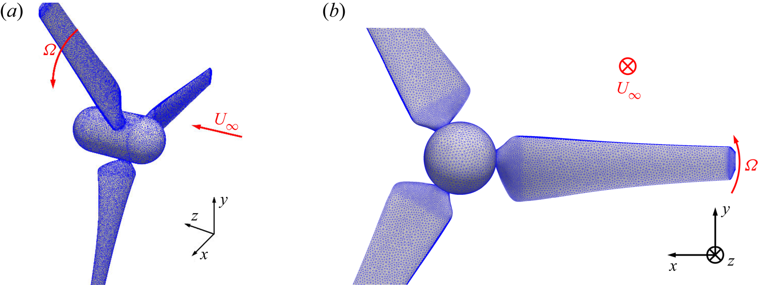
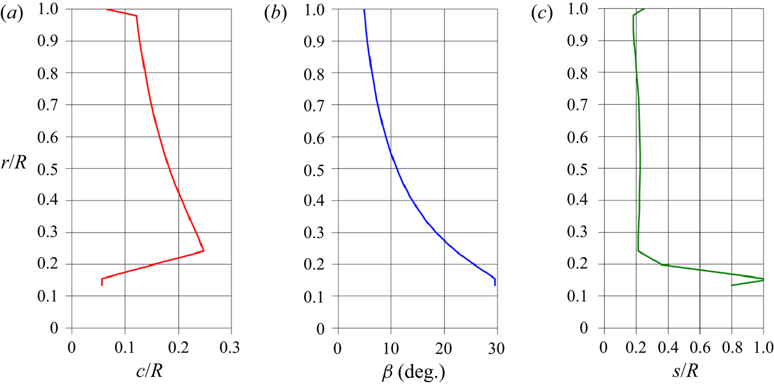
A three-bladed axial-flow hydrokinetic turbine was simulated. Figure 1 shows its geometry, represented by a surface grid composed of approximately 75 000 triangles. Note that the latter are smaller in areas of large curvature such as the tip and root of the blades. The same turbine was studied in the framework of a Round Robin experimental campaign at four facilities, as reported by Gaurier et al. (Reference Gaurier, Germain, Facq, Johnstone, Grant, Day, Nixon, Di Felice and Costanzo2015), where the parameters of global performance at several values of free-stream velocity and rotational speed of the turbine can be found. The choice of this geometry was tied to the availability of measurements from different facilities, which is not obvious, considering the relatively recent interest towards hydrokinetic turbines. As pointed out by Gaurier et al. (Reference Gaurier, Germain, Facq, Johnstone, Grant, Day, Nixon, Di Felice and Costanzo2015), actually their Round Robin campaign allowed an analysis of the sensitivity of the measurements to the particular facility where they were conducted, considering four different tanks. Compared with the classical, simplified rotor models (see Okulov, Sørensen & Wood Reference Okulov, Sørensen and Wood2015 for a review) the turbine geometry considered here features a more complex spanwise distribution of the circulation across the blades, whose maximum is located at  $70\,\%$ of the rotor radius, in contrast, for instance, with the uniform circulation assumed in the Joukowsky rotor or the Betz distribution. The cross-section of the blades was designed based on a NACA 63-418 series profile. The distributions of their chord,
 $c$, pitch angle,
 $\beta$, and thickness,
 $s$, are decreasing functions of the radial coordinate,
 $r$, as reported in detail in figure 2. It should be noted that, compared with the turbine model considered by Gaurier et al. (Reference Gaurier, Germain, Facq, Johnstone, Grant, Day, Nixon, Di Felice and Costanzo2015), the present computations considered a simplified hub geometry. In addition, the supporting stanchion in the experimental set-up was not included in the computational model.
Geometry of the turbine, including also the Lagrangian grid discretizing its surface.

Radial evolution across the span of the blades of their chord  $c$ (a), pitch angle
 $\beta$ (b) and thickness
 $s$ (c). Here,
 $R$ is the rotor radius. Data reported from Gaurier et al. (Reference Gaurier, Germain, Facq, Johnstone, Grant, Day, Nixon, Di Felice and Costanzo2015).

We considered the following values of tip speed ratio,  $TSR$, and Reynolds number,
 $Re$, for which measurements are available from Gaurier et al. (Reference Gaurier, Germain, Facq, Johnstone, Grant, Day, Nixon, Di Felice and Costanzo2015):
 \begin{equation} TSR = \frac{{\varOmega}R }{U_\infty} = 5.0 \quad Re= \frac{D U_\infty }{\nu} = 5.6 \times 10^{5}, \end{equation}
where  ${\varOmega }$ is the rotational speed of the turbine,
 $R$ its radius and
 $D$ its diameter, while
 $U_\infty$ is the free-stream velocity.
The four facilities where the measurements reported by Gaurier et al. (Reference Gaurier, Germain, Facq, Johnstone, Grant, Day, Nixon, Di Felice and Costanzo2015) were conducted are: (i) the flume tank at the French Research Institute for Exploitation of the Sea, Boulogne-Sur-Mer, France (IFREMER-FT), (ii) the flume tank at the Marine Technology Research Institute, Roma, Italy (INSEAN-FT), (iii) the towing tank at the Marine Technology Research Institute, Roma, Italy (INSEAN-TT) and (iv) the towing tank at the Kelvin Hydrodynamics Laboratory of the University of Strathclyde, Glasgow, United Kingdom (KHL-TT). In the following, comparisons with those measurements will be provided.
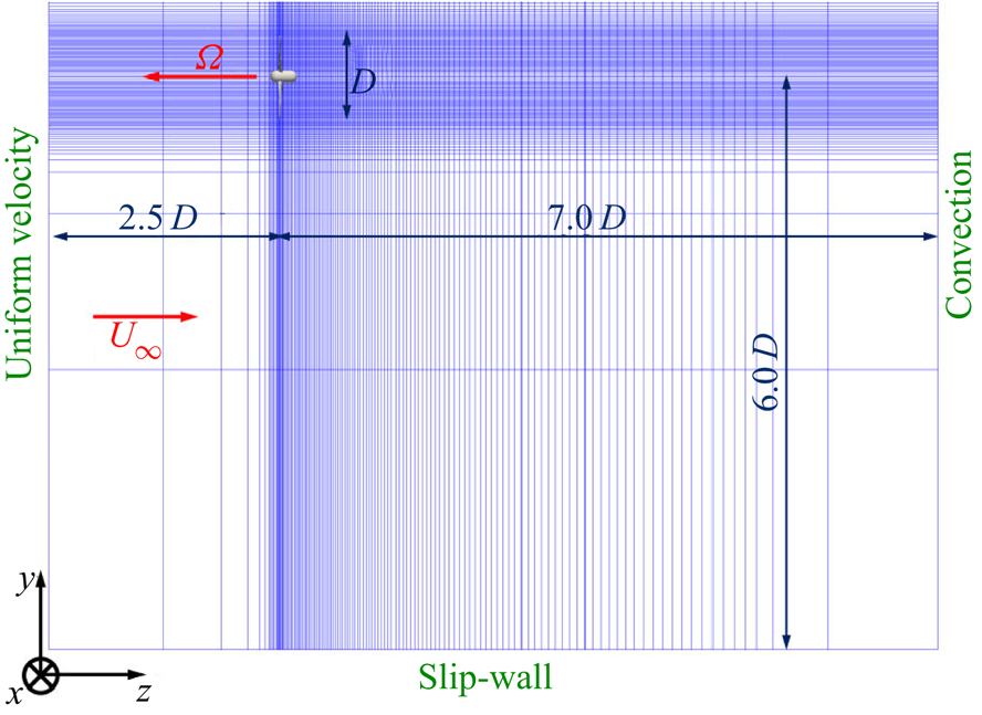
All computations were conducted on a cylindrical grid composed of approximately 1.9 billion points:  $1024\times 900\times 2048$ points across the azimuthal, radial and axial directions, respectively, resulting in a resolution over the surface of the turbine equivalent to 10 wall units. The computational domain extends from
 $2.5D$ upstream of the rotor disk up to
 $7.0D$ downstream and its radial boundary was placed at
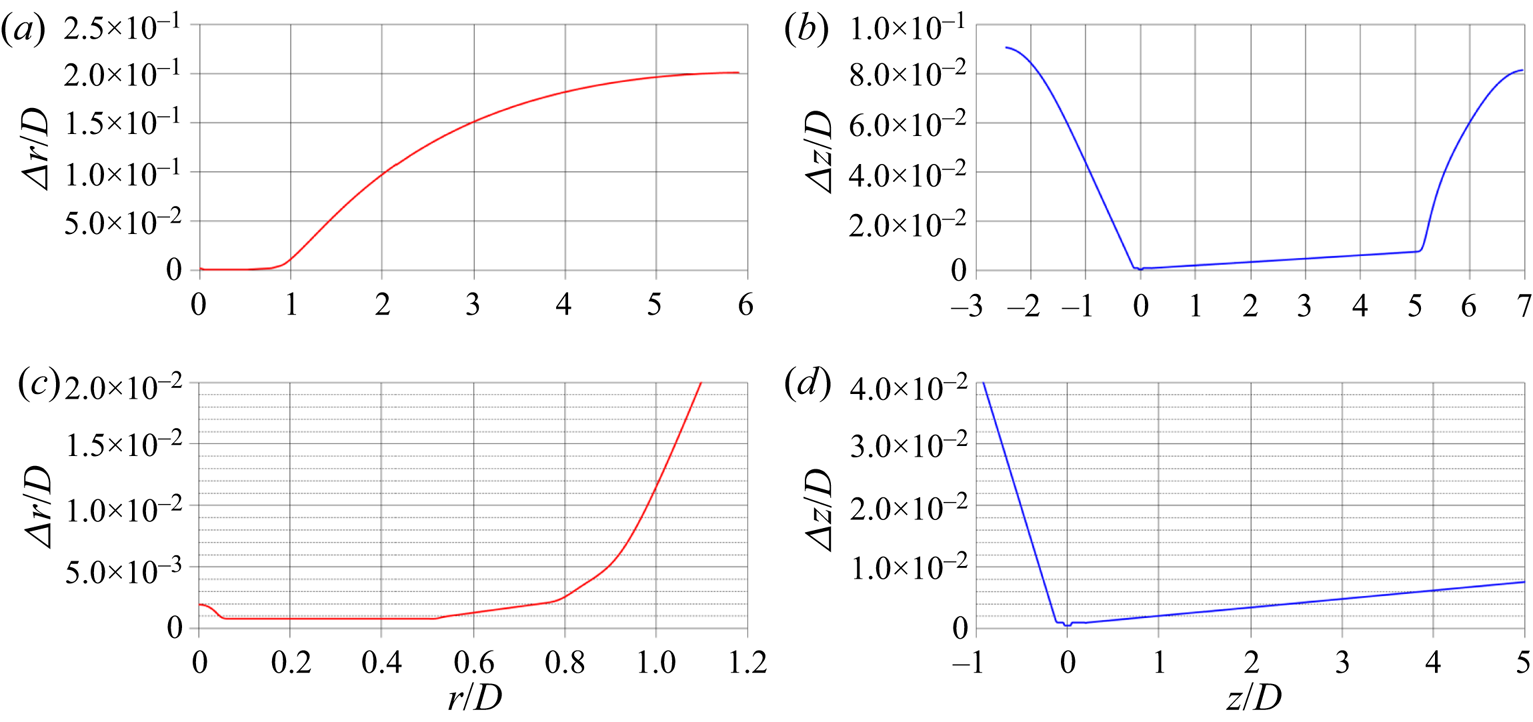
 $6.0D$ from the axis of the turbine. For the three velocity components a uniform axial velocity condition was enforced over the inlet section, slip-wall conditions with impermeability at the cylindrical boundary and convective conditions (Orlanski Reference Orlanski1976) at the outlet section. Neumann conditions were utilized for pressure and eddy viscosity across all boundaries of the domain. The grid points were uniformly spaced across the azimuthal direction, while grid stretching was exploited across both radial and axial directions, in order to cluster more points in the vicinity of the turbine. It should be also noted that, thanks to the cylindrical topology of the Eulerian grid, the uniform angular spacing across the azimuthal direction allowed grid refinement in the vicinity of the surface of the turbine, since the linear azimuthal spacing is actually decreasing from outer towards inner radii. A meridian slice of the computational grid is reported in figure 3, where only a sample of all grid points is shown, for clarity (1 out of every 16 points across both radial and axial directions). In addition, figure 4 provides the radial and axial distributions of the grid spacing, showing more details on grid stretching away from the turbine, which was placed at the origin of the reference frame. The later discussion of the results will demonstrate the suitability of the adopted grid in capturing turbulence, the tip vortices and their instability process, which are the main focus of the present study.
Meridian slice of the adopted cylindrical grid. For clarity, only 1 of every 256 points shown.

Distributions of the radial (a,c) and axial (b,d) steps of the cylindrical Eulerian grid. (a,b) whole computational domain. (c,d) details in the region including the turbine and its wake flow.

The resolution in time was also very fine, since it was tied to that in space via the Courant–Friedrichs–Lewy ( $CFL$) condition. Having adopted the RK3 scheme for the explicit discretization of all terms of radial and axial derivatives within the momentum equation, a
 $CFL=1$ requirement was enforced during the simulation. This resulted in a resolution in time requiring approximately
 $5000$ time steps of integration in time per rotation of the turbine. Computations were initially carried out for two flow-through times, to remove the memory of the initial transient. Then, after development of the wake flow, both ensemble- and phase-averaged statistics were computed on the fly during ten additional revolutions of the turbine. The computations were conducted on
 $2048$ cores of the Joliot–Curie KNL cluster, GENCI, France. Approximately twelve million core hours were utilized to generate the dataset analysed in the present study. A rough estimate of the CPU cost of a direct numerical simulation suggested that resolving the Navier–Stokes equations without filtering the smallest scales would result in a computational effort approximately 9 orders of magnitude higher. Obviously, SGS modelling is mandatory now and in the foreseeable future to make the simulation of this class of flows affordable.
4. Results
4.1. Definition of averaging operators
Statistics from the instantaneous realizations of the flow were evaluated as ensemble averages and phase averages. In the former case they were computed on the stationary Eulerian grid adopted to resolve the filtered Navier–Stokes equations, while in the latter case they were evaluated on a cylindrical grid rotating with the blades of the turbine, exploiting the symmetry of its geometry, resulting also in the statistical axisymmetry of the wake flow.
The ensemble average of any physical quantity,  $\mathscr {Q}$, was computed as
 \begin{equation} \bar{\mathscr{Q}} \left ( r, \vartheta, z \right ) = \frac{1 }{\bar{\mathscr{M}}} \sum^{\bar{\mathscr{M}}}_{i=1} \mathscr{Q} \left ( r, \vartheta, z, t_i \right ), \end{equation}
where the ensemble-averaging operator is indicated as  $\bar {\cdot }$,
 $r, \vartheta , z$ are the radial, azimuthal and axial coordinates of the cylindrical reference frame, respectively,
 $\bar {\mathscr {M}}$ is the size of the statistical sample and
 $t_i$ is the time instant of the
 $i$th solution within the sample.
Ensemble-averaged fluctuations were calculated as root-mean-squares across all instantaneous solutions
 \begin{equation} \overline{\mathscr{Q}'} \left ( r, \vartheta, z \right ) = \sqrt{ \frac{1 }{\bar{\mathscr{M}}} \sum^{\bar{\mathscr{M}}}_{i=1} \left [ \mathscr{Q} \left ( r, \vartheta, z, t_i \right ) \right ]^{2} - \left [ \bar{\mathscr{Q}} \left ( r, \vartheta, z \right ) \right ]^{2} }, \end{equation}
where the ensemble-averaged fluctuation is indicated as  $\overline {\cdot '}$.
Phase averaging was conducted as
 \begin{equation} \hat{\mathscr{Q}} ( r, \vartheta, z) = \frac{1 }{\hat{\mathscr{M}}} \sum_{i=1}^{\hat{\mathscr{M}}} \mathscr{Q} \left ( r, \vartheta + {\varOmega} t_i, z, t_i \right ), \end{equation}
where the phase-averaging operator is indicated as  $\hat {\cdot }$ and
 $\hat {\mathscr {M}}$ is the size of the statistical sample. Thanks to the symmetry of the flow problem, in the present study
 $\hat {\mathscr {M}}=\bar {\mathscr {M}}$.
Also the phase-averaged fluctuations were defined as root-mean-squares across all elements of the statistical sample
 \begin{equation} \widehat{\mathscr{Q}'} ( r, \vartheta, z) = \sqrt{ \frac{1 }{\hat{\mathscr{M}}} \sum_{i=1}^{\hat{\mathscr{M}}} \left [ \mathscr{Q} \left ( r, \vartheta + {\varOmega} t_i, z, t_i \right ) \right ]^{2} - \left [ \hat{\mathscr{Q}} \left ( r, \vartheta, z \right ) \right ]^{2} }, \end{equation}
where the phase-averaged fluctuation is indicated as  $\widehat {\cdot '}$.
Quantities that will be utilized in the following analysis of the dataset generated by LES computations include the instantaneous pressure coefficient and the phase-averaged turbulent kinetic energy. The pressure coefficient was defined as
 \begin{equation} c_p \left ( r, \vartheta, z, t \right) = \frac{p \left ( r, \vartheta, z, t \right ) - p_\infty }{0.5 \rho U_\infty^{2}}, \end{equation}
where  $p_\infty$ is the free-stream pressure, taken as the pressure at the inlet section of the computational domain, and
 $\rho$ is the fluid density.
The phase-averaged turbulent kinetic energy was computed as
 \begin{equation} \hat{k} \left ( r, \vartheta, z \right ) = \tfrac{1 }{2} \left \{ \left [ \widehat{u'} \left ( r, \vartheta, z \right ) \right ]^{2} + \left [ \widehat{v'} \left ( r, \vartheta, z \right ) \right ]^{2} + \left [ \widehat{w'} \left ( r, \vartheta, z \right ) \right ]^{2} \right \}, \end{equation}
where  $\widehat {u'}$,
 $\widehat {v'}$ and
 $\widehat {w'}$ are the phase-averaged fluctuations of the radial, azimuthal and axial velocity components in the cylindrical reference frame.
4.2. Validation with experimental results
Comparisons are presented against the experiments reported by Gaurier et al. (Reference Gaurier, Germain, Facq, Johnstone, Grant, Day, Nixon, Di Felice and Costanzo2015). They performed measurements on thrust and torque at several values of  $TSR$, including the one considered in the present study. As discussed above in § 3, they were conducted at four different facilities in the framework of a Round Robin experimental campaign, two towing tanks and two flume tanks, with the turbine immersed within a uniform flow (no mean shear), as in the present LES computations. The towing tanks measurements were not affected by free-stream turbulence. Therefore, for consistency, the measurements in the flume tanks were carried out with the lowest possible turbulence levels, corresponding to values of turbulent kinetic energy equal to
 $0.09\,\%$ and
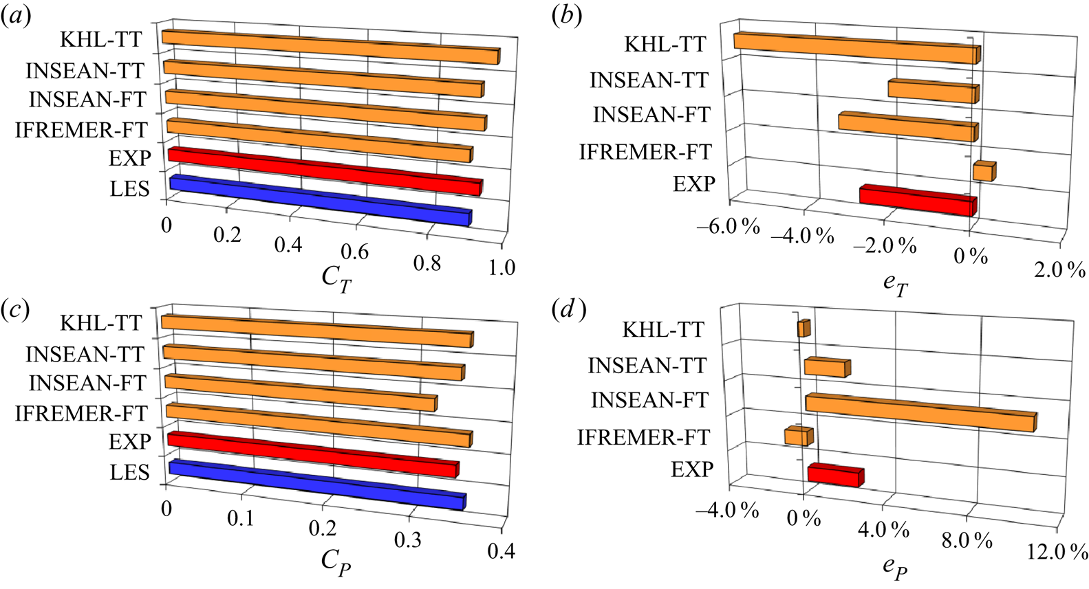
 $0.14\,\%$ at INSEAN and IFREMER, respectively. During the experiments the rotor was connected to a direct-current motor and a control unit was utilized to enforce its rotational speed. In a similar way, in the present computations the rotational speed of the Lagrangian grid representing the rotor was prescribed. Figure 5 reports comparisons between the LES results and the four experiments for both thrust and power coefficients in (a,b) and (c,d), respectively. The thrust and power coefficients were defined as
 \begin{equation} C_T=\frac{T }{0.5 \rho A U_\infty^{2}}, \quad C_P = \frac{M {\varOmega} }{0.5 \rho A U_\infty^{3}}, \end{equation}
where  $T$ and
 $M$ are the dimensional thrust and torque on the turbine and
 $A$ is its frontal area. It should be noted that the hub geometries of the turbine model studied by Gaurier et al. (Reference Gaurier, Germain, Facq, Johnstone, Grant, Day, Nixon, Di Felice and Costanzo2015) and the one considered in the present computational set-up were different. In addition, the LES computations did not include the supporting stanchion. Therefore, the data from Gaurier et al. (Reference Gaurier, Germain, Facq, Johnstone, Grant, Day, Nixon, Di Felice and Costanzo2015) were properly adjusted, for comparison purposes with our computational results. This was not necessary for the reported torque, since the axial moments produced by the hub and the stanchion are negligible. However, since they generate a significant amount of drag, a correction was required on the thrust. Its value on the support and the hub, in the absence of the blades of the turbine, was measured at IFREMER. It was removed from all experimental values of thrust. For the numerical results only the value of the axial force acting on the blades of the turbine was taken into account. This way, the comparison of the thrust coefficients between experiments and computations can be considered consistent.
(a,c) Ensemble-averaged values of thrust (a) and power (c) coefficients. (b,d) Percentage error of the LES results, relative to the experiments. LES: present results; EXP: average across the four experimental facilities; IFREMER-FT: measurement at the IFREMER flume tank; INSEAN-FT: measurement at the INSEAN flume tank; INSEAN-TT: measurement at the INSEAN towing tank; KHL-TT: measurement at the KHL towing tank.

Figure 5(a,c) shows the ensemble-averaged values of thrust and power coefficients. In each panel the column labelled as EXP reports the average across the four facilities where measurements were conducted. Figure 5(b,d) reports the percentage errors of the LES results, relative to the experiments. They were computed as
 \begin{equation} e_T=\frac{C_T^{LES} - C_T^{EXP} }{C_T^{EXP}} \times 100, \quad e_P=\frac{C_P^{LES} - C_P^{EXP} }{C_P^{EXP}} \times 100, \end{equation}
where the superscripts  $LES$ and
 $EXP$ stand for the numerical and experimental values, respectively. The thrust coefficient from the LES computation,
 $\bar {C}_T=0.9060$, is within the range of the experimental values,
 $0.9022 < \bar {C}_T < 0.9618$. The average experimental value is
 $\bar {C}_T=0.9311$, with a relative error
 $e_T = -2.69\,\%$. Also the power coefficient from the simulations,
 $\bar {C}_P=0.3564$, is bounded by the minimum and maximum values from the experiments, in the range
 $0.3219 < \bar {C}_P < 0.3605$. The average across all experiments is
 $\bar {C}_P=0.3474$, resulting in a relative error
 $e_P = 2.61\,\%$. It is also worth noting that the average error for
 $\bar {C}_T$ is biased towards larger values by the measurements from the KHL towing tank, reporting a value for the thrust coefficient significantly higher, compared with all other experiments and computations. This is even more evident for the power coefficient. The average from the experiments is indeed shifted towards smaller values by the
 $\bar {C}_P$ reported from the measurements conducted at the INSEAN flume tank. Thus, the overall agreement of the LES results with the experiments in terms of parameters of global performance is good, especially taking into account that the LES values of thrust and power coefficients fall within the range across the experiments reported by Gaurier et al. (Reference Gaurier, Germain, Facq, Johnstone, Grant, Day, Nixon, Di Felice and Costanzo2015).
4.3. Instability of the tip vortices
4.3.1. Instantaneous visualizations
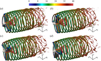
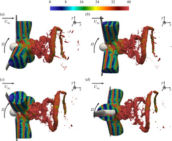
Instantaneous visualizations of the tip vortices are provided in figure 6, where isosurfaces of pressure were coloured using the vorticity magnitude. It is clear that, just downstream of the rotor disk, the tip vortices are very coherent and their helical trajectory very stable. It should be also noted that, in this particular case, the hub vortex is not as strong and coherent, although this likely depends on the particular hub geometry. Thus, the wake flow is dominated by the dynamics of the tip vortices. Moving downstream, their trajectory starts developing instabilities, as shown by deviations from the helix originating from the tip of the blades. This promotes mutual inductance between tip vortices, since they come closer to each other, which amplifies the instability of the wake system. This observation is in agreement with the work by Widnall (Reference Widnall1972), where the short- and long-wave instabilities of the tip vortices (indicated as  $\boldsymbol {SWI}$ and
 $\boldsymbol {LWI}$ hereafter) are identified as the original source of interaction between them, leading to mutual inductance phenomena (
 $\boldsymbol {MI}$). Quickly, leapfrogging and vortex meandering develop, leading to breakdown into smaller structures, loss of coherence and initiating the process of wake contraction and momentum recovery. These phenomena are very similar to those observed experimentally in the time-resolved visualizations of propeller wakes by Felli et al. (Reference Felli, Camussi and Di Felice2011). Earlier LES computations by Ivanell et al. (Reference Ivanell, Mikkelsen, Sørensen and Henningson2010), Sarmast et al. (Reference Sarmast, Dadfar, Mikkelsen, Schlatter, Ivanell, Sørensen and Henningson2014) and Sørensen et al. (Reference Sørensen, Mikkelsen, Henningson, Ivanell, Sarmast and Andersen2015), coupled with an actuator line technique to represent the blades of a wind turbine, have also reported a similar behaviour. However, in those simulations, perturbations were introduced to trigger the instability of the tip vortices, which would otherwise remain stable across the whole extent of the computational domain. In addition, those computations were able to reproduce the leapfrogging mechanism and eventual breakdown of the tip vortices across shorter distances downstream of destabilization, likely due to limitations in terms of grid resolution.
Instantaneous isosurfaces of pressure ( $c_p=-0.4$), coloured by vorticity magnitude. Vorticity scaled by
 $U_\infty /D$. Phase angle of the rotor indicated by
 $\varphi$.
 $(a)\ \varphi = 0^{\circ},\, (b)\ \varphi = 90^{\circ},\, (c)\ \varphi = 180^{\circ}, (d)\ \varphi = 270^{\circ}$.

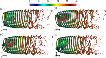
Due to the complexity of the wake system, especially downstream of the development of instability, figure 7 provides an alternative view angle of the tip vortices in figure 6. Figure 7 is especially useful to highlight the leapfrogging mechanism, with the tip vortices exchanging their relative position across the streamwise direction. The minor role of the hub vortex in the present case is again clear. This result is an indirect confirmation of the findings by Felli et al. (Reference Felli, Camussi and Di Felice2011), who reported that the instability of the system of tip vortices seemed to occur before that of the hub vortex (in that case stronger than in the present results), suggesting that the mutual inductance between them was the driving source of destabilization, rather than their interaction with the hub vortex. Instability was indeed observed to occur earlier for shorter inter-spiral distances, achieved at higher load conditions or with geometries consisting of more blades (Felli et al. Reference Felli, Guj and Camussi2008, Reference Felli, Camussi and Di Felice2011). In addition, the visualizations in figure 7 are consistent with the conclusions from the recent theoretical and experimental study by Quaranta et al. (Reference Quaranta, Brynjell-Rahkola, Leweke and Henningson2019). They reported that local pairing is a mechanism leading to a strong amplification of the deformations of the helices of the tip vortices and eventually their break-up. This is also observed in figure 7: once local pairing of tip vortices has occurred, the process of destabilization of the overall system develops very quickly, producing large, intricate deviations from the original helical trajectory and starting the process of break-up of the tip vortices into smaller structures.
Instantaneous isosurfaces of pressure ( $c_p=-0.4$), coloured by vorticity magnitude. Vorticity scaled by
 $U_\infty /D$. Phase angle of the rotor indicated by
 $\varphi$. Same data as figure 6 in lateral view.
 $(a)\ \varphi = 0^{\circ}, (b)\ \varphi = 90^{\circ},\, (c)\ \varphi = 180^{\circ},\, (d)\ \varphi = 270^{\circ}$.

For a better understanding, details of the panels in figure 7 are reported in figure 8, where actually a higher value (in magnitude) of the pressure coefficient was considered for the isosurfaces, in order to better isolate the core of the tip vortices. Figure 8 shows that the instability of the tip vortices usually starts as short-wave instabilities, having a wavelength of a few core diameters. Then, long-wave instabilities develop, as deviations from the initial helical trajectory, featuring wavelengths of several core diameters. When this occurs the density of the short-wave instabilities across each tip vortex is also increased, suggesting a mechanism of mutual amplification of these two modes of instability. Then, the long-wave instabilities eventually lead to mutual inductance between tip vortices, having the evident effect of further amplifying the long-wave instabilities, causing vortex meandering. This result is in fairly good agreement with the experiments conducted by Quaranta, Bolnot & Leweke (Reference Quaranta, Bolnot and Leweke2015) on the helical vortex generated by a single-bladed rotor, where small perturbations were introduced and their effect on the streamwise evolution of the tip vortex observed. Quaranta et al. (Reference Quaranta, Bolnot and Leweke2015) have shown that the sensitivity to long-wave instabilities is very strong and also small perturbations are able to produce a totally different evolution, compared with the baseline unperturbed one, resulting in coupling and leapfrogging between neighbouring loops of the same vortex.
Detail of figure 7: instantaneous isosurfaces of pressure ( $c_p=-0.8$), coloured by vorticity magnitude. Vorticity scaled by
 $U_\infty /D$. Phase angle of the rotor indicated by
 $\varphi$. Here,
 $\boldsymbol {LWI}$,
 $\boldsymbol {MI}$ and
 $\boldsymbol {SWI}$ are long-wave instabilities, mutual inductance and short-wave instabilities, respectively.
 $(a)\ \varphi = 0^{\circ}, (b)\ \varphi = 90^{\circ},\, (c)\ \varphi = 180^{\circ},\, (d)\ \varphi = 270^{\circ}$.

In figure 9 a lower value (in magnitude) of the pressure coefficient was selected to extract the tip vortices. Although this choice leads to a higher level of saturation, preventing us from isolating the core of the coherent structures, it allows following their evolution further downstream. This way, figure 9 reveals that wider areas of low pressure develop as the process of instability is initiated. They come from mutual interaction and coupling between tip vortices, which is a phenomenon observed in experiments dealing with both axial-flow turbines (Hong et al. Reference Hong, Toloui, Chamorro, Guala, Howard, Riley, Tucker and Sotiropoulos2014; Lignarolo et al. Reference Lignarolo, Ragni, Scarano, Simão Ferreira and Van Bussel2015; Lust et al. Reference Lust, Flack and Luznik2018, Reference Lust, Flack and Luznik2020) and marine propellers (Felli et al. Reference Felli, Camussi and Di Felice2011). These large structures eventually break down into smaller eddies, resulting in a diffused region of large vorticity and turbulent stresses at the outer radii, as discussed more in detail in the next sections. The instability of the system of tip vortices, observed in figure 9, is coupled with the beginning of the process of momentum recovery and wake contraction, as demonstrated by the migration of the smaller structures originating from the breakdown of the tip vortices towards inner radial coordinates.
Instantaneous isosurfaces of pressure ( $c_p=-0.2$), coloured by vorticity magnitude. Vorticity scaled by
 $U_\infty /D$. Phase angle of the rotor indicated by
 $\varphi$. Same data as figure 6 in lateral view.
 $(a)\ \varphi = 0^{\circ}, (b)\ \varphi = 90^{\circ},\, (c)\ \varphi = 180^{\circ},\, (d)\ \varphi = 270^{\circ}$.

It is worth noting that the many instantaneous realizations of the flow from the solution of the filtered Navier–Stokes equations allowed us to visualize in detail the streamwise evolution of the structures populating the wake. They pointed to the lack of wake meandering, which is a quite typical behaviour for axial-flow turbines. This may be the consequence of both the uniformity of the flow where the present rotor operates and the symmetry of the considered geometry, not having included in the turbine model the influence of the support. It is likely that such conditions introduce a delay in the development of wake meandering, requiring a larger downstream distance to develop than that available within the adopted computational domain. This hypothesis is supported by the results reported in the literature. For instance, the experimental study by Chamorro et al. (Reference Chamorro, Hill, Morton, Ellis, Arndt and Sotiropoulos2013) discussed the existence of two different regions of the wake of an axial-flow hydrokinetic turbine: the near wake, up to three diameters downstream, and the far wake. The former was characterized by the tip vortices, the latter by wake meandering, downstream of the instability of the tip vortices. This meandering consisted of lateral oscillations of the wake, characterized by small frequencies, corresponding to a value of the Strouhal number equal to 0.28, based on the inflow velocity at the hub height and the diameter of the turbine, close to that observed in the wake of bluff bodies. Similar results were also reported by Kang et al. (Reference Kang, Yang and Sotiropoulos2014) via LES computations. In addition, they revealed the importance of the hub vortex in promoting the wake instability and its transition to meandering behaviour. They also found that the use of simplified actuator line or actuator disk models, rather than geometry-resolving approaches, delays and underestimates wake meandering, which Kang et al. (Reference Kang, Yang and Sotiropoulos2014) found especially dependent on the interaction of the hub vortex with the tip vortices and the specific geometrical details of the turbine. The importance of the hub vortex in the onset of wake meandering was also verified downstream of a wind turbine in the experimental study by Howard et al. (Reference Howard, Singh, Sotiropoulos and Guala2015), who also reported that this behaviour is strongly dependent on the particular case. Kang et al. (Reference Kang, Yang and Sotiropoulos2014) acknowledged indeed that the location of wake transition and the amplitude of meandering motions are specific features of each turbine and its geometry. This was also observed for cross-flow turbines (Araya, Colonius & Dabiri Reference Araya, Colonius and Dabiri2017; Posa Reference Posa2020a), where the near wake, featuring well distinguishable columnar vortices originating from the stall of the blades, switches to a far wake, resembling that of a bluff body and affected by meandering motions. Also in those studies it was found that the streamwise location of this transition is case dependent and is affected by several parameters, such as the turbine geometry and its rotational speed. However, for cross-flow turbines the onset of wake meandering is accelerated by the inherent asymmetry of the wake between its leeward and windward sides.
In the present case, not having included asymmetries in both inflow conditions and turbine geometry has likely the effect of delaying the development of meandering motions. For instance, extensive experiments by Heisel, Hong & Guala (Reference Heisel, Hong and Guala2018) on wind turbines pointed out the importance of the operating conditions, including not only the level of load on the rotor blades, but also the ingested large-scale turbulence, in triggering wake meandering phenomena. The inflow turbulence contributes to start oscillations of the wake by promoting the instability of the annular shear layer at its boundary. In addition, Kang et al. (Reference Kang, Yang and Sotiropoulos2014) and Howard et al. (Reference Howard, Singh, Sotiropoulos and Guala2015) found the hub vortex, interacting with the tip vortices, especially important in triggering transition and wake meandering downstream of both hydrokinetic and wind turbines. In contrast, for the rotor we simulated, the hub vortex played a rather minor role in the overall wake dynamics. However, it should be recalled that our study is focused on the physics of the near wake and in particular on the instability of its tip vortices, in a region where also the earlier works by Chamorro et al. (Reference Chamorro, Hill, Morton, Ellis, Arndt and Sotiropoulos2013) and Kang et al. (Reference Kang, Yang and Sotiropoulos2014) on hydrokinetic turbines, those by Howard et al. (Reference Howard, Singh, Sotiropoulos and Guala2015) and Heisel et al. (Reference Heisel, Hong and Guala2018) on wind turbines, as well as that by Felli et al. (Reference Felli, Camussi and Di Felice2011) on marine propellers, have observed no wake meandering behaviours.
4.3.2. Streamwise evolution of the tip vortices
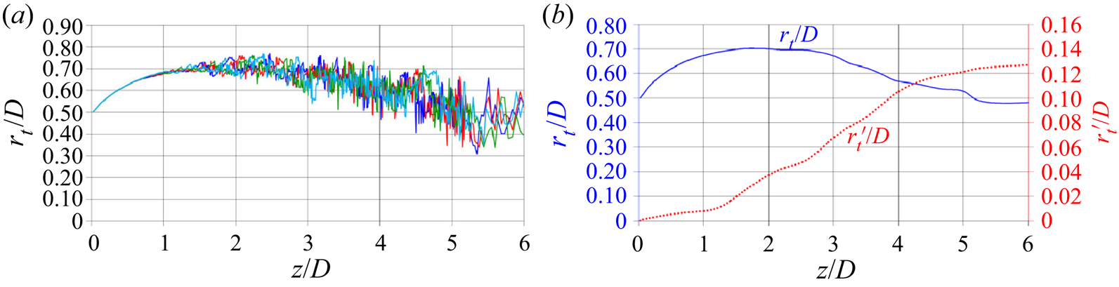
A more quantitative representation of the growing instability of the tip vortices away from the rotor disk is provided in figure 10. In (a) the radial location of the core of the tip vortices, as a function of the streamwise coordinate downstream of the turbine, is shown for the four instantaneous realizations of the flow considered in figures 6–9. The tip vortices were identified considering the radial position of the minima within the pressure field for each streamwise coordinate. For each case they were averaged across the three tip vortices shed by the blades of the turbine. In the region  $0 < z/D < 1$ the wake experiences an expansion, as a consequence of the deceleration of the flow produced by the turbine. The trajectory of the tip vortices is very stable and the instantaneous results practically overlap each other. Starting at
 $z/D \approx 1$ the oscillations of the trajectories of the tip vortices become more evident, gradually growing in amplitude. It is clear that the instantaneous solutions do not overlap anymore. Interestingly, for
 $z/D>2.5$, the process of instability of the system of tip vortices is coupled with a contraction of the outer boundary of the wake and influx of higher-momentum fluid from the free stream, feeding the process of wake recovery.
(a) Streamwise evolution of the radial locations of the core of the tip vortices from the instantaneous realizations of the flow in figures 6–9. For each case we show the average across the three tip vortices shed by the blades of the turbine. (b) Streamwise evolution of the phase-averaged radial location of the core of the tip vortices ( $r_t/D$, left vertical axis) and its root-mean-square (
 $r_t'/D$, right vertical axis).

In figure 10(b) the phase-averaged values of the radial coordinates of the core of the tip vortices and their root-mean-squares, computed across 720 instantaneous realizations of the flow through 10 revolutions of the turbine, are reported. They confirm the wake expansion up to  $z/D \approx 1.5$, the presence of a region of plateau of the mean radial location between
 $1.5 < z/D < 2.5$ and eventually the contraction further downstream. This behaviour is consistent with that hypothesized by Medici (Reference Medici2005) and observed in the experiments on the wake of an axial-flow wind turbine by Lignarolo et al. (Reference Lignarolo, Ragni, Scarano, Simão Ferreira and Van Bussel2015). They pointed to the role of the tip vortices across the region just downstream of the turbine, where they act as a ‘shield’ between the higher-momentum fluid populating the free stream and the lower-momentum fluid within the core of the wake, delaying the process of momentum recovery. In contrast, when the process of instability fully develops, the intense mixing within the shear layer at the outer boundary of the wake promotes wake contraction, due to both convective and turbulent transport from the outer radii towards the inner ones.
The streamwise evolution of the root-mean-squares of the radial coordinate of the core of the tip vortices provides also interesting information. The process of destabilization of the tip vortices is actually gradual, as demonstrated by the positive slope of the fluctuations across the whole streamwise extent of the wake. This was also shown for the case of an axial-flow wind turbine by Sherry et al. (Reference Sherry, Nemes, Lo Jacono, Blackburn and Sheridan2013) via PIV measurements. However, it is clear that at  $z/D \approx 1.5$ such a process undergoes an evident acceleration. The results discussed above suggest that the faster growth of the fluctuations affecting the trajectory of the tip vortices starts when the deviations from the mean helix become large enough to allow mutual inductance between tip vortices, substantially amplifying the process of their destabilization and increasing vortex meandering.
4.3.3. Power spectral densities
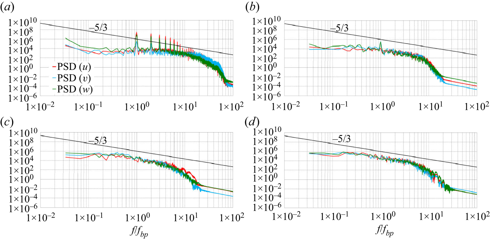
The power spectral densities of the radial, azimuthal and axial velocity components are shown in figure 11 at four locations within the wake of the turbine of radial coordinate  $r/D=0.6$ and axial coordinates
 $z/D=0.4$ (figure 11a),
 $z/D=1.0$ (figure 11b),
 $z/D=2.0$ (figure 11c) and
 $z/D=3.0$ (figure 11d). In each panel of figure 11 the
 $-5/3$ slope of the inertial range of frequencies from the Kolmogorov theory on homogeneous, isotropic turbulence is also reported. The horizontal axes were scaled based on the frequency of the passage of the blades of the turbine,
 $f_{bp}$. In figure 11(a), the spectra are obviously dominated by the tip vortices. Evident peaks occur for all velocity components at the frequency of the blade passage and at several higher harmonics. It should be noted that the power spectral densities in figure 11(a) do not reproduce the
 $-5/3$ slope, since turbulence at this streamwise location within the wake is still very far from isotropy, due to the strong coherence of the flow, as also demonstrated in the next section. The behaviour observed in figure 11(b) is already substantially different. Peaks are still distinguishable at the frequency of the blade passage, but they are definitely weaker than at the upstream location considered in figure 11(a). No maxima at higher harmonics are visible anymore, confirming that the wake flow already experienced a significant reduction of its coherence. Instead, the inertial range of frequencies in figure 11(b) shows a behaviour much more consistent with the
 $-5/3$ slope, demonstrating that: (i) the process of instability of the tip vortices produces smaller scales, leading to more homogeneous and isotropic turbulence at the outer radii of the wake; (ii) the adopted resolution is suitable to capture accurately the process of energy cascade typical of turbulence across a wide range of scales and frequencies. Moving further downstream, both figure 11(c) and figure 11(d), where no peaks are visible anymore, demonstrate: (i) the lack of large-scale coherence of the wake flow corresponding to the frequency of the blade passage, due to the upstream destabilization of the system of tip vortices; (ii) the presence of an evident, wide inertial range of frequencies with the expected slope.
Power spectral density (PSD) of the three velocity components within the wake of the turbine at  $r/D=0.6$ and
 $z/D=0.4$ (a),
 $z/D=1.0$ (b),
 $z/D=2.0$ (c) and
 $z/D=3.0$ (d). Also the
 $-5/3$ slope from Kolmogorov's theory on homogeneous, isotropic turbulence is reported. Horizontal axes scaled by the frequency of the blade passage,
 $f_{bp}$.

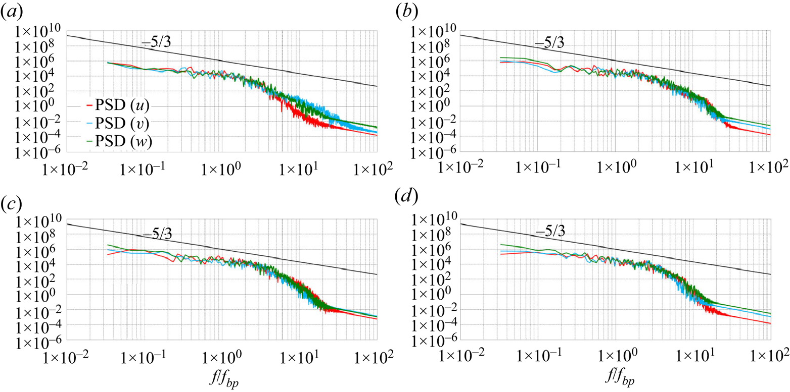
Additional evidence of the quality of the computational grid is provided in figure 12, where the PSDs for the three velocity components are reported at 5 diameters downstream of the turbine. Four radial positions are considered at  $r/D=0.0$ (figure 12a),
 $r/D=0.2$ (figure 12b),
 $r/D=0.4$ (figure 12c) and
 $r/D=0.6$ (figure 12d). These are locations away from the region of major focus of the present study, where the instability of the tip vortices develops (
 $1 < z/D < 2$), and rather close to the outflow boundary of the computational domain (
 $z/D=7$). Although there the grid resolution is relatively coarse, compared with the streamwise locations populated by the system of coherent tip vortices, the results in all panels of figure 12 demonstrate that the adopted resolution is still suitable to resolve a wide range of scales.
PSD of the three velocity components within the wake of the turbine at  $z/D=5.0$ and
 $r/D=0.0$ (a),
 $r/D=0.2$ (b),
 $r/D=0.4$ (c) and
 $r/D=0.6$ (d). Also the
 $-5/3$ slope from Kolmogorov's theory on homogeneous, isotropic turbulence is reported. Horizontal axes scaled by the frequency of the blade passage,
 $f_{bp}$.

4.3.4. Hub vortex
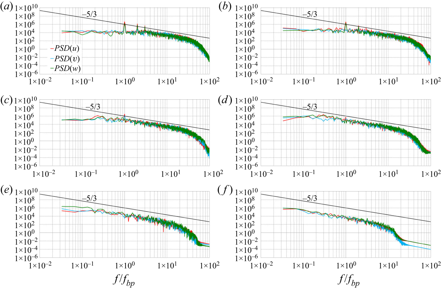
As discussed above, the hub vortex has a minor impact in the present case on the wake dynamics. PSDs in the vicinity of the wake axis are illustrated in figure 13. They are reported at the radial coordinate  $r/D=0.1$ between the streamwise coordinates
 $z/D=0.1$ and
 $z/D=1.0$. Figure 13(a) deals with
 $z/D=0.1$, which is a position placed upstream of the tail of the hub, located at
 $z/D=0.18$. PSDs are considered at this position to help distinguish the contribution by the vortices from the root of the blades from that of the hub vortex, which is obviously absent in figure 13(a). In this panel, clear peaks are visible at
 $f_{bp}$,
 $2\,f_{bp}$ and
 $3\,f_{bp}$. In figure 13(b) a location just downstream of the tail of the hub is considered, at
 $z/D=0.2$. Those peaks are weaker, especially at
 $2\,f_{bp}$ and
 $3\,f_{bp}$. An increase of the energy at
 $f< f_{bp}$ is observed, compared with the upstream location, although no evident peak is visible at smaller frequencies such as, for instance, at the frequency of the rotation of the turbine. Actually, the signature of the hub vortex at small frequencies is more evident further downstream, at
 $z/D=0.3$ in figure 13(c), where small peaks close to
 $f_{bp}/3$ can be noticed. However, this is already not the case at
 $z/D=0.4$ in figure 13(d), where turbulence already follows very closely Kolmogorov's slope of homogeneous, isotropic turbulence. This trend is reinforced further downstream at
 $z/D=0.5$ (figure 13e) and
 $z/D=1.0$ (figure 13f). Overall, it is clear that the hub vortex in the present case is not a dominant wake feature.
PSD of the three velocity components within the wake of the turbine at  $r/D=0.1$ and
 $z/D=0.1$ (a),
 $z/D=0.2$ (b),
 $z/D=0.3$ (c),
 $z/D=0.4$ (d)
 $z/D=0.5$ (e) and
 $z/D=1.0$ (f). Also the
 $-5/3$ slope from Kolmogorov's theory on homogeneous, isotropic turbulence is reported. Horizontal axes scaled by the frequency of the blade passage,
 $f_{bp}$.

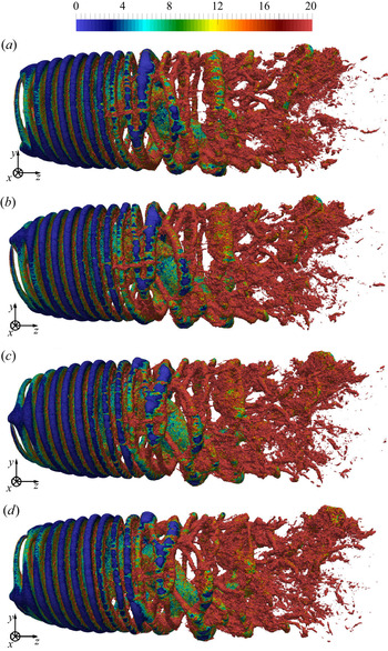
The detail of the wake core is illustrated in figure 14, again using instantaneous isosurfaces of the pressure coefficient for the same instants in time considered in the earlier visualizations. For visibility of the inner structures, the flow fields at the outer radii ( $r>0.8R$) are blanked out, to remove the tip vortices. It is clear that the same topology repeats consistently during the rotation of the turbine. Coherent structures originate from the hub, but they populate just the region immediately downstream of the rotor and are unable to affect the tip vortices and their instability. This result suggests that, although the hub vortex may in some cases, depending on the working conditions and the geometry of the turbine, promote the phenomena of instability of the system of tip vortices, as demonstrated by Kang et al. (Reference Kang, Yang and Sotiropoulos2014) for a hydrokinetic turbine, they are an inherent feature of the wake.
Instantaneous isosurfaces of pressure ( $c_p=-0.4$), coloured by vorticity magnitude. Phase angle of the rotor indicated by
 $\varphi$. Same data as figure 6: detail of the wake core. For visibility of the inner wake, the flow field at outer radii (
 $r>0.8R$) is blanked out. Vorticity scaled by
 $U_\infty /D$.
 $(a)\ \varphi = 0^{\circ},\, (b)\ \varphi = 90^{\circ}, (c)\ \varphi = 180^{\circ},\, (d)\ \varphi = 270^{\circ}$.

4.4. Correlation between instability and Reynolds stresses
A strong correlation between the instability of the tip vortices and the turbulent stresses at the outer wake boundary was found from the analysis of the statistics.
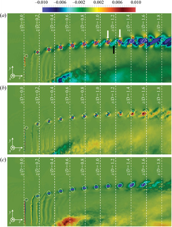
Figure 15 shows the phase-averaged contours of the turbulent shear stresses on a meridian slice, with a special focus on their evolution within the tip vortices. It should be noted that, for visualization purposes, the colour scale was saturated and more quantitative details on the actual peaks of the Reynolds stresses at the core of the tip vortices will be provided later. In figure 15, isolines of the pressure are also shown, to highlight the cores of the tip vortices, up to the development of instability phenomena. Further downstream, the synchronization with the rotation of the blades of the turbine is lost and phase averages become actually equivalent to ensemble averages. It should be also noted that the values of pressure within the wake core are higher, resulting in no isolines at inner radial locations, confirming that, in the present case, the hub vortex is weak.
Phase-averaged contours of the shear Reynolds stresses on a meridian plane through the axis of the turbine:  $\widehat {u'w'}$ (a),
 $\widehat {u'v'}$ (b) and
 $\widehat {v'w'}$ (c). Isolines for a value of the pressure coefficient
 $\hat {c}_p=-0.4$. In panel (a) the white arrows indicate two consecutive signatures of the tip vortices and the black arrow the region of shear between them. Values of turbulent stresses scaled by
 $U_\infty ^{2}$.

It is clear that the highest values of turbulence are achieved at the outer radii within the core of the tip vortices. The behaviour of  $\widehat {u'w'}$ in figure 15(a) is especially interesting. Just downstream of the turbine it displays a positive peak at the core of the tip vortices. However, a growing region of negative values of shear stress develops between them, becoming gradually higher moving away from the turbine (see for instance the black arrow between the tip vortices indicated by white arrows). It is evident that each tip vortex moves downstream faster than the shear layer from the trailing edge of each blade, coming closer to the wake shed by the preceding blade and starting a roll-up process. This way, the outer region of the wake of each blade becomes a ‘bridge’ between consecutive tip vortices, where the values of shear stress experience an increase moving downstream. Therefore, the large positive and negative values of
 $\widehat {u'w'}$ within each tip vortex and between them, respectively, come from different sources: the former are due to the process of roll-up of vorticity coming from the tip of the blades, while the latter from the increasing shear developing between the neighbouring helices of the tip vortices. It is also interesting to notice that the shear between the tip vortices becomes gradually dominant, as demonstrated by the contours in figure 15(a), switching sign within the vortex cores in the region of streamwise coordinates where we verified the full development of instability phenomena (§ 4.3). It is also important to notice that the same streamwise evolution of
 $\widehat {u'w'}$ was observed in the PIV experiments by Lignarolo et al. (Reference Lignarolo, Ragni, Krishnaswami, Chen, Simão Ferreira and van Bussel2014) for the wake of an axial-flow wind turbine. Thus, the visualization in figure 15(a) suggests that the shear between tip vortices across the radial and streamwise directions is promoted by their roll-up with the outer region of the shear layer shed by the preceding blade and is gradually triggering their instability. This was hypothesized by Di Felice et al. (Reference Di Felice, Di Florio, Felli and Romano2004) and Felli et al. (Reference Felli, Guj and Camussi2008, Reference Felli, Camussi and Di Felice2011) also for the tip vortices shed by marine propellers. They found this hypothesis consistent with the faster instability in the presence of more blades and at higher loads. Of course, in the wake of propellers, which accelerate the flow, in contrast with turbines, the interaction of the tip vortices occurs with the wake of the following blade. This was also confirmed by the LES computations on the INSEAN E1658 propeller by Posa et al. (Reference Posa, Broglia and Balaras2019a, Reference Posa, Broglia, Felli, Falchi and Balarasb), but to the authors’ knowledge has never been reported before in the case of axial-flow turbines. Nonetheless, the present results highlight further the similarity between the wakes of propellers and axial-flow turbines. It is also interesting to notice that phenomena of shear by the tip vortices with the wake of the neighbouring blades are promoted, as the wake develops downstream, not only by the difference in their pitch, but also by the growing size of the core of the tip vortices, due to diffusion phenomena. This behaviour was recently discussed by Okulov et al. (Reference Okulov, Kabardin, Mikkelsen, Naumov and Sørensen2018) and can be observed in figure 15 and in figure 16, looking at both the isolines of pressure and the maxima of shear and normal stresses identifying at outer radii the core of the tip vortices.
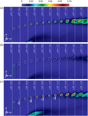
Phase-averaged contours of the normal Reynolds stresses on a meridian plane through the axis of the turbine:  $\widehat {u'u'}$ (a),
 $\widehat {v'v'}$ (b) and
 $\widehat {w'w'}$ (c). Isolines for a value of the pressure coefficient
 $\hat {c}_p=-0.4$. Values of turbulent stresses scaled by
 $U_\infty ^{2}$.

The behaviour of the shear stresses  $\widehat {u'v'}$ and
 $\widehat {v'w'}$ in figure 15(b) and figure 15(c), respectively, is actually rather different from that of
 $\widehat {u'w'}$, with negative peaks within the tip vortices, declining as their coherence is lost. Both figure 15(b) and figure 15(c) do not display the areas of large turbulent stresses in the region of shear between tip vortices, visible in figure 15(a), pointing to the special role of
 $\widehat {u'w'}$ in their process of destabilization.
The gradual development of instability by the tip vortices is also demonstrated by the normal Reynolds stresses in figure 16. It is clear that they are dominated by those of the radial (figure 16a) and streamwise (figure 16c) velocity components. In particular, the peaks observed at the core of the tip vortices spread to wider areas as they move away from the wake generator, which is a signature of the increasing oscillations of their trajectory around the mean helix.
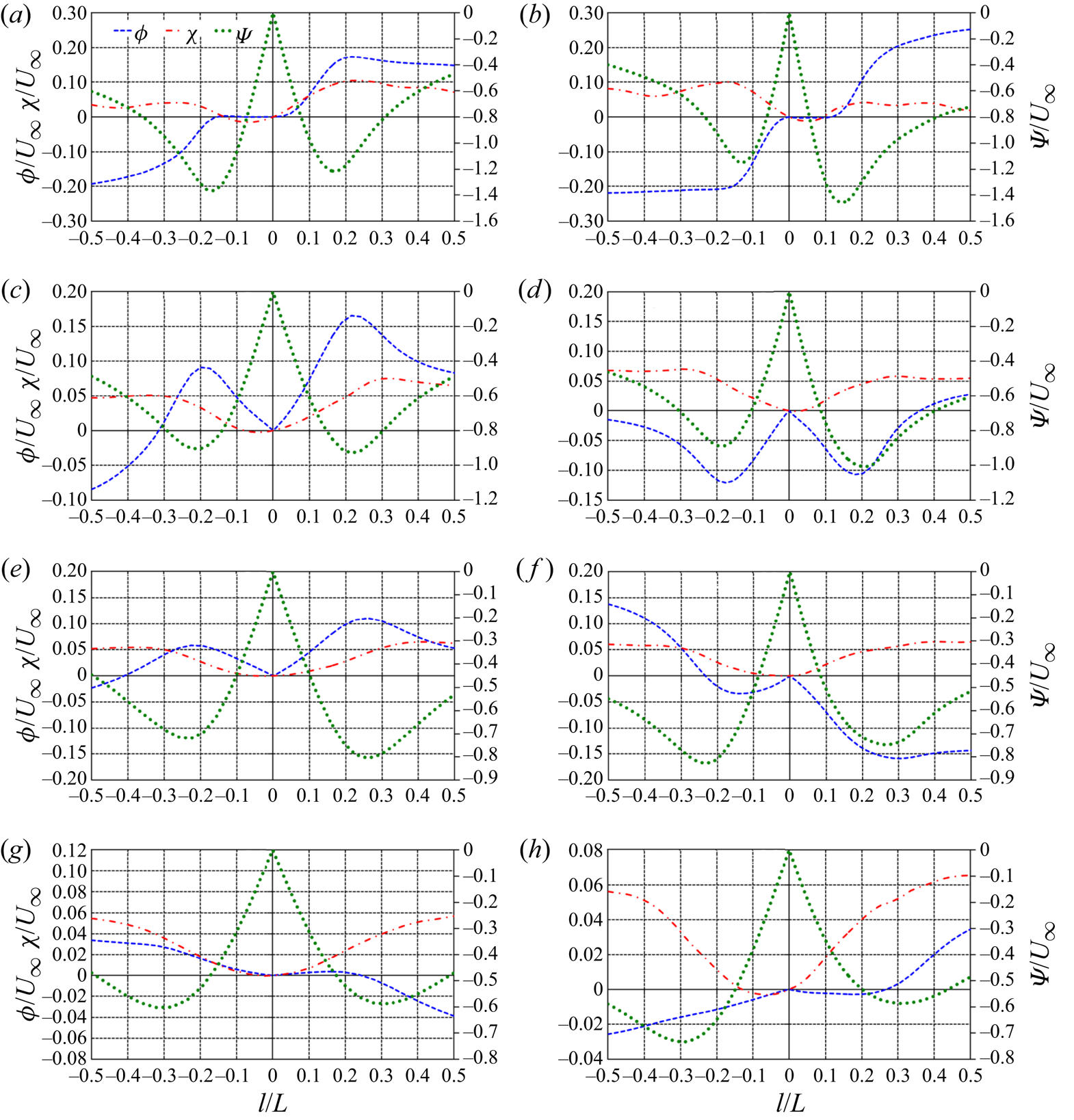
Velocity profiles across the tip vortices are reported in figure 17. In particular, the four vortices indicated by arrows in figure 16(c) were considered. The velocity profiles were extracted from the meridian slice of the phase-averaged field across the horizontal (streamwise) and vertical (radial) directions through the core of the tip vortices in the regions bounded by the isolines of pressure coefficient. All quantities in figure 17 are reported in a local reference frame centred at the vortex core, whose velocities were adopted to scale all values. The radial velocity,  $\phi$, was defined positive if directed away from the vortex core, while the tangential velocity,
 $\psi$, was defined positive for a counter-clockwise vortex. The axial velocity within the tip vortex,
 $\chi$, was assumed positive if directed outwards from the meridian plane. They were computed from the radial, azimuthal and axial velocity components within the cylindrical reference frame of the Eulerian grid,
 $u$,
 $v$ and
 $w$, respectively, taking into account the pitch angle of the tip vortex relative to the azimuthal direction, roughly equal to
 $6^{\circ }$. In figure 17 the profiles on the left were extracted along the direction of the
 $z$ coordinates, those on the right along the direction of the
 $r$ coordinates, to provide a glimpse of their variability within the tip vortices across the local tangential coordinate relative to the vortex core.
On the left and right sides, phase-averaged velocity profiles across the horizontal (streamwise) and vertical (radial) directions through the core of the tip vortices indicated in figure 16(c) as A (panels a and b), B (panels c and d), C (panels e and f) and D (panels g and h):  $\phi$,
 $\chi$ and
 $\psi$ for the radial, axial and tangential velocities, in the local reference frame centred at the vortex core,
 $l$ for the distance from the vortex core and
 $L$ for the local size of the vortex, bounded by the isolines of pressure in figure 16(c).

At the location A (see panels a and b of figure 17) the tangential velocity,  $\psi$, although not exactly symmetric relative to the vortex core, follows closely the behaviour of a Rankine vortex. This is not the case for the radial velocity,
 $\phi$, which is equal to zero in the inner region of the vortex, but experiences significant positive values in the outer region. This result highlights that the vortex core is expanding, as also pointed out by the isolines of pressure coefficient reported in figure 16. Overall, it appears that a Rankine model is better suited than the more sophisticated Batchelor model to represent the behaviour of the tip vortex in A. It should be also noted that in the adopted reference frame the axial velocity,
 $\chi$, is rather small, but in the reference frame of the rotor the latter is actually moving across the azimuthal direction with a speed roughly equal to
 $5.5U_\infty$.
Moving downstream at the location B (see panels c and d of figure 17) the evolution of the tangential velocity,  $\psi$, remains well represented by the Rankine vortex model, becoming also more symmetric. Instead, the radial velocity,
 $\phi$, moves farther away from the Rankine and Batchelor assumptions, although it is still an order of magnitude lower than
 $\psi$. It is also interesting to notice that, while on the left panel
 $\phi$ is positive, the opposite occurs on the right one. This indicates that the cross-section of the vortex is deviating from the circular shape, which is likely the result of the shear occurring with the surrounding structures populating the overall wake. As shown at the locations C (see panels e and f of figure 17) and D (see panels g and h of figure 17), the behaviour of the velocity profiles at the boundaries of the vortex becomes smoother as it moves downstream, which may be interpreted as a signature of the increasing instability of the tip vortices, resulting in higher levels of diffusion of the phase-averaged statistics. Nonetheless, the profile of tangential velocity,
 $\psi$, is still rather consistent with the Rankine assumption. As the tip vortices move downstream, the radial velocity,
 $\phi$, declines significantly, while the profile of velocity
 $\chi$, directed across their axis, is almost unchanged.
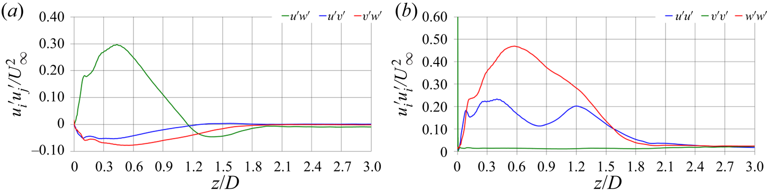
More details are provided in figure 18. In figure 18(a) for each streamwise location downstream of the turbine the phase-averaged values of the shear stresses at the core of the tip vortices were extracted. It should be noted that they were averaged across the tip vortices shed from the three blades of the turbine. The focus is on the near wake, where the instability of the tip vortices develops. The shear stresses are initially dominated by positive values of  $\widehat {u'w'}$, originating from the vorticity roll-up between the pressure and the suction sides of the blades of the turbine at their tip. It is clear that a dramatic change of the flow physics occurs starting at
 $z/D \approx 0.5$, where the development of a negative peak of
 $\widehat {u'w'}$ begins, which is achieved at
 $z/D \approx 1.4$. This result provides a confirmation that the shear stress
 $\widehat {u'w'}$ plays a major role in the process of destabilization of the tip vortices, through the interaction of each tip vortex with the wake of the preceding blade. In contrast,
 $\widehat {u'v'}$ and
 $\widehat {v'w'}$ reach a negative peak at the same streamwise location of the positive peak of
 $\widehat {u'w'}$, within the wake region where the tip vortices are still very coherent and their trajectory rather stable. Then, both
 $\widehat {u'v'}$ and
 $\widehat {v'w'}$ decline, as the coherence of the tip vortices is lost, showing a behaviour qualitatively different from that of
 $\widehat {u'w'}$.
Streamwise evolution within the near wake of the turbine of the phase-averaged shear (a) and normal (b) Reynolds stresses at the core of the tip vortices. Averages across the vortices shed by the three blades of the turbine.

The streamwise evolution across the near wake for the normal Reynolds stresses at the core of the tip vortices is shown in figure 18(b). It is initially dominated by the fluctuations of the streamwise velocity component, achieving a peak that roughly correlates with those of the shear stresses in (a). Then,  $\widehat {w'w'}$ starts a monotonic decrease. The behaviour by
 $\widehat {u'u'}$ is more complex, showing actually two maxima. The second one is obviously associated with the negative peak of
 $\widehat {u'w'}$, thus to the shear occurring between the tip vortices and the outer vorticity layer shed from the preceding blade. Actually, the signature of such an interaction in the streamwise evolution of the normal stresses is visible also for
 $\widehat {w'w'}$, whose negative slope experiences a decrease (in magnitude) in the same area where
 $\widehat {u'u'}$ develops its second peak. It is clear that instead
 $\widehat {v'v'}$ at the core of the tip vortices keeps a marginal role across the whole near wake of the turbine.
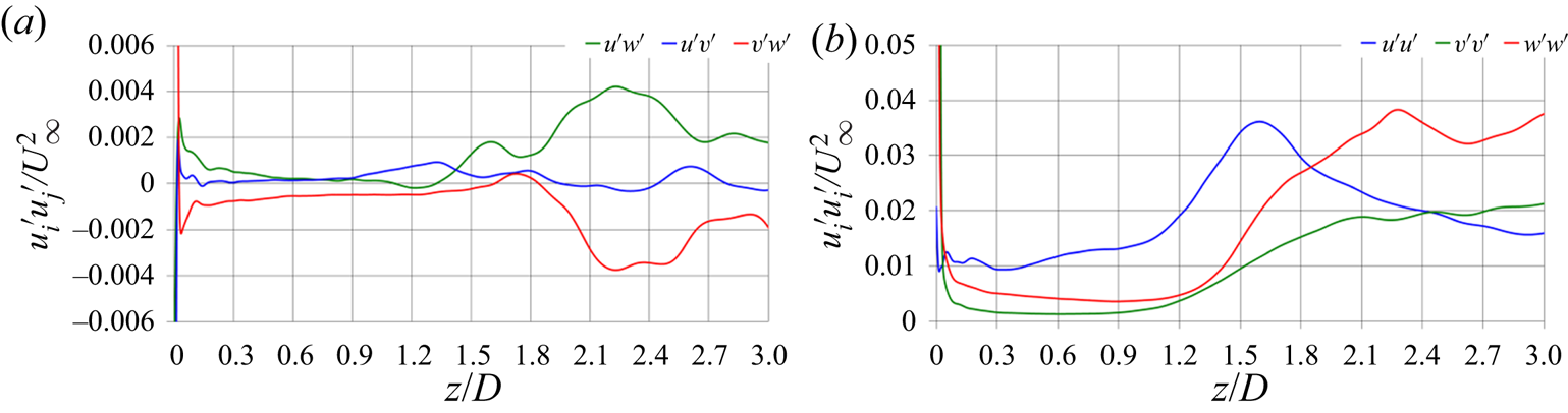
A similar analysis was carried out considering also a Lagrangian approach. From the instantaneous solutions of the flow, the core of the three tip vortices was identified at each streamwise location downstream of the rotor plane, again by means of local minima of pressure. Then, the Reynolds stresses were computed at the core of the tip vortices from the instantaneous values of the three velocity components. They are reported in figure 19. The results differ substantially from those presented in figure 18. First, they show much lower values across the whole streamwise evolution of the near wake. This result indicates that a significant contribution to the phase-averaged Reynolds stresses in figure 18, computed using an Eulerian approach, is due to the fluctuations of the trajectory of the tip vortices. Although very small, they occur even just downstream of the rotor plane, within a flow region where gradients are very sharp. Second, while the Reynolds stresses in figure 19 are very large when the tip vortices are generated, within the near wake they are much smaller and almost constant. They start growing only when the instability of the wake system fully develops. Third, this process of growth is delayed, compared with that observed in figure 18. In particular, as discussed above, in figure 18 the signature of the instability process is represented by the change of the slope of the streamwise evolution of the  $\widehat {u'w'}$ shear stress, occurring much earlier than the increase seen for all Reynolds stresses in figure 19. This provides confirmation that the increasing deviations from the helical trajectory of the tip vortices, due to short-wave and long-wave instabilities and then to mutual inductance between tip vortices, resulting in the rise of the phase-averaged Reynolds stresses within the Eulerian reference frame, are the trigger of the instability process and the increase of turbulence levels. They anticipate and eventually cause an increase of the velocity fluctuations within the core of the meandering tip vortices, as shown in figure 19, where they are associated with phenomena of small-scale turbulence.
Streamwise evolution within the near wake of the turbine of the shear (a) and normal (b) Reynolds stresses, computed at the core of the tip vortices using a Lagrangian approach. Averages across the vortices shed by the three blades of the turbine.

4.5. Correlation between instability and turbulence production
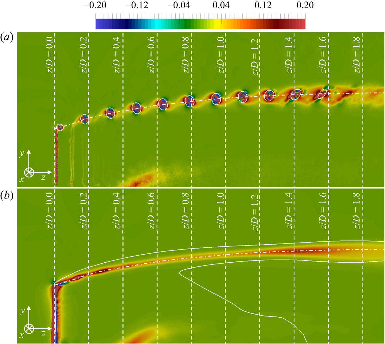
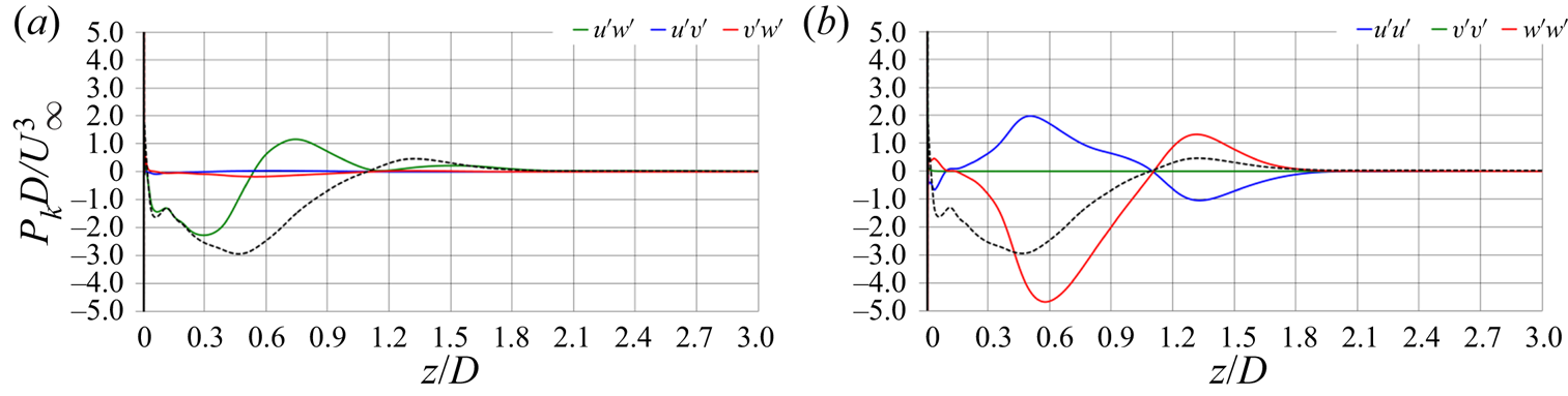
Turbulence production,  $P_k$, is also analysed in this section, with the purpose of a more accurate characterization of the areas where the instability is triggered and for comparison with the results of a similar analysis on the wake of a wind turbine, conducted by Lignarolo et al. (Reference Lignarolo, Ragni, Scarano, Simão Ferreira and Van Bussel2015) using PIV measurements. Figure 20 shows phase-averaged (a) and ensemble-averaged (b) contours of turbulence production up to the instability of the tip vortices. Figure 20(a) points to the presence of areas of both large positive and negative turbulence production within the tip vortices. In the outer region of the shear layer shed by each blade, production is always positive, reaching its maxima in the areas of shear with the tip vortices. Its values grow as the wake develops downstream, gradually affecting wider areas, including the core of the tip vortices. This behaviour is actually very similar to that observed for
 $\widehat {u'w'}$, providing additional evidence of its special role in leading to the destabilization of the wake system, via the shear originated by the roll up process of each tip vortex with the wake of the preceding blade. Similar results were reported in the experimental study by Lignarolo et al. (Reference Lignarolo, Ragni, Scarano, Simão Ferreira and Van Bussel2015), who also found both negative and positive peaks of
 $\hat {P}_k$ at the core of the tip vortices, connected between each others by regions of shear resulting in positive values of turbulence production. Figure 20(b) demonstrates that, although areas of negative production occur within the core of the tip vortices, as shown by the top panel,
 $\bar {P}_k$ is globally positive, showing the presence of a local peak at approximately
 $z/D=1.4$, again in agreement with the streamwise evolution observed above for
 $\overline {u'w'}$.
Phase-averaged (a) and ensemble-averaged (b) contours of turbulence production on a meridian plane through the axis of the turbine. Isolines for a value of the pressure coefficient  $\hat {c}_p=\bar {c}_p=-0.4$. The dotted-dashed line in both panels shows the ensemble-averaged trajectory of the tip vortices. Values of turbulence production scaled by
 $U_\infty ^{3}/D$.

The streamwise evolution of turbulence production was extracted at the core of the tip vortices from the phase-averaged fields. Their trajectory is illustrated by a dotted-dashed line in figure 20. Figures 21(a) and 21(b) report the contributions from the shear and normal Reynolds stresses, respectively. In both panels of figure 21 the dashed line represents the streamwise evolution of the overall production. Figure 21 illustrates that: (i) at the core of the tip vortices, production is mainly negative within the near wake, especially because of the contribution of  $\widehat {w'w'}$, balanced only in part by that of
 $\widehat {u'u'}$; (ii) the correlation between the evolution of
 $\hat {P}_k$ and
 $\widehat {u'w'}$ is weak, which is only seemingly in contrast with the results discussed above, where it was verified that the shear stress
 $\widehat {u'w'}$ grows as the instability of the tip vortices develops. Actually, the behaviour in figure 21, where values were extracted at the core of the tip vortices from phase-averaged statistics, just highlights that the main area of turbulence production within the near wake of the turbine, where instability grows, is not the core of the tip vortices, but instead the region between them, where shear contributes more substantially to positive production. This point is illustrated in more detail by the comparison between the results in figures 21 and 22. While the former were computed in an Eulerian reference frame, the latter were extracted at the core of the tip vortices in a Lagrangian reference frame. As reported above for the Reynolds stresses: (i) values in figure 22 are much lower than in figure 21, since most production comes from the large-scale fluctuations due to oscillations of the trajectory of the tip vortices around the mean helix; (ii) values in figure 22 start growing only once the instability of the wake system is triggered, producing small-scale turbulence at the core of the tip vortices, confirming that the original source of the instability process is not located within the core of the tip vortices, but rather in the region of mutual interaction between spirals.
Streamwise evolution within the near wake of the turbine of the phase-averaged turbulence production from the shear (a) and normal (b) Reynolds stresses at the core of the tip vortices. Averages across the vortices shed by the three blades of the turbine. The dashed line in both panels represents the overall turbulence production. The solid lines represent the contribution by each Reynolds stress.

Streamwise evolution within the near wake of the turbine of the time-averaged turbulence production from the shear (a) and normal (b) Reynolds stresses, computed at the core of the tip vortices using a Lagrangian approach. Averages across the vortices shed by the three blades of the turbine. The dashed line in both panels represents the overall turbulence production. The solid lines represent the contribution by each Reynolds stress.

To shed more light on the behaviour of turbulence production, the streamwise evolution of  $\hat {P}_k$ was investigated following an approach similar to that adopted by Lignarolo et al. (Reference Lignarolo, Ragni, Scarano, Simão Ferreira and Van Bussel2015) to analyse their PIV measurements on a meridian plane through the wake of a wind turbine. Actually, in the present case we have the possibility to exploit the whole azimuthal extent of the wake, with the purpose of increasing the size of the statistical sample. At each streamwise location the integral value of
 $\hat {P}_k$ was computed from the whole phase-averaged field as
 \begin{equation} IP_k (z) = \frac{D }{A U_\infty^{3}} \int_{r=0}^{r=R_b} {\int_{\vartheta=0}^{\vartheta=2 {\rm \pi}} {\hat{P}_k (r,\vartheta,z) \,\textrm{d}\vartheta\,\textrm{d}r}}, \end{equation}
where the integration was carried out within a radius  $r=R_b=D$. This way, taking into account the expansion of the wake, all important areas of large turbulence production are included. In (4.9), the quantity
 $A$ was selected as the area swept by the rotor,
 $A={\rm \pi} D^{2}/4$, rather than as the area of integration, in order to make the result from (4.9) independent from the choice of
 $R_b$, as long as the latter is large enough to include the whole wake of the turbine.
Figure 23 shows the streamwise evolution of  $IP_k$, which includes also the contribution to turbulence production by the region of shear between tip vortices (note that production from the inner radii at each cross-section of the wake is negligible): (i) the overall production is positive across the whole near wake; (ii) the peak of
 $IP_k$ is again located where the tip vortices develop mutual inductance, at
 $z/D\approx 1.4$; (iii) the main contribution to
 $IP_k$ up to the instability of the tip vortices at
 $z/D \approx 1.4$ comes from the shear stress
 $\widehat {u'w'}$; (iv) downstream of
 $z/D \approx 1.4$, turbulence production is dominated by
 $\widehat {u'w'}$, with almost no contribution from all other Reynolds stresses. The results in figure 23 confirm that the
 $\widehat {u'w'}$ shear stress developing at the outer boundary of the wake between tip vortices is the major source of turbulence, enhancing the process of wake instability. It should be noted that the agreement with the conclusions from the analysis conducted by Lignarolo et al. (Reference Lignarolo, Ragni, Scarano, Simão Ferreira and Van Bussel2015) is very satisfactory in terms of points (i) and (ii) above. In addition, the results of the present study allow us to distinguish the role of each Reynolds stress, regarding points (iii) and (iv), which was not investigated by them.
Streamwise evolution within the near wake of the turbine of phase-averaged turbulence production from the shear (a) and normal (b) Reynolds stresses. Integral values within cross-sections of the wake, based on (4.9). The dashed line in both panels represents the overall turbulence production. The solid lines represent the contribution by each Reynolds stress.

Following the same approach by Lignarolo et al. (Reference Lignarolo, Ragni, Scarano, Simão Ferreira and Van Bussel2015) the phase-averaged turbulence production was also decomposed into two different terms
 \begin{equation} \hat{P}_k ={-} \widehat{u_i'u_j'} \frac{\partial \hat{u}_i }{\partial x_j} ={-} \widehat{u_i'u_j'} \frac{\partial \bar{u}_i }{\partial x_j} - \widehat{u_i'u_j'} \frac{\partial \langle \hat{u}_i \rangle }{\partial x_j} = \hat{P}_k^{e} + \hat{P}_k^{p}, \end{equation}
where  $\langle \hat {u}_i \rangle =\hat {u}_i-\bar {u}_i$ is the deviation of the phase average from the ensemble average. As discussed by Lignarolo et al. (Reference Lignarolo, Ragni, Scarano, Simão Ferreira and Van Bussel2015),
 $P_k^{e}$ represents the decay into turbulence of the mean-flow kinetic energy, whereas
 $P_k^{p}$ correlates with the decay of the coherence of the periodic wake structures, which are mainly the tip vortices in the present flow. For both quantities the integral values over the cross-sections of the wake,
 $IP_k^{e}$ and
 $IP_k^{p}$ respectively, can be computed in a way similar to
 $IP_k$ in (4.9)
 \begin{gather} IP_k^{e} (z) = \frac{D }{A U_\infty^{3}} \int_{r=0}^{r=R_b} {\int_{\vartheta=0}^{\vartheta=2 {\rm \pi}} {\hat{P}_k^{e} (r,\vartheta,z) \,\textrm{d}\vartheta\,\textrm{d}r}}, \end{gather}
 \begin{gather} IP_k^{p} (z) = \frac{D }{A U_\infty^{3}} \int_{r=0}^{r=R_b} {\int_{\vartheta=0}^{\vartheta=2 {\rm \pi}} {\hat{P}_k^{p} (r,\vartheta,z) \,\textrm{d}\vartheta\,\textrm{d}r}}. \end{gather}
Figure 24 shows the streamwise evolution of  $IP_k^{e}$. A peak is produced at
 $z/D\approx 1.4$, due to mutual inductance and leapfrogging between tip vortices, increasing the levels of shear at the outer radii, as demonstrated by the contribution from
 $\widehat {u'w'}$. The tip vortices lose their synchronization with the rotation of the turbine and their instability starts the process of mixing between the wake core and the outer free stream. As a consequence, downstream of the peak at
 $z/D\approx 1.4$,
 $IP_k^{e}$ maintains large values. The streamwise evolution of
 $IP_k^{e}$ is mainly affected by the shear stress
 $\widehat {u'w'}$. Upstream of the instability of the tip vortices it comes from their mutual inductance, while more downstream it occurs at the shear layer between the wake region and the surrounding free stream at outer radii.
Streamwise evolution within the near wake of the turbine of phase-averaged turbulence production from the shear (a) and normal (b) Reynolds stresses. Integral values  $IP_k^{e}$ within cross-sections of the wake, based on (4.11). The dashed line in both panels represents the overall turbulence production. The solid lines represent the contribution by each Reynolds stress.

The behaviour of  $IP_k^{p}$ within the near wake is shown in figure 25. It is higher than
 $IP_k^{e}$ as long as the tip vortices remain very coherent and synchronized with the rotation of the turbine, while it goes almost to zero at
 $z/D\approx 1.4$, where coherence and synchronization are lost. Also in figure 25 turbulence production comes mainly from
 $\widehat {u'w'}$. Once again, the close agreement with the results by Lignarolo et al. (Reference Lignarolo, Ragni, Scarano, Simão Ferreira and Van Bussel2015) in showing the dominant role of
 $IP_k^{p}$ over
 $IP_k^{e}$ across the near wake of the turbine and its quick decline, due to the instability of the tip vortices, reinforces confidence in the accuracy of the simulations. Meanwhile, the availability of all components of the Reynolds stress tensor across the full azimuthal extent of the wake allowed us to distinguish their different contributions to turbulent production and identify the underlying flow physics. Production of turbulence is dominated by the shear stress
 $\widehat {u'w'}$ both upstream and downstream of the instability of the system of tip vortices, although its source is substantially different within the near wake and further away from the turbine. Upstream, it is mainly due to the shear occurring between the neighbouring helices of the tip vortices, through the ‘bridge’ represented by the shear layer populating the wake of each blade. Downstream, it is dominated by turbulent mixing, developing at the outer boundary of the wake between the lower-momentum fluid at inner radii and the free stream flow at outer radii when the process of wake contraction is triggered by instability phenomena.
Streamwise evolution within the near wake of the turbine of phase-averaged turbulence production from the shear (a) and normal (b) Reynolds stresses. Integral values  $IP_k^{p}$ within cross-sections of the wake, based on (4.12). The dashed line in both panels represents the overall turbulence production. The solid lines represent the contribution by each Reynolds stress.

5. Conclusions
LES on a cylindrical grid composed of approximately 1.9 billion points was utilized to capture the process of destabilization of the system of the tip vortices shed by an axial-flow turbine. The parameters of global performance were found to be in close agreement with those reported by Gaurier et al. (Reference Gaurier, Germain, Facq, Johnstone, Grant, Day, Nixon, Di Felice and Costanzo2015), who carried out a Round Robin experimental study on a similar turbine model. In addition, a good level of agreement was found with experimental studies in the literature on the wake of axial-flow hydrokinetic and wind turbines (Sherry et al. Reference Sherry, Nemes, Lo Jacono, Blackburn and Sheridan2013; Hong et al. Reference Hong, Toloui, Chamorro, Guala, Howard, Riley, Tucker and Sotiropoulos2014; Lignarolo et al. Reference Lignarolo, Ragni, Krishnaswami, Chen, Simão Ferreira and van Bussel2014, Reference Lignarolo, Ragni, Scarano, Simão Ferreira and Van Bussel2015; Lust et al. Reference Lust, Flack and Luznik2018, Reference Lust, Flack and Luznik2020) and marine propellers (Di Felice et al. Reference Di Felice, Di Florio, Felli and Romano2004; Felli et al. Reference Felli, Guj and Camussi2008, Reference Felli, Camussi and Di Felice2011), where similar phenomena of instability of the tip vortices develop. No earlier numerical computations were able to capture such phenomena with a level of detail similar to that reported in this study. The agreement with the experiments in the literature, besides providing confidence in the accuracy of the results, highlights the universality of the phenomena observed in the framework of the present study within the considered class of flows. They are indeed shared across axial-flow turbines and propellers having different geometrical features and working conditions.
Thanks to the time-accurate methodology, instantaneous realizations of the solution provided details on the development of instability, reproducing the phenomena observed in the experiments by Felli et al. (Reference Felli, Camussi and Di Felice2011) for the wake of a notional marine propeller. The helical trajectory of the tip vortices was initially very stable. However, both short-wave and long-wave instabilities around the mean helix gradually developed, increasing in amplitude across the streamwise direction away from the turbine. These oscillations promoted mutual inductance between tip vortices, leading to vortex meandering, pairing and leapfrogging, thus enhancing the deviation of the tip vortices from their original helical trajectory and amplifying the process of their destabilization. Eventually, the tip vortices break down into smaller structures, losing their large-scale coherence and producing a wide region of diffused turbulent stresses at the outer radii of the wake, initiating the process of wake contraction and momentum recovery via turbulent mixing, as discussed by Lignarolo et al. (Reference Lignarolo, Ragni, Krishnaswami, Chen, Simão Ferreira and van Bussel2014, Reference Lignarolo, Ragni, Scarano, Simão Ferreira and Van Bussel2015) for the wake of a wind turbine.
The present dataset allowed us to focus our analysis on the behaviour of shear stresses and turbulence production through a detailed vortex core analysis. Increasing levels of turbulent shear stress associated with the fluctuations of the radial and axial velocity components were observed to affect the outer radii of the wake, due to the shear produced between each tip vortex and the outer region of the shear layer shed from the trailing edge of the preceding blade. Turbulence production was indeed verified to be especially large, not within the core of the tip vortices, but in the region between them where mutual inductance developed. This conclusion was also confirmed by the comparisons of both Reynolds stresses and turbulence production computed via Eulerian and Lagrangian approaches, respectively. The interaction between helices was promoted by the larger pitch of the tip vortices, compared with the wake shed by each blade of the turbine, resulting in a faster advancement across the streamwise direction away from the rotor plane. These phenomena produced a ‘bridge’ between consecutive tip vortices and promoted mutual inductance between them, amplifying the oscillations of their helical trajectory and resulting in maxima of turbulent production. They were due first to the large-scale fluctuations, associated with the meandering of the tip vortices, and then to the small-scale turbulence developing at the core of the tip vortices as a result of their instability.
The present results, dealing with the ability of the shear between tip vortices and the wake of the neighbouring blades to trigger the wake instability, never reported in earlier studies dealing with axial-flow turbines, provide a confirmation of the hypothesis formulated by Di Felice et al. (Reference Di Felice, Di Florio, Felli and Romano2004) and Felli et al. (Reference Felli, Guj and Camussi2008, Reference Felli, Camussi and Di Felice2011) for marine propellers. They observed in their experiments an earlier onset of wake instability at higher loads and with propeller geometries consisting of more blades, resulting in smaller inter-spiral distances and in a faster development of mutual inductance phenomena between tip vortices. In particular, in the present case, this result was made more evident by the marginal role of the hub vortex, making it easier to isolate the importance of the shear between the tip vortices and the vorticity sheet populating the wake of the neighbouring blades in the process of instability.
Acknowledgements
We acknowledge PRACE for awarding us access to Joliot Curie KNL at GENCI/CEA, France, with an allocation granted to the project ‘wakehydroLES – Characterization of the wake of an axial-flow hydrokinetic turbine via LES’ (project no. 2019204935) in the framework of the 19th PRACE Call for Proposals for Project Access.
Declaration of interests
The authors report no conflict of interest.