1. Introduction
In fluid mechanics, investigating the flow around blunt bodies is crucial for understanding fluid behaviour and optimising engineering designs. As a canonical blunt body, the sphere has received considerable attention due to its broad applications in aerospace, marine engineering and sports equipment design (Seifert Reference Seifert2012; Goff Reference Goff2013; Alam, Chowdhury & Moria Reference Alam, Chowdhury and Moria2019; Derakhshandeh & Alam Reference Derakhshandeh and Alam2019; Shah, Shakya & Mittal Reference Shah, Shakya and Mittal2019; Ward et al. Reference Ward, Passmore, Spencer, Hanson and Lucas2023). The drag and lift of a sphere are critical indicators of its hydrodynamic performance, primarily determined by Reynolds number, shape and motion mode. Consequently, achieving significant drag reduction while maintaining low lift remains a major engineering challenge. Recently, researchers have investigated various drag-reduction strategies, including passive methods (e.g. pits, surface roughness, vortex generators) and active methods (e.g. fluid injection or suction), with notable success (Choi, Jeon & Kim Reference Choi, Jeon and Kim2008; Rashidi, Hayatdavoodi & Esfahani Reference Rashidi, Hayatdavoodi and Esfahani2016).
To provide a clear framework for the literature review and subsequent analysis, the geometric configuration is defined in figure 1, where
 $x,\ y$
and
 $z$
denote the longitudinal, lift and transverse directions, respectively.
1.1. Stationary sphere baseline
Although the sphere is a simple, highly symmetric three-dimensional structure, increasing Reynolds number triggers a sequence of wake flow mechanisms characterised by complex regime transitions. At very low Reynolds numbers (
 $Re \lt 1$
), viscous forces dominate, defining the creeping flow regime (Dennis & Walker Reference Dennis and Walker1971). As
 $Re$
increases to the range
 $1 \lt Re \lt 20$
, the fluid remains fully attached to the sphere surface, maintaining a stable laminar state. The first separation occurs at
 $Re \approx 20$
, initiating an axisymmetric regime with zero lift that persists up to
 $Re \approx 210$
(Taneda Reference Taneda1956). Tiwari et al. (Reference Tiwari, Pal, Bale, Minocha, Patwardhan, Nandakumar and Joshi2020) provided a comprehensive taxonomy of the subsequent states based on the prevailing flow physics, categorising the wake evolution into planar-symmetric, vortex-shedding, subcritical and critical regimes. Beyond
 $Re \approx 210$
, the wake dynamics is governed by the competition between global and shear-layer instabilities. The first instability arises at
 $Re \approx 210$
, causing the stationary vortex ring to deviate from the central axis and form a double-threaded wake (Magarvey & Bishop Reference Magarvey and Bishop1961; Nakamura Reference Nakamura1976). At
 $Re \approx 270$
, a second instability introduces a wavy, double-threaded pattern (Ormières & Provansal Reference Ormières and Provansal1999), followed by the periodic detachment of hairpin vortices at
 $Re \approx 300$
(Johnson & Patel Reference Johnson and Patel1999). Utilising principal spectrum analysis, Lu et al. (Reference Lu, Lin, Lin and Chang2024) identified that at
 $Re \in [390, 420]$
, the intensity and phase of these shedding vortices vary across successive events, with vorticity patterns rotating around the central axis in the near wake. Between
 $Re = 480$
and
 $650$
, these global instabilities dominate, leading to the irregular detachment of large-scale hairpin structures (Sakamoto & Haniu Reference Sakamoto and Haniu1990, Reference Sakamoto and Haniu1995) and the breaking of spatial symmetries. At
 $Re \approx 650$
, the flow enters the separating vortex tubes regime. The intense velocity gradients within the shear layer trigger pulsation behaviour, resulting in the formation of vortex tubes that develop shear-layer instability as they are carried downstream. While this transition is traditionally observed at
 $Re \approx 650$
(Mittal & Najjar Reference Mittal and Najjar1999), other studies suggest a slightly higher threshold of
 $Re \approx 800$
for the onset of this mechanism (Mittal, Wilson & Najjar Reference Mittal, Wilson and Najjar2002; Tiwari et al. Reference Tiwari, Bale, Patwardhan, Nandakumar and Joshi2019). This phenomenon persists up to
 $Re \approx 3000$
, beyond which the flow enters the subcritical regime (regime V,
 $3 \times 10^3 \leqslant Re \leqslant 3.4 \times 10^5$
). In this regime, the shear-layer instabilities increase linearly with
 $Re$
, as characterised by the
 $St$
–
 $Re$
relationship, while the drag coefficient remains nearly constant. Finally, as the Reynolds number reaches the critical regime (regime VI,
 $3.4 \times 10^5 \leqslant Re \leqslant 4.4 \times 10^5$
), the flow undergoes the well-known drag crisis. Using surface oil-flow and smoke visualisations across a wide range (
 $1 \times 10^4 \leqslant Re \leqslant 1 \times 10^6$
), Taneda (Reference Taneda1978) observed that the subcritical wake maintains its characteristic topology until
 $Re \approx 3.8 \times 10^5$
. At this juncture, a rapid drop in the drag coefficient is observed, reaching a minimum of
 $C_D \approx 0.1$
at
 $Re \approx 3.7 \times 10^5$
. This transition is marked by a sudden shrinkage of the recirculation region, triggered by the turbulent transition of the boundary layer prior to separation. This naturally occurring shear-layer instability within the subcritical regime is prominently showcased in the classic visualisations by Werlé (Reference Werlé1980) at
 $Re = 1.5 \times 10^4$
(see also Van Dyke Reference Van Dyke1982, p. 34). These foundational observations have been corroborated by the more recent experimental study of Jang & Lee (Reference Jang and Lee2007) at
 $Re = 1.1 \times 10^4$
. At these subcritical Reynolds numbers, qualitative dye and smoke visualisations consistently depict the organised roll-up of nearly symmetric vortex rings, representing a direct manifestation of the Kelvin–Helmholtz instability. This persistent physical evidence, observed across both classic and contemporary studies, establishes a robust framework for our current analysis at
 $Re = 1 \times 10^4$
. It confirms that the shear-layer instability remains the fundamental governing mechanism of the near-wake transition, providing a reliable baseline for interpreting how this instability is modulated or suppressed under the influence of surface rotation.
Schematic of a uniform flow (with velocity
 $U_\infty$
) past a rotating sphere with a stationary hood over the back half of the sphere. The rotating speed is
 $\varOmega$
and the rotating direction is along the negative
 $z$
axis.

Modifying the shape of a sphere can significantly alter its boundary layer and wake, thereby reducing drag. For pitted spheres, separation bubbles within the pits induce shear-layer instabilities, enhance turbulence intensity and transition the boundary layer from laminar to turbulent flow. This downstream shift of the separation point advances the drag crisis relative to a smooth sphere, reducing drag. Choi, Jeon & Choi (Reference Choi, Jeon and Choi2006) experimentally studied smooth and dimpled spheres at Reynolds numbers from
 $0.5 \times 10^5$
to
 $2.8 \times 10^5$
. Dimples with a depth of 0.6 mm and diameter of 13 mm allowed the boundary layer to remain laminar for smooth spheres, while achieving up to 50
 $\,\%$
drag reduction for dimpled spheres at
 $ Re \geqslant 9 \times 10^4$
. Aoki, Muto & Okanaga (Reference Aoki, Muto and Okanaga2012) further demonstrated that increasing dimple depth ratios (
 $k/D$
) enhances the reduction in the critical Reynolds number. Beratlis, Balaras & Squires (Reference Beratlis, Balaras and Squires2019) conducted direct numerical simulations (DNS) at subcritical (
 $10^4$
) and postcritical (
 $1.1 \times 10^5$
) Reynolds numbers, confirming approximately 50
 $\,\%$
drag reduction for dimpled spheres postcritical, while showing negligible effect at subcritical Reynolds numbers. Surface roughness has also been shown to influence drag. Achenbach (Reference Achenbach1974) studied spheres with surface roughness ratios
 $k/D$
ranging from 0.00025 to 0.01250 and
 $Re$
from
 $5 \times 10^4$
to
 $6 \times 10^6$
, finding that drag first decreases sharply and then increases, with the critical Reynolds number decreasing as roughness increases. Tang et al. (Reference Tang, Lu, Zhou, Gao, Lyu and Ke2024) used quasi-DNS to examine particle flow over surfaces with roughness from 0.011 to 10.847 μm, revealing that drag remains nearly constant for
 $Re \le 500$
, but decreases progressively at higher Reynolds numbers. Son et al. (Reference Son, Choi, Jeon and Choi2011) used surface trip wires with varying diameters and angles, achieving up to 60
 $\,\%$
drag reduction at corrected
 $Re$
of
 $1.5{-}1.7\times 10^5$
. Active control methods, such as periodic blowing and suction through surface slits (Jeon et al. Reference Jeon, Choi, Jeon, Choi and Park2004), can reduce drag by nearly 50
 $\,\%$
. Chae et al. (Reference Chae, Lee, Kim and Lee2019) developed an adaptive moving ring device, reducing drag by up to 74
 $\,\%$
for
 $Re$
ranging from
 $0.4\times 10^5$
to
 $4.4\times 10^5$
.
Parallel to these geometric modifications, active flow control strategies – most notably sphere rotation – have garnered significant attention due to their ability to directly inject momentum into the boundary layer. However, the resulting hydrodynamic mechanisms depend critically on the alignment of the rotation axis relative to the free stream.
1.2. Longitudinal rotation about the
 $x$
axis

Specifically, regarding rotation about the longitudinal axis, the rotation vector aligns parallel to the free stream. This configuration imparts a swirling motion to the flow, fundamentally altering the boundary-layer development and wake topology through centrifugal effects. Hoskin (Reference Hoskin1955) characterised the migration of the separation point with respect to the rotation speed, revealing that the separation line advances upstream towards the windward face as the rotation rate increases. This upstream shift extends the wake region, typically leading to a gradual increase in the drag coefficient (Luthander & Rydbergy Reference Luthander and Rydbergy1935; Schlichting & Gersten Reference Schlichting and Gersten2017). Furthermore, in the laminar regime, Kim & Choi (Reference Kim and Choi2002) investigated the flow stability and established that the wake instability is governed by the interplay between the Reynolds number and rotation rate. Their results demonstrated that longitudinal rotation significantly modifies the vortex-shedding characteristics and the topological structure of the near wake.
In contrast to the longitudinal case, rotation about the transverse axis fundamentally breaks the flow symmetry, leading to highly non-axisymmetric dynamics.
1.3. Transverse rotation about the
$z$
axis

When a sphere rotates transversely, pressure differences generate lift, altering its trajectory. If the lift aligns with
 $U_\infty \times \omega$
, it is referred to as the Magnus effect; if it opposes
 $U_\infty \times \omega$
, it is called the inverse Magnus effect. For low Reynolds numbers (
 $Re \ge 1$
), Rubinow & Keller (Reference Rubinow and Keller1961) derived
 $C_L = 2\alpha$
for the lift coefficient of a transversely rotating sphere, where
 $\alpha = \varOmega D / 2 U_\infty$
is the non-dimensional rotation rate. Experimental studies by Tsuji, Morikawa & Mizuno (Reference Tsuji, Morikawa and Mizuno1985) estimated
 $C_L = (0.40 \pm 0.10)\alpha$
for rotational speeds
 $\alpha \ge 0.7$
and
 $550 \leqslant Re \leqslant 1600$
, with further models summarised by Loth (Reference Loth2008). Beyond the variation of hydrodynamic coefficients, transverse rotation fundamentally modulates the wake topology and vortex-shedding dynamics. The interaction between the rotating surface and the separating shear layers induces complex flow instabilities that are distinct from the stationary case. Giacobello, Ooi & Balachandar (Reference Giacobello, Ooi and Balachandar2009) and Kim (Reference Kim2009) studied
 $Re = 100{-}300$
and extended rotational speeds up to
 $\alpha = 1.2$
, while Dobson, Ooi & Poon (Reference Dobson, Ooi and Poon2014) investigated up to
 $\alpha = 3$
. At
 $Re = 300$
, hairpin vortices shed periodically for
 $0 \leqslant \alpha \leqslant 0.3$
; shedding is suppressed and the wake stabilises into a double thread for
 $0.5 \leqslant \alpha \leqslant 0.6$
. Higher rotation induces shear-layer instabilities (
 $0.8 \leqslant \alpha \leqslant 2$
) and a separatrix regime (
 $2.5 \leqslant \alpha \leqslant 3$
), with drag first increasing and then decreasing with
 $\alpha$
. Additionally, Poon et al. (Reference Poon, Ooi, Giacobello, Iaccarino and Chung2014) identified a ‘shear layer-stable foci’ regime for
 $\alpha = 1$
at
 $Re = 500$
and for
 $0.8 \leqslant \alpha$
at
 $640 \leqslant Re \leqslant 1000$
. Kurose & Komori (Reference Kurose and Komori1999) found that drag increases with both rotation speed and shear strength for
 $Re = 1{-}500$
and
 $\alpha = 0{-}0.25$
. For higher Reynolds numbers under transverse rotation, the flow physics becomes increasingly complex due to the interplay between rotation and turbulence. Kim et al. (Reference Kim, Choi, Park and Yoo2014) reported that at
 $Re = 0.6{-}1.8 \times 10^5$
and
 $\alpha = 0{-}1.7$
, the mean drag and lift coefficients initially rise, then fall, and rise again. Low rotation speeds yield negative lift, indicating the inverse Magnus effect, caused by laminar–turbulent asymmetry in the boundary layer. Muto, Tsubokura & Oshima (Reference Muto, Tsubokura and Oshima2012) conducted large-eddy simulations (LES) of flow around a sphere at subcritical (
 $1.0 \times 10^4$
), critical (
 $2.0 \times 10^5$
) and supercritical (
 $1.14 \times 10^6$
) Reynolds numbers with varying rotation speeds
 $0 \leqslant \alpha \leqslant 1$
. At the critical Reynolds number, lift is negative at low rotation and becomes positive as rotation increases, whereas at sub- and supercritical regimes, lift increases monotonically with rotation. Li, Tsubokura & Tsunoda (Reference Li, Tsubokura and Tsunoda2017) simulated a golf ball (area ratio 0.005) and a smooth sphere, both rotating at 0.1, at
 $Re = 4.3 \times 10^4$
,
 $7.5 \times 10^4$
,
 $1.1 \times 10^5$
for the golf ball and
 $Re = 1.0 \times 10^4$
,
 $2.0 \times 10^5$
,
 $1.14 \times 10^6$
for the smooth sphere; both bodies show positive lift at sub- and supercritical regimes but negative lift at the critical Reynolds number; rotation decreases drag for the golf ball at
 $Re = 7.5 \times 10^4$
while increasing it elsewhere, and increases drag for the smooth sphere across all Reynolds numbers; the negative Magnus effect arises from asymmetric boundary-layer transition, with the top remaining laminar and the bottom turbulent, shifting flow separation downstream and producing negative lift.
Building upon our previous investigation of laminar flow (
 $Re = 200$
and 300) (Lu & Chang Reference Lu and Chang2025), the present study extends the strategy of simultaneous drag and lift reduction into the subcritical turbulent regime. To facilitate a comparative analysis, three configurations are considered: the flow past a stationary bluff body (SB), a fully rotating bluff body (RB) and a rotating bluff body shielded by a stationary hood over its rear half (RBH). The key idea revealed by force-element analysis (FEA; proposed by Chang (Reference Chang1992), and Chang, Yang & Chu (Reference Chang, Yang and Chu2008) for multiple bodies) is that drag can be significantly reduced by RBH. Meanwhile, half-rotation (with the rear half-sphere being stationary) effectively turns off or even reverses the Magnus effect, yielding a small lift, too. However, for the cylinder case, we achieve nearly zero lift
 $C_L$
at a critical
 $\alpha _I$
where we have zero drag
 $C_D$
, while for the sphere case,
 $C_L$
remains substantial (not close to zero) at the critical
 $\alpha _I$
where we have zero drag
 $C_D$
. This is because of the imbalance of volume-vorticity lift term (weaker
 $C_{LV}^+$
) and surface-vorticity lift term (stronger
 $C_{LS}^-$
) in the laminar flow. In the regime of turbulent flow (
 $Re = 1 \times 10^4$
, this study), it is expected that the volume-vorticity lift term increases in strength while the surface-vorticity lift term reduces its contribution to the lift, thus yielding a substantial simultaneous reduction of drag and lift. This study confirms this line of thought and is devoted to reporting the related findings and the detailed physical mechanisms of achieving this goal.
This paper is organised as follows: § 2 presents the physical problem and analysis methods, § 3 addresses the mechanisms of drag and lift reduction from the perspective of FEA and § 4 summarises the main conclusions.
2. The physical model and method of analysis
This section begins with a brief overview of FEA. This is followed by a description of the fundamental physical problem and numerical validation.
2.1. Force-element theory in turbulence based on delayed detached eddy simulation model
For flow past a rotating sphere at a subcritical Reynolds number (
 $Re = 1 \times 10^4$
), it is assumed that the fluid has a constant density
 $\rho$
and a dynamic viscosity
 $\mu$
. In order to present the results concisely in non-dimensional form, the sphere’s diameter
 $D$
is used as the reference length, the incoming velocity
 $U_\infty$
at infinity as the reference velocity, the ratio
 ${D}/{U_\infty }$
as the reference time and
 $\rho U_\infty ^2$
as the reference pressure. Let
 $\varOmega = 2 \pi f$
denote the angular speed of the sphere, where
 $f$
is the rotational frequency. For later use, we define
 $\alpha = {\varOmega D}/{2U_\infty }$
, the non-dimensional speed ratio. The incompressible turbulent flow induced by the motion of the sphere is governed by the continuity equation and the incompressible Reynolds-averaged Navier–Stokes (RANS) equation, expressed in dimensionless form as follows:
 \begin{equation} \boldsymbol{\nabla } \boldsymbol{\cdot }\bar {\boldsymbol{u}}=0 \end{equation}
and
 \begin{equation} \frac {\partial \bar {\boldsymbol{u}}}{\partial t}+\bar {\boldsymbol{u}} \boldsymbol{\cdot }\boldsymbol{\nabla } \bar {\boldsymbol{u}}=-\boldsymbol{\nabla } \bar {p} + \frac {1}{Re}{{\nabla} }^{2}\bar {\boldsymbol{u}}+\boldsymbol{\nabla } \boldsymbol{\cdot }\boldsymbol{\tau }. \end{equation}
Here
 $\bar {\boldsymbol{u}}$
and
 $\bar {p}$
represent the flow velocity and pressure, respectively, while
 $Re = \rho U_\infty D/ \mu$
denotes the Reynolds number. The last term
 $\boldsymbol{\nabla } \boldsymbol{\cdot }\boldsymbol{\tau }= {\partial \tau _{ij}}/{\partial x_{j}}$
on the right-hand side of the momentum equation represents the Reynolds stress term. In the delayed detached eddy simulation (DDES) turbulence model,
 $\tau _{ij,\ \textit{turbulent}}$
denotes the Reynolds stress tensor (Spalart et al. Reference Spalart, Deck, Shur, Squires, Strelets and Travin2006). The Boussinesq hypothesis (see Pope Reference Pope2000, p. 93), introduced by Joseph Boussinesq in 1877, is a key concept in turbulence modelling. It establishes the relationship between Reynolds stresses and mean velocity gradients, expressed in dimensionless form as follows:
 \begin{equation} \tau _{ij}=\tau _{ij,\ \textit{turbulent}}= \frac {1}{Re_t}\left(\frac {\partial \bar {u}_{i}}{\partial x_{j}}+\frac {\partial \bar {u}_{j}}{\partial x_{i}}\right)-\frac {2}{3}k\delta _{ij}. \end{equation}
Here,
 $Re_t=\rho U_\infty D/\mu _{t}$
, where
 $\mu _{t}$
represents the turbulence eddy viscosity, and
 $k$
denotes the turbulence kinetic energy. The vorticity,
 $\boldsymbol{\omega } = \boldsymbol{\nabla }\times \boldsymbol{u}$
, is another crucial quantity for subsequent analysis.
In most of the literature (see White & Xue Reference White and Xue2021, p. 317), the drag coefficient, the lift coefficient and the side-force coefficient are defined in terms of
 \begin{equation} C_{D}=\dfrac {F_{D}}{\dfrac {1}{2}\rho U_\infty ^2 A_0},\quad C_{L}=\dfrac {F_{L}}{\dfrac {1}{2}\rho U_\infty ^2 A_0}\quad \mbox{and} \ C_{S}=\dfrac {F_{S}}{\dfrac {1}{2}\rho U_\infty ^2 A_0}. \end{equation}
Note that
 $F_{D}$
,
 $F_{L}$
and
 $F_{S}$
stand for drag, lift and side-force, respectively, while
 $A_0={\pi D^2}/4$
denotes the projection area of the sphere. Each force component comprises two contributions: the pressure force, which originates from the normal stress distribution on the surface, and the skin-friction force, which arises due to the tangential shear stress. The directions of drag, lift and side-force are denoted by
 $\boldsymbol{i}$
,
 $\boldsymbol{j}$
and
 $\boldsymbol{k}$
, respectively.
Let
 $\boldsymbol{n}$
denote the unit normal vector on the body surface, pointing towards the inside of the sphere. Since the three-dimensional definitions of the drag coefficient
 $C_{D}$
, the lift coefficient
 $C_{L}$
and the side-force coefficient
 $C_{S}$
for the sphere include a factor of
 $\pi$
, these coefficients can be expressed as
 \begin{equation} \gamma C_{D}=\int _{S_{0}}\bar {p}(\boldsymbol{n}\boldsymbol{\cdot }\boldsymbol{i})\mathrm{d}A+\frac {1}{Re}\int _{S_{0}}(\boldsymbol{n}\times \bar {\boldsymbol{\omega }})\boldsymbol{\cdot }\boldsymbol{i}\mathrm{\,d}A, \end{equation}
 \begin{equation} \gamma C_{L}=\int _{S_{0}}\bar {p}(\boldsymbol{n}\boldsymbol{\cdot }\boldsymbol{j})\,\mathrm{d}A+\frac {1}{Re}\int _{S_{0}}(\boldsymbol{n}\times \bar {\boldsymbol{\omega }})\boldsymbol{\cdot }\boldsymbol{j}\mathrm{\,d}A \end{equation}
and
 \begin{equation} \gamma C_{S}=\int _{S_{0}}\bar {p}(\boldsymbol{n}\boldsymbol{\cdot }\boldsymbol{k})\mathrm{d}A+\frac {1}{Re}\int _{S_{0}}(\boldsymbol{n}\times \bar {\boldsymbol{\omega }})\boldsymbol{\cdot }\boldsymbol{k}\mathrm{\,d}A. \end{equation}
Note that the additional term arising from
 $(\boldsymbol{\tau }\boldsymbol{\cdot }\boldsymbol{n})$
vanishes on the body surface, as the DDES model employs the Boussinesq approximation for turbulence modelling. Here,
 $\gamma =\pi /8$
and
 $S_{0}$
represents the surface of the sphere.
Distributions of the auxiliary potentials (a)
 $\phi _i$
, (b)
 $\phi _j$
and (c)
 $\phi _k$
around the sphere, defined by (2.8)–(2.11), (2.18)–(2.20) and (2.23)–(2.25), respectively. The contours are displayed on slices at
 $z = \pm 0.4$
,
 $\pm 0.3$
,
 $\pm 0.2$
and
 $0$
. The visualisation includes the symmetry plane
 $z = 0$
and the semi-sphere surface for
 $z \leqslant 0$
.

In this study, an alternative approach to obtain the drag coefficient
 $C_D$
in (2.5) is to use the FEA method proposed by Chang (Reference Chang1992). As part of the derivation process, an auxiliary potential function
 $\phi _i$
is introduced, which physically represents the potential flow generated by the motion of the sphere with unit velocity in the negative drag direction. This potential
 $\phi _i$
is governed by the Laplace equation
 \begin{equation} {\nabla} ^{2}\phi _{i}=0, \end{equation}
and boundary conditions
 \begin{equation} \boldsymbol{\nabla }\phi _{i}\boldsymbol{\cdot }\boldsymbol{n}=-\boldsymbol{i}\boldsymbol{\cdot }\boldsymbol{n}, \quad \boldsymbol{r} \; \mbox{on} \; S_{0}, \end{equation}
 \begin{equation} \phi _{i}=0,\quad \boldsymbol{r} \rightarrow \infty . \end{equation}
In this study, we have numerically solved (2.8) within the domain
 $V_R$
. The external surface of the control volume
 $V_R$
is denoted as
 $S_R$
. The outer boundary
 $S_R$
is assumed to be sufficiently distant from the sphere, allowing (2.10) to be approximated as
 \begin{equation} \phi _{i}=0,\quad \boldsymbol{r} \; \mbox{on} \; S_{R}, \; \mbox{as} \; R \rightarrow \infty . \end{equation}
Figure 2(a) presents a detailed view of
 $\phi _{i}$
around the sphere in this study. Similar physical interpretations apply to the auxiliary potentials in the lift (
 $\phi _j$
) and side-force (
 $\phi _k$
) directions. As visualised in figure 2, the spatial distributions of these three potentials play a critical role in the force-element decomposition, acting as the weighting fields that extract specific force components from the complex flow field. The two vector identities
 \begin{equation} \bar {\boldsymbol{u}}\boldsymbol{\cdot }\boldsymbol{\nabla }\bar {\boldsymbol{u}}=\frac {1}{2}\boldsymbol{\nabla }|\bar {\boldsymbol{u}}|^{2}-\bar {\boldsymbol{u}}\times \bar {\boldsymbol{\omega }} \end{equation}
and
 \begin{equation}{\nabla} ^{2}\bar {\boldsymbol{u}}=\boldsymbol{\nabla }(\boldsymbol{\nabla }\boldsymbol{\cdot }\bar {\boldsymbol{u}})-\boldsymbol{\nabla }\times \bar {\boldsymbol{\omega }}=-\boldsymbol{\nabla }\times \bar {\boldsymbol{\omega }} \end{equation}
are used to rewrite the advective and viscous terms in (2.2). In this case, the corresponding momentum equation is written as
 \begin{equation} -\boldsymbol{\nabla }\bar {p} =\frac {\partial \bar {\boldsymbol{u}}}{\partial t}+\frac {1}{2}\boldsymbol{\nabla }|\bar {\boldsymbol{u}}|^2-\bar {\boldsymbol{u}}\times \bar {\boldsymbol{\omega }}+\frac {1}{Re}(\boldsymbol{\nabla }\times \bar {\boldsymbol{\omega }})-\boldsymbol{\nabla } \boldsymbol{\cdot }\boldsymbol{\tau }. \end{equation}
By taking the inner product with
 $\boldsymbol{\nabla }\phi _i$
on both sides of (2.14) within the control volume
 $V_R$
, utilising (2.2) and applying the Gauss divergence theorem, we derive
 \begin{eqnarray} \int _{S_{0}}\bar {p}(\boldsymbol{n}\boldsymbol{\cdot }\boldsymbol{i})\mathrm{\,d}A & = & \int _{S_{0}}\phi _{i}\frac {\partial \bar {\boldsymbol{u}}}{\partial t}\boldsymbol{\cdot }\boldsymbol{n}\mathrm{\,d}A -\frac {1}{2}\int _{S_{0}}|\bar {\boldsymbol{u}}|^{2}\boldsymbol{n}\boldsymbol{\cdot }\boldsymbol{i}\mathrm{\,d}A- \int _{V_{R}}\bar {\boldsymbol{u}}\times \bar {\boldsymbol{\omega }} \boldsymbol{\cdot }\boldsymbol{\nabla }\phi _{i}\mathrm{\,d}V \nonumber \\ & &+\frac 1{Re}\int _{S_0} \boldsymbol{n}\times \bar {\boldsymbol{\omega }}\boldsymbol{\cdot }\boldsymbol{\nabla }\phi _{i} \mathrm{\,d}A +\int _{V_{R}}\tau _{ij}\frac {\partial ^{2}\phi _{i}}{\partial x_{i}\partial x_{j}}{\rm d}V. \end{eqnarray}
Note that since
 $\boldsymbol{\nabla }\phi _{i}=0$
and
 $\phi _{i}=0$
at
 $R \rightarrow \infty$
, the far-field terms
 $\int _{S_{R}}\bar {p}(\boldsymbol{n}\boldsymbol{\cdot }\boldsymbol{i})\mathrm{\,d}A$
,
 $\int _{S_{R}}\phi _{i}( {\partial \bar {\boldsymbol{u}}}/{\partial t})\boldsymbol{\cdot }\boldsymbol{n}\mathrm{\,d}A$
,
 $-({1}/{2})\int _{S_{R}}|\bar {\boldsymbol{u}}|^{2}\boldsymbol{n}\boldsymbol{\cdot }\boldsymbol{i}\mathrm{\,d}A$
and
 $(1/{Re})\int _{S_R} \boldsymbol{n}\times \bar {\boldsymbol{\omega }}\boldsymbol{\cdot }\boldsymbol{\nabla }\phi _s\mathrm{\,d}A$
in (2.15) are equal to 0. As the flow over a rotating sphere is investigated at a constant rotational speed, the first term
 $\int _{S_{0}}\phi _{i}( {\partial \bar {\boldsymbol{u}}}/{\partial t})\boldsymbol{\cdot }\boldsymbol{n}\mathrm{\,d}A$
on the right-hand side of (2.15) is zero. As the turbulent shear stress at the bluff body surface is zero, the term
 $- \int _{S_0}(\boldsymbol{\tau }\boldsymbol{\cdot }\boldsymbol{n}) \boldsymbol{\cdot }\boldsymbol{\nabla }\phi _{i} {\rm d}A$
on the right-hand side of (2.15) drops out. Equation (2.15) shows that the pressure force, represented by the first term on the right-hand side of (2.5), is reformulated as a set of combined terms derived from the flow field. By substituting (2.15) into (2.5), the drag coefficient
 $C_D$
can be rewritten. Following the same derivation as (2.5), the drag coefficient
 $C_D$
can be expressed in the following form:
 \begin{eqnarray} \gamma C_D & = & \underbrace {-\frac {1}{2}\int _{S_{0}}|\bar {\boldsymbol{u}}|^{2}\boldsymbol{n}\boldsymbol{\cdot }\boldsymbol{i}\mathrm{\,d}A}_{\gamma C_{\textit{DM}}} \underbrace {-\int _{V_{R}}\bar {\boldsymbol{u}}\times \bar {\boldsymbol{\omega }} \boldsymbol{\cdot }\boldsymbol{\nabla }\phi _s\mathrm{\,d}V}_{\gamma C_{DV}} +\underbrace {\frac 1{Re}\int _{S_0} \boldsymbol{n}\times \bar {\boldsymbol{\omega }}\boldsymbol{\cdot }(\boldsymbol{\nabla }\phi _{i}+\boldsymbol{i}) \mathrm{\,d}A}_{\gamma C_{DS}} \nonumber \\ & \ & \underbrace {+\int _{V_{R}}\tau _{ij}\frac {\partial ^{2}\phi _{i}}{\partial x_{i}\partial x_{j}}{\rm d}V}_{\gamma C_{D\boldsymbol{\tau }}} . \end{eqnarray}
Here,
 $\gamma =\pi /8$
.
In accordance with the terminology used by Chang (Reference Chang1992),
 $-\bar {\boldsymbol{u}}\times \bar {\boldsymbol{\omega }} \boldsymbol{\cdot }\boldsymbol{\nabla }\phi _{i}$
is the average volume-vorticity drag element,
 $\boldsymbol{n}\times \bar {\boldsymbol{\omega }}\boldsymbol{\cdot }(\boldsymbol{\nabla }\phi _{i}+\boldsymbol{i})$
is the average surface-vorticity drag element and
 $-|\bar {\boldsymbol{u}}|^{2}\boldsymbol{n}\boldsymbol{\cdot }\boldsymbol{i}$
is the average additional mass drag element. Besides,
 $-\tau _{ij}({\partial ^{2}\phi _{i}}/{\partial x_{i}\partial x_{j}})$
is the Reynolds stress drag element, all contributing to drag.
Based on (2.16), the drag coefficient
 $C_{D}$
can be abbreviated as follows:
 \begin{eqnarray} C_{D} = C_{\textit{DM}}+C_{DV}+C_{DS}+C_{D\boldsymbol{\tau }}. \end{eqnarray}
The average additional mass drag term
 $-( {1}/{2 \gamma }) \int _{S_{0}}|\bar {\boldsymbol{u}}|^{2}\boldsymbol{n}\boldsymbol{\cdot }\boldsymbol{i}\mathrm{\,d}A$
is the potential force associated only with the body motion, abbreviated as
 $C_{\textit{DM}}$
. The average volume-vorticity drag term
 $-({1}/{ \gamma })\int _{V_{R}}\bar {\boldsymbol{u}}\times \bar {\boldsymbol{\omega }} \boldsymbol{\cdot }\boldsymbol{\nabla }\phi _{i}\mathrm{\,d}V$
represents the contribution of the pressure force due to the vorticity within the flow field, abbreviated as
 $C_{DV}$
. The average surface-vorticity drag term
 $( {1}/{\gamma Re})\int _{S_0} \boldsymbol{n}\times \bar {\boldsymbol{\omega }}\boldsymbol{\cdot }(\boldsymbol{\nabla }\phi _{i}+\boldsymbol{i})\mathrm{\,d}A$
represents the contribution of the vorticity on the body surface, abbreviated as
 $C_{DS}$
. The Reynolds stress drag term
 $( {1}/{\gamma })\int _{V_{R}}\tau _{ij}({\partial ^{2}\phi _{i}}/{\partial x_{i}\partial x_{j}}){\rm d}V$
represents the contribution of the Reynolds stress within the flow field, abbreviated as
 $C_{D\boldsymbol{\tau }}$
.
For lift, an auxiliary potential function
 $\phi _j$
is introduced to solve the Laplace equation
 \begin{equation} {\nabla} ^{2}\phi _{j}=0, \end{equation}
and boundary conditions
 \begin{equation} \boldsymbol{\nabla }\phi _{j}\boldsymbol{\cdot }\boldsymbol{n}=-\boldsymbol{j}\boldsymbol{\cdot }\boldsymbol{n}, \quad \boldsymbol{r} \; \mbox{on} \; S_{0}, \end{equation}
 \begin{equation} \phi _{j}=0,\quad \boldsymbol{r} \rightarrow \infty . \end{equation}
Figure 2(b) shows a detailed view of
 $\phi _{j}$
around the sphere used in the present study. Similar to the derivation of the drag coefficient expression in (2.16), the lift coefficient can be expressed in the following form:
 \begin{eqnarray} \gamma C_{L} & = & \underbrace {-\frac {1}{2}\int _{S_{0}}|\bar {\boldsymbol{u}}|^{2}\boldsymbol{n}\boldsymbol{\cdot }\boldsymbol{j}\mathrm{\,d}A}_{\gamma C_{LM}} \underbrace {-\int _{V_{R}}\bar {\boldsymbol{u}}\times \bar {\boldsymbol{\omega }} \boldsymbol{\cdot }\boldsymbol{\nabla }\phi _j\mathrm{\,d}V}_{\gamma C_{LV}} +\underbrace {\frac 1{Re}\int _{S_0} \boldsymbol{n}\times \bar {\boldsymbol{\omega }}\boldsymbol{\cdot }(\boldsymbol{\nabla }\phi _{j}+\boldsymbol{j}) \mathrm{\,d}A}_{\gamma C_{LS}} \nonumber \\ & \ & \underbrace {+\int _{V_{R}}\tau _{ij}\frac {\partial ^{2}\phi _{j}}{\partial x_{j}\partial x_{j}}{\rm d}V}_{\gamma C_{L\boldsymbol{\tau }}}. \end{eqnarray}
Here,
 $\gamma =\pi /8$
and
 $-\bar {\boldsymbol{u}}\times \bar {\boldsymbol{\omega }} \boldsymbol{\cdot }\boldsymbol{\nabla }\phi _{j}$
is the average volume-vorticity lift element,
 $\boldsymbol{n}\times \bar {\boldsymbol{\omega }}\boldsymbol{\cdot }(\boldsymbol{\nabla }\phi _{j}+\boldsymbol{j})$
is the average surface-vorticity lift element and
 $-|\bar {\boldsymbol{u}}|^{2}\boldsymbol{n}\boldsymbol{\cdot }\boldsymbol{j}$
is the average additional mass lift element. Besides,
 $-\tau _{ij}( {\partial ^{2}\phi _{j}}/{\partial x_{j}\partial x_{j}})$
is the Reynolds stress lift element, all contributing to lift.
In conjunction with (2.21), the lift coefficient
 $C_{L}$
can be abbreviated as follows:
 \begin{eqnarray} C_{L} = C_{LM}+C_{LV}+C_{LS}+C_{L\boldsymbol{\tau }}. \end{eqnarray}
The average additional mass lift term
 $-( {1}/{2 \gamma }) \int _{S_{0}}|\bar {\boldsymbol{u}}|^{2}\boldsymbol{n}\boldsymbol{\cdot }\boldsymbol{j}\mathrm{\,d}A$
is the potential force associated only with the body motion, abbreviated as
 $C_{LM}$
. The average volume-vorticity lift term
 $-({1}/{ \gamma })\int _{V_{R}}\bar {\boldsymbol{u}}\times \bar {\boldsymbol{\omega }} \boldsymbol{\cdot }\boldsymbol{\nabla }\phi _{j}\mathrm{\,d}V$
represents the contribution of the pressure force due to the vorticity within the flow field, abbreviated as
 $C_{LV}$
. The average surface-vorticity lift term
 $({1}/{\gamma Re})\int _{S_0} \boldsymbol{n}\times \bar {\boldsymbol{\omega }}\boldsymbol{\cdot }(\boldsymbol{\nabla }\phi _{j}+\boldsymbol{j})\mathrm{\,d}A$
represents the contribution of the vorticity on the body surface, abbreviated as
 $C_{LS}$
. The Reynolds stress lift term
 $( {1}/{\gamma })\int _{V_{R}}\tau _{ij}( {\partial ^{2}\phi _{j}}/{\partial x_{i}\partial x_{j}}){\rm d}V$
represents the contribution of the Reynolds stress within the flow field, abbreviated as
 $C_{L\boldsymbol{\tau }}$
.
For side force, an auxiliary potential function
 $\phi _k$
is introduced to solve the Laplace equation
 \begin{equation} {\nabla} ^{2}\phi _{k}=0, \end{equation}
and boundary conditions
 \begin{equation} \boldsymbol{\nabla }\phi _{k}\boldsymbol{\cdot }\boldsymbol{n}=-\boldsymbol{k}\boldsymbol{\cdot }\boldsymbol{n}, \quad \boldsymbol{r} \; \mbox{on} \; S_{0}, \end{equation}
 \begin{equation} \phi _{k}=0,\quad \boldsymbol{r} \rightarrow \infty . \end{equation}
Figure 2(c) shows a detailed view of
 $\phi _{k}$
around the sphere used in the present study. Similar to the derivation of the drag coefficient expression in (2.16), the side-force coefficient can be expressed in the following form:
 \begin{eqnarray} \gamma C_{S} & = & \underbrace {-\frac {1}{2}\int _{S_{0}}|\bar {\boldsymbol{u}}|^{2}\boldsymbol{n}\boldsymbol{\cdot }\boldsymbol{k}\mathrm{\,d}A}_{\gamma C_{SM}} \underbrace {-\int _{V_{R}}\bar {\boldsymbol{u}}\times \bar {\boldsymbol{\omega }} \boldsymbol{\cdot }\boldsymbol{\nabla }\phi _k\mathrm{\,d}V}_{\gamma C_{SV}} +\underbrace {\frac 1{Re}\int _{S_0} \boldsymbol{n}\times \bar {\boldsymbol{\omega }}\boldsymbol{\cdot }(\boldsymbol{\nabla }\phi _{k}+\boldsymbol{k}) \mathrm{\,d}A}_{\gamma C_{SS}} \nonumber \\ & \ & \underbrace {+\int _{V_{R}}\tau _{ij}\frac {\partial ^{2}\phi _{k}}{\partial x_{i}\partial x_{j}}{\rm d}V}_{\gamma C_{S\boldsymbol{\tau }}}. \end{eqnarray}
Here,
 $\gamma =\pi /8$
and
 $-\bar {\boldsymbol{u}}\times \bar {\boldsymbol{\omega }} \boldsymbol{\cdot }\boldsymbol{\nabla }\phi _{k}$
is the average volume-vorticity side-force element,
 $\boldsymbol{n}\times \bar {\boldsymbol{\omega }}\boldsymbol{\cdot }(\boldsymbol{\nabla }\phi _{k}+\boldsymbol{k})$
is the average surface-vorticity side-force element and
 $-|\bar {\boldsymbol{u}}|^{2}\boldsymbol{n}\boldsymbol{\cdot }\boldsymbol{k}$
is the average additional mass side-force element. Besides,
 $-\tau _{ij}( {\partial ^{2}\phi _{k}}/{\partial x_{j}\partial x_{j}})$
is the Reynolds stress side-force element, all contributing to side force.
In conjunction with (2.26), the side-force coefficient
 $C_{S}$
can be abbreviated as follows:
 \begin{eqnarray} C_{S} = C_{SM}+C_{SV}+C_{SS}+C_{S\boldsymbol{\tau }}. \end{eqnarray}
The average additional mass side-force term
 $-( {1}/{2 \gamma } )\int _{S_{0}}|\bar {\boldsymbol{u}}|^{2}\boldsymbol{n}\boldsymbol{\cdot }\boldsymbol{k}\mathrm{\,d}A$
is the potential force associated only with the body motion, abbreviated as
 $C_{SM}$
. The average volume-vorticity side-force term
 $-( {1}/{ \gamma })\int _{V_{R}}\bar {\boldsymbol{u}}\times \bar {\boldsymbol{\omega }} \boldsymbol{\cdot }\boldsymbol{\nabla }\phi _{k}\mathrm{\,d}V$
represents the contribution of the pressure force due to the vorticity within the flow field, abbreviated as
 $C_{SV}$
. The average surface-vorticity side-force term
 $({1}/{\gamma Re})\int _{S_0} \boldsymbol{n}\times \bar {\boldsymbol{\omega }}\boldsymbol{\cdot }(\boldsymbol{\nabla }\phi _{k}+\boldsymbol{k})\mathrm{\,d}A$
represents the contribution of the vorticity on the body surface, abbreviated as
 $C_{SS}$
. The Reynolds stress side-force term
 $( {1}/{\gamma })\int _{V_{R}}\tau _{ij}( {\partial ^{2}\phi _{k}}/{\partial x_{i}\partial x_{j}}){\rm d}V$
represents the contribution of the Reynolds stress within the flow field, abbreviated as
 $C_{S\boldsymbol{\tau }}$
.
This study aims to substantially reduce drag while minimising lift, ultimately achieving the lowest possible drag with negligible lift. The FEA indicates that rotating the sphere with a stationary hood over its rear half may result in a notable reduction in the drag of the sphere. This is attributed to the fact that the velocity drag term
 $C_{\textit{DM}}$
in (2.16) is negative. However, the velocity lift term
 $C_{LM}$
in (2.21) and the velocity side-force term
 $C_{SM}$
in (2.26) are found to be zero.
The velocity drag term
 $C_{\textit{DM}}$
in (2.17), along with its detailed expression in (2.16), can be decomposed into a sum of integrals over the front and rear surfaces of the sphere, as follows:
 \begin{align} C_{\textit{DM}}=-\frac {1}{2 \gamma }\int _{S_0}\bar {\boldsymbol{u}}^2(\boldsymbol{n}\boldsymbol{\cdot }\boldsymbol{i})\mathrm{d}A = -\frac {1}{2 \gamma }\int _{S_{0f}}\bar {\boldsymbol{u}}^2(\boldsymbol{n}\boldsymbol{\cdot }\boldsymbol{i})\mathrm{d}A-\frac {1}{2 \gamma }\int _{S_{0b}}\bar {\boldsymbol{u}}^2(\boldsymbol{n}\boldsymbol{\cdot }\boldsymbol{i})\mathrm{d}A. \end{align}
In this context, the terms
 $S_{0f}$
and
 $S_{0b}$
refer to the front and rear surfaces of the sphere, respectively. In accordance with the RBH, a stationary hood covers the rear half of the rotating sphere, which results in the second term on the right-hand side of (2.28) being equal to zero.
Furthermore, the formula
 \begin{equation} \begin{aligned} \boldsymbol{n}\boldsymbol{\cdot }\boldsymbol{i}\gt 0 \end{aligned} \end{equation}
is valid for the surface
 $S_{0f}$
of the front half of the rotating sphere.
The conjunction of (2.28) and (2.29) yields the result
 \begin{equation} \begin{aligned} C_{\textit{DM}} =-\frac {1}{2 \gamma }\int _{S_0}\bar {\boldsymbol{u}}^2(\boldsymbol{n}\boldsymbol{\cdot }\boldsymbol{i})\mathrm{d}A\lt 0. \end{aligned} \end{equation}
However, it should be noted that other terms, including the average volume-vorticity drag term
 $C_{DV}$
and the surface-vorticity drag term
 $C_{DS}$
, may also undergo significant changes. Consequently, a detailed examination of the net effect on drag reduction is essential.
Furthermore, as the sphere is symmetric about the
 $x$
–
 $z$
plane, the integral value of the velocity lift term
 $C_{LM}$
in (2.22), along with its detailed expression in (2.21), is zero:
 \begin{equation} \begin{aligned} C_{LM} = -\frac {1}{2 \gamma }\int _{S_0}\bar {\boldsymbol{u}}^2(\boldsymbol{n}\boldsymbol{\cdot }\boldsymbol{j})\mathrm{d}A=0. \end{aligned} \end{equation}
Furthermore, as the sphere is symmetric about the
 $x$
–
 $y$
plane, the integral value of the velocity side-force term
 $C_{SM}$
in (2.27), along with its detailed expression in (2.26), is zero:
 \begin{equation} \begin{aligned} C_{SM} = -\frac {1}{2 \gamma }\int _{S_0}\bar {\boldsymbol{u}}^2(\boldsymbol{n}\boldsymbol{\cdot }\boldsymbol{k})\mathrm{d}A=0. \end{aligned} \end{equation}
2.2. Physical problem and numerical validation
This section details the numerical simulation framework and the rigorous verification process established for the flow past a rotating sphere employing the RBH. The study is conducted in the subcritical regime at a Reynolds number of
 $Re = 1 \times 10^4$
. This specific regime is characterised by a laminar boundary-layer separation followed by a transition to turbulence in the wake, which imposes stringent demands on the accuracy of the numerical method to capture both the stable surface flow and the unsteady wake dynamics.
2.2.1. Governing equations and numerical methodology
In the present study, numerical simulations are primarily carried out using the DDES approach for the incompressible flow. The results are further benchmarked against the independent DNS performed at the extreme rotation rates (
 $\alpha = 0$
and
 $10$
). The DDES model is based on the shear-stress transport
 $k$
–
 $\omega$
formulation and is implemented within the finite volume framework of ANSYS Fluent 2022, solving the incompressible Navier–Stokes equations within a cylindrical computational domain.
The DDES framework employs a hybrid modelling strategy optimised for this subcritical flow regime. In the near-wall region, the model operates in RANS mode. However, given the fine grid resolution employed (as detailed below) and the subcritical nature of the flow, the turbulent kinetic energy remains negligible in the attached boundary layer. Consequently, the RANS formulation effectively degenerates to a laminar solution, thereby preventing the spurious triggering of turbulence and preserving the physics of laminar separation. In the detached regions, the model switches to LES mode to explicitly resolve large-scale turbulent structures. Numerically, the incompressible Navier–Stokes equations are solved using a pressure-based solver. Pressure–velocity coupling is achieved via the SIMPLEC algorithm to enhance convergence stability. Temporal discretisation utilises a bounded second-order implicit scheme, which is crucial for accurately capturing transient vortex shedding while minimising numerical dissipation. Spatially, the momentum, turbulent kinetic energy and specific dissipation rate equations are discretised using a second-order upwind scheme, with gradients computed via the least-squares cell-based method.
2.2.2. Computational domain and grid generation
Figure 1 presents a schematic of the physical problem, depicting the flow with an incoming velocity
 $U_\infty$
past a rotating sphere of diameter
 $D$
employing the RBH. The sphere’s centre is located at
 $(x^*, y^*, z^*) = (0, 0, 0)$
. The computational domain is cylindrical, with a radius of
 $15D$
(15 times the sphere’s diameter) and a height of
 $45D$
. The inlet and outlet of the computational domain are located at distances of
 $15D$
and
 $30D$
from the sphere’s centre, respectively. The domain is configured to simulate flow past a sphere in an unbounded fluid. The inlet is specified with a velocity inflow boundary condition, while a pressure outlet boundary condition is imposed at the outlet. The sphere surface is treated with a no-slip-wall boundary condition. The outer boundaries of the computational domain are assigned far-field boundary conditions to approximate an infinite domain.
The computational domain is discretised using a high-quality structured mesh. To resolve shear-layer instabilities and wake evolution, a refined cylindrical zone (diameter
 $3D$
, length
 $10D$
) with a uniform grid spacing of
 $0.05D$
is constructed in the wake. At the current Reynolds number of
 $Re = 10\,000$
, the boundary layer remains in a fully laminar state prior to separation. To accurately capture the laminar boundary-layer physics and the resulting three-dimensional separation topologies, the near-wall mesh is designed based on the theoretical boundary-layer thickness
 $\delta$
. According to the Hiemenz stagnation-point flow theory and scale analysis (Schlichting & Gersten Reference Schlichting and Gersten2017), the laminar
 $\delta$
for a sphere varies from approximately
 $0.014D$
at the stagnation point to
 $0.05D$
near the equator. Accordingly, the near-wall mesh features 25 inflation layers with a first-layer height of
 $0.001D$
and a growth rate of 1.1, extending to a total thickness of approximately
 $0.098D$
. This configuration ensures that 10–19 nodes are strategically distributed within the physical thickness
 $\delta$
across the entire sphere surface. This high-fidelity resolution directly resolves the velocity gradients and boundary-layer profile without reliance on wall functions, ensuring the numerical accuracy required for the subsequent FEA.
2.2.3. Definitions of force and velocity statistics
For the oscillating force coefficients, we define the mean value and the root mean square (RMS) of oscillation, as shown in table 1. The RMS of the drag coefficient oscillation,
 $A_{Drms}$
, is defined as
 \begin{equation} \begin{aligned} A_{Drms}= \sqrt {\frac {1}{N} \sum _{n=1}^{N} (C_D[n]-\bar {C}_D)^2}, \qquad n=1,\dots ,N, \end{aligned} \end{equation}
and the RMS of the lift coefficient oscillation,
 $A_{Lrms}$
, is defined as
 \begin{equation} \begin{aligned} A_{Lrms}= \sqrt {\frac {1}{N} \sum _{n=1}^{N} (C_L[n]-\bar {C}_L)^2}, \qquad n=1,\dots ,N. \end{aligned} \end{equation}
Here, both
 $C_D[n]$
and
 $C_L[n]$
represent discrete data points over time, corresponding to the drag and lift coefficients at each instant. Terms
 $\bar {C}_D$
and
 $\bar {C}_L$
represent the mean values of the drag and lift coefficients, obtained through empirical mode decomposition (EMD) (Huang et al. Reference Huang, Shen, Long, Wu, Shih, Zheng, Yen, Tung and Liu1998).
Abbreviations for the mean value and the RMS of force coefficients under RBH, RB and SB. The subscript
 $\alpha$
denotes that the quantity is obtained under the condition of rotating the sphere with speed
 $\alpha$
. The superscript
 $F$
denotes the rotating sphere fully exposed to the fluid, and without subscript
 $F$
, it is meant that there is a hood over the rear surface.

To comprehensively capture both global and local flow dynamics in the wake of the rotating sphere, monitoring points were strategically placed along the wake centreline at non-dimensional longitudinal locations
 $x/D=2$
, 3, 5 and 10 (with
 $y=z=0$
). These locations are effective for capturing critical wake features such as vortex shedding, velocity fluctuations and pressure fluctuations, thereby enabling a representative evaluation of wake dynamics, especially under rotational effects. At each monitoring point, the instantaneous velocity magnitude
 $\lvert u(t) \rvert$
is recorded. Velocity components are non-dimensionalised by the free-stream velocity
 $U_\infty$
:
 \begin{equation} \begin{aligned} U(t)= \frac {\lvert u(t) \rvert }{U_\infty }. \end{aligned} \end{equation}
To handle the weakly non-stationary oscillations present in the wake, similar to the definitions for the lift and drag coefficients, the mean value of the velocity magnitude
 $\bar {U}(t)$
is obtained through EMD, and the RMS value
 $U_{rms}$
is defined as follows:
 \begin{equation} \begin{aligned} U_{rms}= \sqrt {\frac {1}{N} \sum _{n=1}^{N} (U[n]-\bar {U})^2}, \qquad n=1,\dots ,N. \end{aligned} \end{equation}
Here,
 $U[n]$
represents discrete data points over time. The RMS value
 $U_{rms}$
is independent of the time-step size, allowing for consistent comparisons across different mesh and time-step configurations.
2.2.4. Verification grid and time independence
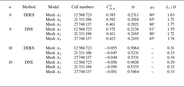
Grid and time-step independence studies were performed. Mesh sensitivity studies were conducted using three progressively refined meshes, denoted as Mesh
 $A_1$
, Mesh
 $A_2$
and Mesh
 $A_3$
. Key flow parameters, including the mean drag coefficient
 $\bar {C}_{D,0}^F$
, Strouhal number
 $St$
, separation angle
 $\varphi _S$
and normalised recirculation length
 $L_r/D$
, were evaluated at rotation rates
 $\alpha =0$
and
 $\alpha =10$
. The recirculation length is defined as the distance between the rear pole of the sphere and the longitudinal position along the axis where the longitudinal velocity changes sign. The results are summarised in tables 2 and 3. The refinement from Mesh
 $A_1$
to Mesh
 $A_2$
leads to a marked improvement in the prediction of both integral and local flow characteristics at
 $\alpha =0$
and
 $\alpha =10$
, as demonstrated by the closer agreement with canonical values of the mean drag coefficient
 $\bar {C}_{D,0}^F$
and the Strouhal number. Further refinement to Mesh
 $A_3$
yields only marginal gains in accuracy while incurring a substantially higher computational cost. Mesh
 $A_2$
is therefore deemed sufficient to resolve the essential unsteady wake dynamics and was selected as an optimal compromise between accuracy and computational efficiency for all subsequent simulations.
Verification of grid independence for flow over a stationary sphere by DNS and DDES.

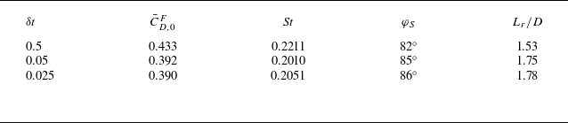
Verification of time-step independence for flow over a stationary sphere by DDES.

Mean non-dimensional velocity and RMS fluctuations at wake centreline points (
 $x/D=2$
, 3, 5, 10 with
 $y=z=0$
) for three mesh resolutions under (a,b) DDES and (a*,b*) DNS frameworks for
 $\alpha =0$
and
 $\alpha =10$
. Error bars indicate fluctuation magnitude.

Simulations were performed using three distinct meshes under both DNS and DDES frameworks to evaluate the mean and RMS values of velocity at four monitoring points for rotation rates of 0 and 10. As illustrated in figure 3(a), for the stationary sphere, DDES results exhibit strong consistency across all meshes, with particularly close agreement between meshes
 $A_2$
and
 $A_3$
in both mean velocity and fluctuations. For the half-rotating sphere at a rotation rate of 10, meshes
 $A_2$
and
 $A_3$
yield closely matching velocity and RMS values, while Mesh
 $A_1$
shows notable deviations (figure 3
b), indicating Mesh
 $A_2$
as the most suitable choice. Corresponding DNS reveal high mesh convergence at zero rotation, with all three meshes producing consistent velocity profiles (figure 3
a*). Similarly, close agreement is observed between meshes
 $A_2$
and
 $A_3$
at a rotation rate of 10 (figure 3
b*). Comparisons between DNS and DDES demonstrate close velocity agreement at zero rotation across all meshes. At a rotation rate of 10, minor discrepancies between DNS and DDES on meshes
 $A_2$
and
 $A_3$
are observed but remain within acceptable limits.
At a time step of
 $\delta t = 0.05$
, the calculated results from the finer meshes
 $A_2$
and
 $A_3$
still exhibit minor discrepancies in the force coefficients; however, these are well within the ranges published in the literature. Consequently, Mesh
 $A_2$
is considered adequate. As shown in table 3, time-step independence was also checked using
 $\delta t = 0.5$
, 0.05 and 0.025 with Mesh
 $A_2$
. Smaller variations were observed between the results of
 $\delta t = 0.05$
and 0.025, indicating that it is appropriate to employ Mesh
 $A_2$
and a time step of
 $\delta t = 0.05$
throughout the study.
The combined mesh and temporal sensitivity analyses validate the numerical approach, showing convergence in key flow quantities. The selection of monitoring points is justified by both literature precedent and their ability to capture significant wake phenomena. The fluctuation quantification methodology via EMD and the RMS value
 $U_{rms}$
facilitate consistent local flow characterisation.
2.2.5. Validation against literature
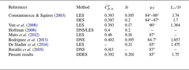
Table 4 presents a comparison of our zero-rotation DDES results with published DNS, LES and DES studies at
 $Re = 1 \times 10^4$
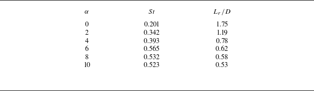
. The present DDES data exhibit excellent consistency with existing DNS and LES findings in both integral and local wake properties. The predicted mean drag coefficient of 0.392 exhibits excellent quantitative agreement with existing DNS, DES and LES results. This close correspondence demonstrates that the present simulations accurately capture the overall hydrodynamic force characteristics of flow past a sphere. The computed Strouhal number of 0.201 aligns well with the canonical vortex-shedding frequency at
 $Re = 1 \times 10^4$
, confirming that the dominant unsteady wake dynamics, including vortex shedding, is well resolved. The separation angle of 85
 $^\circ$
and recirculation length of 1.75 lie within the ranges reported by prior experimental and numerical investigations, indicating that the wake topology and associated length scales are properly captured. Importantly, comprehensive mesh and time-step convergence studies have been conducted to ensure the robustness and reliability of these results. Collectively, these comparisons validate the numerical methodology employed herein and bolster confidence in the accuracy and physical fidelity of the current findings.
Comparison of the mean drag coefficient
 $\bar {C}_{D,0}^F$
, Strouhal number, separation angle
 $\varphi _S$
and recirculation length
 $L_r/D$
for the stationary sphere (
 $\alpha = 0$
) at
 $\delta t=0.05$
on Mesh
 $A_2$
with available literature data at
 $Re = 1 \times 10^4$
.

Considering the substantial computational expense associated with DNS, DDES offers an optimal compromise, balancing accuracy and computational efficiency. Collectively, these results substantiate the selection of Mesh
 $A_2$
coupled with the DDES turbulence model as an appropriate and reliable configuration for the present study.
In summary, comprehensive sensitivity analyses regarding different grid densities and time steps, along with extensive comparisons against existing DNS, LES and DES literature data, have fully validated the reliability and accuracy of the present numerical method. The results demonstrate that the configuration employing Mesh
 $A_2$
coupled with a time step of
 $\delta t = 0.05$
not only accurately captures key flow-field characteristics – including the mean drag coefficient, Strouhal number and wake topological structures – but also achieves an optimal balance between computational accuracy and efficiency within the DDES framework. Furthermore, the high consistency observed between DDES results and high-fidelity DNS results at the extreme rotation rates (
 $\alpha = 0$
and
 $10$
) further confirms the applicability of this hybrid simulation strategy for complex separated flow problems. This validated methodology lays a reliable foundation for the subsequent in-depth exploration of the hydrodynamic characteristics of RBH and RB cases.
3. Results and discussion
This study presents a systematic investigation of flow past a rotating sphere at a subcritical Reynolds number (
 $Re = 1 \times 10^4$
), integrating analyses of force coefficients, force-element terms, vorticity dynamics, surface pressure and power consumption. Utilising FEA, we demonstrate that the half-rotation mode yields simultaneous drag and lift reduction. In terms of drag, a substantial negative velocity drag term effectively counters the rise in volume- and surface-vorticity contributions. Conversely, the net lift is minimised as the attenuation of the surface-vorticity term balances the enhanced volume-vorticity component. The following subsections present this analysis, starting with laminar–turbulent contrasts (§ 3.1) and force coefficient characteristics (§ 3.2). The physical mechanisms governing these forces are elucidated through vorticity-based analysis (§ 3.3), evolution of the vorticity field (§ 3.4) and the mechanism of force cancellation (§ 3.5). Finally, the study examines surface pressure (§ 3.6) and power requirements (§ 3.7), followed by a comprehensive synthesis (§ 3.8).
3.1. Laminar versus turbulent flow
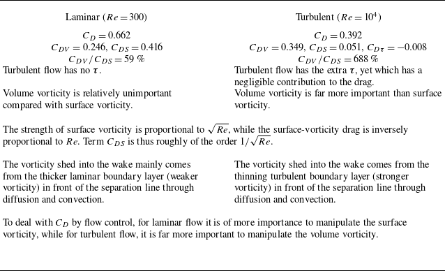
Table 5 summarises the key distinctions between laminar and turbulent flows to contextualise the present investigation. At a low Reynolds number (
 $Re=300$
), the flow past a sphere remains predominantly laminar, with viscous effects dominating and the boundary layer separating early at approximately 67
 $^\circ$
(Seeley, Hummel & Smith Reference Seeley, Hummel and Smith1975) from the front stagnation point. The wake is asymmetric and characterised by a regular hairpin vortex, leading to periodic oscillations in the lift and drag forces. The drag coefficient is relatively high, primarily due to viscous drag, with pressure drag contributing minimally.
Laminar versus turbulent (sphere,
 $\alpha =0$
).

At a higher Reynolds number (
 $Re$
= 10
 $^4$
), the boundary layer transitions to turbulence, delaying separation to approximately 85
 $^\circ$
(Constantinescu & Squires Reference Constantinescu and Squires2003). The wake contracts and exhibits a complex, multi-scale vortical structure, with irregular vortex shedding and high-frequency, low-amplitude force fluctuations. The drag coefficient decreases markedly due to the reduced pressure drag, despite the slightly increased viscous contribution.
Despite these differences, the flows share common features: the upstream pressure distribution remains similar, with a high-pressure region near the stagnation point and a low-pressure region in the wake. In both cases, wake shedding induces unsteady forces, and the fundamental mechanisms of boundary-layer formation, separation and wake generation are consistent across the two Reynolds numbers.
A systematic comparison of the contributions of different force components was conducted from the perspective of FEA, integrating both previous studies and the present results. A detailed summary is provided in table 5.
3.2. Hydrodynamic force validation: statistical characteristics of force coefficients
This section presents the time histories and statistical characteristics of the hydrodynamic force coefficients for a sphere subjected to two drag-reduction strategies: RBH and RB, over a range of rotational speeds
 $\alpha$
from 0 to 10. The primary objective is to validate the effectiveness of these control strategies in drag and lift reduction, providing a quantitative basis for the subsequent fluid dynamic mechanism analysis.
-
(i) For the RBH strategy, as the rotation speed increases from 0 to 10, the mean drag coefficient
$\bar {C}_{D,\alpha }$
decreases monotonically and sharply from 0.392 to
$-0.046$
, while the RMS value of the drag coefficient fluctuations
${A}_{Drms, \alpha }$
remains stable within a small range (approximately 0.0076), as shown in figures 4(a) and 6(a). The mean lift coefficient
$\bar {C}_{L,\alpha }$
and side-force coefficient
$\bar {C}_{S,\alpha }$
both remain close to zero, with RMS fluctuations below 0.02, indicating that this strategy achieves directional drag reduction without introducing significant additional lift or side forces, as shown in figures 4(a), 7 and 8. -
(ii) In contrast, the RB exhibits an initial increase followed by a decrease in the mean drag coefficient
$\bar {C}_{D,\alpha }^F$
, reaching a maximum of 0.605, as shown in figures 4(b) and 6(b–f). The RMS fluctuations increase notably (about 0.07), and both lift and side-force coefficients show substantially higher mean values and fluctuations compared with RBH, reflecting more complex, unsteady flow features and asymmetric force generation, as shown in figures 4(b), 6(b–f), 7 and 8. -
(iii) To facilitate quantitative comparison, five normalised ratios were defined to characterise changes in mean and RMS values of drag, lift and side forces relative to the baseline stationary sphere and the total rotating sphere. Five ratios were defined: the drag reduction ratio
$\eta _1 = {\bar {C}_{D,\alpha }}/{\bar {C}_{D,0}^F}$
, the drag RMS ratio
$\eta _3 = {{A}_{\textit{Drms},\alpha }}/{{A}_{\textit{Drms},0}^F}$
, the lift RMS ratio
$\eta _4 = {{A}_{\textit{Lrms},\alpha }}/{{A}_{\textit{Lrms},0}^F}$
and the side-force RMS ratio
$\eta _5 = {{A}_{\textit{Srms},\alpha }}/{{A}_{\textit{Srms},0}^F}$
associated with the RBH, and the mean lift ratio
$\eta _2 = {\bar {C}_{L,\alpha }}/{\bar {C}_{L,\alpha }^F}$
associated with the RB and RBH. As shown in figure 5, the normalised ratios reveal two distinct force–response regimes: a low-fluctuation, symmetry-preserving regime associated with RBH, and a highly unsteady, asymmetry-dominated regime associated with RB. In particular, under RBH the RMS ratios remain close to unity despite increasing rotation speed, confirming that drag reduction is achieved primarily through modification of the mean momentum balance rather than through enhanced force oscillations.


Drag, lift and side-force coefficients of the sphere for (a) RBH and (b) RB at various rotation speeds
 $\alpha$
.

(a) The drag reduction ratio
 $\eta _1$
and the mean lift ratio
 $\eta _2$
and (b) the drag RMS ratio
 $\eta _3$
, the lift RMS ratio
 $\eta _4$
and the side-force RMS ratio
 $\eta _5$
at various rotation speeds
 $\alpha$
.

Time history of the sphere drag coefficient for RBH (upper) and RB (lower) over
 $0\leqslant t \leqslant 210$
at various rotation speeds
 $\alpha$
.

Time history of the sphere lift coefficient for RBH (a,b) and RB (a*,b*) over
 $0\leqslant t \leqslant 210$
at various rotation speeds
 $\alpha$
.

Time history of the sphere side-force coefficient for RBH (a,b) and RB (a*,b*) over
 $0\leqslant t \leqslant 210$
at various rotation speeds
 $\alpha$
.

In summary, the two rotational strategies, RBH and RB, exhibit fundamentally different force–response characteristics. Under the RBH configuration, a substantial reduction in drag is accompanied by low-amplitude force fluctuations, while both lift and side-force components remain close to zero. This behaviour indicates that RBH achieves drag reduction while preserving force stability and directional symmetry. In contrast, the RB configuration is characterised by markedly stronger unsteady fluctuations across all force components, together with pronounced transverse force responses, reflecting a more unstable and dynamically complex force behaviour. It should be emphasised that the above observations are based solely on force time histories and their statistical properties, and therefore are insufficient to establish a direct causal link between the observed force modulation and the underlying flow structures.
Therefore, a more detailed flow-field analysis is required to elucidate the physical mechanisms underlying the distinct force responses induced by different rotational strategies. Accordingly, § 3.3 systematically investigates the characteristic flow structures under RBH and RB conditions, focusing on the spatial distribution of vorticity in the windward boundary layer and the shear layer–recirculation region interface, variations in the spatial scale of the recirculation zone, as well as the distributions of surface pressure and separation lines. The objective of this analysis is to reveal the fluid-dynamical mechanisms by which half-rotation achieves effective drag reduction while simultaneously suppressing transverse forces and force fluctuations.
3.3. Vorticity-based force analysis and flow physics
Vorticity plays a central role in governing the dynamics of separated bluff-body flows and the associated hydrodynamic force generation. In such flows, the production, redistribution and transport of vorticity determine momentum exchange, wake topology and pressure imbalance, and thereby directly control drag, lift and side-force characteristics. Motivated by this fundamental connection, the present section analyses the flow physics and force-generation mechanisms from a vorticity-based perspective, with particular emphasis on how near-wall vorticity generation, shear-layer separation and wake transport contribute to the net hydrodynamic forces under different drag-reduction strategies.
To establish a direct and physically interpretable link between local flow structures and global force responses, FEA is employed. This framework decomposes the total hydrodynamic forces into contributions associated with surface vorticity, volume vorticity, velocity-related terms and Reynolds stresses, thereby enabling a quantitative assessment of the relative importance of different vorticity-related mechanisms. Central to this formulation is the volume-vorticity force, which involves the Lamb vector
 $\boldsymbol{u}\times \boldsymbol{\omega }$
and its projection onto an auxiliary potential velocity field. This term provides a natural bridge between classical vorticity-flux concepts and the force contributions arising from boundary-layer generation, shear-layer separation and downstream vortex shedding.
In what follows, the force coefficients are first decomposed using FEA to identify the dominant contributing terms. Attention is then focused on the spatial distribution and restructuring of volume-vorticity force elements in key regions of the flow, including the upstream boundary layer, the separated shear layer and the shear layer–recirculation interface. Through this analysis, the physical mechanisms by which vorticity transport and alignment are modified under different control strategies are elucidated, together with their implications for drag reduction and lift reduction.
(A) Vorticity-based framework and force-element formulation
Vorticity is a fundamental quantity characterising local fluid rotation and plays a central role in shaping the dynamical structure of separated flows. In bluff-body hydrodynamics, the redistribution of vorticity governs momentum transport, wake topology and pressure imbalance, thereby directly influencing hydrodynamic forces. The vorticity magnitude distributions shown in figure 9 confirm that the upstream boundary layer, the separated shear layer and the interface between the shear layer and the recirculation zone are regions of high intensity in both the velocity and vorticity fields.
Vorticity contour plot representing vorticity values around the sphere on slices from
 $z = -0.48$
to
 $z = 0.48$
at 0.12 intervals for RBH (a–f) and RB (a*–f*).

Regarding solid boundaries, Lighthill (Reference Lighthill and Rosenhead1963) first defined the boundary vorticity flux for a flat surface, which quantifies the rate of vorticity generation per unit length. Subsequently, Panton (Reference Panton1984) and Lyman (Reference Lyman1990) proposed alternative expressions,
 $\sigma ^{\prime }=-\nu \hat {n}\boldsymbol{\cdot }\boldsymbol{\nabla }\omega$
and
 $\sigma =\nu \hat {n}\times (\boldsymbol{\nabla }\times \omega )$
, respectively. Later studies demonstrated that Lyman’s formulation is more robust under complex boundary conditions (Terrington, Hourigan & Thompson Reference Terrington, Hourigan and Thompson2021). Beyond boundary fluxes, Huggins (Reference Huggins1971, Reference Huggins1994) introduced the vorticity-flux tensor to describe the transport and diffusion of vorticity within the flow field. Anderson (Reference Anderson1966) further established the Josephson–Anderson relation, which directly links hydrodynamic forces to vorticity transport. Using this framework, Du & Zaki (Reference Du and Zaki2025) showed that drag on spheres and spheroids is dominated by wall viscous fluxes and shear-layer advection, with negligible contribution from wake vortices.
Building upon these developments, Chang (Reference Chang1992) introduced FEA, which incorporates auxiliary potential flow to establish a direct and mechanically interpretable link between hydrodynamic forces and both surface and volume vorticity.
Historically, the vector product
 $\boldsymbol{u} \times \boldsymbol{\omega }$
is known as the Lamb vector (Lamb Reference Lamb1932), which is non-zero whenever the velocity
 $\boldsymbol{u}$
and vorticity
 $\boldsymbol{\omega }$
are not parallel. In particular, within two-dimensional boundary layers,
 $\boldsymbol{u}$
and
 $\boldsymbol{\omega }$
are approximately orthogonal, rendering the Lamb vector a fundamental component of the volume-vorticity force contribution.
The volume-vorticity force element
 $\boldsymbol{u} \times \boldsymbol{\omega } \boldsymbol{\cdot }\boldsymbol{\nabla }\phi _i$
indicates that the force contribution is governed by the degree of alignment between the Lamb vector and the auxiliary potential velocity
 $\boldsymbol{\nabla }\phi _i$
. Depending on the relative orientation of the triad
 $(\boldsymbol{u}, \boldsymbol{\omega }, \boldsymbol{\nabla }\phi _i)$
, this contribution may be positive or negative. Here,
 $\boldsymbol{\nabla }\phi _i$
, defined in (2.9), represents the auxiliary potential velocity field. Physically, the scalar product
 $\boldsymbol{u} \times \boldsymbol{\omega } \boldsymbol{\cdot }\boldsymbol{\nabla }\phi _i$
measures the extent to which the Lamb vector is transported along the potential velocity; if the Lamb vector is perpendicular to
 $\boldsymbol{\nabla }\phi _i$
, the corresponding volume-vorticity force element vanishes.
This interpretation naturally admits a flux-based viewpoint. The Lamb vector
 $\boldsymbol{u} \times \boldsymbol{\omega }$
may be regarded as a local transport flux associated with vorticity-related momentum. When projected onto the auxiliary potential velocity
 $\boldsymbol{\nabla }\phi _i$
, the volume-vorticity force element effectively measures the component of this flux that crosses the potential field associated with
 $\phi _i$
. Within this framework, the volume-vorticity force is fully consistent with the Josephson–Anderson and Huggins formulations of vorticity flux, providing a unified description that links near-wall vorticity generation, boundary-layer separation and downstream vortex shedding to the resulting hydrodynamic force contributions.
(B) Force decomposition and dominant contributions
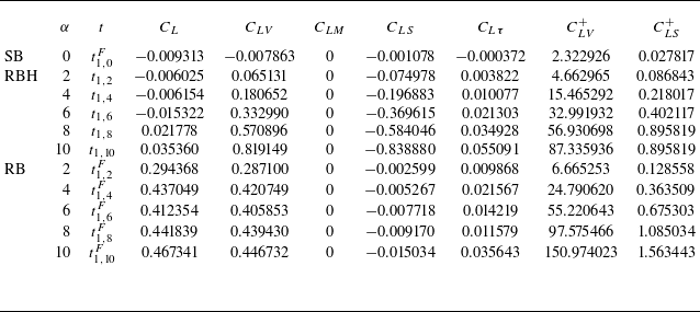
The FEA provides a diagnostic tool for relating local flow structures to the hydrodynamic forces on bluff bodies. In this study, the force coefficients are decomposed into volume-vorticity force, surface-vorticity force, velocity force and Reynolds stress contributions. The results show that the force coefficients are primarily governed by the volume-vorticity force term, velocity force term and surface-vorticity force term, whereas the Reynolds stress contribution is negligible (see tables 6–8). Notably, under the RBH strategy, the velocity force contribution to drag is negative, while its contributions to lift and side force vanish. In contrast, under the RB strategy, the velocity force contributions to drag, lift and side force are all zero.
Instantaneous volume- and surface-vorticity drag terms in (2.16) for the baseline SB and the controlled cases (RBH, RB) at
 $Re = 1 \times 10^4$
, evaluated at selected times (
 $t_{1, 2}{-}t_{1, 10}$
and
 $t_{1, 0}^F{-}t_{1, 10}^F$
) corresponding to figure 6. Absolute values of the volume terms in (3.2) and surface terms in (3.5).

Instantaneous volume- and surface-vorticity lift terms in (2.21) for the baseline SB and the controlled cases (RBH, RB) at
 $Re = 1 \times 10^4$
, evaluated at selected times (
 $t_{1, 2}{-}t_{1, 10}$
and
 $t_{1, 0}^F{-}t_{1, 10}^F$
) corresponding to figure 6. Absolute values of the volume terms in (3.3) and surface terms in (3.6).

Instantaneous volume- and surface-vorticity side-force terms in (2.27) for the baseline SB and the controlled cases (RBH, RB) at
 $Re = 1 \times 10^4$
, evaluated at selected times (
 $t_{1, 2}{-}t_{1, 10}$
and
 $t_{1, 0}^F{-}t_{1, 10}^F$
) corresponding to figure 6. Absolute values of the volume terms in (3.4) and surface terms in (3.7).

The volume-vorticity force primarily originates from regions of intense vorticity, including the upstream boundary layer, the separated shear layer and the shear layer–recirculation interface, whereas the surface-vorticity force reflects the contribution of vorticity on the sphere surface. The velocity force term arises solely from body motion and is identically zero for a stationary sphere.
(C) Spatial distribution of volume-vorticity force elements
To further quantify the spatial organisation of the volume-vorticity force, nine cross-sectional planes normal to the
 $z$
direction were extracted uniformly at intervals of 0.12 within the range
 $-0.48 \le z \le 0.48$
. The contour maps on these planes display the magnitude and sign of the volume-vorticity drag, lift and side-force elements, given respectively by
 $-( {8}/{\pi })\boldsymbol{u}\times \boldsymbol{\omega }\boldsymbol{\cdot }\boldsymbol{\nabla }\phi _i$
(2.16),
 $-( {8}/{\pi })\boldsymbol{u}\times \boldsymbol{\omega }\boldsymbol{\cdot }\boldsymbol{\nabla }\phi _j$
(2.21) and
 $-( {8}/{\pi })\boldsymbol{u}\times \boldsymbol{\omega }\boldsymbol{\cdot }\boldsymbol{\nabla }\phi _k$
(2.26). The corresponding spatial distributions are presented in figures 12–14, respectively.
For the RBH case, the vortex structures remain highly organised. In the drag direction, positive and negative volume-vorticity elements remain distinctly separated (figure 12 a–f); although their contribution to drag is large, it is substantially offset by the velocity drag term, thereby achieving drag reduction. In the lift direction, the positive and negative elements also remain orderly and distinct (figure 13 a–f). While the volume-vorticity lift term gradually increases, it is partially counteracted by the decrease in the surface-vorticity lift term, thus maintaining a relatively small net lift. In contrast, for the RB case, the fragmented vortices cause the positive and negative volume-vorticity elements in the drag direction to largely cancel each other, resulting in a pronounced reduction in the volume-vorticity drag term (figure 12 a*–f*). In the lift direction, although positive and negative elements also cancel, the Magnus effect progressively increases the volume-vorticity lift term (figure 13 a*–f*).
Based on the above analysis, the subsequent discussion focuses on how vorticity distribution and the associated volume-vorticity force elements are restructured in these key regions under different drag-reduction strategies.
3.3.1. Baseline flow structure and force generation for a stationary sphere
In turbulent flow around a stationary sphere at a Reynolds number of 10
 $^4$
, the incoming flow forms a stable, symmetric laminar boundary layer over the upstream surface of the stationary sphere. Due to the strong adverse pressure gradient along the longitudinal direction, the boundary layer separates near the shoulder of the sphere. Downstream of separation, a well-defined separated shear layer develops between the high-speed outer flow and the low-momentum recirculation region, as clearly identified by the vorticity magnitude distribution shown in figure 9(a).
The no-slip condition at the sphere surface generates steep velocity gradients within the boundary layer, producing significant vorticity that directly influences separation and force generation. At the interface between the separated shear layer and the recirculation zone, the longitudinal velocity decays rapidly towards the wake centre, giving rise to intense velocity gradients and, consequently, concentrated vorticity. These regions constitute the dominant source of the volume-vorticity force acting on the sphere.
An examination of the
 $ z$
-vorticity distribution within the upstream boundary layer reveals a systematic sign change across the midplane: negative
 $ z$
vorticity in the region
 $ x\lt 0, y\gt 0$
and positive
 $ z$
vorticity in
 $ x\lt 0, y\lt 0$
(figures 10
a and 11
a). This distribution reflects the opposite directions of velocity shear in the upper and lower halves of the boundary layer and provides a symmetric reference state for assessing symmetry breaking under RBH and RB.
Distributions of
 $z$
vorticity on the symmetry plane (
 $z = 0$
) for RBH (a–f) and RB (a*–f*) at indicated rotation rates.

Distributions of
 $z$
vorticity around the sphere on slices from
 $x = 0$
to
 $z = 1.5$
at 0.3 intervals for RBH (a–f) and RB (a*–f*).

The FEA results show that, for the stationary sphere, both drag and lift are governed by the volume-vorticity force term and the surface-vorticity force term, while the Reynolds-stress contribution is negligible and the velocity force term is identically zero. Quantitatively, the volume-vorticity drag term
 $C_{DV}$
is approximately seven times greater than the corresponding surface-vorticity drag term
 $C_{DS}$
(0.35 versus 0.05), the volume-vorticity lift term
 $C_{LV}$
is about eight times larger than the surface-vorticity lift term
 $C_{LS}$
(−0.008 versus −0.001) and, similarly, the volume-vorticity side-force term
 $C_{SV}$
is about fourteen times larger than the surface-vorticity side-force term
 $C_{SS}$
(−0.014 versus −0.001), as shown in tables 6–8. This indicates that all the drag, lift and side force are predominantly governed by the volume-vorticity force term, where the contributing vorticity originates primarily from the boundary layer on the windward side and the interaction region between the shear layer and the recirculation zone.
-
(i) As shown in figure 12(a), the volume-vorticity drag elements
$-( {8}/{\pi })\boldsymbol{u}\times \boldsymbol{\omega } \boldsymbol{\cdot }\boldsymbol{\nabla }\phi _{i}$
at the front side of the sphere that provide a negative contribution to the drag (indicated in blue) mainly originate from the upstream boundary layer. In contrast, the strong positive contribution of the volume-vorticity drag elements at the back side of the sphere to drag (indicated in red) is mainly concentrated in the shear layer–circulation return flow interface region, which is the main source of drag. The velocity gradient within the recirculation zone is relatively weak, and the volume-vorticity drag elements in this region contribute less to the drag. -
(ii) For lift and side force, the boundary layer on the windward surface and the interface between the shear layer and the recirculation zone remain the primary source regions for the volume-vorticity force elements, which is consistent with the spatial distribution of the drag generation mechanism. (a) For lift, the vorticity in the regions of
$ y \gt 0$
and
$ y \lt 0$
contributes oppositely but comparably in magnitude to the volume-vorticity lift element
$-( {8}/{\pi })\boldsymbol{u}\times \boldsymbol{\omega } \boldsymbol{\cdot }\boldsymbol{\nabla }\phi _{j}$
, as shown in figure 13(a). In the upper region (
$ y \gt 0$
), the vorticity corresponds to a positive contribution (region with red colour) to the volume-vorticity lift element, while in the lower region (
$ y \lt 0$
), the vorticity corresponds to a negative contribution (region with blue colour). It is this antisymmetric distribution about the plane
$ y = 0$
that causes the integral of the lift volume-vorticity force elements in the lift direction to nearly cancel out, resulting in the lift being close to zero. (b) Similarly, for the side force, the volume-vorticity side-force elements
$-( {8}/{\pi })\boldsymbol{u}\times \boldsymbol{\omega } \boldsymbol{\cdot }\boldsymbol{\nabla }\phi _{k}$
exhibit an antisymmetric distribution about the plane
$ z = 0$
, as shown in figure 14(a). In the region
$ z \gt 0$
, the vorticity contributes positively (region with red colour) to the volume-vorticity side force, while in the region
$ z \lt 0$
, it contributes negatively (region with blue colour). This antisymmetric distribution about the plane
$ z = 0$
causes the integral of the volume-vorticity side-force element in the side-force direction to nearly cancel out, resulting in the side force being close to zero. This cancellation reflects the overall axisymmetry of the velocity, vorticity and separation structures for the stationary sphere.


Thus, the generation of drag, lift and side force all stems from the spatial distribution of the vorticity structure in the windward boundary layer, shear layer and the interface with the recirculation zone.
Comparison of the volume-vorticity drag element
 $-({8}/{\pi })\boldsymbol{u}\times \boldsymbol{\omega }\boldsymbol{\cdot }\boldsymbol{\nabla }\phi _{i}$
between RBH (a–f) and RB (a*–f*) at various rotation rates.

Comparison of the volume-vorticity drag element
 $-({8}/{\pi })\boldsymbol{u}\times \boldsymbol{\omega }\boldsymbol{\cdot }\boldsymbol{\nabla }\phi _{j}$
between RBH (a–f) and RB (a*–f*) at various rotation rates.

Comparison of the volume-vorticity drag element
 $-({8}/{\pi })\boldsymbol{u}\times \boldsymbol{\omega }\boldsymbol{\cdot }\boldsymbol{\nabla }\phi _{k}$
between RBH (a–f) and RB (a*–f*) at various rotation rates.

3.3.2. Flow reorganisation
In the RBH configuration, where the sphere rotates about the negative
 $z$
axis, tangential momentum is energised and injected directly into the boundary layer. This rotational forcing first modifies the near-wall flow and subsequently propagates downstream through separation into the shear layer and wake. At the shear-layer–recirculation interface, longitudinal velocity decreases rapidly both towards the wake centre and towards the free stream, producing strong velocity gradients that intensify vorticity generation. These high-vorticity regions play a decisive role in determining both drag and lift.
Figures 10 and 11 illustrate the variation of the spanwise vorticity
 $\omega _z$
with rotation rate
 $\alpha$
for the RBH and RB cases. At
 $\alpha =0$
, negative (blue) vorticity dominates the upper shear layer, while the lower side exhibits positive (red) vorticity (figures 10
a and 11
a). In the RBH case, increasing
 $\alpha$
progressively reorganises the vorticity field: positive vorticity first appears in the upper-left region at
 $\alpha =2$
(figures 10
b and 11
b); at
 $\alpha =4$
, positive structures emerge in both the lower- and upper-left regions (figures 10
c and 11
c); at
 $\alpha =6$
, the upper positive vorticity region expands (figures 10
d and 11
d); and for
 $\alpha \geq 8$
, the negative vorticity in the wake becomes fully enclosed by two positive regions (figures 10
e and 11
e). This progression reveals a systematic modification of the wake topology by the RBH strategy.
By contrast, in the RB case, the
 $z$
-component vorticity on the
 $z=0$
plane exhibits a more irregular and fragmented distribution, as shown in figures 10(a*–f*) and 11(a*–f*), indicating less coherent rotational structures. This comparison underscores the enhanced capability of the RBH strategy to control wake vorticity and reorganise the flow topology, highlighting its superior effectiveness for drag reduction.
(A) Boundary-layer and vorticity restructuring on the windward hemisphere
Localised upstream rotation entrains near-wall fluid and superposes rotational motion onto the incoming flow, forming an asymmetric high-speed rotating boundary-layer band. Owing to the relative orientation between the imposed rotation and the free stream, the near-wall flow exhibits a pronounced asymmetry: in the region
 $ y\lt 0$
, the free stream weakens the rotational motion, whereas in
 $ y\gt 0$
, the rotation and free stream act cooperatively, significantly accelerating the boundary layer, as shown in figure 9(b–f). As a result, the thickness of the rotation-dominated near-wall region is minimal near
 $ y=-0.5D$
and increases progressively towards
 $ y=0.5D$
, with the overall thickness growing monotonically with rotation rate. This asymmetric acceleration leads to a systematic reorganisation of the boundary-layer vorticity field, as is shown in figures 10(b–f) and 11(b–f). Specifically, in the region
 $ y\gt 0$
, the
 $ z$
vorticity reverses sign from negative in the stationary case to positive under rotation, while in
 $ y\lt 0$
, it remains positive. This restructuring of vorticity provides the dynamical foundation for the subsequent reconstruction of the volume-vorticity force elements.
These topological variations translate directly into modifications of the volume-vorticity force elements. Under the RBH strategy, increasing the rotation rate induces a systematic evolution of these volume force contributions.
-
(i) In the drag direction, portions of the upstream boundary layer that previously contributed negatively (highlighted in blue) to the volume-vorticity drag element
$-( {8}/{\pi })\boldsymbol{u}\times \boldsymbol{\omega } \boldsymbol{\cdot }\boldsymbol{\nabla }\phi _{i}$
now generate positive contributions (indicated in red), particularly in (
$x\lt 0, y\gt 0$
). Meanwhile, in the region (
$x\lt 0, y\lt 0$
), at a certain distance from the wall, they still provide a negative contribution to the volume-vorticity drag element (figure 12
a–f). -
(ii) In the lift direction, the distribution of the volume-vorticity lift element
$-( {8}/{\pi })\boldsymbol{u}\times \boldsymbol{\omega } \boldsymbol{\cdot }\boldsymbol{\nabla }\phi _{j}$
becomes strongly asymmetric. Specifically, in the region (
$x\lt 0, y\gt 0$
), the volume-vorticity lift elements for lift switch from positive to negative compared with the stationary case. Additionally, near the sphere surface within the (
$x\lt 0, y\lt 0$
) region, the positive volume-vorticity lift elements for lift appear, while further away, the negative volume-vorticity lift elements continue to dominate (figure 13
a–f). -
(iii) In the side-force direction, the left half of the sphere changes from negative to positive volume-vorticity side-force element
$-( {8}/{\pi })\boldsymbol{u}\times \boldsymbol{\omega } \boldsymbol{\cdot }\boldsymbol{\nabla }\phi _{k}$
, while the right half changes from positive to negative. At a rotation speed of 10, negative elements (blue) are mainly found in the (
$x\lt 0, y\gt 0, z\gt 0$
) and (
$x\lt 0, y\lt 0, z\lt 0$
) regions, while positive elements (red) are located in the (
$x\lt 0, y\lt 0, z\gt 0$
) and (
$x\lt 0, y\gt 0, z\lt 0$
) regions (figure 14
a–f).


(B) Shear-layer–recirculation interaction and vorticity restructuring
Downstream of separation, localised upstream rotation continuously supplies momentum to the separated shear layer, maintaining elevated velocity levels, especially on the sphere-facing side of the shear layer. From the shear-layer–recirculation interface, velocity decays rapidly both towards the wake core and towards the free stream, generating intense velocity gradients. A strong velocity gradient corresponds directly to an intensified vorticity magnitude. Due to the upstream hemisphere of the sphere rotating about the negative
 $ z$
axis, the momentum primarily influences the shear-layer region where
 $ x \gt 0$
and
 $ y \gt 0$
, which is the focus area of this study. In this region, the recirculation zone is significantly suppressed. Unlike the negative
 $ z$
vorticity directed towards the recirculation zone, positive
 $ z$
vorticity appears at the shear-layer–recirculation interface pointing towards the free stream. This contrast between positive and negative vorticity forms a distinct boundary at the interface, as shown in figures 10 and 11.
-
(i) At the shear-layer–recirculation interface directed towards the recirculation zone, the
$ z$
vorticity remains consistent with that of the stationary sphere: negative in the region
$ y \gt 0$
and positive in
$ y \lt 0$
(see figure 10
b–f). The signs of the volume-vorticity force elements contributing to drag, lift and side force similarly remain consistent with the stationary case, as depicted in figures 12–14. Despite the unchanged signs, the intensities of these vorticities and force elements increase. -
(ii) In the region of the interface pointing towards the free stream (
$ x \gt 0, y \gt 0$
), strong positive
$ z$
vorticity arises due to the large velocity gradient (indicated in red in figure 10
b–f). Within this region, the
$ z$
vorticity is positive (red), the volume-vorticity drag elements
$-( {8}/{\pi })\boldsymbol{u}\times \boldsymbol{\omega } \boldsymbol{\cdot }\boldsymbol{\nabla }\phi _{i}$
for drag are negative (blue), the volume-vorticity lift elements
$-( {8}/{\pi })\boldsymbol{u}\times \boldsymbol{\omega } \boldsymbol{\cdot }\boldsymbol{\nabla }\phi _{j}$
for lift are negative (blue), while the volume-vorticity side-force elements
$-( {8}/{\pi })\boldsymbol{u}\times \boldsymbol{\omega } \boldsymbol{\cdot }\boldsymbol{\nabla }\phi _{k}$
for side force are negative in the
$ z \gt 0$
region (blue) and positive in the
$ z \lt 0$
region (red), as depicted in figures 12–14. As the rotation rate increases, the spatial extent and intensity of the
$ z$
-vorticity and volume-vorticity force elements for drag, lift and side force gradually grow.


The stark contrast in flow topology between RB and RBH stems from the fundamental difference in momentum injection mechanisms. In the RB case, the rotation of the entire surface induces a global boundary condition that extends to the leeward side. Although the windward rotation energises the boundary layer, the simultaneous rotation of the leeward surface creates continuous fluid entrainment and strong shear at the wake boundary. This competing mechanism prevents the shear layers from closing symmetrically, resulting in a highly unstable flow field. As the rotation rate increases (e.g. at
 $\alpha =10$
), the spatial arrangement becomes extremely disordered and fragmented (figure 12–14, right-hand panels). In sharp contrast, RBH injects momentum exclusively to counteract the adverse pressure gradient on the upstream side, allowing the downstream wake to close naturally. This targeted control suppresses randomness and fosters a highly organised shear layer, ultimately resulting in a significantly narrower and more stable wake structure.
This topological difference dictates the hydrodynamic forces through the alignment of force elements. Indeed, the contribution of the volume-vorticity force is physically governed by the degree of alignment between the Lamb vector
 $\boldsymbol{u}\times \boldsymbol{\omega }$
and the auxiliary potential velocity
 $\boldsymbol{\nabla }\phi _i$
(Anderson Reference Anderson1966; Huggins Reference Huggins1971, Reference Huggins1994). For the RB case, the fragmented shear layer leads to poor spatial coherence, causing positive and negative force elements to coexist and undergo significant mutual cancellation. This theoretical basis explains the apparent contradiction in force magnitudes: although RB exhibits stronger overall vorticity activity (figure 19), the lack of structural coherence results in a surprisingly small net volume-vorticity drag
 $C_{DV}$
.
Conversely, the RBH configuration maintains a highly coherent vorticity structure due to its narrower and organised shear layer. This organisation ensures an effective and persistent alignment between the Lamb vector and the potential field, yielding a substantially larger net
 $C_{DV}$
. However, this large volume drag is effectively counteracted by the dominant negative velocity drag term induced by the front-hemisphere rotation, resulting in significant total drag reduction. For lift, RBH effectively balances volume- and surface-vorticity terms to suppress the net lift, whereas RB is dominated by the Magnus effect. These findings elucidate the fundamentally different physical processes: RB relies on cancellation via fragmentation, while RBH relies on organised structure and inter-element compensation.
3.3.3. Drag reduction dominated by the velocity drag term
Comparison of the force-element terms between RBH (a–c) and RB (a*–c*) across various rotation rates.

In the preceding analysis, the distribution of the volume-vorticity force elements in the upstream boundary layer and near the shear-layer–recirculation interface has been examined in detail. Building on these observations, we now perform a volumetric integration of the volume-vorticity drag elements to quantitatively evaluate the magnitude of the volume-vorticity force in the drag direction. Quantitatively, increasing the rotation rate from 0 to 10 leads to systematic changes in the volume-vorticity force, surface-vorticity force and velocity force contributions to drag, lift and side force, as summarised below.
-
(i) In the drag direction, the volume-vorticity force rises sharply from 0.35 to 74.49, while the surface-vorticity force increases modestly from 0.05 to 0.45, as shown in table 6 and figure 15(a). In contrast, the velocity drag term decreases from zero to approximately
$-75$
, effectively counterbalancing the combined positive contributions of the vorticity forces and resulting in a net drag reduction. Despite the substantial increase in positive volume-vorticity force under localised upstream rotation, drag reduction is ultimately achieved through the emergence of a large negative velocity drag term. -
(ii) In the lift direction, the velocity lift term is zero. Here, the increase in volume-vorticity force (from
$-0.008$
to 0.819) is offset by a comparable decrease in surface-vorticity force (from
$-0.001$
to
$-0.839$
), maintaining near-zero lift across the examined rotation rates, as shown in table 7 and figure 15(b). -
(iii) In the side-force direction, the velocity side-force term is zero. Here, both the volume-vorticity force and the surface-vorticity force are very small, maintaining near-zero side force across the examined rotation rates, as shown in table 8 and figure 15(c).


Under both RBH and RB cases, rotation increases the surface-vorticity term contributing to drag, whereas the surface-vorticity term associated with lift decreases and contributes negatively. Quantitatively, in the RBH case, the volume-vorticity drag term
 $C_{DV}$
dominates, being roughly 165 times larger than the surface-vorticity drag term
 $C_{DS}$
(74.49 versus 0.45). In stark contrast, under RB conditions, the volume and surface drag terms are of comparable magnitude (0.21 versus 0.19), as detailed in table 6. Although rotation enhances
 $C_{DS}$
in both cases, the amplification is approximately twice as large in RBH compared with RB.
Regarding lift, the RBH configuration exhibits a distinct cancellation mechanism: the positive contribution from the volume-vorticity term is nearly neutralised by a negative contribution of equal magnitude from the surface-vorticity term, yielding a ratio close to −1 (0.82 versus −0.84). Conversely, in the RB case, the surface-vorticity term is negligible, leaving the volume-vorticity term (0.45) to dominate the lift generation (see table 7). Notably, while rotation reduces the surface-vorticity contribution to lift in both cases, this reduction is significantly more pronounced in the RBH case.
In conclusion, although the RBH strategy induces a substantial increase in the volume-vorticity drag term
 $C_{DV}$
, this effect is effectively counterbalanced by the pronounced negative contribution of the velocity drag term
 $C_{\textit{DM}}$
, thereby significantly attenuating the total drag. This dynamic interplay stems from the flow reorganisation induced by the half-sphere rotation: the stabilisation of the upstream boundary layer delays separation, while the wake vorticity redistribution modifies the global pressure field. A parallel compensatory mechanism governs the lift: although RBH generates a large volume-vorticity lift term
 $C_{LV}$
due to asymmetric vortex shedding, the surface-vorticity lift term
 $C_{LS}$
acts as a counterbalance to suppress the net lift force. These findings underscore the essential role of inter-element coupling: effective flow control does not merely rely on reducing individual force components, but rather on orchestrating a strategic balance between volume- and surface-based contributions to reshape the global hydrodynamic force signature.
3.3.4. Unified interpretation: wake suppression and delayed separation
The RBH configuration alters the momentum balance in the boundary layer and wake. Enhanced near-wall momentum transport delays separation, shifts the separation line downstream and compresses the recirculation region. The normalised recirculation length
 $ L_r/D$
decreases monotonically from approximately 1.75 in the stationary case to about 0.3 at high rotation rates, indicating a substantial contraction of the low-pressure wake region, as shown in table 9 and figure 16.
Variation of the Strouhal number and normalised recirculation length with the rotation rate
 $\alpha$
for flow past a sphere under RBH at Reynolds number (
 $Re = 1 \times 10^4$
).

The
 $x$
-direction velocity distribution of the sphere wake region for RBH (a–f) and RB (a*–f*) at various rotation speeds.

Surface friction lines on the sphere at (a)
 $\alpha =0$
and (b)
 $\alpha =8$
(RBH). The left- and right-hand columns represent the viewpoints along the negative
 $z$
axis and negative
 $x$
axis, respectively.

Although vorticity intensifies locally near the shear-layer–recirculation interface, drag reduction does not arise from a weakening of vorticity forces but from a global reorganisation of the flow that introduces a dominant negative velocity drag term. The combined effects of delayed separation and wake suppression therefore constitute the primary physical mechanism underlying drag reduction in the present configuration.
To investigate the flow patterns near the wall, we present plots of the surface friction lines, which are defined by the following streamline equation:
 \begin{equation} \begin{aligned} \frac {{\rm d}x}{\tau _{wx}} = \frac {{\rm d}y}{\tau _{wy}}=\frac {{\rm d}z}{\tau _{wz}}, \end{aligned} \end{equation}
where
 $(\tau _{wx}, \tau _{wy}, \tau _{wz})$
is the surface stress vector. These patterns are analysed for both the stationary sphere (SB) and the selected case of half-rotation (RBH) with
 $\alpha = 8$
. Figure 17(a,b) displays two perspective views of the surface friction lines: the side view on the
 $z=0$
plane and the rear view on the
 $x=0$
plane.
-
(i) Stationary sphere (SB,
$\alpha = 0$
). The surface line of primary separation (LS) is approximately axisymmetric, occurring at
$\theta \approx 95^\circ$
(relative to the rear stagnation point (RSP) located at
$(R, 0, 0)$
, or
$85^\circ$
from the front stagnation point (FSP) located at
$(-R, 0, 0)$
), which is consistent with reported laminar separation data (Constantinescu & Squires Reference Constantinescu and Squires2003). The separation behaviour is nearly normal; that is, the surface friction lines on both sides of the LS converge normally towards the separation line. The FSP serves as the origin from which surface friction lines emanate and extend downstream. Conversely, the surface friction lines on the rear side of the sphere exhibit a complicated pattern in that: (a) on the left-hand side, moving from the upper to the lower regions, one can observe in sequence a local line of reattachment, a local line of secondary separation, another local line of secondary reattachment and a final line of a third separation and (b) on the right-hand side, there exists an origin from which the surface friction lines emanate radially towards all identified separation lines: the primary separation line, the secondary separation line and the third separation line. -
(ii) Half-rotating sphere (RBH,
$\alpha = 8$
). The surface friction lines exhibit a significantly more complex pattern characterised by a high level of distortion. (a) Side view: We first identify the dividing line (DL), the LS and the line of stagnation (LG). The DL is generated primarily due to the half-rotation effect. Consequently, on the two sides of the upper DL, the surface friction lines move in opposite directions; however, on the two sides of the lower DL, the surface friction lines run in the same direction. This reversed trend occurs near the middle of the DL, in the vicinity of which we observe the division of the LS and the LG. Detailed discussions of the LS and LG are provided in the rear-view analysis. (b) Rear view: On the upper surface, it is observed that the LS is disconnected between the central shoulder region and the lateral regions. In the central shoulder area, the downstream rotation of the front half is so strong that the separation point at each azimuth angle
$\phi$
is pushed further downstream along the surface, forming a cusp-like curve. On the lateral sides, where the downstream rotation is weaker, the separation point retreats backward and increases slowly as the distance from the shoulder region increases. The separation behaviour is no longer normal, as the friction lines on both sides of the LS converge obliquely towards the separation line. On the lower surface, the upstream rotation of the front half leads to a clearly identified LG, occurring uniformly at
$\theta \approx -75^\circ$
. The stagnation behaviour is also not normal, with friction lines on both sides of the LG obliquely converging towards the stagnation line. Meanwhile, the surface friction lines in the region between the LS and LG exhibit a versatile pattern where phenomena similar to those of the SB case, such as alternating reattachment and secondary separation, can be observed. -
(iii) In the RBH configuration, the separation topology becomes strongly three-dimensional. On the upper sphere (
$y\gt 0$
), the rotation-induced near-wall motion injects tangential momentum that strengthens the boundary layer against the adverse pressure gradient. Consequently, the separation line migrates progressively downstream towards the RSP. As
$\alpha$
increases from 0 to 10, the separation angle
$\theta _S$
(measured from the RSP at
$(R, 0, 0)$
) decreases markedly from
$95^\circ$
to
$14^\circ$
, reflecting a significant shift towards the rear pole. At sufficiently high rotation rates (
$\alpha = 8$
–
$10$
), the separation line exhibits a pronounced arrow-like deformation. This downstream shift significantly recovers surface pressure on the rear hemisphere, decreasing total drag. In contrast, on the lower sphere (
$y\lt 0$
), the rotation-driven near-wall flow opposes the free stream. The outer flow does not attach to the windward surface but instead bypasses the sphere, forming a shear layer between the downstream-moving free stream and the rotation-driven near-wall flow. The upstream termination of this shear layer defines a stagnation point, and the connected locus forms a stagnation line. As the rotation rate increases from
$\alpha = 2$
to
$10$
, the position of the stagnation line on the lower hemisphere remains almost unchanged.


Overall, the RBH configuration induces a global reorganisation of the flow field through asymmetric separation control. The rotation-induced momentum injection on the upper surface effectively suppresses the adverse pressure gradient, causing the separation point to migrate downstream to
 $\theta _S \approx 14^\circ$
. Conversely, the lower surface features a flow-opposing mechanism that anchors a stagnation line at a nearly constant position (
 $\theta _G \approx -75^\circ$
). This dual mechanism leads to a marked contraction of the recirculation region – with
 $L_r/D$
reaching a minimum of 0.3 – and generates the distinct negative velocity drag contribution responsible for the significant drag reduction.
3.4. Evolution of the vorticity field
The Q-criterion is employed to characterise the evolution of the vorticity field with increasing rotation speed for two drag-reduction methods, RBH and RB. It is defined by
 $ \varOmega _{ij} \equiv 1/2 ( \varOmega ^{2}-S ^{2} )$
, where
 $ \varOmega$
and
 $ S$
are the square norms
 $\varOmega =\sqrt {2\varOmega _{ij}\varOmega _{ij}}$
and
 $S=\sqrt {2 S_{ij}S_{ij}}$
with the vorticity tensor
 $\varOmega _{ij}=({1}/{2}) (\partial v_{i}/\partial x_{j}-\partial v_{j}/\partial x_{i} )$
and the strain rate tensor
 $S_{ij}=1/2 (\partial v_{i}/\partial x_{j}+\partial v_{j}/\partial x_{i} )$
, respectively (Hunt, Wray & Moin Reference Hunt, Wray and Moin1988).
For the stationary sphere, since the present Reynolds number
 $Re = 1 \times 10^4$
and the classic case of
 $Re = 1.5 \times 10^4$
both reside within the subcritical regime (
 $3 \times 10^3 \lt Re \lt 3.4 \times 10^5$
), the wake evolution is governed by a consistent, deterministic ’laminar–instability–transition’ sequence. This naturally occurring shear-layer instability within the subcritical regime is prominently showcased in the classic visualisations by Werlé (Reference Werlé1980) at
 $Re = 1.5 \times 10^4$
(see also Van Dyke Reference Van Dyke1982, p. 34). These foundational observations have been corroborated by the more recent experimental study of Jang & Lee (Reference Jang and Lee2007) at
 $Re = 1.1 \times 10^4$
. The process initiates as the incoming flow impinges on the FSP and accelerates towards the shoulder, forming a laminar boundary layer on the front surface of the sphere. As the flow encounters the adverse pressure gradient, the velocity profile inevitably develops cusps and inflection points. This leads to flow separation, forming a closed axisymmetric circular line on the sphere surface (figure 17
a). Upon detaching from the surface, the fluid forms a highly unstable free shear layer that acts as a velocity interface between the slow-moving recirculation zone and the high-speed external free stream.
In this subcritical framework, the transition to turbulence occurs at a specific spatial interval downstream of the separation. In the immediate wake, the separated shear layer initially maintains a laminar state, where the Kelvin–Helmholtz instability manifests as the roll-up of nearly symmetric vortex rings. Using LES at
 $Re = 10^4$
, Yun, Kim & Choi (Reference Yun, Kim and Choi2006) demonstrated that this shear-layer instability appears directly behind the sphere, typically within a range of one diameter from the sphere centre – a phenomenon further confirmed by the visualisations of Jang & Lee (Reference Jang and Lee2007). In the present study, these structures are observed to undergo a complete breakdown into turbulence after extending for approximately one radius from the surface. As vorticity continues to accumulate to a critical threshold, it triggers the shedding of vortex rings (global instability), resulting in a continuous shedding cycle.
The rotation of the sphere induces motion in the surrounding fluid, fundamentally altering these vortex structures. In our previous work (Lu & Chang Reference Lu and Chang2025) under laminar conditions (
 $Re=300$
), a fully rotating sphere disrupted the regular shedding of hairpin vortices, while a half-rotating sphere suppressed such periodic shedding. In the present turbulent case (
 $Re = 1 \times 10^4$
), the wake behind a stationary sphere already exhibits irregular vortex shedding. As the rotation speed increases, the RB configuration further amplifies this irregularity, producing more fragmented vortices and enlarging the range of variation (figure 18
a*–f*). Conversely, the RBH configuration organises the vortex arrangement and confines the variation to a more compact region (figure 18
a–f). These distinct macroscopic behaviours are rooted in the modulation of the transition mechanism on the upper and lower hemispheres.
The Q-criterion vorticity contours (Q = 0.0015) for RBH (a–f) and RB (a*–f*) at various rotation speeds.

It is observed that the upper wakes of both RB and RBH exhibit nearly identical thickness, whereas the lower wake of RB is significantly wider. This asymmetry can be understood from the distinct momentum injection and separation mechanisms induced by sphere rotation. On the upper side of the sphere, where the surface motion is directed downstream, both RB and RBH share essentially the same separation mechanism. The rotation enhances the near-wall momentum but does not qualitatively alter the separation topology, leading to comparable upper-wake widths in the two cases. In contrast, pronounced differences arise on the lower side, where the surface rotates against the free stream. For RBH, the flow largely follows the conventional separation process observed for non-rotating or weakly rotating configurations. However, in the RB case, a strongly attached and thickened shear layer develops from the shoulder region and extends towards the frontal surface of the sphere. This extended shear layer has two important consequences. First, it effectively masks the frontal region of the sphere (see figure 18), enlarging the spatial extent of intense vorticity activity. Second, vorticity is continuously diffused from this attached shear layer, rather than being generated primarily through abrupt separation. The diffused vorticity is subsequently convected downstream, forming a substantially wider lower wake in RB.
In the RBH configuration, the separation topology and the subsequent transition to turbulence are fundamentally modulated by surface-induced momentum. (i) On the upper hemisphere (
 $y\gt 0$
), the rotation-induced near-wall motion injects tangential momentum that strengthens the boundary layer against the adverse pressure gradient, thereby preventing the premature development of cusps and inflection points in the velocity profile, delaying separation towards the rear of the sphere. Consequently, the separation line migrates progressively downstream towards the RSP. Correspondingly, the evolution direction of the separated shear layer shifts from being roughly parallel to the free stream to inclining sharply towards the wake centreline, forming an acute angle with the incoming flow. However, once the flow finally separates, the inward deflection of the flow causes the shear layer to immediately encounter the high-speed external stream. This creates a sharp velocity jump and intense friction, triggering the transition to turbulence almost instantly. While the stationary shear layer remains stable for about one radius, this rotating shear layer breaks down into small-scale turbulence within a distance much shorter than one radius. This rapid, compressed transition within the ’pinched’ wake area is the primary driver behind the significant reduction of the recirculation zone and the observed increase in shedding frequency. (ii) In stark contrast, the dynamics on the lower hemisphere (
 $y\lt 0$
) is governed by a stagnation-driven blocking mechanism. Here, the rotation-induced backflow directly opposes the free stream, forming a stable stagnation line that remains nearly stationary even as the rotation rate increases. This interaction forces the outer flow to bypass the surface, causing the shear layer to be ’lifted’ away from the wall and creating an extended instability region. Consequently, the transition to turbulence on this side is spatially delayed and characterised by large-scale mixing, with the actual breakdown occurring significantly further from the sphere’s surface. This fundamental asymmetry – where the upper half undergoes a rapid, compressed transition and the lower half experiences a broad, collision-induced transition – defines the overall non-axisymmetric wake structure characteristic of high-rate surface rotation.
To further elucidate this three-dimensional asymmetry, the cross-sectional
 $yz$
planes provide a striking visualisation of the wake’s deformation. While the stationary sphere produces nearly axisymmetric, circular vortex rings, the RBH wake transforms into a distinctive heart-shaped topology, as illustrated in the cross-sectional views (figure 11
a–f). This ’heart’ configuration is formed by the downward ’pinching’ of the upper shear layers meeting the laterally expanded and upwardly ’lifted’ lower structures. Such a transformation confirms that the transition to turbulence in RBH is not merely a temporal acceleration but a fundamental spatial reorganisation, where the azimuthal symmetry is broken to form an organised, yet highly non-axisymmetric, compact wake structure.
In the RB configuration, the spatial expansion is further characterised by a fundamental shift in the transition to turbulence. On the upper hemisphere, the transition evolves from a post-separation shear-layer instability at low
 $\alpha$
to a pre-separation boundary-layer transition at high
 $\alpha$
due to the intensified near-wall shear. Conversely, on the lower hemisphere, the opposing motion between the surface and the flow maximises the velocity differential, triggering a premature and violent Kelvin–Helmholtz instability. This transition process manifests as a distinct morphological evolution of the vortex structures, as illustrated in the cross-sectional views (figure 11
a*–f*). At a moderate rotation rate of
 $\alpha = 2$
, the originally axisymmetric vortex rings observed in the SB case begin to deform into a heart-shaped topology. However, as the rotation intensifies to
 $\alpha = 4$
, this heart structure starts to destabilise and fragment due to the overwhelming turbulent kinetic energy. For
 $\alpha \geqslant 6$
, the coherent heart-shaped features completely vanish, replaced by a fully stochastic and substantial turbulent wake. Rather than generating vorticity through abrupt separation, the entire lower side becomes engulfed in a high-intensity turbulent state where vorticity is continuously diffused from the attached shear layer and convected downstream. Under the Q-criterion, this is visualised as a progressive expansion of the vortex core regions; the large, spatial-filling turbulent wake grows in volume as
 $\alpha$
increases, defining the substantially wider lower wake characteristic of the RB configuration.
Overall, these observations indicate that the fully rotating sphere slightly reduces drag primarily through enhanced cancellation of volume-vorticity elements in the drag direction, while the half-rotating sphere achieves drag reduction via a negative velocity drag term and suppresses lift growth by balancing the contributions of volume- and surface-vorticity lift terms. This mechanistic insight provides a direct link between vorticity and force modulation, forming the basis for the broader discussion in the following section.
3.5. Mechanistic insights into the decline of vortical force amid vorticity amplification
At fixed rotation rate 10, the vorticity around the sphere in the full-rotation configuration is notably stronger and more spatially extended compared with the RBH case (see figure 18
f, f
 $^*$
). Despite the enhanced vorticity, the corresponding vortex force contributing to drag is significantly smaller in the RB case. As shown in table 6, when the rotation speed reaches 10, the drag-related volume-integrated vortex force is only 0.21 in the RB case, whereas it reaches as high as 74.49 in the RBH case – a striking contrast.
Further analysis reveals that, in the RB configuration, as the rotation rate increases from 0 to 10, the near-wall vortex structures around the sphere become progressively stronger and more widespread (figure 18
a
 $^*$
–f
 $^*$
). In contrast, the drag-related vortex force monotonically decreases from 0.50 to 0.21 (table 6). This inverse trend suggests that an increase in vorticity does not necessarily lead to an increase in the vortex-induced force, implying that complex cancellation effects between positive and negative vortex force contributions may occur.
To examine these cancellation effects in greater detail, new metrics are introduced in addition to the volume- and surface-vorticity force terms: the absolute integral of the volume-vorticity force element and that of the surface-vorticity force element. The absolute integrals of the volume-vorticity element associated with the drag, lift and side-force components are denoted as
 \begin{equation} \begin{aligned} C^+_{DV}=\frac {1}{ \gamma }\int _{V_{R}} |-\boldsymbol{u}\times \boldsymbol{\omega }\boldsymbol{\cdot }\boldsymbol{\nabla }\phi _{i}|\mathrm{d}V, \end{aligned} \end{equation}
 \begin{equation} \begin{aligned} C^+_{LV}=\frac {1}{\gamma }\int _{V_{R}}|-\boldsymbol{u}\times \boldsymbol{\omega }\boldsymbol{\cdot }\boldsymbol{\nabla }\phi _{j}|\mathrm{d}V \end{aligned} \end{equation}
and
 \begin{equation} \begin{aligned} C^+_{SV}=\frac {1}{\gamma }\int _{V_{R}}|-\boldsymbol{u}\times \boldsymbol{\omega }\boldsymbol{\cdot }\boldsymbol{\nabla }\phi _{k}|\mathrm{d}V, \end{aligned} \end{equation}
respectively.
Similarly, the absolute integrals of the surface-vorticity element corresponding to the drag, lift and side-force components are represented by
 \begin{align} C^+_{DS}& =\frac {1}{\gamma Re}\int _{S_{0}}|\boldsymbol{n}\times \boldsymbol{\omega }\boldsymbol{\cdot }(\boldsymbol{\nabla }\phi _{i}+\boldsymbol{i})|\mathrm{d}A, \\[-12pt] \nonumber \end{align}
 \begin{align} C^+_{LS}& =\frac {1}{\gamma Re}\int _{S_{0}}|\boldsymbol{n}\times \boldsymbol{\omega }\boldsymbol{\cdot }(\boldsymbol{\nabla }\phi _{j}+\boldsymbol{j})|\mathrm{d}A \\[9pt] \nonumber \end{align}
and
 \begin{equation} \begin{aligned} C^+_{SS}=\frac {1}{\gamma Re}\int _{S_{0}}|\boldsymbol{n}\times \boldsymbol{\omega }\boldsymbol{\cdot }(\boldsymbol{\nabla }\phi _{k}+\boldsymbol{k})|\mathrm{d}A, \end{aligned} \end{equation}
respectively.
These quantities are designed to characterise the total contribution from both positive and negative vorticity force components distributed throughout the flow field and along the boundary surface. By integrating the absolute values of the vorticity force element in the drag, lift and lateral directions, local cancellations are eliminated, thereby preserving structural information that would otherwise be lost.
Absolute integrals of volume- and surface-vorticity force-element terms for RB and RBH at various rotation speeds.

As shown in tables 6–8 and figure 19, for the same rotation rate, the absolute integrals of both volume- and surface-vorticity force elements are substantially higher in the full-rotation case than in the half-rotation case. For example, at a rotation speed of 10, the absolute integral of the volume-vorticity force contributing to drag is 150.94 in the full-rotation configuration, compared with only 79.88 in the half-rotation case. Furthermore, in the full-rotation mode, this quantity increases monotonically from 7.39 to 150.94 as the rotation rate increases from 0 to 10, corroborating the strengthening and expansion of the vortex structures.
The vortex force contribution to hydrodynamic forces exhibits a clear duality, with both positive (promoting) and negative (hindering) effects. As illustrated in figure 12(f
 $^*$
), at a rotation rate of 10, the distribution of volume-vorticity drag elements around the sphere exhibits alternating red and blue regions, representing positive and negative contributions, respectively. These regions interweave and partially cancel out, resulting in a net reduction in the overall drag-related vorticity force. Therefore, directly summing the vorticity force elements can obscure their localised structural features and may lead to misinterpretation of the underlying physical mechanisms. This issue represents the central motivation of the present section.
The introduction of the absolute integrals of the volume- and surface-vorticity force elements enables a more comprehensive quantification of the total vorticity-induced hydrodynamic contribution. Additionally, it supplements the characterisation of the spatial distribution of positive and negative vortex forces. This methodology enhances the understanding of the vorticity–hydrodynamic force coupling in unsteady flows and provides a robust theoretical framework for diagnosing vorticity-induced behaviours in complex flow fields, highlighting the fundamental value of FEA in fluid dynamics.
3.6. Mechanisms of drag and lift reduction: insights from pressure field analyses
The preceding analysis characterised force generation primarily using the FEA framework. However, as demonstrated in our previous work (Lee et al. Reference Lee, Hsieh, Chang and Chu2012), the classical pressure–friction decomposition and FEA independently provide a complete and consistent description of hydrodynamic forces. Leveraging this equivalence, this subsection shifts the focus to the surface pressure distribution. This perspective is particularly pertinent here, as turbulent flows are governed primarily by pressure forces – necessitating a detailed inspection of the pressure field to fully elucidate the RBH drag-reduction mechanism.
Building on the force-element framework introduced earlier, this section examines the distribution of surface pressure coefficients for three motion modes: SB, RBH and RB. The surface pressure coefficient is defined as
 \begin{equation} C_p=\dfrac {p^*(\theta ,\phi )-p^*_\infty }{p^*(\pi ,0)-p^*_\infty }=\dfrac {p(\theta ,\phi )-p_\infty }{p(\pi ,0)-p_\infty } \quad \mbox{at} \; r=1/2. \end{equation}
The reference pressure point on the sphere is located at (−1/2, 0, 0). The pressure at this point, denoted by
 $p^*(\pi , 0)$
, serves as a reference for characterising the surface pressure distribution,
 $p^*(\theta ,\phi )$
, over the entire sphere.
Coefficient
 $C_p$
is mapped over the sphere surface in figure 20. In the colour maps, regions of relatively high and low pressure are denoted as H
 $^+$
, H, L and L
 $^-$
, respectively. The three cases exhibit distinct
 $C_p$
distributions, highlighting the role of body rotation in reshaping the surface pressure field and, consequently, in modifying the hydrodynamic forces.
Distribution of pressure coefficient
 $C_p$
on the sphere’s surface for (a) SB, (b) RBH at
 $\alpha =8$
and (c) RB at
 $\alpha =8$
.

Distribution of pressure coefficient
 $C_p$
on the sphere along
 $z=0$
or
 $y=0$
for RBH (a,b) and RB (a*,b*) at various rotation speeds.

-
(i) For the stationary sphere, a high-pressure region forms on the windward side, while a low-pressure region develops on the leeward side. The distribution is approximately symmetric about the
$x$
axis, generating substantial drag (figure 20
a). The front surface exhibits large
$C_p$
values, indicating strong pressure drag. Symmetry about the x–z and x–y planes produces small lift and side-force coefficients,
$C_L$
and
$C_S$
, respectively. -
(ii) Relative to SB, the RBH reduces both the magnitude and extent of the windward high-pressure region. As the separation point shifts downstream, the leeward low-pressure region transforms into a high-pressure region, reducing drag. At a rotation speed of 8, the windward high-pressure region is markedly weakened, while a leeward high-pressure region emerges, resulting in drag reduction. Both the upper and lower surfaces exhibit low-pressure regions, yielding nearly symmetric distributions in the x–z and x–y planes and keeping
$C_L$
and
$C_S$
small (figure 20
b). The upper/lower surfaces maintain low
$C_p$
values, whereas the front/rear surfaces show relatively high and nearly equal levels. This distinct pressure field simultaneously suppresses both drag and lift. -
(iii) In the RB case, the upper surface evolves into an ultralow-pressure region, progressively increasing
$C_L$
. At a rotation speed of 8, the windward high-pressure region weakens but remains stronger than the leeward side, limiting drag reduction. Meanwhile, the upper hemisphere develops a large ultralow-pressure region, while the lower hemisphere remains at low pressure, producing a substantial lift increase. The lateral surfaces retain nearly symmetric
$C_P$
distributions, yielding a small
$C_S$
(figure 20
c). -
(iv) Comparisons of the
$z=0$
and
$y=0$
planes (figure 21) reveal clear differences between RBH and RB. In RB, the
$C_p$
distributions show pronounced fluctuations, reflecting strong unsteady variations induced by intensified vortex shedding and wake instabilities. By contrast, RBH yields smoother distributions, suggesting that partial rotation suppresses large-scale pressure oscillations and stabilises the near wake. This stabilisation reduces spanwise pressure gradients and unsteady loading, offering potential benefits for drag reduction and structural fatigue mitigation.


Both RBH and RB substantially modify the pressure field relative to SB, but with different outcomes. The RBH case weakens the windward high-pressure region and introduces a leeward high-pressure region, producing negative drag while maintaining small
 $C_L$
and
 $C_S$
. The RB case, in contrast, exhibits the Magnus effect: drag varies non-monotonically, while lift rises significantly as the upper hemisphere evolves into an ultralow-pressure region. Thus, RBH suppresses both drag and lift, whereas RB reduces drag but strongly amplifies lift. These contrasts establish a direct connection between surface-pressure variations and the drag- and lift-reduction mechanisms identified in the preceding FEA.
3.7. Power requirements and energetic efficiency
In practical flow control applications, hydrodynamic improvements must be evaluated alongside their energy requirements, as excessive mechanical power can offset performance gains. High energy consumption not only reduces overall system efficiency but also increases operational costs, limiting practical applicability. Therefore, assessing both hydrodynamic benefits and energy expenditure is essential for designing sustainable and effective flow control strategies.
Although the RBH strategy effectively reduces both drag and lift, its practical implementation requires careful evaluation of energy consumption, as drag reduction achieved at excessive energy cost may limit applicability. In this context, assessing rotational control strategies necessitates quantifying both hydrodynamic benefits and mechanical energy demands. In this regard, a definition of mechanical power input is introduced in dimensional units:
 \begin{equation} \begin{aligned} P=-\int _{S_{0}}\boldsymbol{f^*}\boldsymbol{\cdot }\boldsymbol{u^*}\mathrm{d}A^*, \end{aligned} \end{equation}
where
 $\boldsymbol{f^*}$
denotes the surface force exerted on the sphere by the surrounding fluid. Then the power coefficient is recast in non-dimensional form as
 \begin{equation} \begin{aligned} C_P=-\frac {1}{\gamma Re}\int _{S_{0}}\boldsymbol{n}\times \boldsymbol{\omega }\boldsymbol{\cdot }\boldsymbol{u}\mathrm{d}A. \end{aligned} \end{equation}
Power coefficient
 $C_P$
for RBH and RB at various rotation speeds.

Figure 22 and table 10 show that the power coefficient increases monotonically with rotation speed for RB and RBH, yet the RBH configuration consistently requires less mechanical power at the same speeds. This demonstrates the superior energetic efficiency of RBH, which preserves hydrodynamic advantages while minimising mechanical cost, highlighting the importance of including energy considerations in active flow control design and establishing RBH as a more favourable option for practical applications that balances performance enhancement with energy expenditure.


3.8. Comparative synthesis
This section summarises the flow around half-rotating and fully rotating spheres through FEA and pressure distribution analyses. Detailed results for both cases are summarised in table 11. Figure 23 depicts the variation of lift and drag coefficients with increasing rotation speed for both RBH and RB cases. A preliminary summary of the mechanisms driving simultaneous drag and lift reduction in RBH and RB is presented via FEA.
RB and RBH, turbulent (
 $Re = 1 \times 10^4$
,
 $\alpha =0{-} 10$
).

-
(i) Force-element analysis of
$C_D$
indicates that in SB, the volume-vorticity component (
$C_{DV}$
) is negative over the front hemisphere but positive in the wake, while the surface-vorticity component (
$C_{DS}$
) contributes negligibly, yielding
$C_D$
of order unity. In RB, rotation first enhances and then reduces
$C_{DV}$
, accompanied by an increase in
$C_{DS}$
, leading to a rise and subsequent decline of
$C_D$
with
$\alpha$
. In RBH, rotation markedly enhances
$C_{DV}$
, slightly increases
$C_{DS}$
, but substantially reduces the motion-induced component (
$C_{\textit{DM}}$
), resulting in a monotonic decrease of
$C_D$
with
$\alpha$
. -
(ii) Force-element analysis of
$C_L$
shows that in the base case (SB), the upper hemisphere contributes positively to the volume-vorticity component (
$C_{LV}$
) and the lower hemisphere negatively, while the surface-vorticity component (
$C_{LS}$
) is negligible, keeping
$C_{L}$
near zero. In RB, rotation enhances
$C_{LV}$
, with
$C_{LS}$
remaining near zero, leading to an increase in
$C_{L}$
. In RBH, rotation increases
$C_{LV}$
, reduces
$C_{LS}$
and maintains
$C_{L}$
near zero.


Schematic diagram of drag and lift coefficients for RBH and RB at various rotation speeds.

These results highlight that rotational kinematics modulate the balance between volume- and surface-vorticity contributions, governing lift and drag behaviour across the different rotational states.
4. Concluding remarks
In this study, we have carried out a numerical investigation to compare three types of flow: SB, RBH and RB at
 $Re = 1 \times 10^4$
. The simulations were performed using a DDES framework, which was benchmarked against independent DNS at the extreme rotation rates (
 $\alpha = 0$
and
 $10$
). The primary objective is to investigate the outstanding differences in force contributions from the perspective of FEA. The RBH represents a mechanism capable of concurrently reducing both drag and lift, as revealed previously by FEA for laminar flow at
 $Re=200, 300$
(Lu & Chang Reference Lu and Chang2025), and is here extended to the turbulence regime. While the RBH flow is our main concern, the RB flow with the Magnus effect serves as a baseline for comparison. Key observations are summarised as follows:
-
(i) A comprehensive physical framework characterising the transition to turbulence is established for the RBH configuration. Through systematic comparisons with the SB and RB cases, it is demonstrated that the half-rotation strategy fundamentally modulates the naturally occurring shear-layer instabilities. This provides a deterministic ’laminar–instability–transition’ sequence that governs the near-wake evolution, contrasting with the stochastic breakdown observed in the fully rotating case.
-
(ii) The vorticity dynamics in the immediate vicinity of the sphere has been elucidated through cross-sectional wake analysis. The RBH configuration transforms the axisymmetric vortex rings typical of the SB case into a distinctive heart-shaped topology. This bifurcation is driven by the asymmetric coupling of the `pinched’ upper shear layer and the `lifted’ lower shear layer, defining the unique non-axisymmetric signature of the half-rotating sphere.
-
(iii) The substantial drag reduction in RBH is rooted in a global reconfiguration of the flow field. This is characterised by a dramatic downstream migration of the upper separation line towards the rear pole, while the lower hemisphere maintains a spatially invariant stagnation line. This dual mechanism induces a sharp spatial contraction of the recirculation region and a two-stage temporal evolution of the shedding frequency, which enters a saturation plateau at higher rotation rates. These structural changes provide the physical basis for the dominant negative velocity drag contribution in the subcritical turbulent regime.
-
(iv) The RBH configuration effectively turns off the Magnus effect, producing more stable separated shear layers.
-
(v) The boundary layer (in the sense of concentrated vorticity) is thinner in turbulent than in laminar flow. Another source of concentrated vorticity is the separated shear from near the shoulder of the sphere.
-
(vi) Away from the concentrated regions, vorticity is diffused and weakening in strength. Hence, analysing the force elements needs only to focus on the regions of concentrated vorticity near the sphere and in the separated shear layers.
-
(vii) For RBH, the positive volume-vorticity lift term
$C_{LV}$
nearly cancels the negative surface-vorticity lift term
$C_{LS}$
in all
$\alpha$
, producing small net
$C_L$
. This cancellation is much more exact then in laminar flow. The RB case exhibits the Magnus effect:
$C_{LV}$
is the major source of positive lift,
$C_{LS}$
is negatively small. -
(viii) The RBH provides the negative volume-vorticity drag component
$C_{DV}$
at the penalty of producing positive drag elements near the front sphere. Meanwhile, the shear layer is a source of positive drag elements. In other words,
$C_{DV}$
is strongly positive; in addition, there is a small yet positive
$C_{DS}$
. -
(ix) Term
$C_{DV}$
plus
$C_{DS}$
is largely cancelled by
$C_{\textit{DM}}$
; the effect is more significant with increasing
$\alpha$
, yielding a monotonic decrease in the total
$C_D$
; the effect is so strong as to turn
$C_D$
to be negative as
$\alpha$
is increased above 10. (a) For RB, with the sphere in full rotation, no clear points or line of separation are exhibited, yet with the vorticity detached mainly near the lower sphere due to shear-layer Kelvin–Helmholtz instability. (b) In contrast, RBH, with half-rotation, results in stable shear layers shed from near the shoulder of the sphere. In turbulence, there is no stable point or line of flow separation. The vorticity is shed into the flow after the surface flow is stalled, way behind the dividing circle. -
(x) Pressure, as a classic powerful tool in analysis of the surface force distribution, unlike FEA, cannot reveal or indicate drag reduction such as
$C_{\textit{DM}}$
revealed by FEA. Nevertheless it may consistently, as must be, explain the force mechanism afterwards. -
(xi) The force-element activity is stronger in RB than in RBH. Relative to RB, RBH demands less power to rotate the sphere against the surrounding flow. This indicates that RBH may provide an efficient means of simultaneously reducing drag (
$C_D$
) and lift (
$C_L$
), with the side force (
$C_S$
) remaining small.


Funding
The authors are grateful for financial support by the National Natural Science Foundation of China (11672077) and the Ministry of Science and Technology (Taiwan) under project no. MOST 112-2221-E-002-002-MY3.
Declaration of interests
The authors report no conflict of interest.
Author contributions
Sheng-Sheng Lu: methodology, software, data curation, formal analysis, investigation, validation, visualisation, writing – original draft. Chien-Cheng Chang: conceptualisation, methodology, formal analysis, investigation, validation, resources, funding acquisition, project administration, supervision, writing – original draft, writing – review
 $ \&$
editing.