2.1. Q-learning method

Q-learning [Reference Watkins and Dayan24], a model-free method, is a cornerstone methodology in reinforcement learning. Within Markov decision processes, it demonstrates robust learning capabilities by leveraging action experience to select optimal actions in autonomous systems. Developed on the temporal difference (TD) framework, Q-learning operates as a model-agnostic iterative learning process. Its model-free advantage lies in directly estimating action-value functions without environmental dynamics modeling. The Q-value quantifies the expected cumulative reward when transitioning from the current state to the next one after executing an action. The Q-function formulation integrates state transition probabilities and successor states to evaluate the current state-action pair. Agents receive immediate rewards after action execution, while Q-learning’s policy maximizes discounted future rewards. The optimal Q-value is defined as the cumulative rewards of actions executed under the optimal policy, mathematically represented as

(1) \begin{equation} Q({s_t},{a_t}) = Q({s_t},{a_t}) + \alpha [{r_t} + \gamma \mathop {\max }\limits _\alpha Q({s_{t + 1}},{a_{t + 1}}) - Q({s_t},{a_t})], \end{equation}

where $s_t$ denotes the current state, $a_t$ is the action taken in state $s_t$ , and $r_t$ represents the immediate reward received after executing action $a_t$ . Similarly, $s_{t+1}$ refers to the resulting next state, and $a_{t+1}$ is the action chosen in state $s_{t+1}$ . The learning rate $\alpha$ ( $0 \lt \alpha \lt 1$ ) controls the update magnitude of Q-values, while the discount factor $\gamma$ ( $0 \lt \gamma \lt 1$ ) weights the importance of future rewards relative to immediate ones.

The learning process for each agent starts from a random initial state and selects subsequent actions using either an $\varepsilon$ -greedy policy or a Boltzmann distribution strategy. When adopting the $\varepsilon$ -greedy strategy with $\varepsilon$ initialized to 0.95, the agent prioritizes exploitation by choosing the Q-table-optimal action with 95% probability, while allocating 5% probability to random exploration. To enable agents to explore all possible actions and update each action’s $Q(s,a)$ , a stochastic action selection policy is implemented. After executing a chosen action, the agent observes the resultant new state. The $Q(s,a)$ corresponding to the preceding state-action pair is subsequently updated according to the maximum Q-value of the new state and the immediate reward received [Reference Li, Wang, Fan and Geng25]. Based on the updated state, the agent continues selecting actions iteratively until reaching a terminal state.

2.2. LPA $^\ast$ framework

The LPA* (Lifelong Planning A*) framework [Reference Koenig, Likhachev and Furcy26] is an incremental heuristic search algorithm that efficiently updates shortest paths in dynamic environments. Notably, it extends the heuristic search framework of the A* algorithm with incremental update mechanisms, so that environmental changes trigger selective updates to affected regions, which bypass computationally intensive global recomputation. This is enabled by maintaining two key node cost metrics( $g$ and $rhs$ ) to track state transitions. $g(u)$ denotes the actual cost, defined as the true path cost from the start node to the node $u$ . Initially, $g(u)$ is set to infinity and dynamically updated to the minimum known cost during the search process. $rhs(u)$ represents a temporary cost, derived from the g-values of predecessor nodes and edge costs, with the cost function defined as

(2) \begin{equation} rhs(u) = \mathop {\min }\limits _{v \in \textrm {Predecessors(u)}} (g(v) + c(v,u)), \end{equation}

where $\textrm {Predecessors(u)}$ denotes the set of predecessor nodes for node $u$ , and $c(v,u)$ represents the cost of the edge formed by nodes $u$ and $v$ . If $u$ is the start node, $rhs(\textrm {start}) = 0$ .

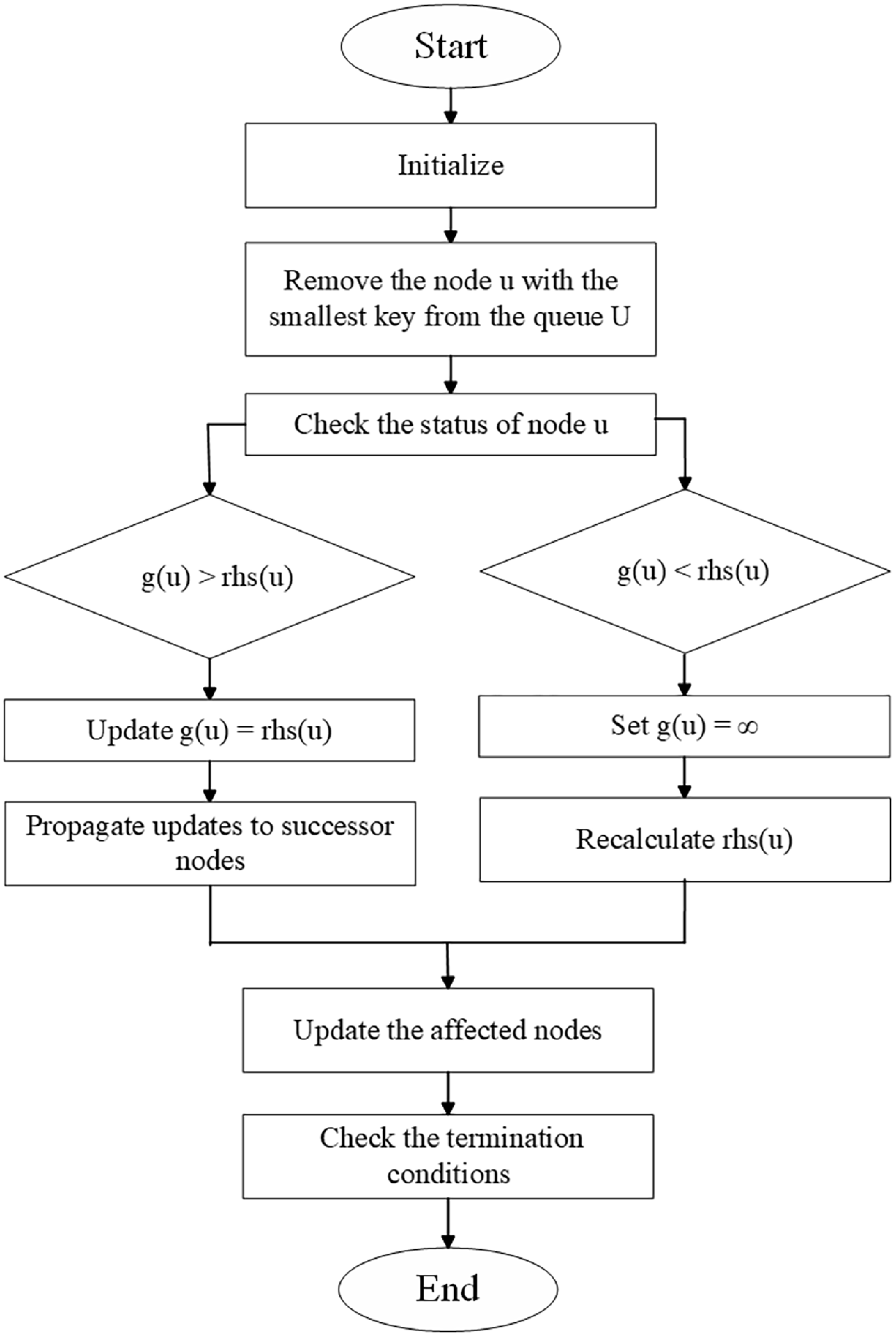
In dynamic environments, edge costs change due to events such as obstacle appearance or disappearance. When an edge cost changes, all nodes dependent on that edge are marked. For each affected node $u$ , its $rhs(u)$ is recalculated by function (2). If $rhs(u) \ne g(u)$ , node $u$ is inserted into priority queue $U$ , after which the $g$ and $rhs$ values of relevant nodes are recomputed until all nodes reach local consistency. The detailed workflow of the LPA* framework is shown in Figure 1.

Figure 1.

LPA* framework flow.

3.1. Dynamic heuristic strategy adjustment

The fixed heuristic function in the LPA* framework exhibits significant limitations in complex or dynamic environments. Firstly, it fails to adapt to intricate obstacle distributions, which potentially leads to suboptimal detours or local optima entrapment. Secondly, in scenarios with frequent dynamic obstacle changes, the static heuristic function cannot adjust in real time, which results in path conflicts. Local updates may trigger chain reactions, which require multiple iterations for convergence. Additionally, the inflexibility of this function hinders multi-objective optimization during path planning. Incremental update strategies may further trap paths in local optima, which necessitates additional computational corrections.

We replace the fixed heuristic function in the LPA* framework with Q-learning, designing the heuristic function as a weighted sum represented as

(3) \begin{equation} h(n) = {{\omega }_1} \cdot {h_{\textrm {distance}}}{(}n {) + } {\omega }_2 \cdot {h_{\textrm {obstacle}}}{(}n {) + } {\omega }_3 \cdot {h_{\textrm {smooth}}}{(}n {)}. \end{equation}

Here, ${\omega }_1$ , ${\omega }_2$ , and ${\omega }_3$ are weights dynamically adjusted by Q-learning, while ${h_{\textrm {diatance}}}{{(}}n{{)}}$ , ${h_{\textrm {obstacle}}}{{(}}n{{)}}$ , and ${h_{\textrm {smooth}}}{{(}}n{{)}}$ represent distinct heuristic action designs. ${h_{\textrm {diatance}}}{{(}}n{{)}}$ increases the weight on Euclidean distance to prioritize path length reduction. ${h_{\textrm {obstacle}}}{{(}}n{{)}}$ elevates the weight on obstacle distance to emphasize collision avoidance, and ${h_{\textrm {smooth}}}{{(}}n{{)}}$ augments the weight on path smoothness to reduce turning frequency.

We set the initial value of the distance weight $\omega _1$ as

(4)

where represents the Euclidean distance from the start point to the goal, while ${d_{\max }}$ denotes the diagonal distance of the map. The initial value of the obstacle weight $\omega _2$ is set as

(5) \begin{equation} {\omega _2} = \min (0.5,0.1 + 0.4 \cdot {p_{\textrm {obs}}}), \end{equation}

where $p_{\textrm {obs}}$ represents the obstacle density within the $3\times 3$ grid neighborhood centered at the start point. Therefore, the computational formula for the initial value of $\omega _3$ is

(6) \begin{equation} {\omega _3} = 1 - {\omega _1} - {\omega _2} \end{equation}

The weights $\omega _1$ , $\omega _2$ , and $\omega _3$ , dynamically adjusted via Q-learning, achieve adaptability to time-varying rewards. In open areas, the distance weight $\omega _1$ is prioritized to ensure the shortest path, while in narrow passages, the obstacle weight $\omega _2$ is increased to guarantee collision avoidance. This contextual adaptability prevents suboptimal detours caused by static, overly conservative obstacle avoidance strategies, effectively mitigating path oscillation issues.

To ensure the convergence of Q-learning, all state-action pairs must be visited infinitely often. In our policy, we employ the $\varepsilon$ -greedy strategy to balance exploration and exploitation. Additionally, the learning rate $\eta _t$ is denoted as

(7) \begin{equation} {\eta _t} = \frac {1}{{1 + t}}. \end{equation}

It decays according to function (4) and satisfies

(8) \begin{equation} \sum \limits _{t = 1}^\infty {{\eta _t}} = \infty ,\sum \limits _{t = 1}^\infty {\eta _t^2} \lt \infty . \end{equation}

After each path planning iteration, the error between the actual cost and the estimated cost is computed as

(9) \begin{equation} \Delta C = {C_{\textrm {actual}}} - {C_{\textrm {heuristic}}}. \end{equation}

We need to adjust the weights based on this function. If $\Delta C \gt 0$ , it indicates that the heuristic function underestimates the actual cost, which requires an increase in obstacle avoidance or smoothness weights. Conversely, if $\Delta C \lt 0$ , the heuristic overestimates the cost, which indicates the necessity to increase the distance weighting factor.

Using the L1 norm as the loss function, we obtain

(10) \begin{equation} L = \left | {\Delta C} \right |. \end{equation}

Compute the partial derivative with respect to weight ${{\omega }}_i$

(11) \begin{equation} \frac {{\partial L}}{{\partial {{{\omega }}_i}}} = \textrm {sign}(\Delta C) \cdot \frac {{\partial (\Delta C)}}{{\partial {{{\omega }}_i}}}. \end{equation}

By the chain rule, we obtain

(12) \begin{equation} \frac {{\partial (\Delta C)}}{{\partial {{{\omega }}_i}}} = \frac {\partial }{{\partial {{{\omega }}_i}}}\bigg({C_{\textrm {actual}}} - \sum \limits _j {{{{\omega }}_j}{h_j}} \bigg) = - {h_i}(n), \end{equation}

(13) \begin{equation} \frac {{\partial L}}{{\partial {{{\omega }}_i}}} = - \textrm {sign}(\Delta C) \cdot {h_i}(n). \end{equation}

The weight update rule is defined as

(14) \begin{equation} {{{\omega }}_i} = {{{\omega }}_i} - \beta \frac {{\partial L}}{{\partial {{{\omega }}_i}}}. \end{equation}

Substitute to get

(15) \begin{equation} {{{\omega }}_i} = {{{\omega }}_i} + \beta \cdot \textrm {sign}(\Delta C) \cdot {h_i}(n), \end{equation}

(16) \begin{equation} {{{\omega }}_i} = {{{\omega }}_i}{{ + }}\beta \cdot \textrm {sign(}\Delta C{{)}} \cdot \frac {{\partial h}}{{\partial {{{\omega }}_i}}}. \end{equation}

Here, $\beta$ is the learning rate for weight adjustment. This can be further simplified to

(17) \begin{equation} {\omega _i} = {\omega _i} + \beta \cdot \Delta C \cdot {h_i}(n). \end{equation}

Although any suboptimal path selection caused by noise will result in a large error after execution, this error is immediately fed back through the weight update rule, generating a strong correction signal, thereby ensuring that noise-induced errors are transient and are quickly corrected through the iterative process.

This iterative calibration process continuously minimizes the heuristic estimation error, ensuring that the search priorities of the LPA* algorithm dynamically adapt to multi-objective requirements such as path length, smoothness, and safety. This mechanism shifts the algorithm’s objective from a strict graph-search for the shortest path, which is prone to causing oscillations, toward kinematically optimal paths that are more suitable for physical robots.

Q-learning learns optimal weight combinations across environments through trial-and-error. Specifically, in open-area scenarios, prioritizing the distance weight ${{\omega }}_1$ shortens path lengths. In narrow-channel scenarios, increasing the obstacle weight ${{\omega }}_2$ prevents collisions. While the LPA* framework establishes a global path framework, Q-learning locally optimizes paths via dynamic weight adjustments. Concurrently, closed-loop error feedback computes $\Delta C$ from actual path execution outcomes, then iteratively adjusts weights through error backpropagation to reduce heuristic estimation errors progressively.

Additionally, Q-learning improves real-time performance by dynamically adjusting LPA*’s update policies to reduce redundant computations. The state vector is defined as

(18) \begin{equation} s = \left[{f_{\textrm {change}}},{p_{\textrm {collision}}},{N_{\textrm {local}}},\eta \right], \end{equation}

where $f_{\textrm {change}}$ denotes the environment change frequency, calculated as the ratio of environmental change occurrences to the time window duration. $p_{\textrm {collision}}$ represents the path conflict probability, calculated as the ratio of recent collision instances to path update attempts. $N_{\textrm {local}}$ indicates the historical local update count, while $\eta$ is the ratio of the current path cost to the optimal cost.

Regarding the reward mechanism, we set the computational efficiency reward as

(19) \begin{equation} {r_{\textrm {efficiency}}} = \rho \cdot \left(1 - \frac {{{t_{\textrm {new}}}}}{{{t_{\textrm {old}}}}}\right), \end{equation}

where $t_{\textrm {old}}$ and $t_{\textrm {new}}$ denote the computation time before and after strategy adjustment, and $\rho$ is the reward coefficient. If an action reduces computation time, the reward is proportional to the time saved. If an action increases path cost, the penalty is set as

(20) \begin{equation} {r_{\textrm {penalty}}} = - \kappa \cdot \left(\frac {c_{\textrm {new}} - c_{\textrm {old}}} {c_{\textrm {old}}}\right), \end{equation}

$c_{\textrm {old}}$ and $c_{\textrm {new}}$ represent the costs before and after strategy adjustment, respectively. $\kappa$ is the reward coefficient, and the total reward function is

(21) \begin{equation} r = {r_{\textrm {efficiency}}} + {r_{\textrm {penalty}}}. \end{equation}

The update policy mapping for LPA* divides the action execution logic into three strategies. The first strategy ( $a_1$ ), which updates only the first-order neighbors of the affected nodes, incurs the minimal computational cost. The second ( $a_2$ ) strategy updates second-order neighbors to balance update scope. The third strategy ( $a_3$ ) resets the OPEN list to activate global A* search. Q-learning perceives environmental dynamics and algorithm states through state $s$ , while regulating the update scope of LPA* by selecting action $a$ . In low-dynamic environments with small $f_{\textrm {change}}$ values, action $a_1$ is prioritized to reduce computational overhead. In high-dynamic environments with large $f_{\textrm {change}}$ values, action $a_3$ is selected for global replanning to prevent local updates from entering infinite loops. When path quality deteriorates( $\eta \gt 1.2$ ), action $a_3$ is enforced to escape local optima.

3.2. Incremental experience reuse

Q-learning, a trial-and-error-based reinforcement learning method, faces core challenges in efficiently exploring and identifying optimal policies within complex or high-dimensional environments. In unknown environments, Q-learning requires extensive random exploration, which results in slow convergence and low sample efficiency. LPA*, as an incremental path planning framework, generates and maintains global paths in dynamic environments. By leveraging its output path nodes and cost information as prior knowledge, LPA* significantly accelerates Q-learning’s learning process.

During path planning with the LPA* framework, the generated global path comprises a sequence of nodes denoted as $N = \left \{ {{n_1},{n_2},{n_3},\ldots ,{n_k}} \right \}$ , where each node $n$ contains positional coordinates and path cost information. LPA* maintains the minimum path cost $C_{\min }$ from the start to the goal while calculating the heuristic estimate $h({n_i})$ representing the remaining cost from each node $n_i$ to the target. We integrate LPA*’s path nodes with real-time environmental data to define the state vector as

(22) \begin{equation} s = \left[{x_{\textrm {robot}}},{x_{\textrm {goal}}},\left \{ {h({n_i})} \right \}_{i = 1}^k,\textrm {od}\right], \end{equation}

where $x_{\textrm {robot}}$ represents the robot’s current position. $x_{\textrm {goal}}$ denotes the target position, and $\textrm {od}$ quantifies obstacle distribution. We replace Q-learning’s original action space with the path node set $N$ provided by the LPA* framework and define $A = N$ as the new candidate action set. During action selection, Q-learning chooses action $a \in A$ under state $s$ , corresponding to moving to a specific path node $n_i$ . When successfully reaching node $n_i$ , the reward is proportional to the reduction ratio of path cost, expressed as

(23) \begin{equation} {r_{\textrm {reach}}} = \lambda \cdot \left(1 - \frac {{C({n_i})}}{{{C_{\min }}}}\right), \end{equation}

where $\lambda$ represents the reward coefficient for node arrival, and $C({n_i})$ denotes the actual navigation cost from the current position to node $n_i$ . The path cost $C_{\min }$ from LPA* serves as the reward benchmark for Q-learning. When $C({n_i}) \lt {C_{\min }}$ (indicating an optimized path), the agent receives higher rewards. Conversely, when $C({n_i}) \gt {C_{\min }}$ (signifying suboptimal path quality), the system reduces rewards or triggers penalties.

Additionally, a global goal proximity reward is introduced, which grants extra rewards when approaching the final target. The reward is defined as

(24) \begin{equation} {r_{\textrm {goal}}} = \varphi \cdot \bigg(1 - \frac {{ \| { {{x_{\textrm {robot}}}} - {x_{\textrm {goal}}} \|} }}{{\| {{{x_{\textrm {start}}}} - {x_{\textrm {goal}}} \|} }}\bigg), \end{equation}

where $\varphi$ represents the global goal proximity reward coefficient. Importantly, a collision penalty $r_{\textrm {collision}}$ ( ${r_{\textrm {collision}}} \lt 0$ ) is imposed if the agent collides during movement. Therefore, the total reward function can be represented as

(25) \begin{equation} r = {r_{\textrm {reach}}} + {r_{\textrm {goal}}} + {r_{\textrm {collision}}}. \end{equation}

To enhance efficiency and ensure robust path planning during agent navigation, dynamic node maintenance is implemented through two mechanisms. Node pruning refers to the process where nodes are deprioritized or removed from the graph structure due to prolonged inactivity or collision risks. Dynamic node addition is the process triggered by the LPA* framework’s detection of a new path. Following this, the relevant nodes are integrated into set, and the Q-learning action space is updated.

The node sequence generated by LPA* provides structured exploration guidance for Q-learning, while the heuristic cost $h({n_i})$ assists Q-learning in evaluating node priorities to favor those closer to the goal. Q-learning’s action space is compressed by a continuous high-dimensional domain to a discrete set of path nodes, which significantly reduces exploration complexity and avoids inefficient search patterns. When environmental changes occur, LPA* updates the path node queue and prompts Q-learning simultaneously adjust its action space, which ensures that prior knowledge remains consistently valid.

After environmental changes trigger LPA* replanning, Q-learning immediately acquires updated global knowledge, avoiding inefficient random exploration. The updated path node sequence $N$ generated by LPA* is used as the initial subgoal set for Q-learning. This structured guidance minimizes redundant search and accelerates the convergence of Q-learning.

3.3. Discretization of high-dimensional action spaces

Q-learning is confronted with the curse of dimensionality in high-dimensional continuous action spaces, where the action space size grows exponentially with dimensionality, rendering memory and computational resources insufficient to support storage and processing demands. Furthermore, random exploration in continuous spaces requires excessive samples, which leads to low sample efficiency, slow convergence rates, and difficulties in discovering globally optimal actions while becoming trapped in local optima. LPA* naturally generates a discrete candidate action set by operating within the continuous space to produce path nodes. This integration of path nodes as Q-learning’s discrete action space significantly reduces computational complexity while preserving the feasibility and optimality of path planning solutions.

When the LPA* algorithm operates in continuous space ${\delta }$ for path generation, with path nodes $N$ forming a low-dimensional discrete subspace, the equivalence $N \subset {{\delta }}$ holds under subspace dimensionality constraints. By compressing Q-learning’s action space from ${\delta }$ to $N$ , the computational complexity is reduced from exponential $O({N^d})$ to linear $O(K)$ with $K = \left | N \right |$ . This discrete action space $A = N$ enables Q-learning to cover all state-action pairs in polynomial time, satisfying the convergence requirement

(26) \begin{equation} \mathop {\lim }\limits _{t \to \infty } {Q_t}(s,a) = {Q^*}(s,a). \end{equation}

The design logic of the reward function can be inferred from the discussion in section 3.2. The reward component $r_{\textrm {reach}}$ incentivizes the selection of path-shortening nodes to optimize path costs, while the penalty term $r_{\textrm {collision}}$ suppresses hazardous actions to ensure safety. Concurrently, the goal-oriented reward $r_{\textrm {goal}}$ accelerates convergence toward the target. To enhance decision efficiency, node prioritization is implemented through a priority weight dynamically adjusted during exploration, defined as

(27) \begin{equation} w({n_i}) = \frac {1}{{C({n_i}) + {{\mu }}}}, \end{equation}

where ${\mu }$ serves as a small constant to prevent division-by-zero errors. Q-learning samples actions proportionally to their weights, and thus prioritizes high-quality nodes during selection. Path nodes are dynamically generated by LPA* to satisfy obstacle avoidance and kinematic constraints, which prevents Q-learning from selecting infeasible actions. When the environmental changes occur, LPA* updates the node queue, which maintains real-time validity of the action space while ensuring persistent compliance with safety and motion feasibility requirements.

Figure 2.

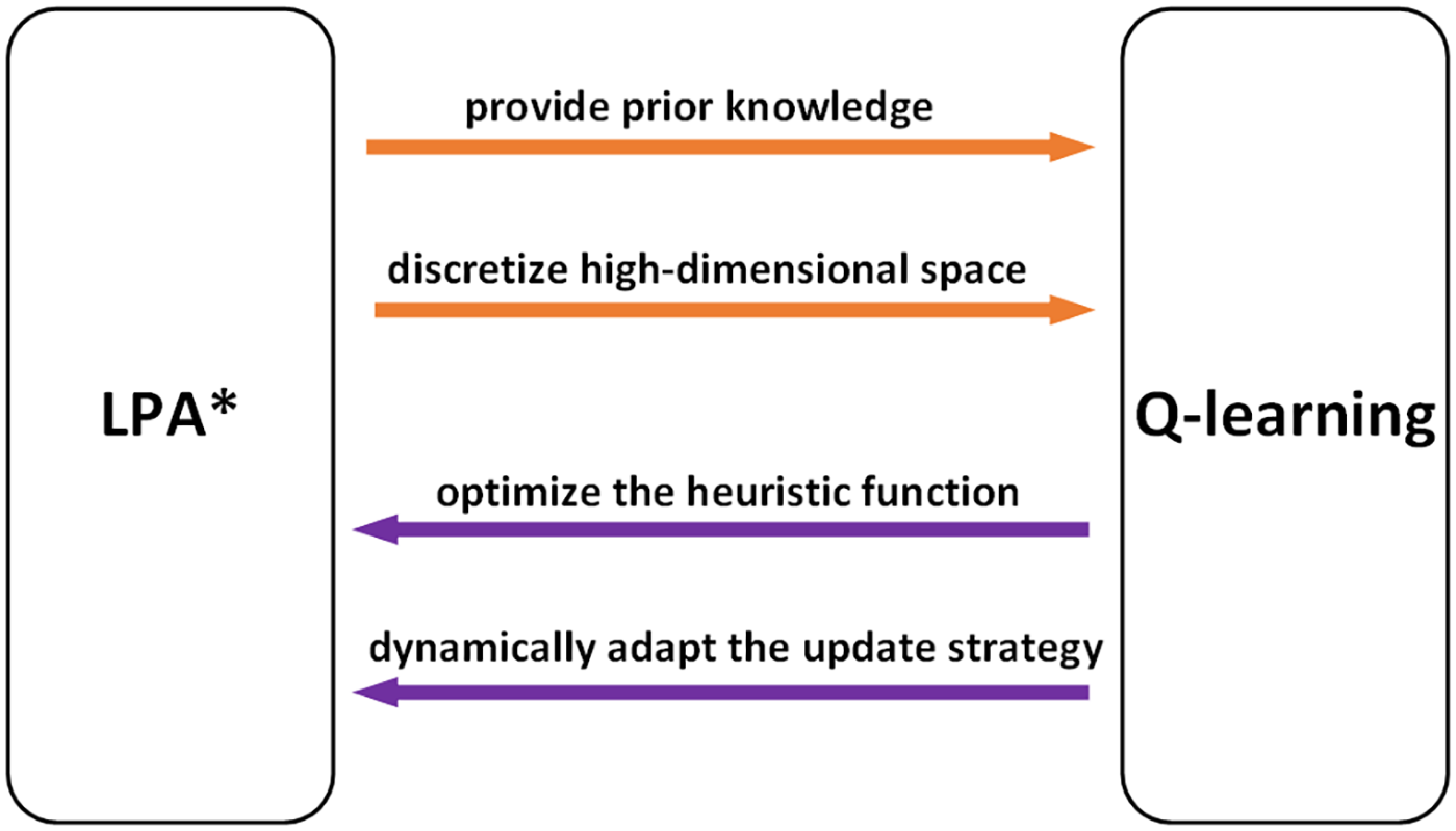
Schematic diagram of bidirectional optimization.

3.4. Algorithm design and complexity analysis

Although many details of bidirectional optimization have been described in previous sections, to better explain the process of bidirectional optimization, we have prepared Figure 2.

As shown in Figure 2, LPA* optimizes Q-learning mainly in two aspects: providing prior knowledge and discretizing high-dimensional space. In unknown environments, Q-learning requires extensive random exploration, resulting in slow convergence and low sample efficiency. The incremental nature of LPA* ensures its ability to generate and maintain global paths in dynamic environments. Its output (path nodes and cost information) serves as prior knowledge, significantly accelerating Q-learning’s learning process. Simultaneously, Q-learning struggles to find optimal paths in high-dimensional action spaces. Mapping continuous space to LPA*-generated finite path nodes avoids the expansion of high-dimensional action spaces and reduces action space dimensionality.

Q-learning optimizes LPA* primarily in two aspects: optimizing the heuristic function and dynamically adapting the update strategy. The fixed heuristic function of LPA* cannot adapt to complex obstacle distributions, potentially causing circuitous paths or local optima entrapment. Simultaneously, in scenarios with frequent dynamic obstacle changes, fixed heuristics cannot adjust in real-time, leading to path conflicts and chain reactions from local updates that require multiple iterations to converge. Q-learning redesigned the heuristic function as a weighted sum, ensuring optimization of estimation accuracy through feedback mechanisms. Furthermore, Q-learning dynamically adjusts LPA*’s update strategy based on environmental characteristics in real-time, avoiding unnecessary local updates and enhancing path quality.

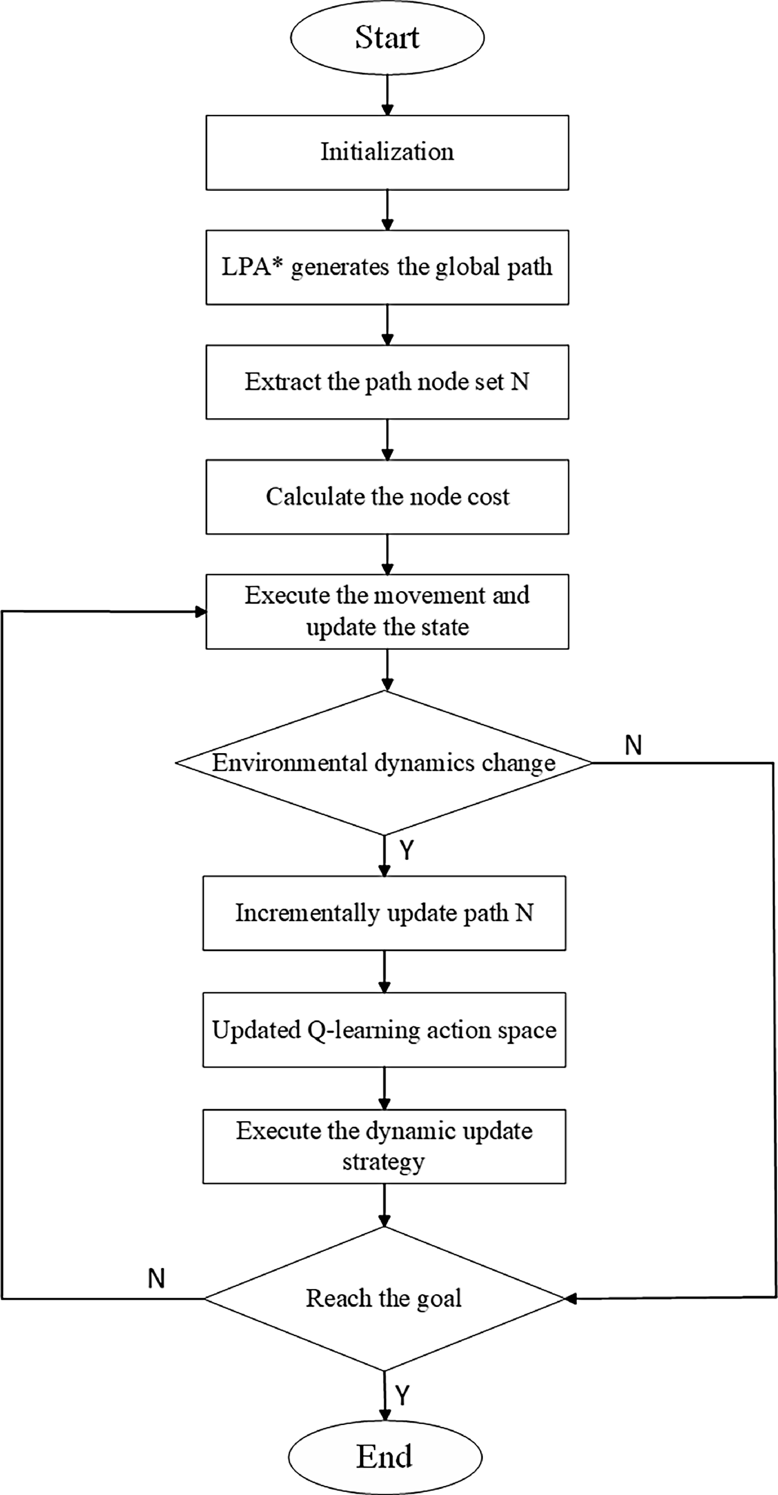
The operational sequence of the BQ-LPA* algorithm is illustrated in Figure 3. Following parameter initialization, it first generates a global path based on LPA* and computes the remaining cost estimate from each waypoint to the goal to accelerate Q-learning convergence. Subsequently, it executes moves and updates states according to our designed heuristic function. When environmental dynamics change, the algorithm incrementally updates path $N$ using LPA* and expands Q-learning’s action space. Concurrently, our dynamic update strategy activates to eliminate redundant computations and enhance real-time performance. These procedures iterate iteratively until the destination is reached.

Figure 3.

BQ-LPA* algorithm flow.

We now analyze the time complexity and space complexity of BQ-LPA*.

Time complexity: In the classic LPA*, the time complexity is primarily determined by the number of updated nodes $U$ and the total number of nodes $V$ , typically represented as $O(U\log V)$ , where $log V$ arises from priority queue operations. In classic Q-learning, the time complexity is $O(N \cdot A)$ , where $N$ is the number of states and $A$ is the number of actions. In BQ-LPA*, since Q-learning optimizes the heuristic function and update strategy, $U$ is further reduced, denoted as $U'$ ( $U' \ll U$ ). Simultaneously, LPA* reduces the effective state-action pairs for Q-learning by narrowing the action space (via discretization of high-dimensional spaces) and providing global path guidance, resulting in reduced $N'$ and $A'$ ( $N' \ll N$ , $A' \ll A$ ). Thus, the overall time complexity of BQ-LPA* is $O(U'\log V + N' \cdot A')$ .

Space complexity: In the classic LPA*, the space complexity is also primarily determined by the number of updated nodes $U$ and the total number of nodes $V$ , typically expressed as $O(V + U)$ , approximately $O(V)$ . In classic Q-learning, the space complexity is $O(N \cdot A)$ , where $N$ is the number of states and $A$ is the number of actions. In BQ-LPA*, since LPA* provides prior knowledge and refines the action space for Q-learning, the number of effective state-action pairs is reduced to $N'$ and $A'$ ( $N' \ll N$ , $A' \ll A$ ). Therefore, the overall space complexity of BQ-LPA* is $O(V) + O(N' \cdot A')$ .

Through action space dimensionality reduction, incremental experience reuse, and improvements to heuristics and update strategies, BQ-LPA* significantly enhances its practical feasibility and scalability in complex dynamic environments while reducing complexity.

4.1. Simulation experiment setup

To validate the advantages of the BQ-LPA* algorithm in path planning, simulations are conducted under the following configurations. The hardware platform utilizes a Windows 11 operating system with an Intel Core i7-13650H processor operating at a base frequency of 2.60 GHz and 16 GB of RAM. MATLAB 2023b serves as the simulation environment. The grid map used in the simulation consists of square cells with a unit length of 1, where white areas designate traversable regions and black areas represent obstacles. In Q-learning, $\alpha$ is the learning coefficient, and reflects the degree to which the previous Q-value is retained. $\alpha$ is set to 0.2 in our study. The variable $\gamma$ is the discount factor, which represents the degree of importance an agent attaches to future rewards when it receives the current reward, and it is set to 0.8 [Reference Khriji, Touati, Benhmed and Al-Yahmedi27]. The replanning threshold for the LPA* algorithm is set at 0.3, meaning replanning is triggered when environmental changes exceed 30%. The heuristic scaling factor is configured to 1.2, which effectively achieves a balance between path quality and computational efficiency.

4.2. Comparative analysis of dynamic heuristic strategy adjustments

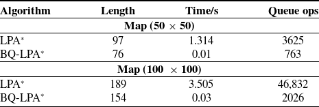
As described in Section 3.1, BQ-LPA* employs Q-learning to optimize the fixed heuristic function and update strategy of LPA*, enhancing estimation accuracy through a feedback mechanism. To verify its reliability, simulation comparisons are conducted between the classical LPA* algorithm and the proposed BQ-LPA* algorithm using 50 $\times$ 50 and 100 $\times$ 100 grid maps, with obstacle density set to 0.25. Both algorithms are configured with a starting point at (1, 1) and goals at (50, 50) and (100, 100) for the respective map sizes. The number of iterations for BQ-LPA* is 1000. The path planning results are shown in Figures 4 and 5, and the relevant data are presented in Table I.

Figure 4.

Comparative results of dynamic heuristic strategy adjustments under 50 $\times$ 50.

Figure 5.

Comparative results of dynamic heuristic strategy adjustments under 100 $\times$ 100.

As shown in Figures 4 and 5, classic LPA* generated paths with unnecessary detours and zigzag patterns across both grid map scales due to obstacle circumvention strategies. These redundant maneuvers inevitably increase energy consumption and travel duration during robot navigation. In contrast, BQ-LPA* produced significantly streamlined trajectories that directly target subgoals, which proves more efficient in practical scenarios by minimizing redundant path segments and reducing planning costs.

The data listed in Table I reveal that the BQ-LPA* algorithm reduces planned path lengths by 18.5% to 23.2% compared to the classic LPA* algorithm. This improvement stems from its Q-learning-integrated reward mechanism, which prioritizes straight-line paths and minimizes redundant turns. Queue operations refer to the cumulative actions of inserting, extracting, and deleting nodes in the priority queue during algorithm execution, which directly impact computational efficiency and serve as a critical performance indicator. Higher operation counts increase computational resource consumption and degrade replanning agility in dynamic environments.

While the classic LPA* suffers computational explosions due to frequent queue operations, BQ-LPA* leverages Q-learning’s incremental learning to drastically reduce inefficient node expansions. Consequently, queue operation counts are reduced by 78.9 and 95.7% for the 50 $\times$ 50 and 100 $\times$ 100 maps. This substantial decrease confirms that the optimization of the LPA* update strategy by Q-learning is successful, avoiding update chain reactions, thereby reducing the average planning time by more than 90% compared to the classical LPA*.

Table I.

Simulation data of dynamic heuristic strategy adjustments.

4.3. Comparative analysis of dynamic adaptability

As detailed in sections 3.2 and 3.3, the BQ-LPA* algorithm leverages prior knowledge provided by LPA* to accelerate Q-learning convergence while mitigating inefficient exploration. By discretizing continuous spaces, it also resolves Q-learning’s high-dimensional action selection challenges. To validate these advantages, simulations of Q-learning and BQ-LPA* are conducted on a 50 $\times$ 50 grid map. The starting point of the planning map for Q-learning and BQ-LPA* is set to (1,1), the endpoint to (50,50), with obstacle density set to 0.25.

Figure 6.

Comparative results of dynamic adaptability under 50 $\times$ 50.

Table II.

Simulation data in various dynamic environments.

The path planning result of Q-learning and BQ-LPA* is shown in Figure 6, which is generated within an identical grid-based simulation environment to ensure fairness. The BQ-LPA* algorithm generates notably shorter paths with fewer detours and angular deviations, attributable to its integration of LPA*-derived prior knowledge that accelerates convergence and minimizes unproductive exploration.

Additionally, to test the path planning capability of BQ-LPA* in dynamic environments, we configure three dynamic environments for simulation testing. We still implement dynamic configurations based on the 50 $\times$ 50 grid map with obstacle density set to 0.25. Regarding collision behaviors of dynamic obstacles, we establish specific protocols. A dynamic obstacle automatically reverses direction upon reaching its path endpoint. When encountering static obstacles during movement, it immediately reverses to simulate wall-bouncing behavior. Dynamic obstacles neither perform mutual avoidance nor collide with each other. They are permitted to pass through one another to maintain motion continuity.

Low-dynamic environment: The objective is to test the algorithm’s fundamental obstacle avoidance and path fine-tuning capabilities for small quantities of predictable dynamic obstacles. Among 625 obstacle cells, we configure 10 dynamic obstacles moving at a constant low speed of 0.5 grid cells per second. This quantity sufficiently introduces dynamism without causing excessive map congestion. Each dynamic obstacle moves along a predetermined linear path and then reverses direction in a continuous loop.

Medium-dynamic environment: The objective is to test the algorithm’s replanning and local obstacle avoidance capabilities in moderately congested environments with stochastic obstacle behaviors. We configure 25 dynamic obstacles whose velocities are not constant but randomly selected within the range of 1.0 to 2.0 grid cells per second. This results in localized congestion requiring more frequent replanning by the algorithm. Each dynamic obstacle still moves along a predetermined linear path and then reverses direction in a continuous loop.

High-dynamic environment: The objective is to evaluate the algorithm’s real-time decision-making and high robustness in dense, complex, and unpredictable dynamic environments. We configure 50 dynamic obstacles with velocities randomly selected between 0.5 and 3.0 grid cells per second. This creates severe map congestion simulating high-traffic scenarios, requiring efficient real-time local obstacle avoidance. At simulation start, each obstacle randomly selects a traversable grid cell as its target point and moves toward it at constant speed. Upon reaching the target, it briefly pauses before selecting a new random target point and repeating the process.

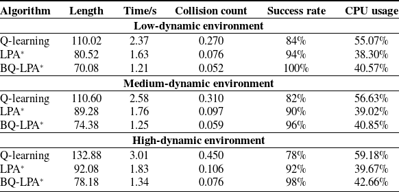
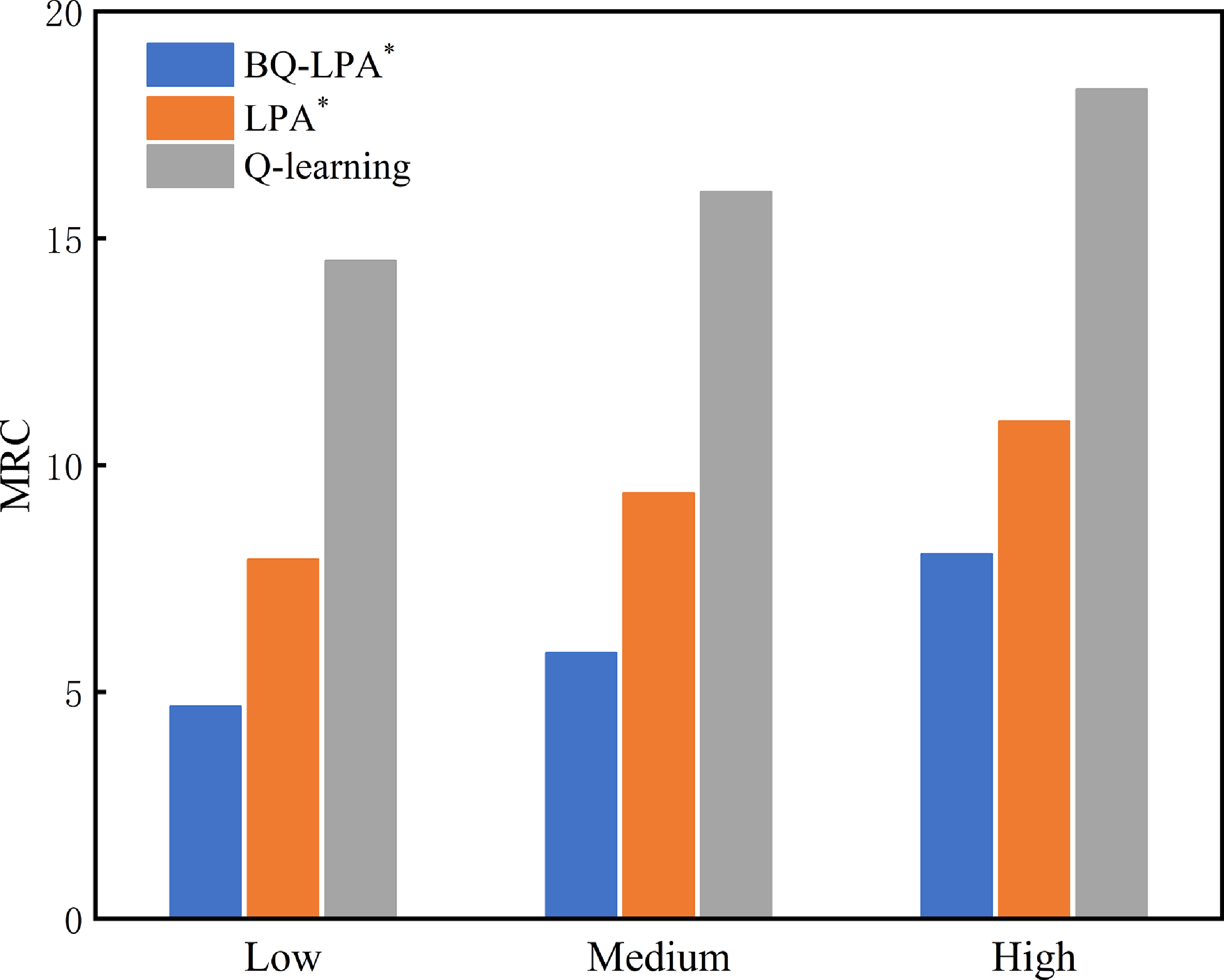
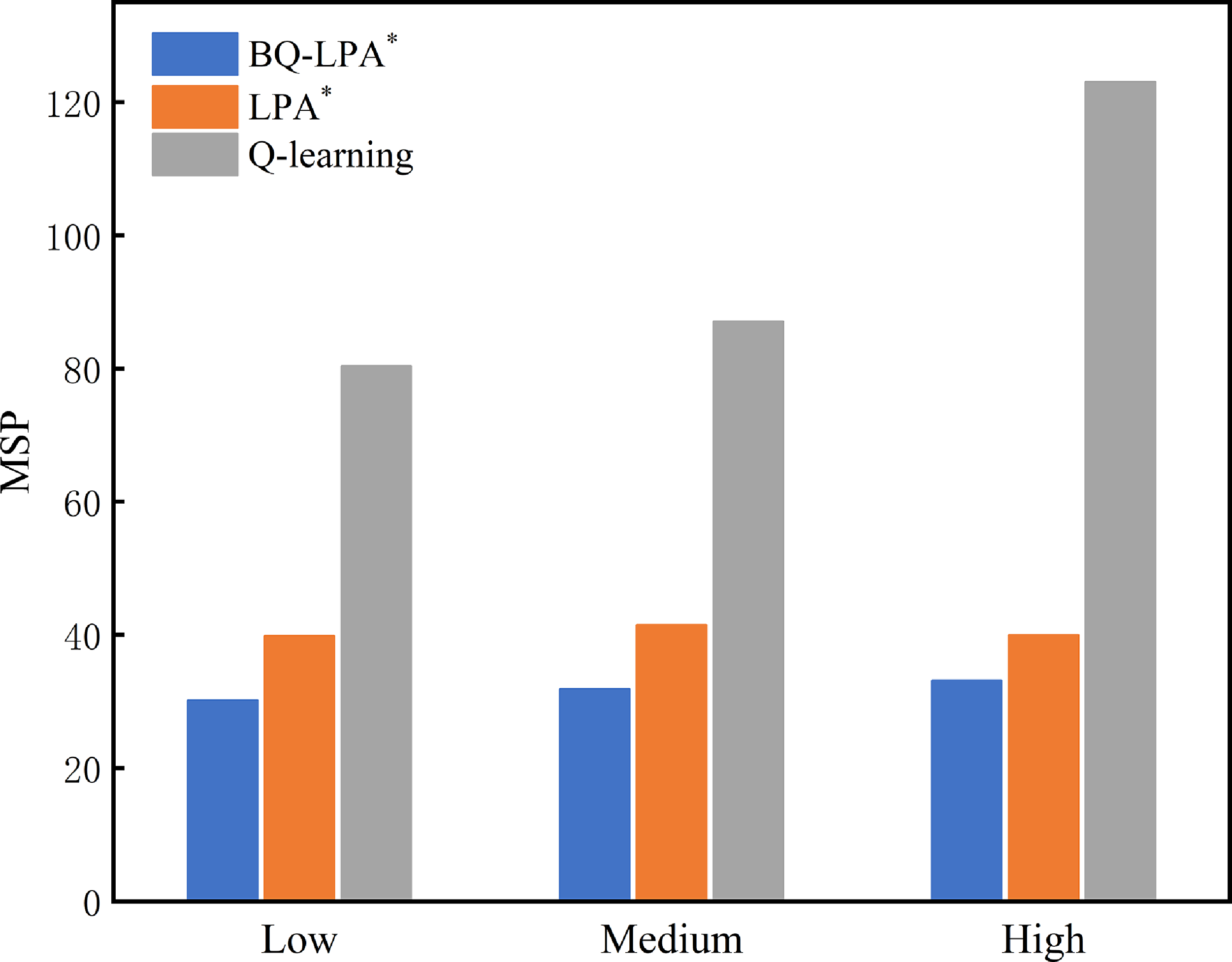
For Q-learning, LPA*, and BQ-LPA*, simulation experiments consisting of 50 runs each are conducted in the aforementioned three dynamic environments. The average results of multiple metrics over 50 rounds are presented in Table II, while Figures 7 and 8, respectively, illustrate the comparative performance of the three algorithms regarding mean replanning count (MRC) and mean suboptimality percentage (MSP) across different dynamic environments.

Replanning count refers to the number of times an algorithm recalculates its path during the entire journey from start to goal due to the emergence or positional changes of dynamic obstacles. This metric reflects the algorithm’s real-time performance and computational overhead. A higher replanning count indicates more frequent responses to environmental changes, but simultaneously implies greater computational burden. Suboptimality percentage measures the deviation between the path generated by the algorithm and the theoretically optimal path (typically the shortest path in static environments). This metric primarily evaluates path efficiency in dynamic environments. A lower suboptimality percentage signifies that the algorithm effectively navigates around dynamic obstacles while maintaining minimal detours, thus preserving near-optimal path length.

Figure 7.

Comparison of mean replanning count in different dynamic environments.

Figure 8.

Comparison of mean suboptimality percentage in different dynamic environments.

BQ-LPA* achieves planning success rates exceeding 96% across diverse dynamic environments, even attaining 100% in low-dynamic environments. This underscores its exceptional mission completion reliability under varying environmental conditions. In terms of path efficiency metrics, BQ-LPA* demonstrates the shortest mean path length and lowest mean collision count, validating its superior capability in generating highly efficient collision-free trajectories. The algorithm’s lower replanning count and suboptimality percentage further substantiate the effectiveness and optimality of its path planning capabilities. Notably, as environmental complexity intensifies, both planning time and CPU usage exhibit only marginal increases while consistently maintaining low levels. This confirms BQ-LPA*’s robust adaptability to high-frequency environmental perturbations, sustaining computationally efficient replanning with minimal resource consumption.

LPA* also maintains relatively high success rates across diverse environments. However, compared to BQ-LPA*, it exhibits higher values in metrics including mean step count, collision count, replanning count, and suboptimality percentage, along with more significant time consumption. This confirms that while LPA*’s incremental planning mechanism remains effective in dynamic environments, its path efficiency and computational efficiency are inferior to BQ-LPA*.

Q-learning struggles even in mildly dynamic environments, achieving only an 84% success rate while exhibiting high collision count, elevated replanning count, and excessive CPU usage. This indicates its failure to converge toward near-optimal solutions for dynamic path planning tasks, suggesting potential issues such as prohibitive exploration costs or slow convergence rates. As environmental complexity escalates, its learning process cannot keep pace with rapid environmental changes, demonstrating an inability to learn effective strategies. Such performance makes Q-learning unsuitable for real-time dynamic path planning applications.

The integration of prior knowledge from LPA* significantly enhances BQ-LPA*’s convergence rate and path quality. During environmental changes, LPA* dynamically updates the node set to maintain the real-time validity of the action space, while the discretized action space ensures comprehensive coverage of all state-action pairs within bounded time frames. This guarantees the algorithm’s convergence criteria. By deeply integrating adaptive LPA* with Q-learning, the hybrid framework achieves an optimal balance between planning efficiency and solution quality, which provides an effective decision-making solution for autonomous systems operating in complex dynamic environments.

4.4. Comparative analysis of multiple path planning algorithms

To validate the planning capability of the BQ-LPA* algorithm in a real-world environment, we select an authentic environmental map, which is made publicly available by Hidalgo-Paniagua et al. [Reference Hidalgo-Paniagua, Vega-Rodríguez, Ferruz and Pavón28]. The map is illustrated in Figure 9, with Figure 9(a) showing the original real-world scene and Figure 9(b) displaying the rasterized map after grid processing.

Figure 9.

An authentic environmental map.

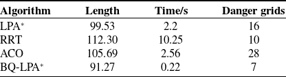
We removed Q-learning, which performed poorly in Section 4.3, and incorporated two mainstream path planning algorithms, RRT and ACO. In the aforementioned real-world environment, we conducted 50 simulation experiments and selected the best-performing results for each algorithm. The specific path planning outcomes are illustrated in Figure 10, with relevant data recorded in Table III.

Table III.

Simulation data of multiple path planning algorithms in the authentic environment.

Figure 10.

Comparative results of multiple path planning algorithms.

As shown in Figure 10, the RRT algorithm connects multiple randomly sampled nodes, which results in a path with pronounced randomness that appears tortuous and non-smooth. Notably, when avoiding obstacles, it generates numerous sharp turns that substantially reduce path planning efficiency. The ACO-produced path is smoother than RRT’s, but still exhibits noticeable curvature and appears less direct than LPA* or BQ-LPA*. It also detours around the central obstacle with a longer route resembling RRT’s approach, yet less pronounced, while adhering more closely to obstacle contours in certain regions. The path generated by LPA* appears relatively direct and navigates the environment efficiently, successfully traversing the cluttered central area. This path features several abrupt, orthogonal turns, which is a characteristic feature of grid-based search algorithms moving along grid lines. BQ-LPA* produces the most direct, smooth, and visually efficient path. It traverses the central zone with minimal detours, executing gentler turns than LPA*, demonstrating exceptional effectiveness in identifying optimal collision-free trajectories. According to Table III, BQ-LPA* achieves the shortest path length and fastest planning speed among all algorithms, showcasing superior planning efficiency.

In our study, A grid is classified as dangerous if the distance between an obstacle and the planned path falls below a predefined threshold (set at 0.25). Fewer danger grids indicate fewer unsafe segments along the path, resulting in enhanced overall safety. Specifically, BQ-LPA* reduces danger grids by over 50% compared to the relatively efficient LPA*, and achieves a 75% reduction versus ACO, which exhibits moderate obstacle avoidance. Although RRT’s danger grid count approaches BQ-LPA*’s, this safety improvement entails disproportionately longer paths, representing an impractical trade-off. These results demonstrate that through obstacle weighting and collision penalties, BQ-LPA* not only effectively mitigates collision risks but also outperforms mainstream algorithms in both planning efficiency and computational complexity.