1. Introduction
Internal waves at tidal frequencies, known as internal tides, are a prominent source of energy available for vertical mixing in the deep ocean. Such internal-tide-driven mixing is an important consideration for understanding the large-scale ocean circulation and the global energy budget (Munk & Wunsch Reference Munk and Wunsch1998; Wunsch & Ferrari Reference Wunsch and Ferrari2004). Large-scale ocean models parameterise internal tide generation, their subsequent evolution, dissipation and the vertical mixing they drive (MacKinnon et al. Reference MacKinnon2017; Whalen et al. Reference Whalen, De, Casimir, Alberto, Klymak, MacKinnon and Sheen2020). As a result, simple yet accurate models to understand and quantify these internal-tide-related processes are crucial for the improvement of ocean models whose grids lack the resolution to explicitly capture them. From a fluid mechanics viewpoint, nonlinear processes, such as intensified boundary flows, wave breaking, wave–wave interactions and instabilities in internal wave beams, can drive topographic internal waves towards turbulence (Sarkar & Scotti Reference Sarkar and Scotti2017) and the enhanced mixing that accompanies it. In this paper, we study tide–topography interaction to model simultaneous generation and scattering of internal waves by isolated deep ocean ridges, and present a potential mechanism that can act as a pathway towards the aforementioned nonlinear processes.
Of the 2.4 TW of semi-diurnal (M2) tidal energy dissipated in the oceans, around 1 TW is attributed to barotropic-to-baroclinic conversion into internal waves (Egbert & Ray Reference Egbert and Ray2001; Nycander Reference Nycander2005). Most of this conversion occurs in regions with significant bottom topography, including continental shelves (Lamb Reference Lamb2014) and isolated tall features (Merrifield, Holloway & Johnston Reference Merrifield, Holloway and Johnston2001; Alford et al. Reference Alford2015). To estimate internal tide generation in the deep ocean, two-dimensional linear models that consider a barotropic oscillatory flow over bottom topography have been useful (Garrett & Kunze Reference Garrett and Kunze2007). Such models vary in the range of assumptions they make, particularly in terms of the topographic height and slope, the ocean depth and the stratification profile (Bell Reference Bell1975; Bell Jr Reference Bell1975; Llewellyn Smith & Young Reference Smith, Stefan and Young2002; Balmforth, Ierley & Young Reference Balmforth, Ierley and Young2002; Laurent et al. Reference Laurent, Stringer, Garrett and Perrault-Joncas2003; Balmforth & Peacock Reference Balmforth and Peacock2009). The Green function approach has emerged as a powerful tool that can account for arbitrary two-dimensional topographic shapes in a non-uniformly stratified finite-depth fluid (Pétrélis et al. Reference Pétrélis, Smith and Young2006; Echeverri & Peacock Reference Echeverri and Peacock2010; Mathur, Carter & Peacock Reference Mathur, Carter and Peacock2016). While these linear modelling efforts have provided useful qualitative and quantitative insights into internal tide generation and its characteristics, some of the underlying physics are still not well understood. For example, a combination of theoretical, numerical and experimental studies has shown that the topographic slope relative to the internal wave ray slope (Zhang, King & Swinney Reference Zhang, King and Swinney2008; Gayen & Sarkar Reference Gayen and Sarkar2011; Papoutsellis, Mercier & Grisouard Reference Papoutsellis, Mercier and Grisouard2023), the topographic height (Zhao, Zhang & Swinney Reference Zhao, Zhang and Swinney2015) and its specific shape (Legg & Adcroft Reference Legg and Adcroft2003; Maas Reference Maas2011) can non-trivially influence internal tide generation.
An overall summary of satellite observations and modelling of internal tide generation is that coherent low-mode internal tides travel far from their generation sites (Ray & Mitchum Reference Ray and Mitchum1997; Zhao & Alford Reference Zhao and Alford2009), while the high-mode content dissipates in the near field (Garrett & Kunze Reference Garrett and Kunze2007). Internal tide scattering by bottom topography has been proposed as a mechanism through which far-propagating low-mode internal tides could lose their energy to higher modes and ultimately dissipate (Johnston & Merrifield Reference Johnston and Merrifield2003; Johnston, Merrifield & Holloway Reference Johnston, Merrifield and Holloway2003; Nash et al. Reference Nash, Kunze, Toole and Schmitt2004; Lahaye, Gula & Roullet Reference Lahaye, Gula and Roullet2020; Li & Xie Reference Li and Xie2023). Modelling efforts (analytical, numerical and experimental) have therefore investigated the scattering of low-mode internal waves by isolated and small-amplitude random topographies (Müller & Xu Reference Müller and Xu1992; Müller & Liu Reference Müller and Liu2000; Peacock et al. Reference Peacock, Mercier, Didelle, Viboud and Dauxois2009; Bühler & Holmes-Cerfon Reference Bühler and Holmes-Cerfon2011; Legg Reference Legg2014; Mathur, Carter & Peacock Reference Mathur, Carter and Peacock2014; Li & Mei Reference Li and Mei2014). These studies have shown that near-critical and supercritical isolated topographies, and large extents of small-scale random topography, can efficiently scatter low-mode internal wave energy to higher modes. As for the modelling of internal tide generation by bottom topography, the Green function approach has proven to be useful for topographic scattering studies too (Robinson Reference Robinson1969; Mathur et al. Reference Mathur, Carter and Peacock2014).
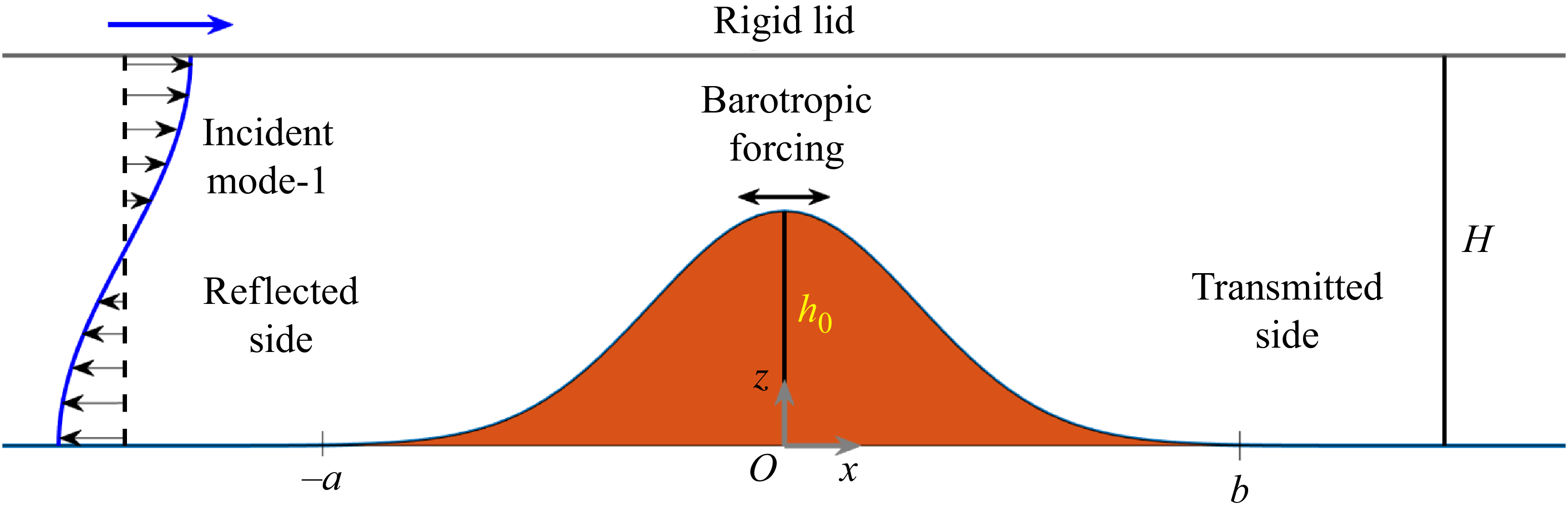
While modelling efforts usually treat generation and scattering as independent problems, in reality, they occur together. The extent of internal wave scattering may be affected by the presence of a barotropic tide and its interaction with the topography, and the extent of internal wave generation can be influenced by the presence of incident internal waves from elsewhere. Indeed, observations and numerical modelling have shown that when remotely generated internal waves interact with topography they can significantly alter the generation characteristics (Kelly & Nash Reference Kelly and Nash2010; Klymak et al. Reference Klymak, Buijsman, Legg and Pinkel2013). In the present study, the Green function approach is adapted to model the simultaneous generation and scattering of internal waves at an isolated ocean floor topography. This model is validated by numerical simulations. Figure 1 presents a schematic of the problem we study. A two-dimensional bottom topography of maximum height
 $h_0$
in an ocean of depth
 $H$
, experiences forcing from two different sources: (i) a barotropic forcing modelled as an oscillatory horizontal flow that is uniform throughout the depth, and (ii) a baroclinic left-to-right propagating incident mode-1 internal wave, assumed to be generated at a site far from the topography under consideration. The simultaneous presence of barotropic and baroclinic forcings results in a combined occurrence of internal wave generation and scattering.
A schematic showing a bottom topography of height
 $h_0$
in an ocean of depth
 $H$
, with a rigid lid representing the ocean surface. The forcing includes a barotropic oscillation and an incident baroclinic mode-1 internal wave, with a phase difference between the two (see 2.2).

The rest of the paper is organised as follows. The Green function formulation is discussed in § 2, followed by the simulation set-up in § 3. The results for an idealised isolated Gaussian topography in a uniform stratification are presented in § 4, followed by discussion and conclusions in § 5.
2. Theory
The Green function-based approach previously used to model topographic generation (Pétrélis et al. Reference Pétrélis, Smith and Young2006; Echeverri & Peacock Reference Echeverri and Peacock2010) and scattering (Mathur et al. Reference Mathur, Carter and Peacock2014) of internal waves is used in our two-dimensional study in the linear regime. This approach decomposes the streamfunction
 $\psi$
associated with the net flow field into
 \begin{equation} \psi (x,z,t) = \psi _b(x,z,t) + \psi '(x,z,t), \end{equation}
where
 $(x,z)$
are spatial Cartesian coordinates in a two-dimensional plane (see figure 1) and
 $t$
is time. The corresponding velocity field in the
 $(x,z)$
-plane is
 $(u,w) = (-\partial \psi /\partial z, \partial \psi /\partial x)$
. The streamfunctions associated with the background and perturbation flow fields are
 $\psi _b$
and
 $\psi '$
, respectively.
We consider a background flow composed of both barotropic and baroclinic components, both occurring at the same frequency
 $\omega$
. This allows us to write
 $\psi _b$
as
 $\psi _b(x,z,t) = {Re}[\phi _b(x,z)e^{-i\omega t}]$
, where
 $\phi _b(x,z)$
is a complex amplitude and
 $\textrm {Re}$
denotes the real part. In this study,
 $\phi _b$
includes the following contributions from a barotropic flow and a baroclinic mode-1 internal wave:
 \begin{equation} \phi _b(x,z) = -U_{0}z - \varPhi _1(z) \exp \left [i\left ( k_1 x+\varTheta \right )\right ], \end{equation}
where
 $U_0$
is the horizontal velocity amplitude of the barotropic forcing,
 $\varPhi _1(z)$
and
 $k_1$
are the vertical structure (mode shape) and horizontal wavenumber of the baroclinic mode-1 internal wave at frequency
 $\omega$
, respectively,
 $\varTheta$
is the phase difference between the barotropic and baroclinic components of the background flow and
 $\varPhi _1(z)$
corresponds to the horizontally propagating mode-1 over a flat bottom, and satisfies the boundary conditions
 $\varPhi _1(z=0) = \varPhi _1(z=H) = 0$
. Mode shapes are discussed more in detail after (2.4). We assume a linear regime, resulting from small excursion numbers, i.e. the horizontal fluid particle displacements associated with the background flow are significantly smaller than the horizontal length scales in the topography. While
 $\phi _b (x,z)$
is constant at
 $z=0,H$
, and hence satisfies the no-normal-flow boundary condition at the flat bottom and top, it is noteworthy that
 $\phi _b$
is not constant along the bottom topography
 $z = h(x)$
if
 $h(x)\ne 0$
. A constraint on the perturbation streamfunction
 $\psi '$
is therefore to ensure that the net flow field satisfies the no-normal-flow boundary condition on the topography.
We normalise
 $\varPhi _1(z)$
such that
 $\max |{{\rm d}\varPhi _1/{\rm d}z}| = 1$
, which results in
 $U_0$
representing a measure of the strength of the barotropic forcing relative to the strength of the mode-1 internal wave. The mode-1 internal wave in the background is assumed to be incident from the left of the topography under consideration (see figure 1). Large
 $U_0$
represents the generation-only limit, and
 $U_0 = 0$
is the scattering-only limit. In summary, for a given stratification, Coriolis frequency, internal wave frequency and ocean depth, the background flow associated with the simultaneous generation and scattering problem is characterised by two parameters:
 $ U_0$
and
 $\varTheta$
.
For small-amplitude perturbations, the streamfunction
 $\psi '$
associated with the perturbation flow field can be assumed to occur at the same frequency as the background flow, thus allowing us to write
 $\psi '(x,z,t)$
=
 $ {Re}[\phi ' (x,z)e^{-i\omega t}]$
, where
 $\phi '$
is the complex perturbation streamfunction amplitude. In the Green function approach,
 $\phi '$
is modelled as the sum of contributions from a distribution of sources (
 $\gamma (x')$
) placed on the topography
 \begin{equation} \phi '(x,z) = \int _{-a}^b \gamma (x') G(x,x';z,z')\, {\rm d}x', \end{equation}
where
 $-a \leqslant x'\leqslant b$
is the horizontal extent of the bottom topography, with a uniform ocean depth
 $H$
for
 $x'\lt -a$
and
 $x'\gt b$
. The Green function
 $G(x,x'; z,z')$
is (Mathur et al. Reference Mathur, Carter and Peacock2014)
 \begin{equation} G(x,x';z,z') = \sum _{n=1}^{\infty } \frac {\varPhi _n(z')}{2k_n} \left (\int _0^H \frac {N^2-\omega ^2}{\omega ^2-f^2}\varPhi _n^2(z) \, {\rm d}z \right )^{-1} e^{ik_n|{x-x'}|}\varPhi _n(z), \end{equation}
where
 $\varPhi _n(z)$
and
 $k_n$
are the vertical structure and the horizontal wavenumber of the streamfunction mode-
 $n$
, respectively, and
 $N(z)$
and
 $f$
are the stratification profile and background rotation strength, respectively. The mode shapes
 $\varPhi _n(z)$
, which satisfy the boundary conditions
 $\varPhi _n(z=0) = \varPhi _n(z=H) = 0$
, are normalised such that
 $max |{{\rm d}\varPhi _n/{\rm d}z}|\,=\,1$
. When the stratification is uniform
 $N(z) = N_0$
, the mode shapes and horizontal wavenumbers are given by
 $\varPhi _n(z) = [H/(n\pi )] \sin (n\pi z/H )$
and
 $k_n = n\pi /(H \cot \theta )$
, respectively, where
 $\cot ^2 \theta = (N_0^2-\omega ^2)/(\omega ^2-f^2)$
. For a non-uniform stratification
 $N(z)$
,
 $\varPhi _n(z)$
satisfies a Sturm–Liouville equation and
 $k_n$
is the corresponding eigenvalue, as discussed in Mathur et al. (Reference Mathur, Carter and Peacock2014).
The source strength distribution
 $\gamma (x')$
is chosen such that the net flow field satisfies the no-normal-flow boundary condition at the ocean floor, which can be written as
 \begin{equation} \phi '(x,z=h(x)) = -\phi _b(x,z=h(x)), \end{equation}
where
 $z = h(x)$
is the bottom topography such that
 $h(x) = 0$
for
 $x\lt -a$
and
 $x\gt b$
. It is noteworthy that
 $\phi '(x,z=H) = 0$
(2.3)–(2.4), thus satisfying the no-normal-flow boundary condition at the free surface modelled as a rigid lid. For a given
 $N(z),\, \omega ,\, f,\, h(x),\, U_0$
and
 $\varTheta ,\, \gamma (x')$
is obtained as the numerical solution of (2.5), as described in Echeverri & Peacock (Reference Echeverri and Peacock2010) and Mathur et al. (Reference Mathur, Carter and Peacock2014). It is worth noting that (2.3)–(2.5) represent a Fredholm integral equation of the first kind, with
 $\gamma (x')$
being the unknown function to solve for.
In the far field, where the ocean depth is constant, the net streamfunction amplitude
 $\phi = \phi _b + \phi '$
can be written as a summation of the barotropic forcing and a series of baroclinic internal wave modes
 \begin{equation} \phi (x,z) = -U_0z + \sum _{n=1}^{\infty } a^{\pm }_n \varPhi _n(z) e^{\pm ik_n x}, \end{equation}
where
 $a_n^{+}\, (a_n^{-})$
corresponds to left-to-right (right-to-left) propagating internal wave modal complex amplitudes in the
 $x\gt b\, (x\lt -a)$
region. Comparing (2.3) and (2.6), the modal amplitudes are obtained as
 \begin{equation} a_n^{\pm } = \frac {1}{2k_n} \!\left (\int _0^H{\kern-1pt} \frac {N^2-\omega ^2}{\omega ^2-f^2}\varPhi _n^2(z) \, {\rm d}z\! \right )^{-1} \!\!\!\int _{-a}^b \gamma (x') \varPhi _n(h(x')) e^{\mp ik_n x'} \, {\rm d}x' \text{ for } n\in \{1,2,3,{\cdots} \}. \end{equation}
Equation (2.7) is valid for all of the modal amplitudes except
 $a_1^+$
, for which the contribution from the background forcing has to be included. Specifically,
 $a_1^+$
is calculated as
 \begin{equation} a_1^{+} = -e^{i\varTheta }+ \frac {1}{2k_1} \left (\int _0^H \frac {N^2-\omega ^2}{\omega ^2-f^2}\varPhi _1^2(z) \, {\rm d}z \right )^{-1} \int _{-a}^b \gamma (x') \varPhi _1(h(x')) e^{- ik_1 x'} \, {\rm d}x', \end{equation}
where the first term comes from
 $\phi _b$
( 2.2).
In the far field, the depth-integrated time-averaged internal wave energy flux through a vertical section is related to the modal amplitudes via
 \begin{equation} E^{\pm } = \sum _{n=1}^{\infty } \left [\frac {\rho _0 (\omega ^2-f^2)}{2\omega }\int _0^H \left ( \frac {{\rm d}\varPhi _n}{{\rm d}z} \right )^2 \, {\rm d}z \right ]\frac {|{a_n^{\pm }|}^2}{k_n}, \end{equation}
where the superscripts
 $+$
and
 $-$
correspond to the left-to-right energy flux in the transmitted side
 $(x\gt b)$
and the right-to-left energy flux in the reflected side
 $(x\lt -a)$
, respectively. In the case of a uniform stratification, (2.9) simplifies to
 $E^{\pm }\,=\,\sum _{n=1}^{\infty } [\rho _0(\omega ^2-f^2)H^2\cot \theta /(4\pi \omega )]|{a_n^{\pm }|}^2/n$
. The total internal wave energy flux, including the scattered and the generated internal waves that radiate away from the topography, is
 $E^t = E^+ + E^-$
. In the absence of the incident mode-1 internal wave,
 $E^t$
reduces to the total internal wave energy flux generated by the barotropic forcing alone, and is denoted as
 $E^g$
. Conversely, in the limit of no barotropic forcing,
 $E^t$
is equal to
 $E^i$
, the incident mode-1 internal wave energy flux. When both incident mode-1 and barotropic forcing are present,
 $E^t$
is not necessarily equal to the sum
 $E^i + E^g$
. This departure from linear superposition of energy fluxes arises from constructive and destructive interferences between the generated and scattered wave fields. Remarkably,
 $E^t$
can even be smaller than
 $E^i$
, indicating that the presence of a barotropic forcing could irreversibly remove energy from the incident mode-1 internal wave.
To understand how
 $E^t$
can, and in many cases does, differ from
 $E^i+E^g$
, we first define two separate problems with their background flows given by
 $\phi _b^g = -z$
and
 $\phi _b^s = - \varPhi _1(z) \exp (ik_1 x)$
, respectively, such that
 $\phi _b$
in (2.2) can be written as
 $\phi _b = U_0\phi _b^g + \exp (i\varTheta )\phi _b^s$
. The perturbation streamfunction amplitudes corresponding to
 $\phi _b^g$
and
 $\phi _b^s$
are given by
 $\phi '^{,g}$
and
 $\phi '^{,s}$
, respectively. The perturbation streamfunction amplitude (and the corresponding modal amplitudes in the net flows fields) for the combined background flow in (2.2) can then be constructed as
 \begin{equation} (\phi ', a_n^{\pm }) = U_0 (\phi '^{,g}, a_n^{\pm , g})+ \exp (i\varTheta ) (\phi '^{,s}, a_n^{\pm , s}), \end{equation}
which would ensure that the boundary condition in (2.5) is satisfied. In (2.10),
 $a_n^{\pm ,g}$
and
 $a_n^{\pm ,s}$
are the complex modal amplitudes in
 $\phi ^g = \phi _b^g + \phi '^{,g}$
and
 $\phi ^s = \phi _b^s + \phi '^{,s}$
, respectively. It can be seen from (2.10) that the various modes from the individual generation and scattering problems could constructively or destructively interfere to form the net flow field in the combined problem. As a result, the energy fluxes in the individual modes, and hence the total internal wave energy flux, in the combined problem could be significantly smaller or larger than the sum of the energy fluxes in the individual problems.
As an example of destructive (constructive) interference, a mode-1 internal wave of unit amplitude can combine with another mode-1 of (1/10)th the amplitude to result in a minimum (maximum) mode-1 amplitude of 0.9 (1.1). In terms of energy fluxes, the destructive and constructive interferences result in a mode-1 of 81 % and 121 % of the unit amplitude mode-1, while the weaker mode-1 that was added contained only 1 % of the unit amplitude mode-1 energy flux. Therefore, a barotropic forcing which is capable of generating just 1 % of the incident mode-1 energy flux when acting alone, can either take away 19 % or generate an additional 20 % of the incident mode-1 energy flux. In the real problem, such interferences can occur over a distribution of modes.
To quantify the extent to which the internal wave energy fluxes in the combined forcing scenario are different from a summation of the energy fluxes in the individual scattering and the generation scenarios, we define
 \begin{equation} \eta = \frac {E^t}{E^g + E^i}. \end{equation}
Here,
 $\eta \gt 1$
(
 $\eta \lt 1$
) can be interpreted as stronger (weaker) topographic generation of internal waves in the combined forcing scenario when compared with the case of no incident mode-1.
3. Methods
3.1. Simulations
To validate the results of the Green function model, we simulate the internal wave field with the two-dimensional, non-dimensionalised Navier–Stokes equations in an inertial frame (
 $f=0$
), using the Boussinesq approximation for an inhomogeneous, incompressible fluid subject to gravity along the vertical direction
 $z$
. The Boussinesq approximation neglects the effects of density variation except in the buoyancy term, and is appropriate for buoyancy-driven flows with weak relative density variations around a reference value
 $\rho _{00}$
. The Navier–Stokes equations are non-dimensionalised with the reference density,
 $\hat {\rho }_{00} = 1000 \, \text{ kg}\,\rm m^{-3}$
, the height of the domain
 $\hat {H}=3800 \, \text{m}$
and the tidal frequency
 $\hat {\omega } = 1.4053 \times 10^{-4} \;\text{rad}\, \rm s^{-1}$
. The system of equations is
 \begin{align} \boldsymbol{\nabla }\boldsymbol{\cdot }\boldsymbol{u} &= 0,\end{align}
 \begin{align} \frac {\partial u}{\partial t} + (\boldsymbol{u} \boldsymbol{\cdot }\boldsymbol{\nabla }) u &= -\frac {\partial p}{\partial x} + \nu {\nabla} ^2 u,\end{align}
 \begin{align} \frac {\partial w}{\partial t} + (\boldsymbol{u} \boldsymbol{\cdot }\boldsymbol{\nabla }) w &= -\frac {\partial p}{\partial z} + \nu {\nabla} ^2 w - \rho g,\end{align}
 \begin{align} \frac {\partial \rho }{\partial t} + (\boldsymbol{u} \boldsymbol{\cdot }\boldsymbol{\nabla }) \rho & = \kappa {\nabla} ^2\rho ,\end{align}
where
 $\boldsymbol{u} = (u,w)$
is the dimensionless velocity field,
 $p$
is the dimensionless pressure and
 $\rho$
is the dimensionless local density. To balance numerical stability demands while minimising energy losses due to viscosity, the dimensionless viscosity
 $\nu = \nu ^*/\hat {H}^2 \hat {\omega }$
was based on a value of
 $\nu ^*$
that is 20 times that of water (
 $\nu _{w\textit{ater}}=10^{-6} \, \rm {m^2}\,\rm s^{-1}$
). To minimise the impact of diffusion, the dimensionless diffusivity is
 $\kappa =\kappa _{w\textit{ater}}/\hat {H}^2\hat {\omega }$
, where
 $\kappa _{w\textit{ater}} = 1.4\times 10^{-7}\,\rm {m^2}\,\rm s^{-1}$
is the thermal diffusivity for sea water (Kunze Reference Kunze2003). Finally, the dimensionless gravity is
 $g=\hat {g}/\hat {H}\hat {\omega }^2$
where
 $\hat {g} = 9.8 \, \rm {m}\,\rm s^{-2}$
is the gravity acceleration. To ensure that nonlinear effects are negligible, the forcings in (2.2) are multiplied by a factor of 0.1 in the numerical simulations.
The system of (3.1)–(3.4) is solved numerically for
 $u$
,
 $w$
,
 $p$
and
 $\rho$
using CDP 2.4, an unstructured, finite-volume based, large eddy simulation code that implements a fractional-step time-marching scheme (Ham & Iaccarino Reference Ham and Iaccarino2004; Mahesh, Constantinescu & Moin Reference Mahesh, Constantinescu and Moin2004). All subgrid-scale modellings are turned off, and the code is modified to include the buoyancy term in (3.3) and to solve (3.4) along with (3.1)–(3.3). This code has previously been used to simulate internal waves in various settings and has been validated with experiments (King, Zhang & Swinney Reference King, Zhang and Swinney2009; Dettner, Paoletti & Swinney Reference Dettner, Paoletti and Swinney2013; Lee et al. Reference Lee, Paoletti, Swinney and Morrison2014; Paoletti, Drake & Swinney Reference Paoletti, Drake and Swinney2014; Zhang & Swinney Reference Zhang and Swinney2014; Allshouse et al. Reference Allshouse, Lee, Morrison and Swinney2016; Vieira & Allshouse Reference Vieira and Allshouse2020).
The simulations were conducted over a spatial domain spanning from −750 to 1000 in the
 $x$
-direction and 0 to 1 in the
 $y$
-direction. The mesh resolution consisted of 46 667 grid points in the
 $x$
-direction and 401 grid points in the
 $y$
-direction, ensuring sufficient resolution to capture the key features of the internal wave dynamics. The computational domain was periodic in the
 $x$
-direction, and free-slip, insulating and no-flux boundary conditions were applied at the top and bottom boundaries. A time step of 5000 steps per wave period was found to be sufficiently small to achieve converged results. To confirm that start-up effects had dissipated, the system was run for 25 periods to ensure that time-periodic behaviour had been fully established. Both spatial and temporal properties were systematically varied in the study to assess their influence on the simulation results with results demonstrating less than 1 % variation.
In our numerical simulations, we use sponge layers in two distinct regions of the domain to generate both barotropic and baroclinic internal waves. The sponge layers nudge the velocity toward a prescribed target field
 $\boldsymbol{u}_{\textit{tar}}(\boldsymbol{x},t)$
. This is acheived by including a forcing term,
 $-\,M(\boldsymbol{x}) (\boldsymbol{u}-\boldsymbol{u}_{\textit{tar}} )/\tau$
, where
 $M(\boldsymbol{x})$
is a mask that ramps up smoothly from 0 to 1 using a
 $\tanh$
profile to minimise reflections;
 $\tau$
and the
 $\tanh$
ramp thickness are tuned to balance accurate wave generation and effective absorption with minimal reflection. The first damping region, spanning from
 $x = 250$
to
 $x = 950$
, serves a dual purpose: it dampens the scattered wave field, preventing its transmission through the periodic boundary, and simultaneously generates the tidal flow. The second damping region, located between
 $x = -550$
and
 $x = -250$
, is used to attenuate any reflected waves off the topography while facilitating the generation of both barotropic and baroclinic forcing. To prevent unwanted reflections of energy off these damping regions, the strength of the Rayleigh damping is smoothly varied across the entire domain. This strategy ensures the controlled development of the internal wave dynamics, effectively supporting the study of wave–topography interactions and energy propagation without introducing spurious effects. Forcing parameters were tuned in an identical domain without a topography to ensure that the desired wave field was being produced.
3.2. Modal decomposition analysis
For a quantitative comparison between theory and simulations, we perform a modal decomposition of the simulation data. The net horizontal velocity fields in the transmitted (
 $x\gt b$
) and reflected (
 $x\lt -a$
) regions are written, respectively, as
 \begin{align} u_t(x,z,t)& = \textrm {Re}\left [U_0e^{-i\omega t}+\sum _{n=1}^{\infty }a_{n,t}^{+}\cos \left (\frac {n\pi z}{H} \right )e^{i(k_nx-\omega t)}\right ]\!,\end{align}
 \begin{align} u_r(x,z,t)& = \textrm {Re}\left [ U_0e^{-i\omega t}+\sum _{n=1}^{\infty }a_{n,r}^{\pm }\cos \left (\frac {n\pi z}{H} \right )e^{i(\pm k_nx-\omega t)}\right ]\!,\end{align}
where the subscripts
 $t$
and
 $r$
refer to the transmitted and reflected regions, and the superscripts
 $+$
and
 $-$
refer to left-to-right and right-to-left propagating waves. The complex amplitudes
 $a_{n,t}^+$
and
 $a_{n,r}^{\pm }$
contain information about both the amplitude and phase of mode
 $-n$
. In the reflected region, it is expected that the left-to-right propagating waves are comprised of the incident mode-1 only, i.e.
 $a_{1,r}^+ = \exp (i\varTheta )$
and
 $a_{n,r}^+ = 0$
for
 $n\gt 1$
.
Modal decomposition is performed after the simulation velocity field attains a time-periodic state i.e. after 25 periods. On the transmitted side, a location
 $x = x_0(\gt b )$
close to the topography is chosen, and the Fourier amplitude and phase of
 $u$
at the forcing frequency
 $\omega$
is estimated at every depth. The magnitude of the modal amplitudes is then calculated as
 \begin{align} |{a_{n,t}^+}| = \frac {2}{H} \sqrt {\left (\int _0^H \tilde {u}_t(x_0,z,t_1)\cos \left (\frac {n\pi z}{H} \right )\, {\rm d}z\right )^2+\left (\int _0^H \tilde {u}_t(x_0,z,t_2)\cos \left (\frac {n\pi z}{H} \right )\, {\rm d}z\right )^2 }, \end{align}
where
 $\tilde {u}_t$
is the filtered horizontal velocity at
 $\omega$
. The times
 $t_1$
and
 $t_2$
are chosen such that
 $\omega (t_2-t_1) = \pi /2$
. On the reflected side, the number of modal amplitudes is twice that of the transmitted side owing to the presence of right-to-left propagating waves too. As a result, simulation data from two different horizontal locations are used to calculate
 $a_{n,r}^{\pm }$
using expressions (Appendix A) that build on the same idea as in (3.7). To minimise the influence of viscous effects in the comparison between simulations and theory, we choose
 $x_0 (\gt b$
or
 $\lt -a)$
to be as close to the topography as possible.
4. Results
In this section, we consider the case of an isolated Gaussian topography:
 $h(x) = h_0\exp (-x^2/\sigma ^2)$
in a uniformly stratified ocean (
 $N(z) = N_0$
, a constant) with no background rotation (
 $f = 0$
). The ends of the topography are chosen to be at
 $x = -2.7\sigma$
and
 $x = +2.7\sigma$
. Two non-dimensional parameters characterise the Gaussian topography: height ratio
 $h^* = h_0/H$
(see figure 1 for definition of
 $h_0$
and
 $H$
) and criticality
 $\epsilon = \textit{max} (|{\rm d}h/{\rm d}x|)/\tan \theta$
, where
 $\tan \theta = \omega /\sqrt {N_0^2-\omega ^2}$
is the internal wave ray slope. For the theoretical calculations (Green function-based approach), the Gaussian topography is represented using 2161 horizontally equispaced points, and the Green function in (2.4) is calculated as a summation from
 $n = 1$
to
 $n = 2161$
. For the numerical simulations, the following representative values are chosen for the various parameters:
 $\omega = 1.4053\times 10^{-4}\, \text{rad}\, \text{s}^{-1}$
,
 $N_0^2 = 3\times 10^{-5}$
rad
 $^2$
s
 $^{-2}$
and
 $H = 3800$
m.
4.1. Wave fields
To provide some baseline intuition about the generation, scattering and combined wave fields, we first present representative snapshots of the horizontal velocity field (excluding the barotropic component). Figures 2 and 3 correspond to topographic parameter values of
 $(h^*,\epsilon ) = (0.3,0.3)$
and
 $(0.3,2.0)$
, respectively. The barotropic forcing amplitudes (see (2.2)) in figures 2 and 3 are
 $U_0 = 2.79$
and 0.45, respectively. These values of
 $U_0$
correspond to
 $E^g/E^i = 0.49$
and 0.17, respectively, and result in significant sensitivity to
 $\varTheta$
as shown later in figure 8. The theoretical horizontal velocity fields presented in this section were constructed using the first 300 modes of the solution.
Snapshots of horizontal velocity (without the barotropic component) for (a) generation only, (b) scattering only and (c), (d) combined generation and scattering and
 $\varTheta = \pi /6$
,
 $7\pi /6$
, respectively. Panels (a)–(d) are based on Green function theory; (e)–(f) are the same as (c)–(d), but based on numerical simulations. All the snapshots, taken from
 $t = 0$
, correspond to
 $(h^*,\epsilon ) = (0.3,0.3)$
and
 $U_0 = 2.79$
.

Snapshots of horizontal velocity (without the barotropic component) for (a) generation only, (b) scattering only and (c), (d) combined generation and scattering and
 $\varTheta = \pi /6$
,
 $7\pi /6$
, respectively. Panels (a)–(d) are based on Green function theory; (e)–(f) are same as (c)–(d), but based on numerical simulations. All the figures correspond to
 $(h^*,\epsilon ) = (0.3,2.0)$
and
 $U_0 = 0.45$
. Snapshots in (c) and (e) are at
 $\omega t = \pi /6$
, while the snapshots in (d) and (f) are at
 $\omega t\,=\,7\pi /6$
.

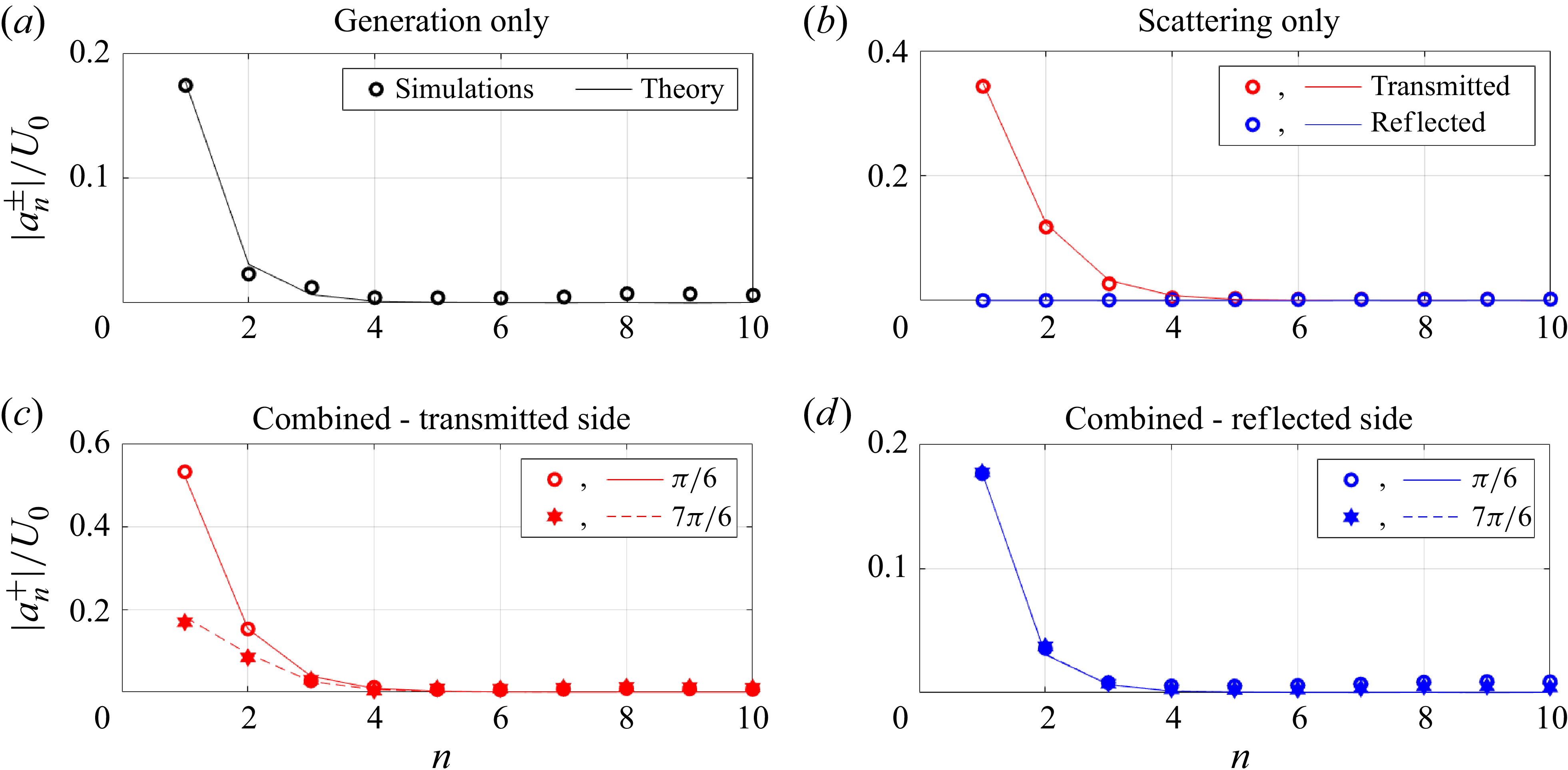
Figures 2(a) and 2(b) show the snapshots from the individual generation and scattering problems, i.e. in the absence of incident baroclinic mode-1 and barotropic forcing, respectively. Figure 2(a) shows the generation of internal waves of equal strength to the left and the right, which is owing to the topography’s symmetry. While mode-1 seems to be dominant, the spatial structure indicates the presence of higher modes too. Figure 2(b) shows that the incident internal wave energy gets mostly transmitted in the absence of barotropic forcing, which is consistent with earlier studies demonstrating minimal reflection in the case of subcritical topography (Müller & Liu 2000; Johnston & Merrifield Reference Johnston and Merrifield2003; Mathur et al. Reference Mathur, Carter and Peacock2014). In addition, the spatial structure of the wave field on the transmitted side indicates the transfer of energy from incident mode-1 to higher modes, which is quantified in figure 4.
Distribution of horizontal velocity modal amplitudes (normalised with respect to
 $U_0$
) from theory (solid and dashed lines) and simulations (symbols) for the case of
 $(h^*,\epsilon ) = (0.3,0.3)$
and
 $U_0 = 2.79$
, with the top row showing results from (a) barotropic forcing (generation) only and (b) baroclinic forcing (scattering) only. In the bottom row, results from the combined forcing case are shown for two different phase differences
 $\varTheta = \pi /6$
and
 $7\pi /6$
, with (c) and (d) corresponding to transmitted and reflected sides, respectively. Note that the range of values on the
 $|a_n^{\pm }|/U_0$
-axis is different in panels (a)–(d).

Figures 2(c) and 2(d) present the snapshots of the wave fields in the combined forcing problem for two phase differences:
 $\varTheta = {\pi /6}$
and
 $7\pi /6$
, respectively. The time instant in both figures is
 $t = 0$
, in phase with the barotropic forcing. As shown by (2.10), the wave fields in the combined problem can be constructed as a linear superposition of the wave fields in the individual generation and scattering problems shown in figures 2(a) and 2(b). Compared with the generation-only wave field in figure 2(a), the combined forcing wave fields in figure 2(c–d) seem to contain finer spatial scales in the internal wave beams, suggesting a stronger presence of
 $n\gt 1$
modes. Furthermore, in contrast to the scattering-only wave field, reflected waves are more noticeable in the combined forcing scenarios. For the combined forcing problem, there are noticeable differences in the wave fields between
 $\varTheta = {\pi /6}$
and
 $\varTheta = {7\pi /6}$
(both are plotted at
 $t = 0$
), although it is difficult to ascertain differences in the individual mode strengths just based on these plots in figure 2(c–d). Finally, snapshots from numerical simulations (figure 2
e–f) show excellent qualitative and quantitative agreement with theory, thus providing some validity to the theory.
Similar to figure 2, figure 3 shows horizontal velocity snapshots, but for the supercritical case of
 $(h^*,\epsilon ) = (0.3,2.0)$
. As mentioned earlier, the wave fields in figure 3 are plotted for
 $U_0 = 0.45$
, which corresponds to
 $E^g/E^i = 0.17$
. In the individual generation and scattering problems, significantly finer-scale wave beam features are observed, consistent with previous generation (Echeverri et al. Reference Echeverri, Flynn, Winters and Peacock2009) and scattering (Mathur et al. Reference Mathur, Carter and Peacock2014) studies on supercritical topography. Such sharp changes or discontinuities are singular features that can be traced back to similar features in the Green function in the linear, inviscid limit. These fine-scale wave beam features are indicative of the presence of high modes, which are quantified in figure 5. While the scattering-only problem showed complete transmission of the incident mode-1 for the subcritical topography (figure 2
b), scattering by supercritical topography shows significant reflection too (figure 3
b).
Same as figure 4, but for
 $(h^*,\epsilon ) = (0.3,2.0)$
and
 $U_0 = 0.45$
. Note that the range of values on the
 $|a_n^{\pm }|/U_0$
-axis is different in panels (a)–(d).

Figures 3(c) and 3(d) show snapshots of the wavefield for the combined forcing problem for
 $\varTheta = \pi /6$
and
 $\varTheta = 7\pi /6$
, respectively. Unlike in figure 2, the time instants in figure 3 are chosen to be in phase with the incident mode-1, given that
 $E^i$
dominates
 $E^g$
for
 $(h^*,\epsilon ) = (0.3,2.0)$
and
 $U_0 = 0.45$
. The wave fields in the combined forcing scenarios show relatively stronger similarity with the scattering-only wave field when compared with the subcritical case presented in figure 2. This can be understood to be a consequence of the relatively smaller value of
 $E^g/E^i$
, which suggests that the combined forcing problem may be dominated by the scattering-only problem. The snapshot from numerical simulations for
 $\varTheta = \pi /6$
shows overall qualitative agreement with the theory, albeit with much weaker velocities and smoother features. These differences are likely due to viscous effects in the simulations, which act strongly on higher modes. The simulation (figure 3
e) also shows weak higher frequency features (steeper than the wave beams at the forcing frequency), which are beyond the scope of linear theory and the current study. For
 $\varTheta = 7\pi /6$
, regions of negative horizontal velocity are similar between theory and simulations (figures 3
d and 3
f), whereas the positive horizontal velocity regions in theory show up with noticeably weak velocities in the simulations. The exact phase associated with these snapshots may influence this difference, and we proceed to compare the wave field amplitudes.
In addition to the wave field snapshots in figures 2 and 3, we also compared the wave field amplitudes between theory and simulations, as shown in figures 14–15 in Appendix B. The subcritical case (figure 14) shows that the theory and simulations are in excellent agreement in highlighting the difference between
 $\varTheta = \pi /6$
and
 $\varTheta = 7\pi /6$
. The theory and simulations show good agreement for the supercritical case (figure 15) too, but with the simulations under-predicting the amplitudes along the wave beams due to viscous effects. In summary, the wave field snapshots and amplitudes show reasonable qualitative and quantitative agreement between theory and simulations for the subcritical case, and excellent qualitative agreement for the supercritical case. As discussed in the later sections, the lack of quantitative agreement for the wave fields in the supercritical case does not necessarily imply large differences in the modal amplitudes and energy fluxes.
4.2. Validation
We proceed to present a quantitative validation of the theory by comparing the theoretical individual mode strengths with those from simulations. In the process (figures 4–6), we also begin to see the dependence of the net wave field and its modal distribution on the topographic and forcing parameters.
Same as figure 4, but for
 $(h^*,\epsilon ) = (0.6,2.0)$
and
 $U_0 = 0.30$
. Note that the range of values on the
 $|a_n^{\pm }|/U_0$
-axis is different in panels (a)–(d).

Figure 4 shows the distribution of the horizontal velocity modal amplitudes (normalised by
 $U_0$
) for the case of a short, subcritical topography characterised by
 $(h^*,\epsilon ) = (0.3,0.3)$
and a forcing specified by
 $U_0 = 2.79$
. In the absence of the incident mode-1 internal wave, generation due to barotropic forcing results in a predominantly mode-1 internal wave field (figure 4
a), with 98.4 % of the total internal wave energy flux present in mode-1. When there is no barotropic forcing, nearly all the incident mode-1 internal wave energy gets transmitted, with 93.9 % of the incident energy still in mode-1 in the transmitted wave field (figure 4
b). As noted in § 4.1,
 $U_0 = 2.79$
corresponds to
 $E^g/E^i = 0.49$
here.
When the barotropic and baroclinic forcings are combined, the comparable mode-1 amplitudes observed in the generation-only and scattering-only problems can constructively or destructively interfere in the transmitted side based on the value of
 $\varTheta$
. Indeed, the mode-1 amplitude in the transmitted side (figure 4
c) is close to the sum of the amplitudes in figures 4(a) and 4(b) for
 $\varTheta = \pi /6$
. For
 $\varTheta = 7\pi /6$
, the amplitude is approximately the difference between the amplitudes in figures 4(a) and 4(b). This has significant implications for the total internal wave energy in the two cases, as presented later in figure 7.
Variation of
 $\eta = E^t/(E^i+E^g)$
with the phase difference
 $\varTheta$
for
 $(h^*,\epsilon ) =$
(a)
 $(0.3,0.3)$
, (b)
 $(0.3,2.0)$
and (c)
 $(0.6,2.0)$
. The values of
 $U_0$
and
 $E^g/E^i$
are indicated within each panel. Solid lines and symbols correspond to theory and simulations, respectively. Panels (d–f) show the variation of
 $\eta ^g = (E^t-E^i)/E^g$
and
 $\eta ^l = (E^i-E^t)/E^i$
with
 $\varTheta$
for the same cases as in (a–c), respectively. The blue and red portions correspond to when
 $E^t\gt E^i$
and
 $E^t\lt E^i$
, respectively.

Such interference is observed for mode-2 as well on the transmitted side, resulting in notably different amplitudes for
 $\varTheta = \pi /6$
and
 $7\pi /6$
in figure 4(c). On the reflected side, however, the wave field radiating away from the topography in the combined forcing problem is nearly identical to the corresponding wave field in the generation-only problem regardless of phase; we recall from figure 4(b) that the subcritical topography under consideration reflects a negligible fraction of the incident mode-1 in the scattering only problem. Finally, figure 4 also reveals good quantitative agreement between theory (lines in figure 4) and simulations (markers in figure 4) for the mode strength distributions in both the transmitted and reflected sides.
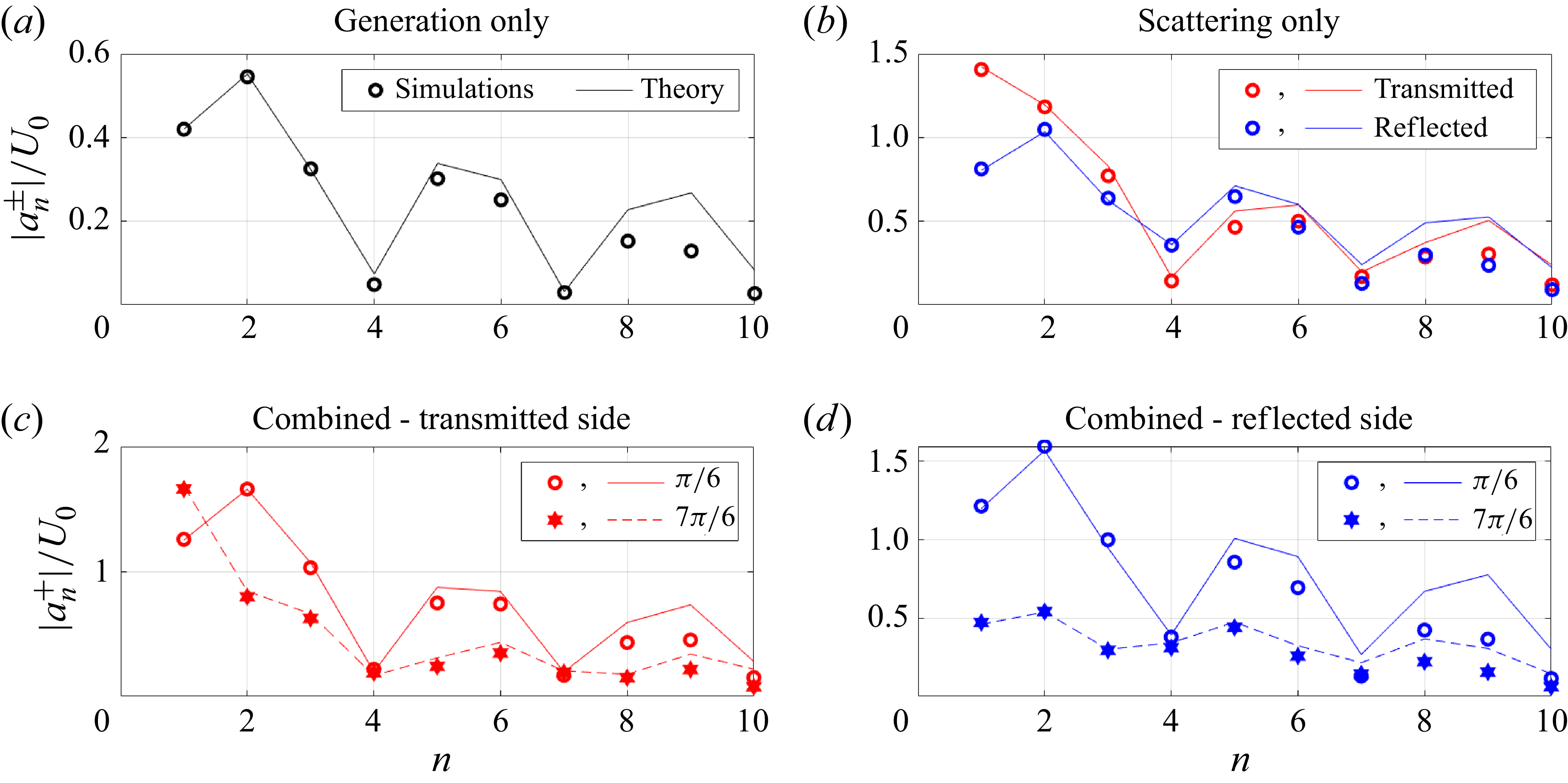
Figure 5 presents the case of a short, supercritical topography characterised by
 $(h^*,\epsilon )\,=\,(0.3,2.0)$
and a forcing specified by
 $U_0 = 0.45$
. In contrast to the subcritical topography of the same height ratio presented in figure 3(a), barotropic forcing alone generates internal waves at multiple higher modes, with mode-1 accounting only for 42.23 % of the total generated internal wave energy (figure 5
a). Similarly, in the scattering-only scenario, the energy from incident mode-1 gets redistributed to multiple higher modes, with a significant fraction (31.73 %) of the incident energy getting reflected too (figure 5
b). As a result, in the combined forcing scenario, the phase difference between the barotropic and incident mode-1 forcings can significantly influence the wave fields in both the transmitted and reflected sides. Indeed, as observed in figures 5(c)–5(d), there are significant differences between
 $\varTheta$
=
 $\pi /6$
and
 $7\pi /6$
for most of modes 1–10 on the transmitted and reflected sides. For example, modes 2 and 1 are dominant (in terms of amplitude) in the wave field on the transmitted side for
 $\varTheta = \pi /6$
and
 $7\pi /6$
, respectively (figure 5
c). On the reflected side, there is noticeable difference between
 $\varTheta = \pi /6$
and
 $7\pi /6$
for both mode-1 and mode-2 amplitudes (figure 5
d).
In terms of the energy ratio,
 $U_0 = 0.45$
corresponds to
 $E^g/E^i = 0.17$
, suggesting that generation by barotropic forcing is relatively weak. While this may indicate that the combined forcing scenario would be similar to the scattering-only scenario, figures 5(c) and 5(d) highlight that the interference between the various modes can significantly modify the net wave field depending on the phase difference in the forcings. Finally, as we observed in figure 4, there is a good quantitative agreement between theory and simulations in figure 5 too, albeit with some differences observed for modes 5 and higher. These differences at higher modes are likely due to viscous effects in the simulations.
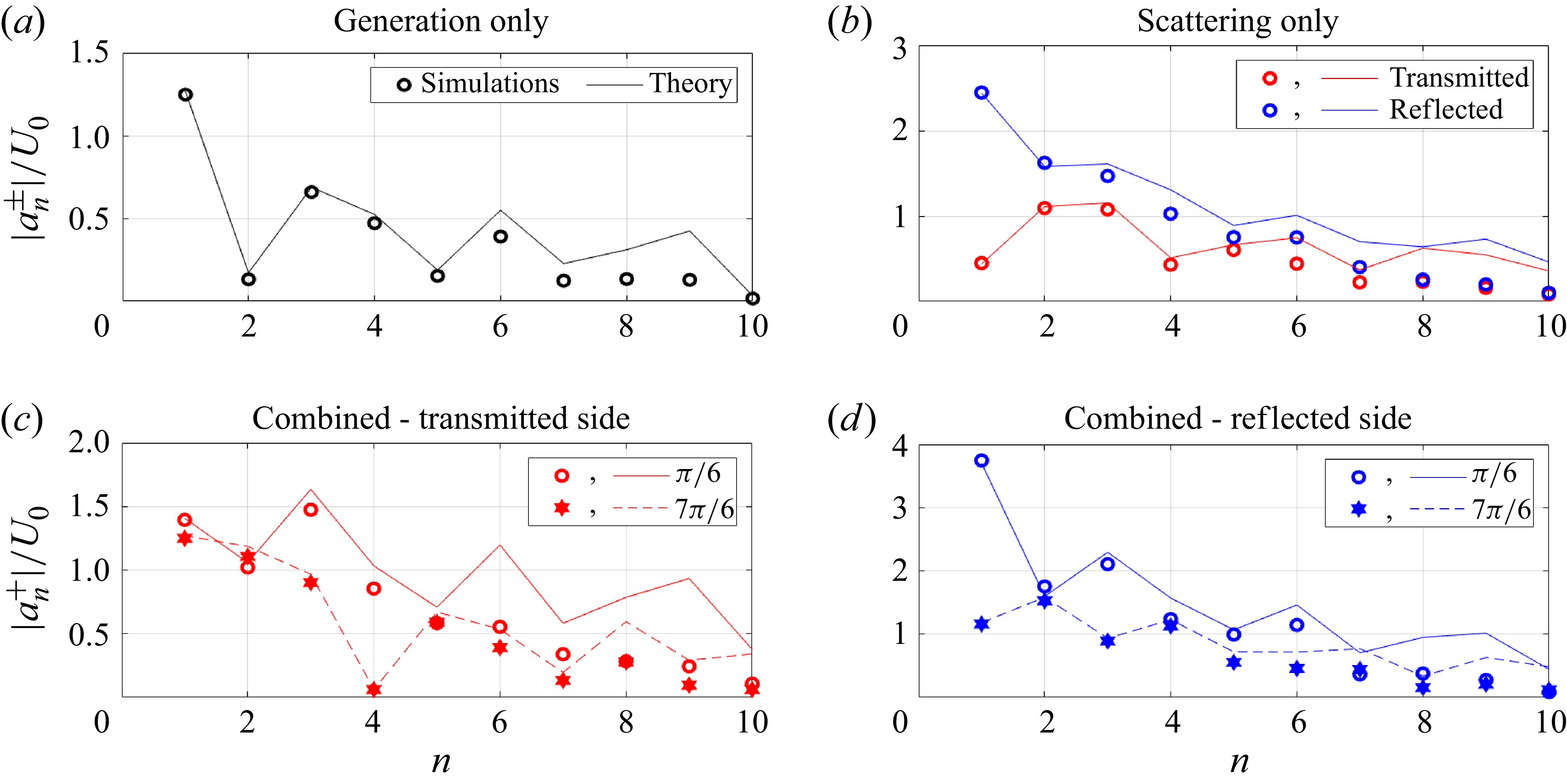
Figure 6 shows the results for a tall, supercritical topography,
 $(h^*,\epsilon ) = (0.6,2.0)$
, and a relative barotropic forcing amplitude of
 $U_0 = 0.30$
. The internal wave field generated by the barotropic forcing alone is dominated by mode-1, has a relatively small amplitude for mode-2, and non-negligible amplitudes for modes 3 and higher (figure 6
a). In the scattering-only scenario, a significant fraction (80.71 %) of the incident mode-1 energy is reflected, while appreciable scattering to higher modes is also observed (figure 6
b). In the combined forcing scenario, modes 1 and 2 on the transmitted side essentially mimic their corresponding strengths in the generation-only and scattering-only scenarios, respectively (figure 6
c). For modes 3 and 4, however, owing to appreciable contributions from both the generation-only and scattering-only cases, there is a noticeable difference between
 $\varTheta = \pi /6$
and
 $7\pi /6$
(figure 6
c). On the reflected side in the combined forcing scenario, mode-1 amplitudes are drastically different for
 $\varTheta = \pi /6$
and
 $7\pi /6$
because of constructive and destructive interference, respectively (figure 6
d). Finally, as observed in figures 4 and 5, there is excellent quantitative agreement between theory and simulations at low modes (up to mode-5), and somewhat reasonable agreement at higher modes.
In summary, figures 4–6 highlight how the internal wave field in the combined forcing scenario can be sensitively dependent on the phase difference between the barotropic forcing and the incident baroclinic mode-1.
4.3. Effects of phase difference on energetics
In addition to the influence of the phase difference on the individual mode strengths in the internal wave field, it is of interest to investigate whether the total energy in the internal wave field is dependent on
 $\varTheta$
. As defined in (2.11),
 $\eta = E^t/(E^i+E^g)$
quantifies the total internal wave energy flux (transmitted and reflected sides) in the combined forcing problem, normalised by the sum of the energy fluxes in the generation-only and scattering-only scenarios.
Figure 7(a)–(c) shows the variation of
 $\eta$
with
 $\varTheta$
for the same three topographies and forcing amplitudes considered in figures 4–6. For the sake of comparison between theory and simulations,
 $\eta$
is calculated based on modes 1–10 in figure 7. Interestingly,
 $\eta$
shows significant deviations from unity in all three cases. The mean value of
 $\eta$
is 1; i.e. when averaged across all values of
 $\varTheta$
, the total internal wave energy flux radiating away from the topography in the combined forcing scenario equals the sum of the energy flux generated by the barotropic forcing alone and the energy flux of the incident baroclinic mode-1. For
 $(h^*,\epsilon ) = (0.3,0.3)$
and
 $E^g/E^i = 0.49$
, the maximum and minimum values of
 $\eta$
are 1.66 and 0.34, respectively, occurring near
 $\varTheta = \pi /4$
and
 $3\pi /4$
(figure 7
a). This represents a 66 % increase or decrease from the average value, thus establishing that the total internal wave energy flux can vary significantly with
 $\varTheta$
. Corresponding maximum deviations from
 $\eta = 1$
are 32 % and 57 % in figures 7(b) and 7(c), respectively.
It is also possible to define
 \begin{equation} \eta ^g = \frac {E^t-E^i}{E^g}, \end{equation}
whose deviation from unity is a measure of the extent to which the incident baroclinic mode-1 affects internal wave generation by the barotropic tide. Interestingly,
 $\eta ^g\lt 0$
occurs for some values of
 $\varTheta$
i.e. the energy flux radiating away from the topography is less than that of the energy flux of the incident mode-1 internal wave. In such scenarios, we define
 \begin{equation} \eta ^l = \frac {E^i-E^t}{E^i}, \end{equation}
as a measure of the fraction of the incident mode-1 energy flux that is lost to some other form in the presence of the barotropic tide. This `other form’ could be associated with energy being put back into barotropic tides or dissipative work over the topography or other nonlinear effects, none of which are represented in the current theory. As shown in Appendix C, while the sources represent a forcing or work done at their locations, it is not possible to directly evaluate it in the current framework.
Figure 7(d–f) shows the variation of
 $\eta ^g \text{ and } \eta ^l$
with
 $\varTheta$
when
 $E^t\gt E^i$
and
 $E^t\,\lt \,E^i$
, respectively. In each of figure 7(d–f),
 $ \eta ^g\gt 1$
occurs for half the range of
 $\varTheta$
, indicating stronger internal wave generation in the presence of the incident mode-1. Interestingly, the maximum
 $\eta ^g$
in all the three cases corresponds to internal wave generation in the combined forcing scenario being nearly three times as energetic as that with barotropic forcing alone. In the remaining range of
 $\varTheta$
where
 $\eta ^g\lt 1$
, small values of
 $\eta ^g$
indicate significantly weaker internal wave generation in the combined forcing scenario. Remarkably, for a significant range (
 $\gt \pi /2$
in extent) of
 $\varTheta$
,
 $\eta ^g \lt 0$
occurs, which corresponds to a fraction of the incident mode-1 energy flux being lost to another form. Quantifying this energy loss in terms of
 $\eta ^l$
, up to around 49.2 %, 21.1 % and 41.8 % of the incident mode-1 energy flux is lost to other processes over the topography as presented in figure 7(d–f), respectively.
In summary, while the average behaviour in the combined forcing scenario can be described by the internal wave energy flux radiating away from the topography being equal to
 $E^g + E^i$
, there can be significant deviations from the average based on the phase difference between the barotropic and baroclinic forcings. For half the range of
 $\varTheta$
, the effective internal wave generation is enhanced by the incident mode-1. In the other half of the range of
 $\varTheta$
, internal wave generation is either significantly suppressed or not present at all. In the latter scenario of internal wave generation being completely suppressed, the barotropic forcing even serves to transfer a significant fraction of the incident mode-1 energy to other processes in the region of the topography. Fine-scale numerical simulations that accurately resolve the flow fields in the vicinity of the topography, along with a detailed energy budget analysis, are required to further understand the mechanism by which energy from the incident mode-1 is converted into other forms over the topography when a barotropic forcing is also present.
Finally, figure 7(a–c) also reveals good quantitative agreement between theory and simulations for the derived quantity
 $\eta$
, which is consistent with the quantitative agreement already reported for the individual low-mode amplitudes in figures 4–6. The discrepancies between theory and simulations for high-mode
 $(n\geqslant 5)$
amplitudes in the supercritical cases (figures 6–7) do not significantly affect the overall energy fluxes. It is noteworthy that energy fluxes in individual modes go as
 $\sim |{a_n^{\pm }|}^2/n$
(2.9), as a result of which low modes still dominate the overall energetics. For example, for
 $(h^*,\epsilon ) = (0.6,2.0)$
,
 $U_0 = 0.30$
and
 $\varTheta = \pi /6$
, the values of
 $\eta$
obtained from theory using the first 4 and 10 modes are 1.40 and 1.50, respectively, whereas for the simulations, they are 1.38 and 1.45, respectively. Corresponding values for
 $\varTheta = 7\pi /6$
are 0.39 and 0.43 from theory, and 0.37 and 0.39 from simulations.
These comparisons between theory and simulations for three different topographies at forcing amplitudes where there is a strong dependence of the internal wave field on
 $\varTheta$
serve to validate the theory in the linear internal wave regime with combined forcing. We proceed to present detailed theoretical results over a large sweep of the different parameters, including
 $\varTheta$
,
 $U_0$
,
 $h^*$
and
 $\epsilon$
, to address various questions. For example, does
 $\eta$
deviate significantly from unity even when the barotropic forcing or the incident baroclinic mode-1 is relatively weak? In other words, to what extent can a weak barotropic forcing modify the topographic scattering of an incident mode-1 internal wave? Similarly, can a weak incident baroclinic mode-1 significantly influence the internal wave generation by barotropic forcing? Another related question of interest is the parameter regime over which the presence of barotropic forcing can actually result in the loss of the incident mode-1 internal wave energy to some other form, as quantified by
 $\eta ^l$
.
4.4. Total energy flux
Figure 8 shows the variation of
 $\eta$
with
 $\varTheta$
and
 $E^g/E^i$
for four different topographies, three of which were considered in figures 4–7. For a given topography, the individual generation and scattering problems are solved first, following which (2.10) is used to construct the wave fields for different combinations of
 $U_0$
and
 $\varTheta$
. To examine the limits of a weak barotropic forcing and a weak incident baroclinic mode-1 internal wave,
 $E^g/E^i$
is varied from 0.01 to 100. It is noteworthy that the range of
 $U_0$
required to achieve this range of
 $E^g/E^i$
is strongly dependent on the topography. For example, while a value of
 $U_0$
around 5 corresponds to
 $E^g/E^i$
around 100 for
 $(h^*,\epsilon ) = (0.6,2)$
, it takes a much larger value of
 $U_0$
(
 $\approx 2400$
) to achieve the same
 $E^g/E^i$
for
 $(h^*,\epsilon ) = (0.6,0.3).$
Such large variations of
 $U_0$
to achieve the same range of
 $E^g/E^i$
can be attributed to the strong dependence of the efficiency of internal wave generation on the topographic height ratio and criticality (Pétrélis et al. Reference Pétrélis, Smith and Young2006). For all the four topographies considered in figure 8,
 $\eta$
shows noticeable departures from unity over a wide range of
 $E^g/E^i$
(
 $\sim 0.1$
to 10). As observed in figures 4–6,
 $\eta$
varies about an average value of unity as
 $\varTheta$
is varied from 0 to
 $2\pi$
for a given
 $E^g/E^i$
. Interestingly, the maximum departure of
 $\eta$
from unity occurs at
 $E^g/E^i = 1$
for all the four topographies, although the corresponding values of
 $U_0$
are very different. The maximum value of
 $\eta$
on the
 $(\varTheta ,E^g/E^i)$
plane, denoted by
 $\eta _{\textit{max}}$
, and the corresponding
 $U_0$
at which it occurs, are plotted in figure 9.
Variation of
 $\eta$
( 2.11) with
 $\varTheta$
and
 $E^g/E^i$
for
 $(h^*,\epsilon )=$
(a)
 $(0.3,0.3)$
, (b)
 $(0.6,0.3)$
, (c)
 $(0.3,2.0)$
and (d)
 $(0.6,2.0)$
. In each panel, the right axis shows the
 $U_0$
corresponding to the
 $E^g/E^i$
plotted on the left axis. For a given topography,
 $E^g/E^i\propto U_0^2$
. The red dashed lines in (a), (c) and (d) indicate the values of
 $U_0$
used in figures 4–7 for the corresponding topographies.

(a) Variation of
 $\eta _{\textit{max}}$
with topographic parameters: criticality
 $\epsilon$
and height ratio
 $h^*$
. For a given
 $(\epsilon ,h^*)$
,
 $\eta _{\textit{max}}$
is calculated as the maximum
 $\eta$
over the parameteric space of
 $(E^g/E^i,\varTheta ) \in [0.01,100]\times [0,2\pi ]$
. Contours for
 $\eta _{\textit{max}} = 1.3$
and
 $\eta _{\textit{max}}=1.5$
are shown. (b) Corresponding value of
 $U_0$
at which this maximum occurs.

Figure 9(a) shows the variation of
 $\eta _{\textit{max}}$
with
 $\epsilon$
and
 $h^*$
on a two-dimensional parameter space spanned by ten equispaced points in the range
 $0.1\leqslant \epsilon \leqslant 1,\,\epsilon = 1.5\, , \, 2$
, and eight equispaced points in
 $0.1\leqslant h^*\leqslant 0.8$
. Here,
 $\eta _{\textit{max}}$
is noticeably larger than unity for a significant portion of the
 $(\epsilon ,h^{*})$
plane, attaining values above 1.5 even at relatively small
 $\epsilon$
and
 $h^*$
. While large
 $\eta _{\textit{max}}$
occurs for subcritical topographies of
 $h^*$
smaller than around 0.4, both subcritical and supercritical topographies show
 $\eta _{\textit{max}}\gt 1.5$
for relatively tall topographies
 $(h^*\gtrsim 0.4)$
. In other words, for subcritical short topographies and sufficiently steep tall topographies, the total internal wave energy flux in the presence of combined forcing can deviate significantly from the sum of the internal wave energy fluxes in the individual forcing problems.
As observed in figure 8,
 $\eta _{\textit{max}}$
occurs at
 $E^g/E^i= 1$
for a given topography. This holds for all
 $(\epsilon ,h^*)$
considered in figure 9(a). Depending on the topography,
 $E^g/E^i = 1$
will correspond to different values of
 $U_0$
, which we plot in figure 8(b). Specifically, figure 9(b) shows the variation of
 $U_0$
(in
 $\log _{10}$
scale) at which
 $\eta _{\textit{max}}$
occurs, as a function of
 $\epsilon$
and
 $h^*$
. For a given
 $h^*$
, increasing
 $\epsilon$
from small values of around 0.1 towards supercritical values of more than one, there is a few orders of magnitude decrease in the
 $U_0$
value corresponding to
 $\eta _{\textit{max}}$
. In other words, owing to the weaker internal wave generation by subcritical topography (sufficiently small
 $\epsilon$
), a barotropic tide of significantly larger amplitude than the incident mode-1 is required to have a noticeable influence on the internal wave energy fluxes. In contrast, even weak barotropic forcing can exert a significant influence on the scattering phenomenon for relatively tall supercritical topographies.
4.5. Effects of barotropic forcing on scattering
Similar to
 $\eta _{\textit{max}}$
, the minimum value of
 $\eta$
 $(\eta _{\textit{min}})$
for a given topography also occurs for
 $E^g/E^i\approx 1$
, and is given by
 $\eta _{\textit{min}}\approx 2-\eta _{\textit{max}}$
such that
 $\eta$
deviates nearly symmetrically about
 $\eta = 1$
as
 $\varTheta$
is varied. Hence, a large value of
 $\eta$
, say
 $\eta _{\textit{max}} = 1.5$
, also implies that there exists a
 $\varTheta$
for which
 $\eta$
is quite small, i.e.
 $\eta _{\textit{min}} = 0.5$
. As pointed out in figure 7, small
 $\eta$
is sometimes small enough for
 $E^t$
to be smaller than
 $E^i$
, motivating us to define
 $\eta ^l = (E^i-E^t)/E^i$
to quantify the fraction of incident internal wave energy that can be lost to another form in the presence of a barotropic forcing. It is noteworthy that
 $\eta ^l$
is related to
 $\eta$
and
 $E^g/E^i$
through
 $\eta ^l = 1 - \eta (1 + E^g/E^i)$
, indicating that
 $\eta \lt E^i/(E^i + E^g)$
gives rise to
 $\eta ^l\gt 0$
. We proceed to plot
 $\eta ^l$
as a function of
 $E^g/E^i$
and
 $\varTheta$
for different topographies in figure 10.
Variation of
 $\eta ^l$
(4.2) with
 $\varTheta$
and
 $E^g/E^i$
for
 $(h^*,\epsilon )=$
(a)
 $(0.3,0.3)$
, (b)
 $(0.6,0.3)$
, (c)
 $(0.3,2.0)$
and (d)
 $(0.6,2.0)$
. In each panel, the right axis shows the
 $U_0$
corresponding to the
 $E^g/E^i$
plotted on the left axis. For a given topography,
 $E^g/E^i\propto U_0^2$
. Note that
 $\eta ^l$
variation is plotted only in the regions where
 $E^t\lt E^i$
i.e.
 $\eta ^l\gt 0$
.

Figure 10 shows the variation of
 $\eta ^l$
with
 $\varTheta$
and
 $E^g/E^i$
for the same four topographies as considered in figure 8. For arbitrarily small
 $E^g/E^i$
, there always exists a range of
 $\varTheta$
for which
 $\eta ^l$
is positive, i.e. the presence of even a weak barotropic forcing can convert a significant fraction of the incident internal wave energy flux into another form. For example, at
 $E^g/E^i\,=\,0.1$
, the maximum
 $\eta ^l$
is 34.4 %, 29.7 %, 18.2 % and 29.8 % in figure 9(a–d), respectively. For all the four topographies considered in figure 10,
 $\eta ^l$
increases with
 $E^g/E^i$
for small
 $E^g/E^i$
, attains a maximum at some
 $E^g/E^i$
less than unity and then decreases until it becomes zero at some threshold
 $E^g/E^i$
less than 2. Furthermore, the range of
 $\varTheta$
for which
 $\eta ^l$
is positive, decreases with increasing
 $E^g/E^i$
until the threshold
 $E^g/E^i$
above which
 $\eta ^l \lt 0$
for all
 $\varTheta$
. The maximum value of
 $\eta ^l$
for a given topography and
 $E^g/E^i$
can be substantial – for example, around 20 %–40 % of the incident internal wave energy flux can be lost in the approximate range of
 $E^g/E^i\in [0.02, 1.50]$
for
 $(h^*,\epsilon ) = (0.3,0.3)$
. To investigate the maximum fraction of the incident internal wave energy that can be lost due to the presence of a barotropic forcing for different topographies, we plot
 $\eta ^l_{\textit{max}}$
(
 $\eta ^l$
maximised over the
 $(\varTheta , E^g/E^i)$
plane) as a function of
 $\epsilon$
and
 $h^*$
in figure 11.
Variation of (a)
 $\eta ^l_{\textit{max}}$
and (b)
 $E^g/E^i$
at which this maximum occurs, with topographic parameters: criticality
 $\epsilon$
and height ratio
 $h^*$
. For a given
 $(\epsilon ,h^*)$
,
 $\eta ^l_{\textit{max}}$
is calculated as the maximum
 $\eta ^l$
over the parametric space of
 $(E^g/E^i,\varTheta ) \in [0.01,2]\times [0,2\pi ]$
.

Figure 11(a) shows the variation of
 $\eta ^l_{\textit{max}}$
with
 $h^*$
and
 $\epsilon$
. Remarkably,
 $\eta ^l_{\textit{max}}$
hovers around a large value of 0.5 for a wide range of topographies, spread over a band that goes from strongly subcritical to moderately subcritical as the height ratio is increased. It is worth recalling that
 $\eta ^l = 0.5$
corresponds to 50 % of the incident internal wave energy being lost to another form while no additional generation occurs. Outside the aforementioned band of topographies, large
 $\eta ^l_{\textit{max}} (\sim 0.4)$
also occurs for sufficiently tall
 $(h^*\gtrsim 0.5)$
supercritical topography. It is interesting that the value of
 $E^g/E^i$
at which
 $\eta ^l_{\textit{max}}$
occurs shows a similar variation as
 $\eta ^l_{\textit{max}}$
(figure 11
b). In other words, for the conditions corresponding to
 $\eta ^l_{\textit{max}}$
, it seems that the interferences in the combined forcing problem can act to take away a similar amount of energy from
 $E^i$
as what would be generated in the presence of barotropic forcing alone. In summary, the presence of a barotropic tide when an internal wave is incident on a topography can provide a pathway towards dissipation for the internal wave energy. Finally, it is also noteworthy that the variation of
 $\eta ^l_{\textit{max}}$
with
 $\epsilon$
and
 $h^*$
(figure 11
a) has similarities to those of
 $\eta _{\textit{max}}$
and
 $\eta _{\textit{min}}$
(figure 9
a), which occur under conditions of strong interferences in the combined forcing problem. These similarities are borne out of the relation between
 $\eta ^l$
and
 $\eta$
specified at the beginning of this subsection.
4.6. Effects of incident mode-1 on generation
While figures 10–11 focused on how barotropic forcing can modify the topographic scattering of an incident internal wave, we proceed to investigate how an incident internal wave can modify topographic internal wave generation by barotropic forcing. As shown in figure 7, we use
 $\eta ^g = (E^t-E^i)/E^g$
to quantify the extent to which internal wave generation is modified in the presence of an incident internal wave. It is noteworthy that
 $\eta ^l\lt 0$
implies
 $\eta ^g\gt 0$
, as a result of which
 $\eta ^l$
and
 $\eta ^g$
occupy complementary regions on the
 $(\varTheta ,E^g/E^i)$
plane. Instead of
 $E^g/E^i$
, we now characterise the forcing amplitudes by
 $E^i/E^g$
to systematically study how
 $\eta ^g$
varies as the incident internal wave amplitude is increased from 0.
Figure 12 shows the variation of
 $\eta ^g$
with
 $E^i/E^g$
and
 $\varTheta$
for the same four topographies as considered in figures 8 and 10. For relatively small
 $E^i/E^g$
,
 $ \eta ^g$
noticeably deviates from its mean value of unity as
 $\varTheta$
is varied, indicating that internal wave generation characteristics can be significantly modified in the presence of even a weak incident wave. For example, for
 $E^i/E^g = 0.1$
, the maximum
 $\eta ^g$
is 1.44, 1.40, 1.28 and 1.39 in figure 12(a–d), respectively, implying that up to 44 %, 40 %, 28 % and 39 % additional internal wave energy can be generated compared with what is generated by barotropic forcing alone. Correspondingly, there are values of
 $\varTheta$
for which the generated internal wave energy is reduced by a similar amount compared with
 $E^g$
. As
 $E^i/E^g$
is increased, the maximum
 $\eta ^g$
increases, reaching values of around 2 as
 $E^i$
and
 $E^g$
become comparable. Simultaneously, regions where
 $\eta ^g\lt 0$
emerge as
 $E^i/E^g$
is increased (white regions in figure 12), which correspond to
 $\eta ^l\gt 0$
, as discussed in figures 10 and 11. In summary, figure 12 highlights how internal wave generation at a topography may be sensitively dependent on the presence of an incident internal wave, specifically its amplitude and phase relation with the barotropic forcing. We proceed to identify the maximum
 $\eta ^g$
 $(\eta ^g_{\textit{max}})$
with respect to
 $\varTheta$
for a given
 $E^i/E^g$
and plot it as a function of
 $\epsilon$
and
 $h^*$
.
Variation of
 $\eta ^g$
(4.1) with
 $\varTheta$
and
 $E^i/E^g$
for
 $(h^*,\epsilon )=$
(a)
 $(0.3,0.3)$
, (b)
 $(0.6,0.3)$
, (c)
 $(0.3,2.0)$
and (d)
 $(0.6,2.0)$
. In each panel, the right axis shows the
 $U_0$
corresponding to the
 $E^i/E^g$
plotted on the left axis. For a given topography,
 $E^i/E^g\propto 1/U_0^2$
. Note that
 $\eta ^g$
variation is plotted only in the regions where
 $E^t\gt E^i$
i.e.
 $\eta ^g\gt 0$
.

Figure 13 shows the variation of
 $\eta ^g_{\textit{max}}$
with
 $\epsilon$
and
 $h^*$
for
 $E^i/E^g =$
(a) 0.1 and (b) 1. Even at relatively small
 $ E^i/E^g (= 0.1)$
,
 $\eta ^g_{\textit{max}}$
indicates that significantly larger (around 1.4 times the value corresponding to barotropic forcing only) internal wave energy can be generated in the presence of the incident internal wave. Specifically, such large values of
 $\eta ^g_{\textit{max}}$
occurs over a finite range of
 $\epsilon$
for subcritical topography and sufficiently tall
 $(h^*\gtrsim 0.4)$
supercritical topography. In addition, it is observed that the distribution of
 $\eta ^g_{\textit{max}}$
on the
 $(\epsilon ,h^*)$
plane (figure 13
a) bears similarities to that of
 $\eta _{\textit{max}}$
(figure 9
a). This similarity can be understood via the relation
 $\eta ^g = (\eta - 1)E^i/E^g + \eta$
, which is based on the definitions of
 $\eta$
and
 $\eta ^g$
. For instance,
 $\eta ^g \approx \eta$
, for small
 $E^i/E^g$
. On increasing
 $E^i/E^g$
from 0.1 to 1,
 $\eta ^g_{\textit{max}}$
increases everywhere on the
 $(\epsilon ,h^*)$
plane, although not by the same factor everywhere (figure 13
b). At
 $E^i/E^g = 1$
, the internal wave generation can be more than twice the value in the presence of barotropic forcing alone. The overall variation of
 $\eta ^g_{\textit{max}}$
at
 $E^i/E^g = 1$
, however, is qualitatively similar to that at
 $E^i/E^g = 0.1$
. In summary, figure 13 shows that internal wave generation can be sensitively dependent on the presence of an incident internal wave, and can be significantly more or less efficient when the incident internal wave is sufficiently strong.
Variation of
 $ \eta ^g_{\textit{max}}$
with topographic parameters: criticality
 $\epsilon$
and height ratio
 $h^*$
for
 $E^i/E^g =$
(a) 0.1, (b) 1.

5. Discussion and conclusions
In this paper, we studied the simultaneous generation and scattering of internal waves at a two-dimensional bottom topography in the presence of a barotropic forcing and an incident mode-1 internal wave. The Green function approach, which has previously been used to study internal wave generation (by a barotropic forcing) or scattering (of an incident baroclinic internal wave) in isolation, was adapted to incorporate the presence of both a barotropic forcing and an incident baroclinic mode-1. Following the theoretical set-up, the specific scenario of an isolated Gaussian bottom topography in a uniform stratification and no background rotation was studied in detail. The forcing was characterised by two non-dimensional parameters, namely the barotropic-to-baroclinic horizontal velocity amplitude ratio
 $U_0$
and their phase difference
 $\varTheta$
(2.2). The bottom topography was characterised by its height ratio
 $h^*$
and its criticality
 $\epsilon$
(see beginning of § 4).
The Green function approach was first validated using numerical simulations for three representative cases that included short–subcritical
 $(h^* = 0.3, \epsilon = 0.3)$
, short–supercritical
 $(h^* = 0.3, \epsilon = 2.0)$
and tall–supercritical
 $(h^* = 0.6, \epsilon = 2.0)$
topographies. For
 $U_0\sim \textit {O}(1)$
, it was demonstrated that the net wave field depends sensitively on
 $\varTheta$
for all the three topographies, with good agreement between theory and simulations. Strong quantitative agreement between theory and simulations was then shown for the amplitudes of at least the first five modes in the net wave field across all the three cases, with viscous effects likely contributing to discrepancies in the higher modes in the simulations. We then validated the theoretical total energy fluxes at several values of
 $\varTheta$
for the same three topographies. In summary, the validation cases show that constructive and destructive interferences between the generated and scattered wave fields at different
 $\varTheta$
can significantly alter the net wave field, and the specific nature of the interferences depend on the topographic characteristics too. Having validated the theory for three different combinations of
 $(h^*,\epsilon )$
, the theoretical calculations were extended to a wide range of the forcing
 $(U_0,\varTheta )$
and topographic
 $(h^*,\epsilon )$
parameters.
Denoting the total internal wave energy flux radiating away from the topography in the combined forcing problem by
 $E^t$
, we defined
 $\eta = E^{t}/(E^i + E^g)$
, where
 $E^i$
is the incident internal wave energy flux and
 $E^g$
is the generated internal wave energy flux when only the barotropic forcing is present. For a given topography, while the average value of
 $\eta$
across all
 $\varTheta$
is unity, significant deviations from
 $\eta = 1$
are observed at individual values of
 $\varTheta$
for a wide range of
 $U_0$
. In other words, the total internal wave energy flux in the combined forcing problem is not a mere sum of the internal wave energy fluxes in the individual generation and scattering problems. Specifically, significant departure from
 $\eta =1$
occurs for short–subcritical (
 $h^*\lesssim 0.4$
,
 $\epsilon \lt 1$
) and sufficiently steep, tall (
 $h^*\gtrsim 0.4$
) topographies. The maximum departure from
 $\eta = 1$
seems to occur when
 $E^g \approx E^i$
, and the values of
 $U_0$
at which
 $E^g\approx E^i$
holds depends strongly on the topographic characteristics. For supercritical topographies, since internal wave generation is generally stronger than for subcritical topography at a given
 $h^*$
and
 $U_0$
, even a relatively weak barotropic forcing can significantly affect internal wave scattering.
Depending on the value of
 $U_0$
, deviations from
 $\eta = 1$
can be interpreted as either the extent to which internal wave scattering is affected by a barotropic forcing or the extent to which internal wave generation is affected by an incident mode-1 internal wave. These two interpretations led to the definitions of
 $\eta ^l = (E^i-E^t)/E^i$
and
 $\eta ^g = (E^t-E^i)/E^g$
. While
 $\eta \lt 1$
intuitively corresponds to weaker internal wave generation in the combined forcing problem, a sufficiently small
 $\eta$
could even correspond to the surprising result of no generation and some fraction of the incident wave energy actually being lost.
Interestingly, regimes where
 $\eta ^l\gt 0$
i.e.
 $E^i\gt E^t$
, were found, suggesting that a fraction of the incident wave energy is lost due to the presence of the barotropic forcing. Even at small
 $E^g/E^i (\sim U_0^2)$
, there exists a
 $\varTheta$
for which
 $\eta ^l\gt 0$
, i.e. even a weak barotropic forcing can convert a non-negligible fraction of the incident wave to another form. This is in stark contrast to the usual understanding that a barotropic forcing on bottom topography generates internal waves. For a given topography, the maximum value of
 $\eta ^l$
(across all
 $\varTheta$
) increases with
 $E^g/E^i$
for small
 $E^g/E^i$
, attains a maximum at some finite
 $E^g/E^i$
and then decreases till a threshold value of
 $E^g/E^i$
beyond which
 $\eta ^l\gt 0$
does not occur for any
 $\varTheta$
. For a certain set of subcritical topographies and tall-–supercritical topographies, there is at least 40 % energy flux conversion from incident internal wave to other forms. While the Green function approach, specifically the distribution of source strengths on the topography, gives a measure of the topographic work that acts as either a source or sink of internal wave energy flux (Appendix C), fine-scale viscous numerical simulations that resolve the near vicinity of the topography are required to identify mechanisms by which energy is moved away from internal waves in the combined forcing problem. In summary, the presence of a barotropic forcing can provide a pathway to dissipation of the incident internal wave energy.
To quantify the effect of the incident mode-1 internal wave on internal wave generation,
 $\eta ^g$
was plotted as a function of the forcing and topographic parameters. The case
 $\eta ^g\gt 0$
i.e.
 $E^t\gt E^i$
, corresponds the scenario where there is non-zero generation. Even at small
 $E^i/E^g (\sim 1/U_0^2)$
,
 $\eta ^g$
deviates significantly from its mean value (across all
 $\varTheta$
) of unity. In other words, even a weak baroclinic incident mode-1 internal wave leads to additional or lesser internal wave generation compared with what is generated by the barotropic forcing alone. As
 $E^i/E^g$
is increased, the deviation of
 $\eta ^g$
from 1 increases, and
 $\eta ^g\lt 0$
(equivalently
 $\eta ^l\lt 0$
) occurs for some range of
 $\varTheta$
, beyond a threshold
 $E^i/E^g$
. In summary, the presence of an incident internal wave can significantly modify the internal wave generation characteristics of a bottom topography.
Estimating internal tide generation by barotropic forcing over a bottom topography is an important component of the oceanic energy budget (Garrett Reference Garrett2003; Wunsch & Ferrari Reference Wunsch and Ferrari2004; Ferrari & Wunsch Reference Ferrari and Wunsch2009; Kunze Reference Kunze2017; Whalen et al. Reference Whalen, De, Casimir, Alberto, Klymak, MacKinnon and Sheen2020). Our results show that models that are typically based on the local topographic and barotropic tide characteristics (Bell Reference Bell1975; Balmforth et al. Reference Balmforth, Ierley and Young2002; Llewellyn Smith & Young Reference Smith, Stefan and Young2002; Khatiwala Reference Khatiwala2003; Laurent et al. Reference Laurent, Stringer, Garrett and Perrault-Joncas2003; Balmforth & Peacock Reference Balmforth and Peacock2009; Echeverri & Peacock Reference Echeverri and Peacock2010; Papoutsellis et al. Reference Papoutsellis, Mercier and Grisouard2023) can improve their estimates by incorporating the presence of a remotely forced background internal tide field. Similarly, models that study internal tide scattering by a bottom topography (Müller & Xu Reference Müller and Xu1992; Bühler & Holmes-Cerfon Reference Bühler and Holmes-Cerfon2011; Legg Reference Legg2014; Mathur et al. Reference Mathur, Carter and Peacock2014) may have to incorporate the effects of local barotropic tides. Interestingly, the coupled effects of barotropic tide and bottom topography present a not-so-well-understood pathway towards dissipation for baroclinic internal tides. While the average energy fluxes over all
 $\varTheta$
in the combined forcing problem are a sum of those in the individual generation and scattering problems, the phase difference between the incident internal wave and the local barotropic tide would significantly alter the energetics. Satellite measurements are ideally suited to estimate both
 $U_0$
and
 $\varTheta$
at various topographic sites. It may be worthwhile for the model developed in this study to be used for representative open ocean conditions such as those that prevail at the Line Islands ridge (Johnston et al. Reference Johnston, Merrifield and Holloway2003) and an extended small-scale random topography. It is also worthwhile to explore the adaptation of the Green function approach to allow for baroclinic-to-barotropic energy conversion, and thereby understand the regimes where
 $\eta ^l\gt 0$
was found in the current study.
Fine-scale numerical simulations that resolve the boundary layer dynamics over the topography are required to understand the mechanisms by which internal tide dissipation occurs in the presence of barotropic forcing and an incident internal wave. The effects of the presence of higher modes, including their relative phase differences, in the incident wave field would be a worthwhile pursuit in the future. In addition, an extension of our study to other topographic geometries, including continental shelf (Nash et al. Reference Nash, Kelly, Shroyer, Moum and Duda2012; Kelly, Jones & Nash Reference Kelly, Jones and Nash2013), small-scale random topography (Bühler & Holmes-Cerfon Reference Bühler and Holmes-Cerfon2011; Zhao et al. Reference Zhao, Zhang and Swinney2015) and multiple ridges (Echeverri et al. Reference Echeverri, Yokossi, Balmforth and Peacock2011; Zhang et al. Reference Zhang, Buijsman, Comino and Swinney2017), would be relevant for the ocean. It is, however, noteworthy that the Green function approach presented in this study assumed equal ocean depths on either side of the topography, and hence needs to be suitably modified for continental-shelf-type topography. Non-uniform stratification profile (Mathur et al. Reference Mathur, Carter and Peacock2016), background rotation and three-dimensional topography (Le Dizes et al. Reference Le Dizes, Grisouard, Thual and Mercier2025) are additional factors that would increase the relevance of our study to realistic oceanic settings. Finally, nonlinear simulations or laboratory experiments, which include the influence of the excursion number, are required to investigate finite-amplitude regimes.
Acknowledgements
M.A. acknowledges Northeastern University’s Discovery HPC Cluster. Discussions with E. D’Asaro are gratefully acknowledged.
Funding
M.M. thanks the Department of Science and Technology, India (FIST grant SR/FST/ETII/2017/109 and SUPRA scheme, SPR/2020/000531) for its support.
Declaration of interests
The authors report no conflicts of interest.
Appendix A. Bi-directional modal decomposition
To calculate modal amplitudes on the reflected side of the topography from the simulations, we perform bi-directional modal decomposition to account for the presence of both left-to-right and right-to-left propagating waves. The formulation is similar to that described in § 3.2 for modal decomposition in the transmitted side, but with the added complexity of considering vertical sections from two different horizontal locations. Specifically, if the vertical profiles of the horizontal velocity are specified at two different horizontal locations
 $x_1$
and
 $x_2$
, at two different times
 $t_1$
and
 $t_2$
, the modal amplitudes (assuming uniform stratification) are estimated as
 \begin{align} |{a^+_{n,r}}| &= \frac {1}{2H} \left [ \left ( \frac {J_1-J_3}{\sin \left (\dfrac {n\pi }{2H\cot \theta }\{x_2-x_1 \} \right )}+\frac {J_2+J_4}{\cos \left (\dfrac {n\pi }{2H\cot \theta }\{x_2-x_1 \} \right )} \right )^2\right . \nonumber \\ & \quad +\left . \left ( \frac {J_1+J_3}{\sin \left (\dfrac {n\pi }{2H\cot \theta }\{x_2-x_1 \} \right )}+\frac {J_4-J_2}{\cos \left (\dfrac {n\pi }{2H\cot \theta }\{x_2-x_1 \} \right )} \right )^2 \right ]^{1/2}, \end{align}
 \begin{align} |{a^-_{n,r}}| &= \frac {1}{2H} \left [ \left ( \frac {J_1+J_3}{\cos \left (\dfrac {n\pi }{2H\cot \theta }\{x_2-x_1 \} \right )}-\frac {J_4-J_2}{\sin \left (\dfrac {n\pi }{2H\cot \theta }\{x_2-x_1 \} \right )} \right )^2\right . \nonumber \\ & \quad +\left . \left ( \frac {J_1-J_3}{\cos \left (\dfrac {n\pi }{2H\cot \theta }\{x_2-x_1 \} \right )}-\frac {J_2+J_4}{\sin \left (\dfrac {n\pi }{2H\cot \theta }\{x_2-x_1 \} \right )} \right )^2 \right ]^{1/2}, \end{align}
where
 $J_1, J_2,J_3$
and
 $J_4$
are given by
 \begin{align} J_1 &= \int _0^H \tilde {u}_r(x_1,z,t_1)\cos \left ( \frac {n\pi z}{H}\right )\, {\rm d}z, \end{align}
 \begin{align} J_2 &= \int _0^H \tilde {u}_r(x_1,z,t_2)\cos \left ( \frac {n\pi z}{H}\right )\, {\rm d}z, \end{align}
 \begin{align} J_3 &= \int _0^H \tilde {u}_r(x_2,z,t_1)\cos \left ( \frac {n\pi z}{H}\right )\, {\rm d}z, \end{align}
 \begin{align} J_4 &= \int _0^H \tilde {u}_r(x_2,z,t_2)\cos \left ( \frac {n\pi z}{H}\right )\, {\rm d}z. \end{align}
In (A3–
A6),
 $\tilde {u}_r$
is the filtered horizontal velocity at frequency
 $\omega$
, and
 $\theta$
is as defined after (2.4). The times
 $t_1$
and
 $t_2$
are chosen such that
 $\omega (t_2-t_1) = \pi /2.$
Appendix B. Wave amplitudes
To complement the wave field snapshots shown in figures 2–3, we show the wave field amplitudes for the same two cases in this appendix. Figure 14 shows the horizontal velocity wave amplitudes for the same case as in figure 2, i.e.
 $(h^*,\epsilon ) = (0.3,0.3)$
and
 $U_0 =\,2.79$
(
 $E^g/E^i = 0.49$
). Figures 14(a) and 14(b) show the wave field amplitudes from theory in the combined forcing problem for
 $\varTheta = \pi /6$
and
 $7\pi /6$
, respectively. Corresponding wave field amplitudes from simulations are shown in figures 14(c) and 14(d). The wave field amplitude on the transmitted side for
 $\varTheta = \pi /6$
is noticeably stronger than that for
 $\varTheta = 7\pi /6$
. On the reflected side, however, the wave field is dominated by the incident mode-1 for both
 $\varTheta = \pi /6$
and
 $7\pi /6$
. The wave field amplitudes from the simulations (figure 14
c–d) highlight the same differences between
 $\varTheta = \pi /6$
and
 $7\pi /6$
as the theory does.
Horizontal velocity amplitudes (normalised by
 $U_0$
) for combined generation and scattering with
 $U_0 = 2.79$
and (a)
 $\varTheta = \pi /6$
and (b)
 $\varTheta = 7\pi /6$
, obtained using Green function theory. Panels (c–d) depict the same cases as those of (a–b), but based on the wave fields at the forcing frequency from numerical simulations. All figures correspond to
 $(h^*,\epsilon ) = (0.3,0.3)$
.

Figure 15 shows the horizontal velocity wave amplitudes for the same case as in figure 3, i.e.
 $(h^*,\epsilon ) = (0.3,2.0)$
and
 $U_0 = 0.45$
(
 $E^g/E^i = 0.17$
). Figures 15(a) and 15(b) show the wave field amplitudes from theory in the combined forcing problem for
 $\varTheta = \pi /6$
and
 $7\pi /6$
, respectively. Corresponding wave field amplitudes from simulations are shown in figures 15(c) and 15(d). The wave amplitudes on the wave beams are observed to be higher for
 $\varTheta = \pi /6$
compared with those of
 $\varTheta = 7\pi /6$
. Simulations also show a similar qualitative differences between
 $\varTheta = \pi /6$
and
 $7\pi /6$
, although the wave amplitudes are lower in the simulations due to viscous effects.
Horizontal velocity amplitudes (normalised by
 $U_0$
) for combined generation and scattering with
 $U_0 = 0.45$
and (a)
 $\varTheta = \pi /6$
and (b)
 $\varTheta = 7\pi /6$
, obtained using Green function theory. Panels (c–d) depict the same cases as that of (a–b), but based on the wave fields at the forcing frequency from numerical simulations. All figures correspond to
 $(h^*,\epsilon ) = (0.3,2.0)$
.

Appendix C. Flow field and energy flux due to a single source
For an isolated source (of unit strength) placed at a location
 $(x',z')$
in a uniformly stratified fluid with no background rotation (
 $f=0$
), the horizontal velocity and pressure fields can be written in terms of the Green function as
 \begin{align} \{u,p\}(x,z,t) = - \frac {1}{H}\sum _{n=1}^{\infty }\biggl \{1, \frac {H\cot \theta }{\pi }\rho _0 \omega \frac {\text{sgn}(x-x')}{n}\biggl \}& \sin \left (\frac {n\pi z'}{H} \right )\cos \left (\frac {n\pi z}{H} \right ) \nonumber \\ &\cos \left ( \frac {n\pi |{x-x'}|}{H\cot \theta }-\omega t\right ), \end{align}
where
 $\text{sgn}(x) = |{x}/x|$
for
 $x\neq 0$
. As shown in figure 16(a), the spatial structure of
 $p$
contains sharp discontinuities along the characteristics that emerge from the source, thus resulting in a beam pattern.
(a) Snapshot of
 $p$
, (b) time-averaged energy flux
 $\langle pu \rangle$
, associated with a point source of unit strength located at
 $(x',z') = (0,0.3H)$
(marked by the green dot) based on Green function theory.

The time-averaged horizontal energy flux is given by
 \begin{align} \langle pu \rangle = \frac {\omega }{2\pi } \int _0^{\frac {2\pi }{\omega }} pu(x,z,t)\, {\rm d}t = \frac {\rho _0\omega \cot \theta }{2\pi H}&\sum _{n=1}^{\infty }\sum _{m=1}^{\infty }\frac {\text{sgn}(x-x')}{n}\sin \left (\frac {n\pi z'}{H} \right )\cos \left (\frac {n\pi z}{H} \right ) \nonumber \\ &\sin \left (\frac {m\pi z'}{H} \right )\cos \left (\frac {m\pi z}{H} \right ) \cos \left ( \frac {(m-n)\pi }{H\cot \theta }|{x-x'}| \right )\!, \end{align}
which is plotted in figure 16(b). It shows that the energy flux radiating away from the source is concentrated around the characteristics emerging from the source. Vertical integration of the expression in (C2) gives the total depth-integrated energy flux that radiates away from the source to each of left and right of the source: (C3)
 \begin{equation} \int _0^H \langle pu\rangle \, {\rm d}z = \text{sgn}(x-x')\frac {\rho _0\omega \cot \theta }{4\pi } \sum _{n=1}^{\infty } \frac {1}{n}\sin ^2\left ( \frac {n\pi z'}{H}\right )\!. \end{equation}
In other words, the isolated source at
 $(x',z')$
can be interpreted as an effective work done on the fluid, equalling the internal wave energy flux that radiates out from the source. This work cannot be directly estimated numerically as the work done by the fluid stress at the source, owing to the Green function in (C1) being ill defined at the source. Finally, it is noteworthy that the energy flux associated with a distribution of sources, such as what we do to represent the topography, is not a linear superposition of the energy flux associated with the individual sources. In the internal tide generation problem, the sources represent barotropic-to-baroclinic energy conversion. In the current combined forcing problem, the sources may also represent baroclinic-to-barotropic energy conversion, although the possibility of energy transfer into barotropic tides is not explicitly incorporated in the theory. Alternatively, akin to how point vortices are a way of introducing circulation (originally of viscous origin) into the flow in inviscid models of aerodynamics (Katz & Plotkin Reference Katz and Plotkin2001; Kundu & Cohen Reference Kundu and Cohen2008), the Green function sources in our study could represent viscous dissipative work over the topography.