

Political scientists and economists aspire to explain policy. Spatial models are a useful tool in this endeavour. In these models, policies typically depend on the preferences of the political actors. For example, the outcome of a legislative debate on deficit reduction can be expected to be different if all legislators favour spending cuts over tax hikes, as opposed to the other way around. Institutional rules – such as legislative procedures and voting rules, the roles of political actors and the policy dimensions under consideration – also affect policies. If consensus rather than a simple majority is required, for example, agreeing on spending cuts is likely to be more difficult.
As in the study of legislative politics generally, spatial models have become a standard approach to studying policy making in the European Union (EU).Footnote 1 Steunenberg, Tsebelis, Crombez, Moser and Tsebelis and Garrett, amongst others, have presented spatial models of the EU legislative process.Footnote 2 Thomson et al. and Thomson have tested these and other theories. Spatial models have also been used to study other aspects of EU politics, albeit less often.Footnote 3 The European Commission appointment process, for example, has been formally analysed by Crombez and Hix.Footnote 4
In this article we focus on legislative activity in the EU and the absence thereof (gridlock). Legislative activity during a given period of time is measured by the number of pieces of legislation that are adopted. We do not seek to explain what specific policies emerge from the political process, but rather under what conditions we can expect more or less legislative activity. These conditions relate to the two variables mentioned above: actors’ preferences and institutional rules.
Our approach is similar to that used by Krehbiel to study US lawmaking.Footnote 5 He found that legislative activity in the United States is a function of the width of the ‘gridlock interval’ – the set of policies that cannot be changed in the legislative process – because the key political actors cannot agree under the institutional rules that are used. The status quo prevails if it is located in the gridlock interval.Footnote 6 If adopting a policy requires the approval of two political actors, for example, the gridlock interval is the set of policies that is located between the two actors’ ideal policies. If the status quo is in this set, each actor wants to move policy closer to his ideal, and thus farther away from the other actor, and rejects moves away from his ideal. Gridlock then results. The gridlock interval can be considered a measure of the preference heterogeneity of the key political actors in a particular period under given institutional rules. The more diverse their preferences, the wider the gridlock interval, and the less legislative activity occurs under the assumption that the status quo is uniformly distributed over the policy space.
Krehbiel further argues that the mood of the electorate and whether the government regime is divided or united have no impact on legislative activity when controlling for the width of the gridlock interval. Our approach is similar, but includes the changing procedural rules over the past three decades as a result of reforms of the EU Treaty. We show that Krehbiel's approach and conclusions apply not only to policy making in the United States, but are valuable in other institutional contexts as well, specifically in the EU. Furthermore, Krehbiel studied gridlock in a well-established political system that has not recently been subject to reform. In his model, preferences vary over time but institutions remain fixed. In contrast, the EU has adopted five major treaty reforms in the past thirty years, each of which significantly altered its decision-making procedures. We are therefore in a position to examine the impact of institutional reform, and thus can analyse whether the width of the gridlock interval can be used to predict legislative activity across different institutional arrangements within a political system.
We hence develop a theory of legislative activity and gridlock in the EU and test it using data on legislation and political actors’ preferences over a thirty-year period, from 1979 to 2009. Although gridlock in the EU has received little attention thus far in political-economic models and quantitative tests of EU decision making, in the broader literature our conception of gridlock is similar to Scharpf's ‘joint-decision trap’.Footnote 7 He attributed this predicament to the emphasis on consensus amongst the member states in EU policy making, which he argued prevented policy change. Our article contributes to this notion by formulating specific predictions about the extent of gridlock in a given time period, based on the combined effects of actors’ preferences and decision-making rules, and by testing those predictions empirically.
A related concept, the duration of the EU legislative process, has garnered more interest from political economists.Footnote 8 Golub analysed the speed of EU decision making and argued that the treaty reforms of the 1980s and 1990s did not shorten the duration of the legislative process.Footnote 9 He pointed to the mediating influence of the distribution of preferences. Schulz and König also studied decision-making efficiency and found, by contrast, that the EU managed to reform its procedures to handle an expanding legislative agenda.Footnote 10
Hertz and Leuffen studied the impact of enlargement on the production of legislation in the EU and found that the effect was smaller than they expected.Footnote 11 Others analysed the impact of enlargement on the speed of EU decision making.Footnote 12 König found that a rise in the level of conflict in the Council, as measured by the distance between the policy positions of the two most extreme member states, increased the duration of the EU's legislative process.Footnote 13
The speed of the adoption of legislation has been extensively studied in existing research on EU legislative politics. Our approach, by contrast, focuses on the volume of legislation adopted during a particular period. Moreover, we study the combined effect of procedures and preferences on legislative activity during a thirty-year period. Put simply: does a larger (smaller) gridlock interval reduce (increase) legislative output? Our theory predicts that it does. What is more, our theory suggests that institutional rules and political actors’ preferences do not affect legislative activity beyond the impact they have on the gridlock interval.
In the next section we present our model of legislative activity in the EU. In the third section we analyse how preferences and institutions affect this activity. We then test our theory using data on actors’ preferences, rule changes and legislative activity in the 1979–2009 period. The fifth and final section presents our conclusions.
In short, our theory predicts that legislative activity in the EU is a function of the width of the gridlock interval, which in turn is a function of actors’ preferences and legislative rules. We find support for our conclusions in an empirical analysis of legislative activity from 1979 to 2009: gridlock intervals are smaller and more legislative activity occurs under co-decision (consultation) when the pivotal member states and the European Parliament (Commission) are closer to each other. We also observe more activity under qualified majority voting (QMV) in the Council than under unanimity. We find this empirical support for our theory, in spite of the fact that spatial models often under perform in empirical tests.Footnote 14
A MODEL OF LEGISLATIVE ACTIVITY AND GRIDLOCK IN THE EU
In this section we present a model of legislative activity in the EU, which builds on models of EU policy making introduced by Crombez.Footnote 15
Pivotal Actors and Procedural Rules
The political actors in the model are the m member states, the members of the European Parliament (MEPs) and the commissioners. We assume that these actors care about policy and have Euclidean preferences. That is, they have ideal policies and prefer policies that are closer to (rather than farther away from) these ideal policies. Thus they can be represented by points in an n-dimensional policy space
 $$$ P\, \subset \,{{\Re }^n} $$$
.
Since the actors have Euclidean preferences, their preferences related to a particular policy issue are independent of EU policies on other issues: their utilities decrease as the EU policy on dimension i moves further away from their ideal policies on dimension i, whatever the EU policies on the other dimensions. Since the EU uses strict germaneness rules, EU policy making on dimension i can be studied as if it were the only relevant dimension. For that reason, we present one-dimensional models of policy making.Footnote 16
We assume that the European Parliament and Commission use simple majority voting rules and that there are no restrictions on amendments.Footnote 17 As a consequence, we focus on the ideal policies of the median commissioner and the median MEP, as these are then the pivotal actors.Footnote 18 The Council is not represented as a unitary actor because it uses either QMV or unanimity. Nonetheless, the analysis of policy making can be simplified by focusing on the member states that are pivotal under these voting rules. Under the QMV rule, 260 votes out of a total of 352 are needed to defeat the status quo.Footnote 19 The member state a(b) that is pivotal for a rightward (leftward) move thus has an ideal policy to the left (right) of the member state with the median vote. In particular, it is the member state with the ninety-third (260th) vote from the left. Under the unanimity rule, the two most extreme member states, 1 and m, are pivotal.
In sum, there are six potentially relevant actors in policy making: the Commission, as represented by the median commissioner; the European Parliament, as represented by the median MEP; and the four pivotal member states 1, a, b and m. The respective ideal policies of these actors are pc, pp, p1, pa, pb and pm. Below we refer to member states a and b as the pivotal member states, and member states 1 and m as the extreme member states.
We present an infinite-horizon model. In each period t the EU may alter its policy on one particular issue. We assume, for simplicity and without loss of generality, that the Commission chooses what issue to address in each period. Policy on an issue is then set under one of the EU's two main legislative procedures: consultation or co-decision (which the Treaty of Lisbon called the ‘ordinary legislative procedure’). On the other issues the status quo prevails. The procedure that applies to an issue is exogenously determined at the start of each period. The procedure may change from one period to another due to treaty changes.
The preferences of the political actors are also exogenously assigned at the start of each period. Their preferences may be different from those in the previous period because political actors may have been voted out of office and replaced, for example. We assume, for simplicity, that in period t political actors care about policy during that period only, and not in future periods. Policy making in period t can then be studied as if it were the only period.Footnote 20
The location of the status quo at the start of period 1 is exogenously given. The location of the status quo at the start of period t >1 depends on the policy that was set in period t – 1 and an exogenous shock that may have moved its location at the start of period t. At the start of period t, an exogenous shock occurs with probability π. Subsequently, the Commission chooses what policy issue to address. The sequence of events that follows depends on the legislative procedure that applies.
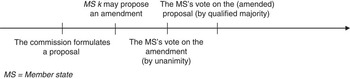
Under consultation, the Commission first proposes a policy. Next, the Commission proposal is sent to the Council. In the Council, member states can propose amendments. We assume for simplicity that only one member state k is selected to propose an amendment, and that it can decide whether or not to use that opportunity. Amendments need unanimity in the Council for approval. At the end of the procedure, the Council votes on the (amended) proposal. Approval by a qualified majority in the Council is required for adoption. If the proposal is adopted, it becomes EU law. Otherwise the status quo prevails. Figure 1 shows the sequence of events under consultation.
The sequence of events under the consultation procedure

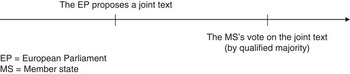
Under co-decision, the European Parliament proposes a joint text, as shown in the first step of Figure 2.Footnote 21 If it is approved by a qualified majority in the Council, it is adopted. Otherwise, the status quo prevails. The model incorporates complete and perfect information.Footnote 22 We use the sub-game perfect Nash equilibrium concept.
The sequence of events under the co-decision procedure

Legislative Activity and Gridlock
We next look at the conditions under which the EU manages to adopt legislation in period t under each of the two main legislative procedures: consultation and co-decision. Under consultation, the Commission needs the support of a qualified majority in the Council for the adoption of its proposal in the last step of the procedure. The Commission then focuses on the relevant pivotal member state, since any proposal that wins its support can be adopted in the Council. If the Commission wants to move to the right (left), the relevant pivotal member state is member state a (b). The Commission thus only considers the policies that this member state prefers to the status quo. Not all proposals that are preferred to the status quo by the relevant pivotal member state make it to the last step of the procedure, however, because they can be amended by unanimity in the second and third steps of the procedure. Such proposals that are to the left or right of the ideal policies of all member states are successfully amended, and the amended proposal will be between the ideal policies of the two extreme member states. When formulating its proposal in the first step of the procedure, the Commission thus considers the policies that are (1) preferred to the status quo by the relevant pivotal member state and (2) between the ideal policies of the two extreme member states. The Commission successfully proposes the policy it prefers most from this set of policies.
So under what circumstances does consultation lead to gridlock? To be adopted, proposals need to be preferred to the status quo by a qualified majority. If the status quo is to the right (left) of member state a (b), there is no qualified majority in favour of a move to the right (left). That is, if the status quo is in the set [pa,pb], gridlock results. The status quo may also prevail if there are policies that a qualified majority in the Council strictly prefers to the status quo, but the Commission prefers the status quo to such policies. This occurs if the status quo is between the ideal policies of the Commission, on the one hand, and the pivotal member states on the other hand: if pc ≤ SQ < pa or pb < SQ ≤ pc . The Commission and the pivotal member states then want to move the status quo in opposite directions. Hence, the status quo prevails in interval [min{pa,pc },max{pb,pc}] unless all member states want to move in the same direction away from the status quo.
If all member states do want to move in the same direction, that is, SQ < p1 or pm < SQ, they can successfully amend Commission proposals. The gridlock interval under consultation is then equal to the interval GICONS = [min{pa,pc},max{pb,pc}] ∩ [p1,pm] = [max{p1,min{pa,pc}}, min{pm,max{pb,pc}}]. The status quo prevails if it is in this interval. If the status quo is not in this interval, the EU is able to adopt legislation.
Turning to co-decision, in the last stage of the procedure a joint text requires approval by a qualified majority in the Council. At the first stage, the European Parliament thus considers the policies that the relevant pivotal member state prefers to the status quo, and successfully proposes, as a joint text, the policy it prefers most from among these policies.
Under what circumstances does co-decision lead to gridlock? Proposals need to be preferred to the status quo by the European Parliament and a qualified majority in the Council to be adopted. If no policy is preferred to the status quo by the European Parliament and a qualified majority – that is, if the status quo is between the ideal policies of the European Parliament and the two pivotal member states – gridlock results. The gridlock interval for an issue under co-decision is then equal to the interval GICOD = [min{pa,pp }, max{pb,pp}].
DETERMINANTS OF GRIDLOCK
As discussed, our theory suggests that equilibrium policies depend on two main factors: actors’ preferences and institutional rules. We now analyse how these factors affect gridlock.
Actors’ Preferences
In the previous section, we determined the gridlock intervals for an issue in period t under consultation and co-decision. Under consultation, the gridlock interval widens as the pivotal member states are farther apart, and as the extreme member states and the Commission are farther away from the midpoint between the two pivotal member states’ ideal policies. Under co-decision, meanwhile, the gridlock interval expands as the pivotal member states are farther apart, and as the European Parliament is farther away from the midpoint between the two pivotal member states’ ideal policies. More preference heterogeneity thus hinders legislative activity on an issue under both consultation and co-decision.
At the start of each period, the Commission considers on what issues legislative activity is possible. It then studies the equilibrium policies that will emerge on these issues, and the utility it will derive from those policies. It chooses the issue that yields the largest utility increase, or smallest utility decrease, for itself.Footnote 23 If the status quo is in the gridlock interval on each issue, no legislative activity occurs during the period. Thus there is less legislative activity and more gridlock if preferences are more heterogeneous. This leads to the following testable hypothesis:
Hypothesis 1: Legislative activity increases as the gridlock interval contracts. The gridlock interval on dimension i contracts as (1) the ideal policies of the pivotal member states on that dimension are closer together, (2) the ideal policies of the Commission and the extreme member states are closer to the midpoint between the pivotal member states’ ideal policies (under consultation) and (3) the European Parliament's ideal policy is closer to the midpoint between the pivotal member states’ ideal policies (under co-decision).
We now examine more closely how the preferences of the Commission, the European Parliament and the member states affect gridlock. The Commission is appointed by the member state governments and the MEPs for a five-year term after each European Parliament election. As new commissioners take office, their preferences are likely to be different from those of their predecessors. Occasionally, individual commissioners are replaced during a Commission term. Commissioners may also change their preferences during their terms.
Since the Commission does not propose the joint text or vote on it under co-decision, legislative activity does not depend on its preferences under this procedure. However, under consultation it does. Under consultation, if the old and new Commission are both located between the two pivotal member states, the gridlock interval is not affected by the investiture of a new Commission. But if the old (new) Commission is located between the two pivotal member states, but the new (old) Commission is not, the gridlock interval expands (contracts). And if neither the old nor the new Commission is located between the two pivotal member states, gridlock increases (reduces) if the new Commission is farther away from (closer to) the midpoint between the two pivotal member states.
The European Parliament is directly elected for a five-year term. A newly elected Parliament is likely to have different preferences from its predecessor. As was the case for commissioners, occasionally individual MEPs are replaced during their terms, and sitting MEPs may change their preferences after their election. In our model, the preferences of the European Parliament do not affect legislative activity under consultation. Under co-decision, by contrast, the effect of changing European Parliament preferences is the same as the effect of changes in Commission preferences under consultation.
Finally, member states are represented in the Council by national government ministers. In contrast to the European Parliament and the Commission, Council members are not all re-elected or reappointed at the same time. Member state representatives change at various moments during a Commission's term, whenever there is a change of government in a member state, as a result of national elections or the formation of a new government, or if there is a reshuffle of cabinet seats.
A change in a member state's preferences affects legislative activity only if it leads to a different preference configuration of the pivotal and extreme member states. Such a different configuration emerges when one of the pivotal or extreme member states changes its preferences (while remaining pivotal or extreme) or when another member state becomes pivotal or extreme as a result of a preference change. In either case, the result of a change that affects the preferences of a pivotal member state is similar to the result of the changes in Commission or European Parliament preferences discussed above.Footnote 24 The result of a change that affects the preferences of an extreme member state is straightforward: if the (possibly) new extreme member state is farther from the closer pivotal member state, gridlock increases. Otherwise it reduces.
Changes to Institutional Rules
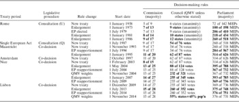
Table 1 shows the evolution of the EU's legislative rules between the entry into force of the Treaty of Rome and the end of the 2009–14 European Parliament. So, for example, between 1958 and 1986 the EU adopted legislation using the consultation procedure and unanimous agreement amongst the then nine member states in the Council. The majorities in the Commission and the European Parliament were not relevant for determining the gridlock interval at that time. Then, between July 1987 and October 1993, the Single European Act (SEA) era, the EU adopted most legislation using the consultation procedure and QMV in the Council (which at that time was fifty-four out of seventy-six votes). After the entry into force of the Maastricht Treaty in November 1993, the co-decision procedure became the most important legislative procedure, which requires a qualified majority in the Council and a simple majority in the European Parliament.
Evolution of the EU's Legislative Decision-Making Rules

Note: changes to the decision-making rules in the Commission, the Council or the EP are indicated in bold. Consultation (U) is the consultation procedure with unanimity in the Council. Consultation (Q) is the consultation procedure with QMV in the Council.
Whether there is more gridlock under the consultation or co-decision procedures depends on the relative locations of the ideal policies of the European Parliament, the Commission, and the pivotal and extreme member states. If the European Parliament and the Commission are both located between the two pivotal member states, the extent of gridlock is the same under both procedures. If the Commission is between the pivotal member states, but the European Parliament is not, the gridlock interval is wider under co-decision than under consultation. But if the European Parliament is between the pivotal member states and the Commission is not, then the gridlock interval is smaller under co-decision than under consultation. If neither the Commission nor the European Parliament is located between the pivotal member states, and the Commission (or the extreme member state that is on the same side of the pivotal member states as the Commission) is closer to (farther from) the midpoint of the ideal policies of the pivotal member states than the European Parliament is, the gridlock interval is wider (smaller) under co-decision. Hence, our theory predicts that the introduction of co-decision has an impact on legislative activity insofar as the introduction of the new procedure affects the size of the gridlock interval. It does not predict any impact beyond that.
Even though the Treaty of Rome provided for QMV, in practice it was not used until the SEA. Then, each subsequent treaty extended its use. There is more gridlock when unanimity is used than when QMV is used, both under consultation and co-decision. Under consultation, there is gridlock under unanimity if the status quo is between the ideal policies of the two extreme member states on that issue; that is, if it is in the set [p1,pn]. This is a superset of the gridlock set GICONS under QMV. Under co-decision, there is additional gridlock under unanimity if the European Parliament is not between the ideal policies of the two extreme member states and the status quo is between the European Parliament and the extreme member states. The gridlock set is then [min{p1,pp }, max{pn,pp }], which is a superset of the gridlock set GICOD under QMV. Thus our theory predicts that the move from unanimity to QMV has a positive impact on legislative activity only insofar as it affects the gridlock interval.
Finally, it is often claimed that EU enlargement has made decision making more cumbersome and led to a decrease in legislative activity. Our theory predicts that the impact of adding more member states depends on the location of the ideal policies of these new member states. If the gridlock interval expands as a result of their entry into the EU, legislative activity can be expected to decrease. Otherwise it will increase. For example, the gridlock interval expands in a policy area if unanimity is used and the new member states all have ideal policies that are to the left of the old member states. An increase in preference heterogeneity thus leads to an expansion of the gridlock interval. If, by contrast, QMV is used and all new member states have ideal policies between the pivotal member states, the gridlock interval decreases and legislative activity increases. Our theory therefore predicts that EU enlargement has an impact on legislative activity only insofar as it affects the gridlock interval.
EMPIRICAL ANALYSIS
To test these ideas, we developed a method for calculating the size of the gridlock interval in EU legislative institutions during a particular period, and then analysed the relationship between the size of this interval and the number of EU laws adopted. According to our theory, the location of the status quo on a particular policy issue, and whether this point is inside or outside the gridlock interval, should predict whether the policy can be changed in a particular period. One possible empirical operationalization of this would be to look at the location of policy status quos in a particular period, to see whether these policies are moved into the gridlock interval. Yet such an operationalization is very difficult in any context.Footnote 25 Furthermore, there are several good reasons why the volume of legislation in a particular period is a reasonable way of testing our theory in the EU context.
First, because much of the data we are looking at relates to new EU policies and the building of the single market, policy status quos are not likely to be limited to particular parts of the policy space, which are then freed up when the gridlock interval changes. Existing policy status quos are likely to be reasonably evenly distributed on a left-right dimension, because some EU policies lead to the de-regulation of existing standards, whereas other policies lead to the adoption of new regulatory standards.
Secondly, because of the way EU decision making works and because of the different electoral timetables of the member states and institutions, it is impossible to identify a period in EU politics in which the gridlock interval is fixed for a long enough period of time for all existing policies outside this interval to be moved into the interval. Specifically, it would not be reasonable to treat each six-month period, year, or European Parliament or Commission term as a clear ‘period’ during which all status quos from outside the gridlock interval are likely to be brought into the interval.
Instead, we can assume that the size of the gridlock interval in a particular period influences EU institutions’ ability to adopt a given policy at that time, all other things being equal. So, for simplicity, our dependent variable is the number of legislative acts adopted by the EU in any six-month period between July 1979 and June 2009.Footnote 26 A six-month period is a more appropriate unit of analysis than a calendar year due to the six-monthly rotating presidency of the Council and because the European Parliament is elected in June every five years. We calculated the number of legislative acts adopted in each period from Frank Häge's EUPOL dataset.Footnote 27 As a robustness check, we use König, Luetgert and Dannwolf's alternative measure of EU legislative activity, which covers the 1984–2002 period.Footnote 28
To calculate the size of the gridlock interval in a six-month period we proceeded as follows. First, we identified the main decision-making rules that apply in each six-month period, as described above and in Table 1. In most of these periods, several different rules are used at the same time. For example, during the period of the SEA, the co-operation and consultation procedures were used for different policy issues, and under the period of the Maastricht Treaty, the co-decision and consultation procedures were used for different policy issues. Also, in most periods, some legislation was adopted by unanimity in the Council while other legislation was adopted by QMV, depending on the legislative procedure.
To test our model, though, we needed to make an assumption about the main procedural rules used in each period; we used the procedures as shown in Table 1. Nevertheless, by making this assumption, we introduced a certain measurement error, which reduced the likelihood that we will find significant results. As a robustness check, we also tested whether the results hold if we assume that co-operation rather than consultation was the main procedure used during the SEA period.
Secondly, having identified the procedures used in each six-month period, which in turn determined the pivotal actors under each procedure, we then calculated the location of each of the actors. Here, again, we made a simplifying assumption: that these actors are located on a left-right policy dimension. This is not an unreasonable simplification. There is some evidence that the left-right dimension is present in roll-call voting in the Council,Footnote 29 and considerable evidence exists that the left-right is the dominant dimension of roll-call voting in the European Parliament.Footnote 30 Nevertheless, most scholars of EU politics assume that the EU policy space is multidimensional, and there is considerable evidence of this.Footnote 31 For example, expert interviews on the locations of actors in EU decision making have found that actors’ positions in the Council correlate with underlying pro/anti-integration preferences or EU budget contributions.Footnote 32
However, we estimate actors’ positions on a single left-right dimension for several reasons. Measuring the gridlock interval in more than one dimension is a non-trivial exercise, and would introduce a further level of complexity when interpreting the empirical results. Also, estimates of EU actors’ positions on a pro-/anti-Europe dimension cover a shorter time period and are less reliable than estimates of actors’ positions on a left-right dimension. And since most EU legislation since 1979 has related to the creation and regulation of the single market, it is reasonable to assume that politicians’ preferences on many EU policies (such as environmental or social standards) are influenced by their underlying left-right policy preferences. Yet if EU policy making is in fact multidimensional, then assuming that it is one-dimensional introduces measurement error, which in turn reduces the likelihood that we will find significant results by making this simplifying assumption.
To calculate the positions of actors on the left-right dimension, we start with the information on party and government positions in Döring and Manow's ParlGov dataset.Footnote 33 Döring and Manow use ‘expert judgment’ data from a range of sources to estimate the left-right position of each political party in the EU over time on a 0 to 10 left-right scale.Footnote 34 Using these data, the position of each government in the Council was calculated as the average position of the parties in a government, weighted by the share of the parliamentary seats of the parties in government. From these data we then calculated the location of the pivotal and extreme governments in the Council on the left-right dimension in each six-month period.
For the Commission, we assumed that each commissioner was located at the same position on the left-right dimension as the national party to which he or she belonged. We do not believe that each commissioner has exactly the same positions as his or her party. Nevertheless, because almost all commissioners are career party politicians, it is not unreasonable to assume that the left-right location of a commissioner's national party is correlated with his or her position on this dimension. From these data we then worked out the location of the median commissioner on the left-right dimension in each six-month period.
For the European Parliament, we assumed that each MEP has the same left-right position as his or her national party. We then calculated the median member of each political group in the European Parliament and identified the median political group on the left-right dimension in each six-month period; we used this as the left-right location of a majority in the European Parliament in a particular period.
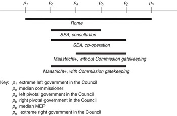
From the left-right positions of the key member states and the median members of the European Parliament and the Commission, we then calculated the size of the gridlock interval in each six-month period between July 1979 and June 2009. For this we followed the inferences of the theoretical model. This is illustrated in Figure 3. So for the period of the Rome Treaty, when legislation was adopted by consultation and unanimity, the gridlock interval was the set [p1,pn] of policies between the extreme left and right governments.
Illustration of the gridlock intervals

For the period of the SEA, when we assume that most legislation was passed under the consultation and QMV, the gridlock interval was the set [min{pa,pc},max{pb,pc}] between the position of the left pivotal government in the Council or the Commission and the position of the right pivotal government in the Council or the Commission.Footnote 35 As a robustness check, we also calculate gridlock intervals for the period of the SEA, assuming that co-operation was the main decision-making procedure. Under this procedure, the European Parliament had a veto right, and the gridlock interval was thus the set [min{pa,pp,pc},max{pb,pp,pc}] of policies between the furthest left of three actors (the Commission, the European Parliament and the left pivotal government in the Council) and the furthest right of three actors (the Commission, the European Parliament and the right pivotal government). So in the hypothetical example in Figure 3, the gridlock interval under the consultation procedure is the distance between pc and pb , and under the co-operation procedure it is the distance between pc and pp .
For the period following the Maastricht Treaty, when we assume that most legislation was adopted using the co-decision procedure, the gridlock interval was the set [min{pa,pp}, max{pb,pp}] of policies between the left pivotal government in the Council or the European Parliament and the right pivotal government in the Council or the European Parliament. As a robustness check, we also calculate gridlock intervals for the period after the Maastricht Treaty, assuming that the Commission had gatekeeping power. In this case, the gridlock interval in this period was the same as under the co-operation procedure. So in the hypothetical example in Figure 3, the gridlock interval under the co-decision procedure without Commission gatekeeping is the distance between pa and pp , and under the co-decision procedure with Commission gatekeeping it is the distance between pc and pp . Finally, in the statistical analysis we include a number of control variables that are often broached to influence the volume of legislation adopted by the EU in a given period.
As discussed, we predict that these variables should not have an impact on legislative activity independently of their effects on the size of the gridlock interval. First, the No. of Member States is simply a count of the number of EU members in a six-month period, which ranges from nine in July 1979 to twenty-seven in June 2009.
Secondly, the variable EP Cycle captures the point in the term of a European Parliament: the first six-month period in a parliamentary term takes the value 1, the second six-month period takes the value 2, and so on until the final six-month period before a European Parliament election takes the value 10. This variable captures an effect identified by the European Parliament's research division, in which there is an increase in legislative activity during a parliamentary term.Footnote 36 Fewer laws tend to be passed at the beginning of a parliamentary term, because the process of forming political groups and committees delays the passage of legislation. Then, toward the end of a parliamentary term, the Commission and Council try to get as many laws passed as possible before the European Parliament breaks for the election period and the formation of the new Parliament.
Thirdly, the variable Part Year captures whether a six-month period is the first half of a year (coded 0) or the second half (coded 1). This variable accounts for the EU agenda, in which annual budgetary issues, for example, are usually resolved in the second half of the year.
Fourthly, the variable Big State Presidency equals 1 if one of the larger member states (Germany, France, United Kingdom, Italy or Spain) held the six-monthly rotating presidency of the Council, and 0 otherwise. This variable controls for the possibility that the larger EU states are able to push through more legislation during their period at the helm of the Council than smaller states are.
Fifthly, the variable EU Public Support captures the changing level of support for the EU over time. If the EU institutions respond to the ‘policy mood’ of the public, one might expect the EU to adopt more legislation when public support for the EU is higher, and less legislation when public support is lower. Indeed, Franklin and Wlezien and Toshkov find a relationship between more public support for the EU and more legislative action by the EU, at least until the 1990s.Footnote 37 This is similar to Eriksson et al.'s claim about the effect of the policy mood of the US public on the activities of the US Congress.Footnote 38 For this variable we use the ‘membership’ question in the Eurobarometer (EB) survey from a particular period (Spring EBs for January–June and Autumn EBs for July–December), and identify the (weighted) percentage of people in the EU that regards their country's membership of the EU as a ‘good thing’ in the six-month period before the six-month period of observation – to take into account a likely ‘lag’ effect of public opinion on the EU institutions. We use the Mannheimer EB Trend File for all periods up to Spring 2002, and each separate EB data file for all periods since August 2002.
Sixthly, the variable Before Enlargement captures the likely effect of the final six-month period before a new member state or group of member states joined the EU. This measure takes into account the oft-observed fact that the EU tried to pass a lot of legislation before the two enlargements to the Central and Eastern European states in the 2000s, perhaps with the expectation from the Commission (and some existing member states) that some legislative acts might be more difficult to pass in an enlarged Council.
Finally, in some models we include dummy variables for each separate institutional period. The variable Rome captures the period of the Treaty of Rome, and is coded 1 from the start of the dataset until January–June 1987, and 0 thereafter. The variable SEA captures the period of the SEA, and is coded 1 from July–December 1987 until July–December 1993, and 0 otherwise. The variable Maastricht+ captures the effect of the entry into force of the Maastricht Treaty, and is coded 1 from January–June 1994 until the end of the data, and 0 otherwise. These dummy variables account for the increasing policy competences of the EU as a result of each of these treaty reforms. Related to this, our theory predicts that legislative activity decreases over time, but that the deepening of the EU that resulted from the SEA and the Maastricht Treaty led to an increase in EU legislation. Descriptive statistics for all the variables are shown in Table A1 in the Appendix.
RESULTS
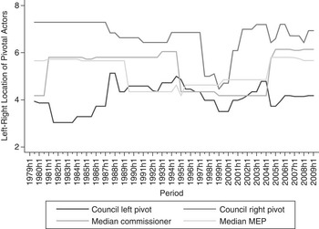
To get a sense of some of the patterns in the data, Figure 4 shows the locations of the pivotal actors in the EU during our thirty-year period. The gap between the extreme left and right governments in the 1980s was considerable. After the entry into force of the SEA in 1987, the two relevant actors in the Council shifted closer together, because the identity of these actors changed from the two extreme governments to the two pivotal governments as a result of the change form unanimity to QMV. The pivotal governments in the Council then became very close together in the late 1990s, as a result of a shift to the left in a large number of member states. The gap between the two pivotal governments grew again in the early 2000s. The European Parliament and the Commission, meanwhile, were between the two pivotal governments in the Council in most periods, except between 1989 and 1996, when the European Parliament shifted considerably to the left, for short periods in 1995–96 and 2002–04, when the median commissioner was further to the left than both pivotal governments, and between 1999 and 2000, with the European Parliament was briefly to the right of the pivotal governments in the Council.
Locations of the pivotal actors in EU decision making

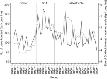
The light grey line (on the inverted right-hand scale) in Figure 5 illustrates how these shifting positions affected the size of the gridlock interval. In general, the gridlock interval was larger under the Rome Treaty, much smaller under the SEA, and then shifted considerably during the period following the Maastricht Treaty, and was at its smallest between 1997 and 2000. As Figure 5 also shows, the volume of legislation adopted by the EU appears to broadly follow the changes in the gridlock interval sizes, as shown by the dark grey line (on the left-hand scale), although with much higher variation.
Gridlock interval size and legislative activity

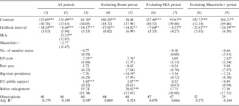
Table 2 presents the main results.Footnote 39 The size of the gridlock interval is statistically significant in all model specifications. Specifically, the bigger the gridlock interval, the less legislation the EU passed. In Model 1 for example, the size of the gridlock interval alone explains about 18 per cent of the variance in the volume of legislation adopted by the EU. In addition, a one-unit increase in the size of the gridlock interval (measured on a ten-point scale) corresponds to fourteen fewer pieces of legislation passed by the EU in a six-month period.
Gridlock Interval and Number of Laws Adopted

Note: the dependent variable is the number of laws adopted by the EU in a six-month period, between 1979 and 2009. OLS regression. Standard errors in parentheses. In Model 2, the Rome period is the baseline. In Model 5, the No. of member states variable is excluded because it is correlated with the size of the gridlock interval from the SEA onwards. *p ≤ 0.10, **p ≤ 0.05, ***p ≤ 0.01.
As Model 2 shows, moreover, the size of the gridlock interval remains significant even when controlling for changes to the decision-making rules, as represented by the SEA and Maastricht+ variables. Adding these two dummy variables controls for all periods after the extension of QMV in the SEA. Even with these variables included, a larger gridlock interval leads to fewer legislative acts adopted. Also, as the other models show, dropping one or other of the three institutional periods does not affect the general result. In other words, changes in the size of the gridlock interval within in each institutional period influence, as a result of the changing policy positions of the pivotal actors in the EU institutions, the volume of legislation adopted by the EU. Excluding the Rome period reduces the model's explanatory power because a large proportion of the variance in the dependent variable is explained by the shift from unanimity to QMV, as Figure 5 illustrates.
Regarding the other variables, the difference between the first and second halves of a year is not significant. In addition, less legislation tended to be adopted when one of the big member states held the Council presidency, although this is not significant in all models. In contrast, more laws have been adopted toward the end of European Parliament terms, at least since the SEA. Furthermore, since the SEA, higher public support for the EU has correlated with more legislative action, as others have found.
We also undertook a series of robustness checks (see Table A2 in the Appendix). We use an alternative measure of the dependent variable: König et al.'s measure of the number of laws adopted by the EU between 1984 and 2002. We use an alternative measure for the key independent variable: using left-right party positions from coding party manifestos.Footnote 40 And we looked at three alternative assumptions about the operation of the legislative rules: (1) that most legislation in the SEA period was adopted by the co-operation procedure, (2) that the Commission has gatekeeping power under the co-decision procedure and (3) that the Council is dominant and the Commission and Parliament can be ignored.Footnote 41 Our key results in Table 2 are robust to these alternative measures and assumptions: a larger gridlock interval corresponds with fewer legislative acts.
Of particular note is the fact that the magnitude of the effect of the gridlock interval is smaller if the interval is measured only in the Council, as opposed to including the Parliament and the Commission as pivotal actors. This finding suggests that the preferences of the EU's supranational institutions influence EU legislative outcomes over and above the preferences of the pivotal member states in the Council. This is an interesting result, given the fact that the European Parliament and/or the Commission were located outside the interval between the two pivotal member states in the Council in only nineteen of the sixty periods we analysed, as Figure 1 shows. The results suggest, though, that this was enough to make a difference. Put another way, less legislation was adopted in the early 1990s because the median MEP was to the left of the pivotal governments in the Council (under QMV) than would have been the case had the European Parliament not had power under the co-decision procedure.
Finally, we also looked at the effect of the gridlock interval on the volume of legislation proposed by the Commission (Table A2). The results suggest that the Commission is strategic when considering legislative proposals, in that it proposed less (more) legislation when the gridlock interval was larger (smaller). However, the magnitude of the relationship between the size of the gridlock interval and the volume of legislation proposed is smaller than the magnitude of the relationship between the size of the gridlock interval and the volume of legislation adopted. Interestingly, though, the results on some of the control variables are different in this model than in the other models. In particular, whereas the effect of the European Parliament election cycle influences the volume of legislation adopted, it has no effect on the volume of legislation proposed. Also, whereas a big member state holding the Council presidency has a negative effect on the volume of legislation adopted, a big member state holding the Council presidency has a positive effect on the volume of legislation proposed, although these results are not statistically significant.
CONCLUSION
Intuitively, one might think that enlargement of the EU from six to twenty-eight member states and changes to the procedural rules that have added the European Parliament as a veto player have made it more difficult for the EU to adopt policy. Our theory challenges these intuitions. As in other multi-actor legislative environments, such as the US presidential system or coalition governments in parliamentary systems, the ability to adopt legislation depends on the preferences of the key actors, the rules governing the relative powers of these actors and the location of existing polices. These factors together determine the size of the set of policies that can be moved, and conversely the size of the set of policies that cannot be moved: the gridlock interval. In our approach, the number of actors or the decision-making rules only affect policy outcomes insofar as they influence the relative size of the gridlock interval.
In the EU context, our approach is consistent with the view of Tsebelis and Garrett, amongst others, that there have been three main periods in the development of the EU's decision-making rules: unanimity in the Council in the Rome Treaty period, QMV in the Council plus a new role for the Commission during the SEA period, and a new role for the Parliament in the post-Maastricht period.Footnote 42 So, for example, consistent with the conventional wisdom about the SEA, our approach explains how the shift to QMV reduced the size of the gridlock interval, and therefore led to the adoption of more legislation.
In contrast to existing research, though, our approach also suggests that within each of these periods, the size of the gridlock interval should change significantly as the relative preferences of the Commission, the European Parliament and the pivotal member states change. So, for example, we argue that the large volume of legislation adopted by the EU in the late 1980s was a result of the combined effects of the new institutional rules introduced by the SEA (such as QMV in the Council) and the relatively close positions of the pivotal actors in the institutions at that time. Put another way, the effect of Jacques Delors was at least in part due to the fortuitous institutional and political context during his presidency of the Commission.
Our empirical analysis of EU legislative activity in every six-month period between 1979 and 2009 supports this perspective. We find compelling evidence that as the gridlock interval in the EU increased (decreased) from one six-month period to the next, the legislative activity of the EU decreased (increased), both between the institutional periods and within each of the institutional periods. For example, a decline in the size of the gridlock interval in the late 1990s, as a result of a shift to the centre-left across the EU at that time, corresponded to an increase in EU legislative activity. Then, in the early 2000s, as the EU Council became more heterogeneous as more centre-right governments were elected, and following the election of a centre-right majority in the European Parliament, the gridlock interval increased and EU legislative activity declined.
Moreover, these results are perhaps surprising, given the simplifying assumptions we had to make in the empirical estimation about the uni-dimensionality of EU politics and the use of a single main legislative procedure in each period. Given the inevitable errors in the measurement of our key independent variable that result from these simplifications, the magnitude of our key results is probably at the lower bound of the true relationship between gridlock size and EU legislative outputs.
Finally, our theory also suggests that the EU should adopt particular types of policies in particular periods. So if the pivotal actors are close together on the centre-left, as they were in the late 1990s, the EU should not only adopt more policy, but should also move existing policy status quos in a leftward direction. Conversely, if the pivotal actors are close together on the centre-right, as they were in the late 2000s, the EU should once again adopt more policy than in the early 2000s (when the gridlock interval was larger), but should also move existing policy status quos in a rightward direction. Hence, building on our theory and evidence, future research could look at how the substantive content of EU policy has changed over time in response to the size of the gridlock interval and the preferences of the key actors.