1. Introduction
Many planets and stars are surrounded by magnetic fields, which we believe are created by flows in their electrically conducting fluid interiors. This process is studied in dynamo theory, and ever since its advent, a central question has been to identify what makes a flow an efficient dynamo. Some will say it has to be helical, others will demand shear and again others will say it is chaotic stretching of fluid parcels that we need. Different dynamo mechanisms may be important in different physical situations, but as a prelude to more elaborate calculations we can try to ask a very simple question: can we identify the flows that act as the best (optimal) dynamos for a given geometry? What are their characteristics and is there something that we can learn from them?
The search for optimized dynamos is not new and has been adopted in particular in preparation for experimental dynamo campaigns (Riga, Karlsruhe, Madison, VKS). Most of these studies, however, consider flows that vary in small- to mid-scale
 $O(10{-}100)$
parameter spaces and/or use symmetrical flows to reduce the numerical cost. Several works have optimized radial structures of axisymmetric flows: Love & Gubbins (Reference Love and Gubbins1996) for Kumar–Roberts flows in 3D parameter space, Holme (Reference Holme2003) for Dudley–James flows in a 26D phase space, Stefani, Gerbeth & Gailitis (Reference Stefani, Gerbeth and Gailitis1999) for the Riga dynamo. In a more advanced study by Khalzov et al. (Reference Khalzov, Brown, Cooper, Weisberg and Forest2012) dedicated to the Madison Plasma Device Experiment, it is not the axisymmetric flow that is optimized, but an axisymmetric boundary forcing in a 10-parameter phase space. Non-axisymmetric flow optimizations are quite rare; however, Alexakis (Reference Alexakis2011) optimized ABC flows in a 2D phase space.
What should one do if one wished to optimize the full spatial structure of a flow? Clearly it is necessary to find an efficient way to walk through a potentially extremely high-dimensional parameter space. Such a path can be provided by variational optimization methods (Lions Reference Lions1970). These methods have been frequently used in the inverse problems that are solved by seismologists (Tarantola Reference Tarantola1984; Tromp, Komattisch & Liu Reference Tromp, Komattisch and Liu2008), but also in the geodynamo context, variational data assimilation techniques (Li, Jackson & Livermore Reference Li, Jackson and Livermore2011, Reference Li, Jackson and Livermore2014) have been proposed to infer dynamical information concerning the Earth’s interior. In the hydrodynamical context, the variational optimization method has recently provided new insights into the problem of subcritical transition (Pringle & Kerswell Reference Pringle and Kerswell2010; Pringle, Willis & Kerswell Reference Pringle, Willis and Kerswell2012; Duguet et al. Reference Duguet, Monokrousos, Brandt and Henningson2013; Kerswell, Pringle & Willis Reference Kerswell, Pringle and Willis2014).
In the present context of optimized dynamo action, it is precisely this type of variational method that allowed Willis (Reference Willis2012) to solve the optimized dynamo problem. Within a huge class (
 ${\sim}10^{5}$
-dimensional parameter space) of stationary incompressible flows that fitted in a periodic cubic box, minimal dynamo thresholds and accompanying flows and fields were identified. The minimal dynamo thresholds for the optimized dynamos as reported by Willis are among the lowest ones ever observed and can be compared with existing lower bounds for dynamo action (Backus Reference Backus1958). This possibility to numerically quantify the precise lower bound for dynamo action is indeed quite exceptional and certainly very new in dynamo theory.
In this article, we extend the work initiated by Willis (Reference Willis2012). The search for optimal dynamos in periodic fluid domains was a critical first step, but if we want to reach towards geophysically or experimentally realizable flows, it is necessary to bound the flows within finite fluid domains and to impose boundary conditions on the magnetic field. This presents a serious challenge since boundary conditions are not often trivially implemented in these optimization methods. For the moment, we still consider cubic domains instead of more planetary-like settings, but we find a first way to build the most efficient dynamos in domains with boundaries. Our flows will remain inside the box and magnetic fields will satisfy either perfectly conducting or pseudovacuum conditions on the sidewalls. The same types of conditions were studied by Krstulovic et al. (Reference Krstulovic, Thorner, Vest, Fauve and Brachet2011), and the advantage is that one can still use periodic box codes to perform the calculations. We will explain the method in detail, in particular the parts related to the boundary conditions. We aim to find optimal dynamos, and as a by-product the minimal critical magnetic Reynolds numbers for dynamo action. An unexpected outcome of this study is the fact that when a flow
 $\boldsymbol{U}$
is an optimal dynamo with a given set of boundary conditions, the inverted flow
 $-\boldsymbol{U}$
is also an optimal dynamo for a complementary but different set of boundary conditions. We can explain this using an argument close to recent work by Favier & Proctor (Reference Favier and Proctor2013).
2. Problem and method
2.1. Objective function
The variational optimization method (Lions Reference Lions1970; Talagrand & Courtier Reference Talagrand and Courtier1987) is strongly inspired by Willis (Reference Willis2012). We choose to optimize the asymptotic growth of the magnetic energy in the cube directly to select the most efficient dynamo. More precisely, inside the fluid domain
 $\mathscr{V}$
, which is a cubic box of unit size, we search for the best stationary flows
 $\boldsymbol{U}(\boldsymbol{x})$
and initial magnetic fields
 $\boldsymbol{B}_{0}=\boldsymbol{B}(\boldsymbol{x},0)$
that give the maximal magnetic energy growth at a large but finite time
 $T$
. This results in the following objective functional with various constraints:
 $$\begin{eqnarray}\displaystyle \mathscr{L} & = & \displaystyle \ln \langle \boldsymbol{B}_{T}^{2}\rangle -{\it\lambda}_{1}(\langle (\boldsymbol{{\rm\nabla}}\times \boldsymbol{U})^{2}\rangle -1)-{\it\lambda}_{2}(\langle \boldsymbol{B}_{0}^{2}\rangle -1)\nonumber\\ \displaystyle & & \displaystyle -\,\langle {\it\Pi}_{1}\,\boldsymbol{{\rm\nabla}}\boldsymbol{\cdot }\boldsymbol{U}\rangle -\langle {\it\Pi}_{2}\boldsymbol{{\rm\nabla}}\boldsymbol{\cdot }\boldsymbol{B}_{0}\rangle \nonumber\\ \displaystyle & & \displaystyle -\,\int _{0}^{T}\langle \boldsymbol{B}^{\dagger }\boldsymbol{\cdot }[\partial _{t}\boldsymbol{B}-\boldsymbol{{\rm\nabla}}\times (\boldsymbol{U}\times \boldsymbol{B})+Rm^{-1}\boldsymbol{{\rm\nabla}}\times \boldsymbol{{\rm\nabla}}\times \boldsymbol{B}]\rangle \,\text{d}t.\end{eqnarray}$$
We denote here
 $\langle \cdots \rangle =(1/\mathscr{V})\int _{\mathscr{V}}\cdots \text{d}\mathscr{V}$
as the integral over the box. The first term expresses that we maximize the logarithm of magnetic energy at time
 $T$
, since at large
 $T$
the magnetic energy can be described by an exponential function. We write as shorthand
 $\boldsymbol{B}_{T}=\boldsymbol{B}(\boldsymbol{x},T)$
for the final magnetic field. In the non-dimensional setting, the fluid flow has to be normalized (constrained by
 ${\it\lambda}_{1}$
), here by an enstrophy or dissipation norm. As noted by Willis, the alternative normalization that fixes the kinetic energy
 $-{\it\lambda}_{1}(\langle \boldsymbol{U}^{2}\rangle -1)$
is problematic as discontinuous flows with unlimited shear may then be picked up by the optimizer. This problem is avoided by using the dissipation norm. The flow also has to be a solenoidal (constrained by
 ${\it\Pi}_{1}$
) field. The magnetic field satisfies the induction equation at all times (constrained by
 $\boldsymbol{B}^{\dagger }$
). It is sufficient to impose that the initial magnetic field
 $\boldsymbol{B}_{0}$
is solenoidal (constrained by
 ${\it\Pi}_{2}$
), since solenoidality is preserved by the induction equation, and therefore
 $\boldsymbol{{\rm\nabla}}\boldsymbol{\cdot }\boldsymbol{B}=0$
is guaranteed at all times. The maximization is not well defined unless the initial magnetic field amplitude is fixed (normalized) (constrained by
 ${\it\lambda}_{2}$
).
The functional was written immediately in non-dimensional form and depends on two non-dimensional numbers:
 $T$
, the time horizon, and
 $Rm$
, the magnetic Reynolds number, defined as
 $$\begin{eqnarray}\displaystyle Rm=SL^{2}/{\it\eta}. & & \displaystyle\end{eqnarray}$$
Here,
 $S$
is a measure for the dimensional enstrophy or typical shear magnitude,
 $L$
is the dimensional box size and
 ${\it\eta}$
is the magnetic diffusivity. Time is measured in units of
 $S^{-1}$
, space in units of
 $L$
, velocity in units of
 $SL$
and magnetic field units are arbitrary.
2.2. Boundary conditions
The crucial difference from Willis’ work is that we demand that
 $\boldsymbol{U}$
and
 $\boldsymbol{B}$
satisfy boundary conditions on the walls
 ${\it\Sigma}$
of the cubic box. We can impose these boundary conditions by adding supplementary constraints to
 $\mathscr{L}$
or we can limit the variations to classes of functions that meet a fixed set of boundary conditions. We choose the second approach.
Flows
 $\boldsymbol{U}$
are allowed to slip on the boundary but cannot penetrate it:
 $$\begin{eqnarray}\displaystyle \boldsymbol{n}\boldsymbol{\cdot }\boldsymbol{U}|_{{\it\Sigma}}=0, & & \displaystyle\end{eqnarray}$$
where
 $\boldsymbol{n}$
is the external unit normal everywhere on
 ${\it\Sigma}$
.
Magnetic fields
 $\boldsymbol{B}$
will satisfy either a perfectly conducting (T, tangential) or a pseudovacuum (N, normal) boundary condition, on each of the three pairs of parallel end plates. Out of eight possible configurations, we consider only four physically independent combinations:
 $$\begin{eqnarray}\displaystyle \underbrace{\begin{array}{@{}r@{}}\hat{\boldsymbol{x}}\times \boldsymbol{B}|_{x=0,1}=0,\\ \hat{\boldsymbol{x}}\boldsymbol{\cdot }\boldsymbol{J}|_{x=0,1}=0,\\ \hat{\boldsymbol{y}}\times \boldsymbol{B}|_{y=0,1}=0,\\ \hat{\boldsymbol{y}}\boldsymbol{\cdot }\boldsymbol{J}|_{y=0,1}=0,\\ \hat{\boldsymbol{z}}\times \boldsymbol{B}|_{z=0,1}=0,\\ \hat{\boldsymbol{z}}\boldsymbol{\cdot }\boldsymbol{J}|_{z=0,1}=0,\end{array}}_{\text{NNN}}\quad \underbrace{\begin{array}{@{}r@{}}\hat{\boldsymbol{x}}\times \boldsymbol{B}|_{x=0,1}=0,\\ \hat{\boldsymbol{x}}\boldsymbol{\cdot }\boldsymbol{J}|_{x=0,1}=0,\\ \hat{\boldsymbol{y}}\times \boldsymbol{B}|_{y=0,1}=0,\\ \hat{\boldsymbol{y}}\boldsymbol{\cdot }\boldsymbol{J}|_{y=0,1}=0,\\ \hat{\boldsymbol{z}}\boldsymbol{\cdot }\boldsymbol{B}|_{z=0,1}=0,\\ \hat{\boldsymbol{z}}\times \boldsymbol{J}|_{z=0,1}=0,\end{array}}_{\text{NNT}}\quad \underbrace{\begin{array}{@{}r@{}}\hat{\boldsymbol{x}}\times \boldsymbol{B}|_{x=0,1}=0,\\ \hat{\boldsymbol{x}}\boldsymbol{\cdot }\boldsymbol{J}|_{x=0,1}=0,\\ \hat{\boldsymbol{y}}\boldsymbol{\cdot }\boldsymbol{B}|_{y=0,1}=0,\\ \hat{\boldsymbol{y}}\times \boldsymbol{J}|_{y=0,1}=0,\\ \hat{\boldsymbol{z}}\boldsymbol{\cdot }\boldsymbol{B}|_{z=0,1}=0,\\ \hat{\boldsymbol{z}}\times \boldsymbol{J}|_{z=0,1}=0,\end{array}}_{\text{NTT}}\quad \underbrace{\begin{array}{@{}r@{}}\hat{\boldsymbol{x}}\boldsymbol{\cdot }\boldsymbol{B}|_{x=0,1}=0,\\ \hat{\boldsymbol{x}}\times \boldsymbol{J}|_{x=0,1}=0,\\ \hat{\boldsymbol{y}}\boldsymbol{\cdot }\boldsymbol{B}|_{y=0,1}=0,\\ \hat{\boldsymbol{y}}\times \boldsymbol{J}|_{y=0,1}=0,\\ \hat{\boldsymbol{z}}\boldsymbol{\cdot }\boldsymbol{B}|_{z=0,1}=0,\\ \hat{\boldsymbol{z}}\times \boldsymbol{J}|_{z=0,1}=0.\end{array}}_{\text{TTT}} & & \displaystyle \nonumber\\ \displaystyle & & \displaystyle\end{eqnarray}$$
Cases NTN, TNN and TNT, TTN are not studied, because they are identified as NNT and NTT up to a permutation of
 $x,y$
and
 $z$
. We denote
 $\boldsymbol{J}=Rm^{-1}\boldsymbol{{\rm\nabla}}\times \boldsymbol{B}$
as the current density. On perfectly conducting boundaries
 ${\it\Sigma}_{T}$
, one more usually expresses a condition
 $\boldsymbol{n}\times \boldsymbol{E}=0|_{{\it\Sigma}_{T}}$
, but given Ohm’s law
 $\boldsymbol{J}=\boldsymbol{E}+\boldsymbol{U}\times \boldsymbol{B}$
, impermeability (2.3) and the fact that
 $\boldsymbol{n}\boldsymbol{\cdot }\boldsymbol{B}|_{{\it\Sigma}_{T}}=0$
, this is equivalent to
 $\boldsymbol{n}\times \boldsymbol{J}=0|_{{\it\Sigma}_{T}}$
.
2.3. Euler–Lagrange equations
At the optimal the Lagrangian must be stationary with respect to arbitrary variations, which means that
 $$\begin{eqnarray}\displaystyle {\it\delta}\mathscr{L} & = & \displaystyle \frac{{\it\delta}\mathscr{L}}{{\it\delta}{\it\lambda}_{1}}{\it\delta}{\it\lambda}_{1}+\frac{{\it\delta}\mathscr{L}}{{\it\delta}{\it\lambda}_{2}}{\it\delta}{\it\lambda}_{2}+\left\langle \frac{{\it\delta}\mathscr{L}}{{\it\delta}{\it\Pi}_{1}}{\it\delta}{\it\Pi}_{1}\right\rangle +\left\langle \frac{{\it\delta}\mathscr{L}}{{\it\delta}{\it\Pi}_{2}}{\it\delta}{\it\Pi}_{2}\right\rangle +\int _{0}^{T}\left\langle \frac{{\it\delta}\mathscr{L}}{{\it\delta}\boldsymbol{B}^{\dagger }}\boldsymbol{\cdot }{\it\delta}\boldsymbol{B}^{\dagger }\right\rangle \,\text{d}t\nonumber\\ \displaystyle & & \displaystyle +\,\left\langle \frac{{\it\delta}\mathscr{L}}{{\it\delta}\boldsymbol{U}}\boldsymbol{\cdot }{\it\delta}\boldsymbol{U}\right\rangle +\left\langle \frac{{\it\delta}\mathscr{L}}{{\it\delta}\boldsymbol{B}_{\mathbf{0}}}\boldsymbol{\cdot }{\it\delta}\boldsymbol{B}_{\mathbf{0}}\right\rangle +\left\langle \frac{{\it\delta}\mathscr{L}}{{\it\delta}\boldsymbol{B}_{T}}\boldsymbol{\cdot }{\it\delta}\boldsymbol{B}_{T}\right\rangle +\int _{0}^{T}\left\langle \frac{{\it\delta}\mathscr{L}}{{\it\delta}\boldsymbol{B}}\boldsymbol{\cdot }{\it\delta}\boldsymbol{B}\right\rangle \,\text{d}t\nonumber\\ \displaystyle & & \displaystyle +\,\mathit{BT}=0.\end{eqnarray}$$
Each of the variational derivatives
 ${\it\delta}\mathscr{L}/{\it\delta}\cdot$
has to disappear separately, which defines nine Euler–Lagrange equations for the optimal problem. Boundary terms (BT) generated by partial integration should disappear and define boundary conditions for the fields
 ${\it\Pi}_{2},\boldsymbol{B}^{\dagger }$
and here a supplementary condition for the flow
 $\boldsymbol{U}$
.
The five variational derivatives with respect to the Lagrange multipliers
 ${\it\lambda}_{1}$
,
 ${\it\lambda}_{2}$
,
 ${\it\Pi}_{1}$
,
 ${\it\Pi}_{2}$
,
 $\boldsymbol{B}^{\dagger }$
generate the physical constraints that fix the functional classes for
 $\boldsymbol{U}$
and
 $\boldsymbol{B}_{0}$
and produce the ‘direct’ induction equation for
 $\boldsymbol{B}$
. The four variational derivatives with respect to
 $\boldsymbol{U},\boldsymbol{B}_{0},\boldsymbol{B}_{T},\boldsymbol{B}$
generate four non-trivial equations, which can be obtained by partial integration:
 $$\begin{eqnarray}\displaystyle & \displaystyle \frac{{\it\delta}\mathscr{L}}{{\it\delta}\boldsymbol{U}}=\int _{0}^{T}\boldsymbol{B}\times (\boldsymbol{{\rm\nabla}}\times \boldsymbol{B}^{\dagger })\,\text{d}t+2{\it\lambda}_{1}{\rm\nabla}^{2}\boldsymbol{U}+\boldsymbol{{\rm\nabla}}{\it\Pi}_{1}\rightarrow 0, & \displaystyle\end{eqnarray}$$
 $$\begin{eqnarray}\displaystyle & \displaystyle \frac{{\it\delta}\mathscr{L}}{{\it\delta}\boldsymbol{B}_{0}}=\boldsymbol{B}_{0}^{\dagger }-2{\it\lambda}_{2}\boldsymbol{B}_{0}+\boldsymbol{{\rm\nabla}}{\it\Pi}_{2}\rightarrow 0, & \displaystyle\end{eqnarray}$$
 $$\begin{eqnarray}\displaystyle & \displaystyle \frac{{\it\delta}\mathscr{L}}{{\it\delta}\boldsymbol{B}_{T}}=\frac{2\boldsymbol{B}_{T}}{\langle (\boldsymbol{B}_{T}^{2})\rangle }-\boldsymbol{B}_{T}^{\dagger }=0, & \displaystyle\end{eqnarray}$$
 $$\begin{eqnarray}\displaystyle & \displaystyle \frac{{\it\delta}\mathscr{L}}{{\it\delta}\boldsymbol{B}}=\partial _{t}\boldsymbol{B}^{\dagger }+(\boldsymbol{{\rm\nabla}}\times \boldsymbol{B}^{\dagger })\times \boldsymbol{U}-Rm^{-1}\boldsymbol{{\rm\nabla}}\times \boldsymbol{{\rm\nabla}}\times \boldsymbol{B}^{\dagger }=0. & \displaystyle\end{eqnarray}$$
 $\boldsymbol{B}_{T}^{\dagger }$
to be initialized. Equation (2.9) sets the adjoint induction equation.
The partial integrations produce the boundary terms that should also disappear at the optimum. Here, they are
 $$\begin{eqnarray}\displaystyle BT & = & \displaystyle -\oint _{{\it\Sigma}}{\it\Pi}_{1}(\boldsymbol{n}\boldsymbol{\cdot }{\it\delta}\boldsymbol{U})\,\text{d}S-\,\oint _{{\it\Sigma}}{\it\Pi}_{2}(\boldsymbol{n}\boldsymbol{\cdot }{\it\delta}\boldsymbol{B}_{0})\,\text{d}S\nonumber\\ \displaystyle & & \displaystyle +\,\int _{0}^{T}\oint _{{\it\Sigma}}[(\boldsymbol{J}^{\dagger }\times {\it\delta}\boldsymbol{B})\boldsymbol{\cdot }\boldsymbol{n}+(\boldsymbol{B}^{\dagger }\times {\it\delta}\boldsymbol{E})\boldsymbol{\cdot }\boldsymbol{n}]\,\text{d}S\,\text{d}t\nonumber\\ \displaystyle & & \displaystyle -\,\oint _{{\it\Sigma}}[{\it\delta}\boldsymbol{U}\times (\boldsymbol{{\rm\nabla}}\times \boldsymbol{U})]\boldsymbol{\cdot }\boldsymbol{n}\,\text{d}S=0.\end{eqnarray}$$
We abbreviate by
 $$\begin{eqnarray}\displaystyle {\it\delta}\boldsymbol{E}=Rm^{-1}\boldsymbol{{\rm\nabla}}\times {\it\delta}\boldsymbol{B}-\boldsymbol{U}\times {\it\delta}\boldsymbol{B}-{\it\delta}\boldsymbol{U}\times \boldsymbol{B},\quad \boldsymbol{J}^{\dagger }=Rm^{-1}\boldsymbol{{\rm\nabla}}\times \boldsymbol{B}^{\dagger } & & \displaystyle\end{eqnarray}$$
the variation of the electrical field and an adjoint current density. We now inspect term by term. The first term always disappears since
 $\boldsymbol{n}\boldsymbol{\cdot }{\it\delta}\boldsymbol{U}|_{{\it\Sigma}}=0$
. The next three terms are all boundary terms related to the magnetic field. Using the various boundary conditions NNN, NNT, NTT and TTT on
 ${\it\delta}\boldsymbol{B}$
and
 ${\it\delta}\boldsymbol{J}$
or
 ${\it\delta}\boldsymbol{E}$
, we find that they disappear only when the adjoint boundary conditions
 $$\begin{eqnarray}\displaystyle & \underbrace{\begin{array}{@{}r@{}}\hat{\boldsymbol{x}}\times \boldsymbol{B}^{\dagger }|_{x=0,1}=0,\\ {\it\Pi}_{2}|_{x=0,1}=0,\\ \hat{\boldsymbol{y}}\times \boldsymbol{B}^{\dagger }|_{y=0,1}=0,\\ {\it\Pi}_{2}|_{y=0,1}=0,\\ \hat{\boldsymbol{z}}\times \boldsymbol{B}^{\dagger }|_{z=0,1}=0,\\ {\it\Pi}_{2}|_{z=0,1}=0,\end{array}}_{\text{NNN}}\quad \underbrace{\begin{array}{@{}r@{}}\hat{\boldsymbol{x}}\times \boldsymbol{B}^{\dagger }|_{x=0,1}=0,\\ {\it\Pi}_{2}|_{x=0,1}=0,\\ \hat{\boldsymbol{y}}\times \boldsymbol{B}^{\dagger }|_{y=0,1}=0,\\ {\it\Pi}_{2}|_{y=0,1}=0,\\ \hat{\boldsymbol{z}}\times \boldsymbol{J}^{\dagger }|_{z=0,1}=0,\\ \vphantom{{\it\Pi}_{2}|_{z=0,1}=0,}\end{array}}_{\text{NNT}}\quad \underbrace{\begin{array}{@{}r@{}}\hat{\boldsymbol{x}}\times \boldsymbol{B}^{\dagger }|_{x=0,1}=0,\\ {\it\Pi}_{2}|_{x=0,1}=0,\\ \hat{\boldsymbol{y}}\times \boldsymbol{J}^{\dagger }|_{y=0,1}=0,\\ \vphantom{{\it\Pi}_{2}|_{y=0,1}=0,}\\ \hat{\boldsymbol{z}}\times \boldsymbol{J}^{\dagger }|_{z=0,1}=0,\\ \vphantom{{\it\Pi}_{2}|_{z=0,1}=0,}\end{array}}_{\text{NTT}}\quad \underbrace{\begin{array}{@{}r@{}}\hat{\boldsymbol{x}}\times \boldsymbol{J}^{\dagger }|_{x=0,1}=0,\\ \vphantom{{\it\Pi}_{2}|_{x=0,1}=0,}\\ \hat{\boldsymbol{y}}\times \boldsymbol{J}^{\dagger }|_{y=0,1}=0,\\ \vphantom{{\it\Pi}_{2}|_{y=0,1}=0,}\\ \hat{\boldsymbol{z}}\times \boldsymbol{J}^{\dagger }|_{z=0,1}=0,\\ \vphantom{{\it\Pi}_{2}|_{z=0,1}=0,}\end{array}}_{\text{TTT}} & \displaystyle \nonumber\\ \displaystyle & & \displaystyle\end{eqnarray}$$
apply. This entirely sets the boundary conditions for the adjoint problem that need to be fulfilled.
The final boundary term does not disappear for all flows that meet the impermeability condition (2.3) and therefore fixes a supplementary constraint. Optimality apparently requires that the flow satisfies
 $$\begin{eqnarray}\displaystyle \boldsymbol{n}\times \left(\boldsymbol{{\rm\nabla}}\times \boldsymbol{U}\right)|_{{\it\Sigma}}=0 & & \displaystyle\end{eqnarray}$$
on the boundaries. This necessity of a supplementary requirement on the tangential components of the flow is not really an accident and is mainly a consequence of the use of the enstrophy norm. From the equation for
 ${\it\delta}\mathscr{L}/{\it\delta}\boldsymbol{U}$
(see (2.6)), we can for example see that the optimal
 $\boldsymbol{U}$
may be interpreted as a solution of a Poisson problem, which requires indeed more than the impermeability condition (2.3) to have a unique solution.
Alternatively, we could also have restricted the flows to those that satisfy the no-slip boundary conditions
 $\boldsymbol{U}|_{{\it\Sigma}}=0$
. In that case the boundary term automatically disappears and then no extra condition is required, but we will not deal with this case here; it represents an interesting extension to the problem.
2.4. Numerical method
2.4.1. Galerkin expansions
To implement the boundary conditions, we expand all fields on a complete set of basis functions that have the boundary conditions built-in and thus use Galerkin expansions. For the flow components we use the Taylor–Green basis:
 $$\begin{eqnarray}\displaystyle \left[\begin{array}{@{}c@{}}U_{x}(x,y,z)\\ U_{y}(x,y,z)\\ U_{z}(x,y,z)\end{array}\right]=\mathop{\sum }_{m_{x},m_{y},m_{z}\in \mathbb{N}}\left[\begin{array}{@{}cc@{}}\hat{U} _{x}(m_{x},m_{y},m_{z}) & \sin (m_{x}{\rm\pi}x)\cos (m_{y}{\rm\pi}y)\cos (m_{z}{\rm\pi}z)\\ \hat{U} _{y}(m_{x},m_{y},m_{z}) & \cos (m_{x}{\rm\pi}x)\sin (m_{y}{\rm\pi}y)\cos (m_{z}{\rm\pi}z)\\ \hat{U} _{z}(m_{x},m_{y},m_{z}) & \cos (m_{x}{\rm\pi}x)\cos (m_{y}{\rm\pi}y)\sin (m_{z}{\rm\pi}z)\end{array}\right].\qquad & & \displaystyle\end{eqnarray}$$
Boundary conditions (2.3)–(2.13) are indeed satisfied and the expansion is also complete for all flows satisfying these boundary conditions. We introduce the shorthand notation
 $$\begin{eqnarray}\displaystyle U_{x}\in \mathscr{E}_{scc},\quad U_{y}\in \mathscr{E}_{csc},\quad U_{z}\in \mathscr{E}_{ccs} & & \displaystyle\end{eqnarray}$$
for the function spaces (e.g. the suffix
 $scc$
means sine function of
 $x$
, cosine function of
 $y$
and cosine function of
 $z$
).
For the direct and adjoint magnetic field components, we use similar expansions:
 $$\begin{eqnarray}\displaystyle \underbrace{\begin{array}{@{}c@{}}B_{x},B_{x}^{\dagger }\in \mathscr{E}_{css},\\ B_{y},B_{y}^{\dagger }\in \mathscr{E}_{scs},\\ B_{z},B_{z}^{\dagger }\in \mathscr{E}_{ssc},\end{array}}_{\text{NNN}}\quad \underbrace{\begin{array}{@{}c@{}}B_{x},B_{x}^{\dagger }\in \mathscr{E}_{csc},\\ B_{y},B_{y}^{\dagger }\in \mathscr{E}_{scc},\\ B_{z},B_{z}^{\dagger }\in \mathscr{E}_{sss},\end{array}}_{\text{NNT}}\quad \underbrace{\begin{array}{@{}c@{}}B_{x},B_{x}^{\dagger }\in \mathscr{E}_{ccc},\\ B_{y},B_{y}^{\dagger }\in \mathscr{E}_{ssc},\\ B_{z},B_{z}^{\dagger }\in \mathscr{E}_{scs},\end{array}}_{\text{NTT}}\quad \underbrace{\begin{array}{@{}c@{}}B_{x},B_{x}^{\dagger }\in \mathscr{E}_{scc},\\ B_{y},B_{y}^{\dagger }\in \mathscr{E}_{csc},\\ B_{z},B_{z}^{\dagger }\in \mathscr{E}_{ccs},\end{array}}_{\text{TTT}}\qquad & & \displaystyle\end{eqnarray}$$
which are again complete expansions for magnetic fields that satisfy the boundary conditions (2.4)–(2.12).
Upon inspection of the direct and adjoint induction equations and regarding the expansions of the flow (2.14) and magnetic field (2.16) it can be verified that
 $$\begin{eqnarray}\displaystyle \boldsymbol{{\rm\nabla}}\times (\boldsymbol{U}\times \boldsymbol{B}),\quad (\boldsymbol{{\rm\nabla}}\times \boldsymbol{B}^{\dagger })\times \boldsymbol{U} & & \displaystyle\end{eqnarray}$$
have the same structure as the fields
 $\boldsymbol{B}$
and
 $\boldsymbol{B}^{\dagger }$
, meaning that they can be expanded on the same basis, see (2.16). This implies that the fields
 $\boldsymbol{B}$
and
 $\boldsymbol{B}^{\dagger }$
are conserved in the separate classes of functions introduced above.
The term
 $\boldsymbol{{\rm\nabla}}{\it\Pi}_{2}$
that appears in (2.7) has the same structure as
 $\boldsymbol{B}_{0}$
or
 $\boldsymbol{B}^{\dagger }$
, if
 $$\begin{eqnarray}\displaystyle \underbrace{{\it\Pi}_{2}\in \mathscr{E}_{sss}}_{\text{NNN}},\quad \underbrace{{\it\Pi}_{2}\in \mathscr{E}_{ssc}}_{\text{NNT}},\quad \underbrace{{\it\Pi}_{2}\in \mathscr{E}_{scc}}_{\text{NTT}},\quad \underbrace{{\it\Pi}_{2}\in \mathscr{E}_{ccc}}_{\text{TTT}}. & & \displaystyle\end{eqnarray}$$
This expansion automatically satisfies the boundary conditions that are needed on
 ${\it\Pi}_{2}$
(see (2.12)).
With
 $\boldsymbol{U}$
of the form (2.15) and
 $\boldsymbol{B}$
,
 $\boldsymbol{B}^{\dagger }$
of the form (2.16), both of the terms
 $2{\it\lambda}_{1}{\rm\nabla}^{2}\boldsymbol{U}$
and
 $\int _{0}^{T}\boldsymbol{B}\times (\boldsymbol{{\rm\nabla}}\times \boldsymbol{B}^{\dagger })\,\text{d}t$
are within the same class of functions as (2.15). Restricting
 $$\begin{eqnarray}\displaystyle {\it\Pi}_{1}\in \mathscr{E}_{ccc} & & \displaystyle\end{eqnarray}$$
we then have the guarantee that
 $$\begin{eqnarray}\displaystyle \left(\frac{{\it\delta}\mathscr{L}}{{\it\delta}\boldsymbol{U}}\right)_{x}\in \mathscr{E}_{scc},\quad \left(\frac{{\it\delta}\mathscr{L}}{{\it\delta}\boldsymbol{U}}\right)_{y}\in \mathscr{E}_{csc},\quad \left(\frac{{\it\delta}\mathscr{L}}{{\it\delta}\boldsymbol{U}}\right)_{z}\in \mathscr{E}_{ccs}, & & \displaystyle\end{eqnarray}$$
which means that
 ${\it\delta}\mathscr{L}/{\it\delta}\boldsymbol{U}$
will be in the same class of functions as
 $\boldsymbol{U}$
, see (2.15). This is important since
 ${\it\delta}\mathscr{L}/{\it\delta}\boldsymbol{U}$
will be used in the velocity field update, see (2.22).
2.4.2. Extension to the periodic box and projectors
The proposed Galerkin expansions are not periodic in a cube of size 1 but all of them are periodic in a cube of size 2. By numerically extending the fluid domain to a double-sized cube, one can use a standard (dealiased) pseudospectral periodic box code to time step the direct and adjoint induction equations. Our periodic code uses a predictor–corrector scheme for the flow interaction terms and an exact integration rule for the diffusive terms.
The fields
 $\boldsymbol{U}$
and
 $\boldsymbol{B}_{0}$
need to be initialized within the right classes of functions
 $\mathscr{E}_{ccs},\mathscr{E}_{css},\ldots ,$
and this is done using projectors, given in appendix A. Even though the equations conserve the fields within these classes, small numerical errors induce some drift. At each iteration in the optimization loop (after update), we remove these small errors by projecting the new
 $\boldsymbol{U}$
and
 $\boldsymbol{B}_{0}$
on the chosen classes. Alternatively, we could have used sine and cosine transforms to make dedicated and more efficient numerical codes, but here it was not necessary to adopt this strategy.
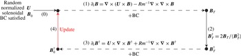
The iterative optimization process.

2.4.3. Optimization scheme
The optimization itself is an iterative procedure. As illustrated in figure 1, we initialize the algorithm with random solenoidal and normalized
 $\boldsymbol{U}$
and
 $\boldsymbol{B}_{0}$
that satisfy the boundary conditions (step
 $(0)$
). Each iteration in the optimization loop is decomposed in four steps. The magnetic field is time-stepped from time 0 to time
 $T$
, satisfying the induction equation, Gauss’ law and the boundary conditions (step
 $(1)$
). Knowing
 $\boldsymbol{B}_{T}$
, one initializes
 $\boldsymbol{B}_{T}^{\dagger }$
using the compatibility equation (2.8) (step
 $(2)$
). The adjoint (2.9) is integrated backwards from time
 $T$
to time
 $0$
, such that
 $\boldsymbol{B}^{\dagger }$
remains solenoidal and the boundary conditions are satisfied (step
 $(3)$
). This results in knowledge of
 $\boldsymbol{B}_{0}^{\dagger }$
, which is needed to evaluate
 ${\it\delta}\mathscr{L}/{\it\delta}\boldsymbol{B}_{0}$
. The time integral
 $\int _{0}^{T}\boldsymbol{B}\times (\boldsymbol{{\rm\nabla}}\times \boldsymbol{B}^{\dagger })\,\text{d}t$
that appears in
 ${\it\delta}\mathscr{L}/{\it\delta}\boldsymbol{U}$
is calculated using Simpson’s composite quadrature rule, which demands the knowledge of
 $\boldsymbol{B}$
and
 $\boldsymbol{B}^{\dagger }$
at all times; this can cause excessive memory demands and is avoided by using a checkpoint strategy, see Willis (Reference Willis2012). We are then ready to propose better estimates for
 $\boldsymbol{U}$
and
 $\boldsymbol{B}_{0}$
(step (4)). We precondition using a diagonal approximation to the Hessian of the form
 $$\begin{eqnarray}\displaystyle \widehat{\frac{{\it\delta}^{2}\mathscr{L}}{{\it\delta}\boldsymbol{U}{\it\delta}\boldsymbol{U}}}(\boldsymbol{m})\approx -2{\it\lambda}_{1}{\rm\pi}^{2}m^{2},\quad \widehat{\frac{{\it\delta}^{2}\mathscr{L}}{{\it\delta}\boldsymbol{B}_{0}{\it\delta}\boldsymbol{B}_{0}}}(\boldsymbol{m})\approx -2{\it\lambda}_{2}. & & \displaystyle\end{eqnarray}$$
We denote
 $\boldsymbol{m}=(m_{x},m_{y},m_{z})$
and
 $m^{2}=(m_{x}^{2}+m_{y}^{2}+m_{z}^{2})$
. This allows us to write updates as
 $$\begin{eqnarray}\displaystyle & \displaystyle \widehat{\boldsymbol{U}}(\boldsymbol{m}):=\widehat{\boldsymbol{U}}(\boldsymbol{m})+\frac{{\it\Delta}_{1}}{2{\it\lambda}_{1}{\rm\pi}^{2}m^{2}}\widehat{\frac{{\it\delta}\mathscr{L}}{{\it\delta}\boldsymbol{U}}}(\boldsymbol{m}), & \displaystyle\end{eqnarray}$$
 $$\begin{eqnarray}\displaystyle & \displaystyle \widehat{\boldsymbol{B}}_{0}(\boldsymbol{m}):=\widehat{\boldsymbol{B}}_{0}(\boldsymbol{m})+\frac{{\it\Delta}_{2}}{2{\it\lambda}_{2}}\widehat{\frac{{\it\delta}\mathscr{L}}{{\it\delta}\boldsymbol{B}_{0}}}(\boldsymbol{m}); & \displaystyle\end{eqnarray}$$
 ${\it\Delta}_{1}\in [0,1]$
and
 ${\it\Delta}_{2}\in [0,1]$
to prevent large steps in wrong directions, following precisely the same method as Pringle et al. (Reference Pringle, Willis and Kerswell2012).
The update cannot be evaluated as long as values of
 ${\it\Pi}_{1}$
,
 ${\it\Pi}_{2}$
,
 ${\it\lambda}_{1}$
,
 ${\it\lambda}_{2}$
are not set. Interestingly, they are exactly determined by requiring that the updated fields still satisfy the constraints. The values of
 ${\it\Pi}_{1}$
and
 ${\it\Pi}_{2}$
are set by requiring that the updated fields
 $\boldsymbol{U}$
,
 $\boldsymbol{B}_{0}$
remain solenoidal;
 ${\it\lambda}_{1},{\it\lambda}_{2}$
are fixed by the requirement that the updated
 $\boldsymbol{U}$
and
 $\boldsymbol{B}_{0}$
remain normalized.
After the update, the forward branch of the loop can be relaunched and the entire process iterated as many times as necessary. We measure progress in the optimization through
 $$\begin{eqnarray}\displaystyle r_{i}=\sqrt{\left\langle \left(\frac{{\it\delta}\mathscr{ L}}{{\it\delta}\boldsymbol{U}}\right)_{i}^{2}+\left(\frac{{\it\delta}\mathscr{L}}{{\it\delta}\boldsymbol{B}_{\mathbf{0}}}\right)_{i}^{2}\right\rangle }, & & \displaystyle\end{eqnarray}$$
where
 $i=1,2,\ldots$
is the iteration number. In essence, we need
 $\lim _{i\rightarrow +\infty }r_{i}=0$
for convergence, but in numerical simulations it is not easy to determine a threshold value for
 $r_{i}$
beneath which we can call an optimization sufficiently converged.
We note finally that the optimizer can get stuck in local minima if they exist, and for this reason, it is important to repeat optimizations with different and independent initial random fields. We will perform a perturbation study around the identified optima.
2.4.4. Testing
As a first test of our code we reproduce Willis’ results. In the absence of all projectors, using periodic flows, we reproduce the minimal magnetic
 $Rm$
for dynamo action under the enstrophy norm for a periodic flow in a cube as
 $Rm_{c,min}=2.48{\rm\pi}^{2}$
. The extra factor of
 ${\rm\pi}^{2}$
results from the use of a different length scale in the definition (2.2) of
 $Rm$
(our periodic box has size 2, Willis’ box has size
 $2{\rm\pi}$
). It should be noted that for a unit box with periodic boundaries, Willis’ result becomes
 $Rm_{c,min}=9.92{\rm\pi}^{2}$
; we shall need this reference value in our comparisons of § 3.3.
The projectors used to restrict the fields to particular classes only appear in a few places in the code: at initialization of the random fields and after each update. They have been tested in a separate manner and we are confident that these minimal modifications are correct.
3. Results
All results presented in this section have been obtained using a strict protocol. We initialize
 $\boldsymbol{U}$
,
 $\boldsymbol{B}_{0}$
with normally distributed random spectral coefficients, project out the non-solenoidal part, restrict the functions to the specified classes and normalize the fields properly. We solve direct and adjoint induction equations with
 $32^{3}$
resolution for NNT- and NTT-type boundary conditions and
 $48^{3}$
for NNN and TTT.
The question arises of how to set the terminal time
 $T$
. To be sure of dynamo action we want this to be several magnetic decay times, and we choose this to be four decay times. The decay time in a size
 $L$
box for the magnetic field with all four types of boundary conditions cannot be larger than
 $$\begin{eqnarray}\displaystyle t_{decay}=\frac{L^{2}}{{\it\eta}{\rm\pi}^{2}}. & & \displaystyle\end{eqnarray}$$
Our time scale is measured in units of
 $S^{-1}$
, and thus we convert this time into these units. This leads to a non-dimensional time horizon
 $T=4Rm/{\rm\pi}^{2}$
when the box is of size unity. Our computations confirm that this is long enough to get past the transient growth stage and allows for a reasonably short computational time (
 ${\leqslant}$
5 min for one iteration). We call an optimization ‘converged’ after
 $i$
iterations, if the residue
 $r_{i}\lesssim 10^{-3}$
.
3.1. Illustrating the iterative optimization in progress
We fix
 $Rm=7.80{\rm\pi}^{2}$
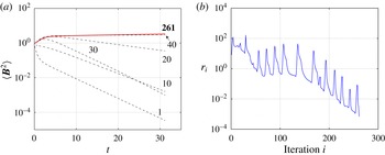
and implement NNT boundary conditions for the magnetic field. Figure 2(a) displays
 $\langle \boldsymbol{B}^{2}\rangle$
as a function of time
 $t$
, as the optimization makes progress. The initial random fields cannot support a dynamo at iteration 1, and we see exponential decay at late times. As we iterate the optimization loop, the final magnetic energy gradually increases, such that at iteration 261 it is very slightly growing with time but essentially no longer changing as the iterations proceed. This converged optimal is a slightly supercritical dynamo, because we show in § 3.2 that the minimal dynamo threshold
 $Rm=Rm_{c,min}=7.52{\rm\pi}^{2}$
for NNT boundary conditions.
Figure 2(b) shows the corresponding error measure
 $r_{i}$
as a function of iteration number
 $i$
. From the start until the end, this error goes down by five orders of magnitude, which indicates the success of the optimization. The erratic path on the descent is the result of the way in which
 ${\it\Delta}_{1}$
and
 ${\it\Delta}_{2}$
are varied. This may perhaps be avoided, but we did not find better ways than Pringle et al. (Reference Pringle, Willis and Kerswell2012) to increase the speed of convergence.
An illustration of the iterative optimization procedure. Magnetic fields with imposed NNT boundary conditions are considered,
 $Rm=7.80{\rm\pi}^{2}$
; (a) for different values of the iteration, the magnetic energy as a function of time; (b) the non-dimensional residue
 $r_{i}$
(2.24) as a function of iteration
 $i$
.

3.2. Growth rates
 ${\it\gamma}$
of optimized dynamos as a function of
$Rm$


In a more systematic survey, we vary
 $Rm$
in significant intervals. For each value of
 $Rm$
, five independent optimizations are launched from different random seeds. We measure the asymptotic growth rates
 ${\it\gamma}$
of the optimized dynamos at late times
 $t$
, where
 $$\begin{eqnarray}\displaystyle \langle \boldsymbol{B}(\boldsymbol{x},t)^{2}\rangle \sim \text{e}^{2{\it\gamma}t}. & & \displaystyle\end{eqnarray}$$
In practice, we measure the growth rate in the following way. We integrate the induction equation using the optimal
 $\boldsymbol{U}$
and the initial
 $\boldsymbol{B}_{0}$
over an extended time horizon to
 $T=12Rm/{\rm\pi}^{2}$
. The energy growth rate
 ${\it\gamma}$
is measured during the last diffusive time interval, where we are always far away from the initial transient. In figure 2(a), the growth rate of the magnetic energy in the final iteration is
 ${\it\gamma}=0.005$
using this definition.
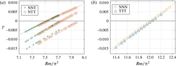
In figure 3, we group the optimal growth rates
 ${\it\gamma}$
obtained from these independent optimizations as a function of
 $Rm$
and for the four types of boundary conditions. Figure 3(a) shows cases NNT and NTT. We immediately recognize that both types of boundary conditions lead to very similar optimal growth rates. We also recognize the existence of three distinct lines. The line furthest to the left defines the real optimal branch, but some runs did converge towards suboptimal branches. Figure 3(b) shows cases NNN and TTT. Here also, both types of boundary conditions lead to very similar optimal growth rates, but we only have one optimal line.
Growth rates of optimized dynamos as a function of
 $Rm$
and for different magnetic boundary conditions; (a) NNT and NTT boundaries; (b) NNN and TTT boundaries.

3.3. Minimal dynamo thresholds
$Rm_{c,min}$

An important quantity in this study is
 $Rm_{c,min}$
, the minimal critical magnetic Reynolds number. Within the specified class of flows, no flow will act as a dynamo when
 $Rm<Rm_{c,min}$
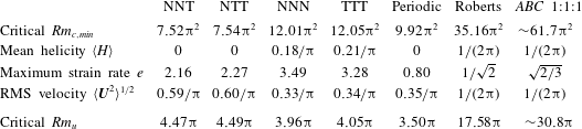
. We measure these lower bounds for dynamo action by performing a linear regression on the optimal growth rates of figure 3, which allows us to identify
 $Rm_{c,min}$
where
 ${\it\gamma}=0$
. The results are given in the first row of table 1. The mixed boundary conditions (NNT, NTT) allow for a lower
 $Rm_{c,min}$
than with perfectly conducting or pseudovacuum boundary conditions (TTT, NNN).
Some properties of the optimal flows, together with some other flows of interest. The first four columns have given magnetic boundary conditions (NNT, etc.) whereas the next three have periodic magnetic boundary conditions. The r.m.s. (root mean square) vorticity is set to unity. The periodic flow is the optimal reported in Willis (Reference Willis2012), rescaled to a unit box; the Roberts flow is an ABC flow with
 $A=B=1,C=0$
. The ABC flow 1:1:1 has all coefficients equal. The critical
 $Rm_{u}$
is the minimal threshold for dynamo action with unity kinetic energy as defined in (4.1). For our optimal flows, they are calculated from the r.m.s. velocity and from
 $Rm=Rm_{c,min}$
as in (4.3).

In the same table 1, we have added some reference values for critical dynamo thresholds. Willis’ (Reference Willis2012) periodic optimal dynamo has a larger threshold than our mixed boundary optimal. We can also compare with thresholds for Roberts (Reference Roberts1972) and ABC flows. Using the fact that for these flows the enstrophy and r.m.s. velocity are equal to unity in a
 $2{\rm\pi}$
box, we can find the values of
 $Rm_{u}$
from published values: for Roberts the value 8.79 (note [17] of Willis (Reference Willis2012) and figure 4 of Alexakis (Reference Alexakis2011) for a supercritical value of 10) is adjusted by a factor of
 $2{\rm\pi}$
to scale to a unit cube; for ABC 1:1:1 we adjust the classic value of 8.9 (Arnold & Korkina Reference Arnold and Korkina1983; Galloway & Frisch Reference Galloway and Frisch1984; Bouya & Dormy Reference Bouya and Dormy2013) by a factor of
 $\sqrt{3}$
to give unit r.m.s. velocity in a
 $2{\rm\pi}$
box and then scale to the unit cube. We find that these published values of
 $Rm$
are 4–7 times above our lower bounds.
3.4. Spatial profiles and kinetic energy spectra
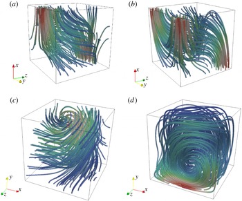
The spatial profiles of the velocity field at the minimal threshold
 $Rm_{c,min}$
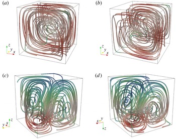
are represented by streamlines in figure 4. Lines are coloured by intensity and initialized at random locations. In all cases, we see that the flow is properly confined to the cube as dictated by our boundary conditions.
Velocity field streamlines of the optimal flow at the minimal critical magnetic Reynolds number
 $Rm_{c,min}$
and for different magnetic boundary conditions: (a) NNT optimal flow; (b) NNT optimal flow; (c) NNN optimal flow; (d) TTT optimal flow.

In the flows for the NNT and NTT optima, we see one major vortex (figure 4
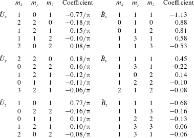
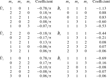
a,b). Both velocity fields also seem to be quite correlated, and this will be measured more precisely subsequently. In tables 2 and 3, we give the first five dominant modes for the optimal flow and the final magnetic field for the NNT and NTT optima. We find that
 $95\,\%$
of the enstrophy and
 ${>}89\,\%$
of the final magnetic energy are contained in these five modes. Moreover, the first two dominant modes in the optimal flow (NNT,
 $83\,\%$
of the enstrophy; NTT,
 $86\,\%$
of the enstrophy) can be written as
 $\boldsymbol{U}=\boldsymbol{{\rm\nabla}}\times \boldsymbol{A}$
, where
 $\boldsymbol{A}$
is
 $$\begin{eqnarray}\displaystyle \text{NNT}:\quad \left[\begin{array}{@{}c@{}}A_{x}(x,y,z)\\ A_{y}(x,y,z)\\ A_{z}(x,y,z)\end{array}\right]=\left[\begin{array}{@{}cc@{}}0.16 & \displaystyle \frac{1}{(2{\rm\pi})^{2}}\sin (2{\rm\pi}y)\sin (2{\rm\pi}z)\\ 0.77 & \displaystyle \frac{1}{{\rm\pi}^{2}}\sin ({\rm\pi}x)\sin ({\rm\pi}z)\\ -0.18 & \displaystyle \frac{1}{(2{\rm\pi})^{2}}\sin (2{\rm\pi}x)\sin (2{\rm\pi}y)\end{array}\right]; & & \displaystyle\end{eqnarray}$$
 $$\begin{eqnarray}\displaystyle \text{NTT}:\quad \left[\begin{array}{@{}c@{}}A_{x}(x,y,z)\\ A_{y}(x,y,z)\\ A_{z}(x,y,z)\end{array}\right]=\left[\begin{array}{@{}cc@{}}-0.17 & \displaystyle \frac{1}{(2{\rm\pi})^{2}}\sin (2{\rm\pi}y)\sin (2{\rm\pi}z)\\ 0.78 & \displaystyle \frac{1}{{\rm\pi}^{2}}\sin ({\rm\pi}x)\sin ({\rm\pi}z)\\ 0.18 & \displaystyle \frac{1}{(2{\rm\pi})^{2}}\sin (2{\rm\pi}x)\sin (2{\rm\pi}y)\end{array}\right]. & & \displaystyle\end{eqnarray}$$
 $Rm_{c}$
corresponding to the reduced optimal flow with two dominant modes is
 $9.58{\rm\pi}^{2}$
for NNT type and
 $9.38{\rm\pi}^{2}$
for NTT type.
In the flows for the NNN and TTT optima, we see three vortices (figure 4 c,d) and again a significant correlation if one rotates the profiles properly. However, this pair cannot be easily described by a few dominant modes. Both the flows and the final magnetic fields for the NNN and TTT optima have higher percentage contributions from small scales than the NNT and NTT pair.
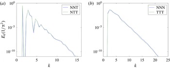
One-dimensional kinetic energy spectra for optimal dynamos at the threshold
 $Rm_{c,min}$
: (a) NNT and NTT spectra; (b) NNN and TTT spectra.

For NNT, the first five dominant modes of the optimal velocity field and the final magnetic field, accounting for
 $95\,\%$
of the enstrophy and
 $90\,\%$
of the final magnetic energy.

For NTT, the first five dominant modes of the optimal velocity field and the final magnetic field, accounting for
 $95\,\%$
of the enstrophy and
 $89\,\%$
of the final magnetic energy.

The spectral content of a flow field is often characterized using the one-dimensional kinetic energy spectrum. We calculate the one-dimensional kinetic energy spectra
 $E(k)$
, where
 $k=|\boldsymbol{m}|$
, and show them in figure 5. The energy density decreases steeply and exponentially, which is an indication of spectral spatial convergence. Decreasing several orders of magnitude from
 $k\simeq 1$
to
 $k\simeq 12{-}16$
, we clearly have a spatially resolved calculation. Numerical errors due to the finite grid spacing are consequently expected to be small.
Late-time magnetic field eigenmodes are shown in figure 6. We see the signature of the different magnetic boundary conditions in each of the plots, but magnetic field eigenmodes are no longer correlated by pairs. We see S-shaped structures in the mixed boundary cases and spiralling structures in both the NNN and TTT cases.
Magnetic field streamlines of the optimal solution at the critical magnetic Reynolds number
 $Rm_{c,min}$
at time
 $T=12$
diffusion time units: (a) NNT optimal magnetic field mode; (b) NTT optimal magnetic field mode; (c) NNN optimal magnetic field mode; (d) TTT optimal magnetic field mode.

3.5. Perturbation study
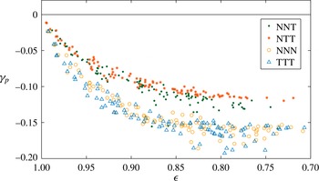
Due to the large-scale nature of the optimization and the fact that we can only launch a small number of independent optimizations, one might fear that the optima are perhaps only local optima. Such local optima can indeed exist and even have an important basin of attraction in parameter space (we observed them in figure 3 a). To ensure the robustness of our results, we perform a perturbation study on the identified optima at the minimal dynamo thresholds.
Perturbation study: the optimal dynamo flows at threshold are perturbed by random flows. We show dynamo growth rates
 ${\it\gamma}_{p}$
found with these perturbed flows as a function of the correlation amplitude. None of the points are above the optimal value
 ${\it\gamma}=0$
, and as the correlation amplitude goes up, we see that the effect of the perturbations decreases.

To do so, we generate a normally distributed random perturbation flow with variable amplitude. We add this perturbation flow to the optimal velocity field at
 $Rm_{c,min}$
and renormalize so as to have a unit enstrophy in the perturbed flow, denoted
 $\boldsymbol{U}_{p}$
. We then integrate the induction equation with this new flow
 $\boldsymbol{U}_{p}$
while keeping
 $\boldsymbol{B}_{0}$
unchanged and measure late-time growth rates
 ${\it\gamma}_{p}$
. We define a correlation amplitude
 $$\begin{eqnarray}\displaystyle {\it\epsilon}=\frac{\langle \boldsymbol{U}_{p}\boldsymbol{\cdot }\boldsymbol{U}_{o}\rangle }{\langle \boldsymbol{U}_{p}^{2}\rangle ^{1/2}\langle \boldsymbol{U}_{o}^{2}\rangle ^{1/2}} & & \displaystyle\end{eqnarray}$$
to measure by how far the new velocity field
 $\boldsymbol{U}_{p}$
differs from the unperturbed optimal field
 $\boldsymbol{U}_{o}$
. This process is repeated using 400 different perturbations of various amplitudes, and each of these runs adds a point to the plot of figure 7, which shows the perturbed growth rate
 ${\it\gamma}_{p}$
as a function of the correlation amplitude
 ${\it\epsilon}$
. None of the perturbations allow us to find growth rates
 ${\it\gamma}_{p}$
larger than
 $0$
, which is an indication that our optima are correctly calculated.
4. Analysis and discussion
4.1. Helicity
The helicity
 $H=\boldsymbol{U}\boldsymbol{\cdot }(\boldsymbol{{\rm\nabla}}\times \boldsymbol{U})$
is a popular quantity in dynamo theory which measures the alignment of the flow and its vorticity. Several laminar dynamos such as Ponomarenko flow, Roberts flow and ABC flow are helical and satisfy the Beltrami property
 $\boldsymbol{{\rm\nabla}}\times \boldsymbol{U}\sim \boldsymbol{U}$
, but helicity also plays a prominent role in mean-field dynamo theory (Moffatt Reference Moffatt1978). How helical are our optimal dynamos?
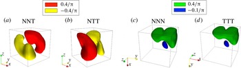
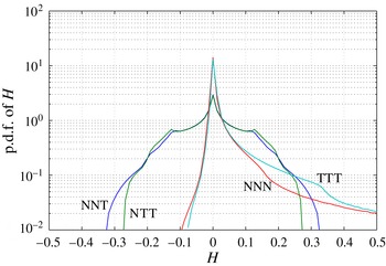
In figure 8, we show some isosurfaces of helicity of the optimal flows at threshold for the four types of magnetic boundary conditions. In the mixed boundary cases NNT and NTT, we see two symmetrical lobes of helicity. This symmetry is lost in the cases of TTT and NNN. Figure 9 shows probability density functions (p.d.f.s) of the helicity. We observe a strong pairwise correlation as before. In all set-ups NNT, NTT, NNN, TTT, the value
 $H=0$
is the most probable within the cube. Cases NNT and NTT are similar and the p.d.f.s are symmetrical, implying that the helicity is zero on average. This is not the case with NNN and TTT; these optima have a preferentially positive helicity. Mean helicities are reported in table 1 and remain well below unity.
Helicity isosurface of amplitude: (a,b)
 $-0.4/{\rm\pi}$
(yellow) and
 $0.4/{\rm\pi}$
(red) for NNT and NTT optimal flow; (c,d)
 $-0.1/{\rm\pi}$
(blue) and
 $0.4/{\rm\pi}$
(green) for NNN and TTT optimal flow.

Probability density function of helicity in the box for the different optimal flows at criticality,
 $Rm_{min,c}$
.

4.2. Minimal magnetic Reynolds number based on r.m.s. velocity
The magnetic Reynolds number (2.2) we used in this work is not very standard in the dynamo literature. We needed to use this definition since it is compatible with the enstrophy normalization which was necessary because optimizations with normalized kinetic energy do not yield converged optima. A more standard definition for the magnetic Reynolds number is based on the r.m.s. velocity
 $U$
:
 $$\begin{eqnarray}\displaystyle Rm_{u}=\frac{UL}{{\it\eta}}. & & \displaystyle\end{eqnarray}$$
We can calculate this
 $Rm_{u}$
a posteriori, since we can measure
 $$\begin{eqnarray}\displaystyle \frac{U}{SL}=\langle \boldsymbol{U}^{2}\rangle ^{1/2} & & \displaystyle\end{eqnarray}$$
from the optima. In this way, we have
 $$\begin{eqnarray}\displaystyle Rm_{u}=Rm\langle \boldsymbol{U}^{2}\rangle ^{1/2}, & & \displaystyle\end{eqnarray}$$
which yields the values reported in table 1. Interestingly, it seems that with this definition of
 $Rm_{u}$
we can reinterpret the results. The NNN and TTT optima have now the lowest critical thresholds, before the mixed boundary condition optima NNT and TTT.
4.3. Symmetry of the cube and its consequences
To study symmetries in the flows and equations, we shift the coordinate system to the centre of the cube (but do not change notation to avoid unnecessary complexity). In this frame, the cubical boundary surface is the union of coordinate surfaces
 $x=\pm 1/2$
,
 $y=\pm 1/2$
,
 $z=\pm 1/2$
. This boundary is clearly mapped onto itself, by any possible permutation of
 $x,y,z$
combined with any possible change of sign. More explicitly, with
 $\boldsymbol{x}=(x,y,z)$
, a cube is symmetrical with respect to all operations
 $\unicode[STIX]{x1D64D}\boldsymbol{x}$
:
 $$\begin{eqnarray}\displaystyle \left.\begin{array}{@{}ll@{}}\unicode[STIX]{x1D64D}\boldsymbol{x}=(s_{1}x,s_{2}y,s_{3}z), & \unicode[STIX]{x1D64D}\boldsymbol{x}=(s_{2}y,s_{1}x,s_{3}z),\\ \unicode[STIX]{x1D64D}\boldsymbol{x}=(s_{2}y,s_{3}z,s_{1}x), & \unicode[STIX]{x1D64D}\boldsymbol{x}=(s_{3}z,s_{2}y,s_{1}x),\\ \unicode[STIX]{x1D64D}\boldsymbol{x}=(s_{3}z,s_{1}x,s_{2}y), & \unicode[STIX]{x1D64D}\boldsymbol{x}=(s_{1}x,s_{3}z,s_{2}y),\end{array}\!\!\right\} & & \displaystyle\end{eqnarray}$$
with
 $s_{1},s_{2},s_{3}=\pm 1$
. This parametrizes the 48-member symmetry group of the cube (or octahedral)
 $O_{h}$
. Next to the trivial identity, each transform can be associated with a rotation or a reflection with respect to a mirror plane. Operators
 $\unicode[STIX]{x1D64D}$
can be represented using orthogonal matrices
 $\unicode[STIX]{x1D64D}$
(
 $\unicode[STIX]{x1D64D}^{-1}=\unicode[STIX]{x1D64D}^{\text{T}}$
).
We study the presence and the consequences of these symmetries in the optimized dynamo problem. The symmetries explain why optima are degenerate and why we find exactly the same optimal growth rates in pairs (NNT and NTT, NNN and TTT).
4.3.1. Trivial consequence of symmetry: degeneracy of the optima
The equations of the kinematic dynamo problem are invariant under any coordinate transform
 $\boldsymbol{x}=\unicode[STIX]{x1D64D}^{\text{T}}\widetilde{\boldsymbol{x}},\widetilde{\boldsymbol{x}}=\unicode[STIX]{x1D64D}\boldsymbol{x}$
that involves
 $\unicode[STIX]{x1D64D}$
, an orthogonal matrix:
 $$\begin{eqnarray}\displaystyle \left.\begin{array}{@{}c@{}}\partial _{t}\boldsymbol{B}=\boldsymbol{{\rm\nabla}}\times (\boldsymbol{U}\times \boldsymbol{B})+Rm^{-1}{\rm\nabla}^{2}\boldsymbol{B}\quad \Leftrightarrow \quad \partial _{t}\widetilde{\boldsymbol{B}}=\widetilde{\boldsymbol{{\rm\nabla}}}\times (\widetilde{\boldsymbol{U}}\times \widetilde{\boldsymbol{B}})+Rm^{-1}\widetilde{{\rm\nabla}}^{2}\widetilde{\boldsymbol{B}},\\ \boldsymbol{{\rm\nabla}}\boldsymbol{\cdot }\boldsymbol{B}=0\quad \Leftrightarrow \quad \widetilde{\boldsymbol{{\rm\nabla}}}\boldsymbol{\cdot }\widetilde{\boldsymbol{B}}=0.\end{array}\!\!\right\} & & \displaystyle\end{eqnarray}$$
Here, the two fields are related as
 $$\begin{eqnarray}\displaystyle \boldsymbol{U}(\boldsymbol{x})=\unicode[STIX]{x1D64D}^{\text{T}}\widetilde{\boldsymbol{U}}(\unicode[STIX]{x1D64D}\boldsymbol{x}),\quad \boldsymbol{B}(\boldsymbol{x})=\unicode[STIX]{x1D64D}^{\text{T}}\widetilde{\boldsymbol{B}}(\unicode[STIX]{x1D64D}\boldsymbol{x}). & & \displaystyle\end{eqnarray}$$
An immediate consequence in the present context of optimized dynamo action is that if the boundary conditions are also invariant under
 $\unicode[STIX]{x1D64D}$
transformation, we can say that
 $$\begin{eqnarray}\displaystyle \boldsymbol{U}(\boldsymbol{x})\text{ is an optimal dynamo}\quad \Leftrightarrow \quad \unicode[STIX]{x1D64D}^{\text{T}}\boldsymbol{U}(\mathscr{\unicode[STIX]{x1D64D}\boldsymbol{x}})\text{ is an optimal dynamo}. & & \displaystyle\end{eqnarray}$$
In the cases of NNN and TTT, we have the same types of boundary conditions everywhere, which implies that the NNN and TTT optima are both 48-fold degenerate. The mixed boundaries NNT and NTT have symmetry groups that are reduced to dihedral symmetry:
 $$\begin{eqnarray}\displaystyle \underbrace{\begin{array}{@{}c@{}}\unicode[STIX]{x1D64D}\boldsymbol{x}=(s_{1}x,s_{2}y,s_{3}z),\\ \unicode[STIX]{x1D64D}\boldsymbol{x}=(s_{2}y,s_{1}x,s_{3}z),\end{array}}_{\text{NNT}}\quad \underbrace{\begin{array}{@{}c@{}}\unicode[STIX]{x1D64D}\boldsymbol{x}=(s_{1}x,s_{2}y,s_{3}z),\\ \unicode[STIX]{x1D64D}\boldsymbol{x}=(s_{1}x,s_{3}z,s_{2}y),\end{array}}_{\text{NTT}} & & \displaystyle\end{eqnarray}$$
with
 $s_{1},s_{2},s_{3}=\pm 1$
and thus only 16 members. As a result, NNT and NTT optima are 16-fold degenerate. The fact that we observe
 $3=48/16$
separate ‘optimality’ branches in the mixed boundary case (see figure 3
a) is probably also related to this reduced symmetry group of the boundaries.
In the simulations, we do see this trivial degeneracy: depending on the random initialization, the optimizer converges to optima that have the same optimal growth rates, but with rotated or mirror reflected spatial structures.
4.3.2. Symmetry and anti-correlation in the optimal flows
Instead of investigating the symmetry of the equations and boundary conditions, we can also measure whether the optimal solutions themselves are symmetric. Let us introduce some notations and concepts. Two vector field
 $\boldsymbol{V}_{1}(\boldsymbol{x})$
and
 $\boldsymbol{V}_{2}(\boldsymbol{x})$
are correlated
 $(+)$
or anti-correlated
 $(-)$
by an isometry
 $\unicode[STIX]{x1D64D}$
when
 $$\begin{eqnarray}\displaystyle \unicode[STIX]{x1D64D}^{\text{T}}\boldsymbol{V}_{1}(\unicode[STIX]{x1D64D}\boldsymbol{x})=\pm \boldsymbol{V}_{2}(\boldsymbol{x}). & & \displaystyle\end{eqnarray}$$
Choosing
 $\boldsymbol{V}_{1}=\boldsymbol{V}_{2}=\boldsymbol{V}$
, we can check whether the vector field
 $\boldsymbol{V}$
is symmetrical
 $(+)$
or anti-symmetrical
 $(-)$
with respect to some
 $\unicode[STIX]{x1D64D}$
. Let us denote
 $\boldsymbol{V}_{i,\unicode[STIX]{x1D64D}}=\unicode[STIX]{x1D64D}^{\text{T}}\boldsymbol{V}_{i}(\unicode[STIX]{x1D64D}\boldsymbol{x})$
and
 $$\begin{eqnarray}\displaystyle s_{ij}=\frac{\langle \boldsymbol{V}_{i,\unicode[STIX]{x1D64D}}\boldsymbol{\cdot }\boldsymbol{V}_{j}\rangle }{\langle \boldsymbol{V}_{i,\unicode[STIX]{x1D64D}}^{2}\rangle ^{1/2}\langle \boldsymbol{V}_{j}^{2}\rangle ^{1/2}}, & & \displaystyle\end{eqnarray}$$
with
 $i,j=1,2$
. Using this quantity we can study the (anti)-correlations and (anti)-symmetries of the different optimal flows in a systematic way and with respect to all 48 isometries
 $\unicode[STIX]{x1D64D}$
of the cube.
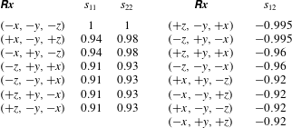
For NNT and NTT optimal flows,
 $\boldsymbol{V}_{1}=\boldsymbol{U}_{\text{NNT}}$
and
 $\boldsymbol{V}_{2}=\boldsymbol{U}_{\text{NTT}}$
, we have found several high scores
 $|s_{ij}|>0.9$
, which are listed in table 4. The first row on the left-hand side of the table shows that these optimal flows are inversion symmetric:
 $$\begin{eqnarray}\displaystyle \boldsymbol{U}_{\text{NNT}}(\boldsymbol{x})=-\boldsymbol{U}_{\text{NNT}}(-\boldsymbol{x}),\quad \boldsymbol{U}_{\text{NTT}}(\boldsymbol{x})=-\boldsymbol{U}_{\text{NTT}}(-\boldsymbol{x}). & & \displaystyle\end{eqnarray}$$
This immediately explains why these flows have no mean helicity. The other isometries are not exact, but the scores are still high enough to say that there is a significant correlation. On the right-hand side of the table, we see that the optimal flows
 $\boldsymbol{U}_{\text{NNT}}$
and
 $\boldsymbol{U}_{\text{NTT}}$
are almost perfectly anti-correlated by an isometry. The most negative score
 $\min (s_{12})=-0.995$
is found for the operation
 $\unicode[STIX]{x1D64D}\boldsymbol{x}=(z,-y,x)$
and its inverse. This corresponds to a rotation of
 ${\rm\pi}$
about the axis
 $(\boldsymbol{e}_{x}+\boldsymbol{e}_{z})/\sqrt{2}$
and a reflection with respect to a plane with that vector as unit normal. Up to
 $0.5\,\%$
we can say that
 $$\begin{eqnarray}\displaystyle \boldsymbol{U}_{\text{NTT}}(\boldsymbol{x})\simeq -\unicode[STIX]{x1D64D}^{\text{T}}\boldsymbol{U}_{\text{NNT}}(\unicode[STIX]{x1D64D}\boldsymbol{x}). & & \displaystyle\end{eqnarray}$$
When applied to the boundary, the transform
 $\unicode[STIX]{x1D64D}\boldsymbol{x}=(z,-y,x)$
essentially maps the NNT boundary into a TNN boundary, which is the exact complementary of an NTT boundary, under the exchange
 $\text{N}\leftrightarrow \text{T}$
. As explained below, this anti-correlation explains why NNT optima and NTT optima have the same growth rates.
For NNN and TTT optimal flows,
 $\boldsymbol{V}_{1}=\boldsymbol{U}_{\text{NNN}}$
and
 $\boldsymbol{V}_{2}=\boldsymbol{U}_{\text{TTT}}$
, we find maximal correlations,
 $\max |s_{11}|=0.42$
for NNN,
 $\max |s_{22}|=0.61$
for TTT. This is not significant: all symmetries are broken in NNN and TTT optimal flows, in agreement with figure 4(c,d). We do find an almost perfect anti-correlation between the different optima:
 $\min (s_{12})=-0.97$
, for a single isometry
 $\unicode[STIX]{x1D64D}\boldsymbol{x}=(y,x,-z)$
. Up to
 $3\,\%$
we can say that
 $$\begin{eqnarray}\displaystyle \boldsymbol{U}_{\text{NNN}}(\boldsymbol{x})\simeq -\unicode[STIX]{x1D64D}^{\text{T}}\boldsymbol{U}_{\text{TTT}}(\unicode[STIX]{x1D64D}\boldsymbol{x}). & & \displaystyle\end{eqnarray}$$
The transform
 $\unicode[STIX]{x1D64D}\boldsymbol{x}=(y,x,-z)$
corresponds to a rotation of
 ${\rm\pi}$
around the vector
 $(\boldsymbol{e}_{x}+\boldsymbol{e}_{y})/\sqrt{2}$
.
Symmetries and anti-correlations of optimal flows
 $\boldsymbol{V}_{1}=\boldsymbol{U}_{\text{NNT}}$
,
 $\boldsymbol{V}_{2}=\boldsymbol{U}_{\text{NTT}}$
under isometries of the cube (see (4.10) for the definition of
 $s_{ij}$
).

Considering the degeneracy of the optima, the perfect anti-correlation of the optimal flows can be simplified to
 $$\begin{eqnarray}\displaystyle \left.\begin{array}{@{}c@{}}\boldsymbol{U}_{\text{NNT}}\text{ is optimal for NNT}\quad \Leftrightarrow \quad -\boldsymbol{U}_{\text{NNT}}\text{ is optimal for TTN},\\ \boldsymbol{U}_{\text{NNN}}\text{ is optimal for NNN}\quad \Leftrightarrow \quad -\boldsymbol{U}_{\text{NNN}}\text{ is optimal for TTT},\end{array}\!\!\right\} & & \displaystyle\end{eqnarray}$$
which will serve as a starting point for the next section.
4.3.3. Identical growth rates for complementary boundary conditions
In recent work, Favier & Proctor (Reference Favier and Proctor2013) have shown that for a general fluid domain
 $\mathscr{V}$
with impermeable walls, a stationary dynamo
 $\boldsymbol{U}$
that is anti-symmetric with respect to an isometry
 $\unicode[STIX]{x1D64D}$
of the system,
 $$\begin{eqnarray}\displaystyle \boldsymbol{U}(\boldsymbol{x})=-\unicode[STIX]{x1D64D}^{-1}\boldsymbol{U}(\unicode[STIX]{x1D64D}\boldsymbol{x}), & & \displaystyle\end{eqnarray}$$
will grow magnetic fields with the exact same growth rate
 ${\it\gamma}$
for both the types of complementary pseudovacuum (N) or perfectly conducting (T) boundaries.
In the present context, none of our optimal flows are anti-symmetric with respect to themselves, but we do find the same growth rates
 ${\it\gamma}$
and also find pairwise anti-correlation for the optimal flows of complementary set-ups (NNT and NTT, NNN and TTT). We can explain this using the same type of argument as developed by Favier & Proctor (Reference Favier and Proctor2013), and limit the demonstration here to the case of NNN and TTT.
Suppose an arbitrary fluid volume
 $\mathscr{V}$
, with perfectly conducting T boundaries. A flow
 $\boldsymbol{U}_{\text{T}}$
drives a magnetic field eigenmode
 $\boldsymbol{b}_{\text{T}}(\boldsymbol{x})\exp ({\it\gamma}t)$
, which means that
 $$\begin{eqnarray}\displaystyle {\it\gamma}\boldsymbol{b}_{\text{T}}-\boldsymbol{{\rm\nabla}}\times (\boldsymbol{U}_{\text{T}}\times \boldsymbol{b}_{\text{T}})+Rm^{-1}\boldsymbol{{\rm\nabla}}\times \boldsymbol{{\rm\nabla}}\times \boldsymbol{b}_{\text{T}}=0. & & \displaystyle\end{eqnarray}$$
We suppose that
 ${\it\gamma}$
is real. On the boundary,
 $$\begin{eqnarray}\displaystyle \boldsymbol{U}_{\text{T}}\boldsymbol{\cdot }\boldsymbol{n}|_{{\it\Sigma}}=0,\quad \boldsymbol{n}\times \boldsymbol{e}_{\text{T}}|_{{\it\Sigma}}=0, & & \displaystyle\end{eqnarray}$$
where
 $\boldsymbol{e}_{\text{T}}=Rm^{-1}\boldsymbol{{\rm\nabla}}\times \boldsymbol{b}_{\text{T}}-\boldsymbol{U}_{\text{T}}\times \boldsymbol{b}_{\text{T}}$
is the electrical field. We now manipulate this equation by taking the scalar product of (4.16) with
 $\boldsymbol{a}_{\text{T}}$
and integrating over the volume. Partial integration brings us to
 $$\begin{eqnarray}\displaystyle & & \displaystyle \langle ({\it\gamma}\boldsymbol{a}_{\text{T}}+\boldsymbol{U}_{\text{T}}\times (\boldsymbol{{\rm\nabla}}\times \boldsymbol{a}_{\text{T}})+Rm^{-1}\boldsymbol{{\rm\nabla}}\times \boldsymbol{{\rm\nabla}}\times \boldsymbol{a}_{\text{T}})\boldsymbol{\cdot }\boldsymbol{b}_{\text{T}}\rangle \nonumber\\ \displaystyle & & \displaystyle \quad +\,\underbrace{\oint _{{\it\Sigma}}(\boldsymbol{e}_{\text{T}}\times \boldsymbol{n})\boldsymbol{\cdot }\boldsymbol{a}_{\text{T}}\,\text{d}S}_{=0}+\,Rm^{-1}\oint _{{\it\Sigma}}((\boldsymbol{{\rm\nabla}}\times \boldsymbol{a}_{\text{T}})\times \boldsymbol{n})\boldsymbol{\cdot }\boldsymbol{b}_{\text{T}}\,\text{d}S=0.\end{eqnarray}$$
The first boundary term disappears because of the boundary condition on
 $\boldsymbol{e}_{\text{T}}$
. A sufficient condition to get
 $0$
on both sides is
 $$\begin{eqnarray}\displaystyle & \displaystyle {\it\gamma}\boldsymbol{a}_{\text{T}}+\boldsymbol{U}_{\text{T}}\times (\boldsymbol{{\rm\nabla}}\times \boldsymbol{a}_{\text{T}})+Rm^{-1}\boldsymbol{{\rm\nabla}}\times \boldsymbol{{\rm\nabla}}\times \boldsymbol{a}_{\text{T}}=0 & \displaystyle\end{eqnarray}$$
 $$\begin{eqnarray}\displaystyle & \displaystyle +\text{BC}\boldsymbol{ : }(\boldsymbol{{\rm\nabla}}\times \boldsymbol{a}_{\text{T}})\times \boldsymbol{n}|_{{\it\Sigma}}=0. & \displaystyle\end{eqnarray}$$
 $\text{BC}$
, the field
 $\boldsymbol{b}_{\text{N}}=\boldsymbol{{\rm\nabla}}\times \boldsymbol{a}_{\text{T}}$
is normal to the boundaries. By taking the curl of (4.19), we find that this field
 $\boldsymbol{b}_{\text{N}}$
solves
 $$\begin{eqnarray}\displaystyle & \displaystyle {\it\gamma}\boldsymbol{b}_{\text{N}}=\boldsymbol{{\rm\nabla}}\times [(-\boldsymbol{U}_{\text{T}})\times \boldsymbol{b}_{\text{N}}]-Rm^{-1}\boldsymbol{{\rm\nabla}}\times \boldsymbol{{\rm\nabla}}\times \boldsymbol{b}_{\text{N}} & \displaystyle\end{eqnarray}$$
 $$\begin{eqnarray}\displaystyle & \displaystyle +\text{BC}\boldsymbol{ : }\boldsymbol{b}_{\text{N}}\times \boldsymbol{n}|_{{\it\Sigma}}=0. & \displaystyle\end{eqnarray}$$
 $\boldsymbol{U}_{\text{N}}=-\boldsymbol{U}_{\text{T}}$
is equally a dynamo for a magnetic field eigenmode that will be normal to the boundaries and it will grow at exactly the same rate
 ${\it\gamma}$
.
4.4. Backus bound
Backus (Reference Backus1958) took a different definition for the magnetic Reynolds number
 $Rm_{B}$
in terms of the maximum strain rate of the flow. With the present scaling, we have
 $Rm_{B}=S_{max}L^{2}/{\it\eta}=\unicode[STIX]{x1D65A}Rm$
, where
 $\unicode[STIX]{x1D65A}=S_{max}/S$
is the maximum eigenvalue of the non-dimensional strain rate tensor with components
 $$\begin{eqnarray}\displaystyle \unicode[STIX]{x1D626}_{ij}={\textstyle \frac{1}{2}}(\partial _{i}U_{j}+\partial _{j}U_{i}). & & \displaystyle\end{eqnarray}$$
We calculated this maximal local strain
 $\unicode[STIX]{x1D65A}$
for our optimal flows at threshold, and show values in table 1. We note that the NNN and TTT optimal flows display a considerably larger maximal strain than the NNT and NTT optima or the periodic box case of Willis (Reference Willis2012).
The Backus bound provides a minimal requirement on
 $Rm_{B}$
based on the energy equation of
 $\boldsymbol{B}$
. A necessary condition for dynamo action is (see also Proctor Reference Proctor1977)
 $$\begin{eqnarray}\displaystyle Rm_{B}\geqslant \min \underbrace{\displaystyle \frac{\displaystyle \int _{\mathcal{V}_{1}}|\boldsymbol{{\rm\nabla}}\times \boldsymbol{B}|^{2}\,\text{d}\mathscr{V}}{\displaystyle \int _{\mathcal{V}_{2}}|\boldsymbol{B}|^{2}\,\text{d}\mathscr{V}}}_{{\it\beta}}. & & \displaystyle\end{eqnarray}$$
In this formula,
 $\mathscr{V}_{1}$
is the fluid domain and
 $\mathscr{V}_{2}$
is the entire domain, but here
 $\mathscr{V}_{1}=\mathscr{V}_{2}$
. The largest-scale magnetic fields within the fluid domain supply a lower bound on
 ${\it\beta}$
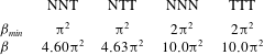
. The measured
 ${\it\beta}$
for the optimal set of modes is expected to be larger, since the structure of the magnetic field is not entirely large scale.
Comparison of
 ${\it\beta}_{min}$
and the measured
 ${\it\beta}$
for the final magnetic field
 $\boldsymbol{B}_{T}$
at
 $Rm_{c,min}$
.

Our best dynamo, with
 $e=2.16$
and
 $Rm_{c,min}=7.52{\rm\pi}^{2}$
, from table 1, then has
 $Rm_{B}=16.2{\rm\pi}^{2}$
, approximately 16 times larger than the Backus bound
 ${\it\beta}_{min}$
. This indicates that the maximum strain rate is significantly larger than the strain developed in most of the volume, and we know from table 5 that the
 ${\it\beta}$
realized is
 ${\sim}5$
times the minimal available value. This explains the observed difference.
5. Conclusion
By adapting the procedure of Willis (Reference Willis2012), we have developed a Cartesian model to find the most efficient dynamo with a flow confined within a cube. Table 1 shows the values of
 $Rm_{c,min}$
for our results and for the original results of Willis (Reference Willis2012) along with thresholds for some famous ABC flows. We have been careful to refer all results to the same size of box. Compared with the ABC flows, our optimal dynamos have thresholds that are approximately a factor of 5 to 8 lower. On comparing with the optimal of Willis (Reference Willis2012), also using normalized enstrophy, it transpires that periodic magnetic boundary conditions are not the optimal boundary conditions to enable efficiency. One can see this heuristically by considering the smallest-size magnetic structures that are allowed by the box and its boundary conditions. Periodic boundary conditions necessarily only allow a field with one full wavelength within the box, whereas our boundary conditions allow a half wavelength (see e.g. (2.14)). Thus, it is possible to have lower dissipation and a more efficient dynamo.
The symmetries of the cube are responsible for a strong degeneracy of the optima. A more surprising consequence of symmetry is that we find that when
 $\boldsymbol{U}$
generates an optimal dynamo for a given set of idealized boundary conditions, then
 $-\boldsymbol{U}$
can generate an optimal dynamo too, but for a different and complementary set of boundary conditions. We explain this observation using a similar argument to the one developed by Favier & Proctor (Reference Favier and Proctor2013).
Compared with existing results on lower bounds, we showed in § 4.4 that our best dynamo operates approximately 16 times above the Backus bound. We can conjecture what this implies for spherical dynamos with insulating boundary conditions, although rigorous results must follow from calculations. This observed minimum bound for
 $Rm_{B}$
of
 ${\sim}16.2{\rm\pi}^{2}$
suggests that working dynamos might need to have
 $Rm_{B}\sim 150$
in practice when based on the maximum strain rate. We finally note that our optimal flows tend not to be very helical, a result already seen by Willis.
The next challenge is to develop the same strategy for the sphere. The sphere has more applications in laboratory settings and also represents a simpler geometry; one can conjecture that it will operate with a lower magnetic Reynolds number as a result of this simpler geometry. We hope to report on this topic in the future.
Acknowledgements
This work was supported by the ETH Research Commission through grant ETH-08 13-2 for which we are grateful. A.J. is partially supported by ERC grant 247303 ‘MFECE’. We thank A. Willis for his interest and advice on several aspects of the work, and M. Proctor for useful discussions. W.H. thanks Y. Duguet for introducing him to the topic.
Appendix A. Projectors in spectral space
In our numerical method, we use a periodic box code. All fields or field components are represented on the standard Fourier basis adapted to a periodic cube of size 2. A function
 $f(x,y,z)$
then has the expansion
 $$\begin{eqnarray}\displaystyle f(x,y,z)=\mathop{\sum }_{m_{x},m_{y},m_{z}\in \mathbb{Z}}\widetilde{f}(m_{x},m_{y},m_{z})\text{e}^{\text{i}{\rm\pi}(m_{x}x+m_{y}y+m_{z}z)}. & & \displaystyle\end{eqnarray}$$
Let
 $\mathscr{E}$
be the space of all periodic functions on the cube with size 2. We then have
 $$\begin{eqnarray}\displaystyle \mathscr{E}=\mathscr{E}_{ccc}\oplus \mathscr{E}_{ccs}\oplus \mathscr{E}_{csc}\oplus \mathscr{E}_{scc}\oplus \mathscr{E}_{ssc}\oplus \mathscr{E}_{scs}\oplus \mathscr{E}_{css}\oplus \mathscr{E}_{sss}, & & \displaystyle\end{eqnarray}$$
which is easily understood by rewriting the generic Fourier expansion using Euler’s rule. That same rule also allows us to find projectors
 $\mathscr{P}_{ccc},\mathscr{P}_{ccs},\ldots ,\mathscr{P}_{sss}$
that allow us to restrict a function
 $f(x,y,z)$
to the required class. For example, for all
 $f\in \mathscr{E}$
,
 $$\begin{eqnarray}\displaystyle \mathscr{P}_{ccc}f\in \mathscr{E}_{ccc},\mathscr{P}_{ccs}f\in \mathscr{E}_{ccs},\ldots ,\mathscr{P}_{sss}f\in \mathscr{E}_{sss}. & & \displaystyle\end{eqnarray}$$
These projectors are most easily defined in spectral space. Given the Fourier-space coefficients
 $\tilde{f}(m_{x},m_{y},m_{z})$
and denoting Fourier-space amplitudes
 $\tilde{f}(\pm m_{x},\pm m_{y},\pm m_{z})$
as
 $\tilde{f}_{\pm \pm \pm }$
, we find that
 $$\begin{eqnarray}\displaystyle \left.\begin{array}{@{}c@{}}\widetilde{\mathscr{P}_{ccc}f}_{+++}={\textstyle \frac{1}{4}}Re(\,\tilde{f}_{+++}+\tilde{f}_{+-+}+\tilde{f}_{++-}+\tilde{f}_{+--}),\\ \widetilde{\mathscr{P}_{ssc}f}_{+++}={\textstyle \frac{1}{4}}Re(\,\tilde{f}_{+++}-\tilde{f}_{+-+}+\tilde{f}_{++-}-\tilde{f}_{+--}),\\ \widetilde{\mathscr{P}_{scs}f}_{+++}={\textstyle \frac{1}{4}}Re(\,\tilde{f}_{+++}+\tilde{f}_{+-+}-\tilde{f}_{++-}-\tilde{f}_{+--}),\\ \widetilde{\mathscr{P}_{css}f}_{+++}={\textstyle \frac{1}{4}}Re(\,\tilde{f}_{+++}-\tilde{f}_{+-+}-\tilde{f}_{++-}+\tilde{f}_{+--})\end{array}\!\!\right\} & & \displaystyle\end{eqnarray}$$
and
 $$\begin{eqnarray}\displaystyle \left.\begin{array}{@{}c@{}}\displaystyle \widetilde{\mathscr{P}_{scc}f}_{+++}=\frac{\text{i}}{4}\text{Im}[\tilde{f}_{+++}+\tilde{f}_{+-+}+\tilde{f}_{++-}+\tilde{f}_{+--}],\\ \displaystyle \widetilde{\mathscr{P}_{csc}f}_{+++}=\frac{\text{i}}{4}\text{Im}[\tilde{f}_{+++}-\tilde{f}_{+-+}+\tilde{f}_{++-}-\tilde{f}_{+--}],\\ \displaystyle \widetilde{\mathscr{P}_{ccs}f}_{+++}=\frac{\text{i}}{4}\text{Im}[\tilde{f}_{+++}+\tilde{f}_{+-+}-\tilde{f}_{++-}-\tilde{f}_{+--}],\\ \displaystyle \widetilde{\mathscr{P}_{sss}f}_{+++}=\frac{\text{i}}{4}\text{Im}[\tilde{f}_{+++}-\tilde{f}_{+-+}-\tilde{f}_{++-}+\tilde{f}_{+--}]\end{array}\!\!\right\} & & \displaystyle\end{eqnarray}$$
for all values of
 $m_{x},m_{y},m_{z}\in \mathbb{Z}$
. If numerical resources are not a problem, these projectors can be used to transform a periodic box code into one that sets idealized boundary conditions on the walls of a cube with half that size. Otherwise, it is strongly advised to make dedicated codes using sine and cosine transforms.