




1 Introduction
It is well known that the motion of a compressible fluid of uniform property has two well-known fundamental processes, revealed by applying the Helmholtz decomposition to the momentum equation, namely taking its curl and divergence: the vector transversal process (VTP) characterized by the vorticity  $\unicode[STIX]{x1D74E}=\unicode[STIX]{x1D735}\times \boldsymbol{u}$,
 $\boldsymbol{u}$ being the velocity, and the scalar longitudinal process (SLP) characterized kinematically by dilatation
 $\unicode[STIX]{x1D717}=\unicode[STIX]{x1D735}\boldsymbol{\cdot }\boldsymbol{u}$ and dynamically by other scalars such as the pressure
 $p$, the density
 $\unicode[STIX]{x1D70C}$, the enthalpy
 $h$, the temperature
 $T$ and the entropy
 $s$, etc. In a viscous complex flow, including coexistence and strong interactions of shear layers, concentrated vortices, sound waves, shocks and entropy variation, as well as their interactions with a solid boundary, the two processes are coupled both inside the fluid due to nonlinearity and at the boundary of the flow due to the no-slip condition. The physical sources of each process are contained in these couplings, of which the identification is of crucial importance in practical flow management. For reviews of the existing theories and some applications of process splitting and coupling, see e.g. Wu, Ma & Zhou (Reference Wu, Ma and Zhou2015) and Wu, Liu & Liu (Reference Wu, Liu and Liu2018). Of course, this complex-flow diagnosis tool can by no means replace computational and experimental fluid dynamics (CFD and EFD) that can resolve increasingly complicated gas flows and turbulence. Rather, its role can be fully exhibited only when high-quality flow-field data from CFD/EFD are available, to explain in detail the physics behind the evolution of these structures, and their mutual generation/modulation.
The general theory for VTP is nothing but the vorticity and vortex dynamics. Its foundation has been well established, including the nonlinear evolution, production at the boundary and inside the fluid of the vorticity field due to its self-nonlinearity and couplings with SLP, so that it has become a powerful diagnosis tool in the study of turbulent coherent structures. In contrast, however, a well-structured systematic theory for SLP is still lacking. To orient our goals, below we first briefly review the existing relevant theories and some of their difficulties.
1.1 The development and difficulties of longitudinal-process theories
Modern development of SLP theory grew from the classic gas dynamics (e.g. Courant & Friedrichs Reference Courant and Friedrichs1948; Liepmann & Roshko Reference Liepmann and Roshko1957; Emmons Reference Emmons1958), which laid down a firm basis for high-speed aerodynamics. But since there the main body of the flow is assumed to be inviscid and irrotational, as well as mostly steady, this classic theory can only be applied to simple attached flow.
The theory for splitting a linearized Navier–Stokes (NS) flow into VTP and SLP was pioneered by Lagerstrom, Cole & Trilling (Reference Lagerstrom, Cole and Trilling1949), with heat conduction being added by Wu (Reference Wu1956). Along this direction, Kovásznay (Reference Kovásznay1953) calls the VTP the vorticity mode, and proposed that the SLP consists of a sound mode and an entropy mode due to their different governing equations, as seen by the dispersion relations of the linearized NS equations (e.g. Pierce Reference Pierce1981; Tam, Webb & Dong Reference Tam, Webb and Dong1993). Mao, Shi & Wu (Reference Mao, Shi and Wu2010) further proved that, for a small disturbance to an unbounded fluid otherwise at rest, the linearized equation for the three modes can be fully decoupled. The linearized triple-mode decomposition was generalized to nonlinear viscous gas flow by Chu & Kovásznay (Reference Chu and Kovásznay1958) in an iterative perturbation formulation, where the differential operators remain to be linearized.
Since the entropy mode shown below is quite simple, one focus on SLP is the theory of sound mode, for which two approaches have been developed first with different subjects and objectives, although they partly overlap. One focus is on the acoustics in moving inhomogeneous media (AMIM) pioneered by Blokhintzev (Reference Blokhintzev1946) with many following studies as documented by Ostashev (Reference Ostashev1997). Another is on the famous acoustic analogy theory initiated by Lighthill (Reference Lighthill1952) aimed at predicting noise production and propagation in a turbulent jet. The latter signified the birth of modern aeroacoustics (e.g. Goldstein Reference Goldstein1976) and, combined with CFD, has led to an active field of computational aeroacoustics (e.g. Wang, Freund & Lele Reference Wang, Freund and Lele2006). Then, another significant advance of SLP in the 1950s came also from Lighthill (Reference Lighthill, Batchelor and Davies1956), a unified theory of the nonlinear evolution and annihilation of a finite-amplitude sound wave in viscous and heat-conducting flow, including the formation of shock layers. When the Reynolds number of the flow is high, diffusion and heat conduction are significant only in shocks (Lighthill Reference Lighthill, Batchelor and Davies1956) and the linearized far field (Mao et al. Reference Mao, Shi and Wu2010; Liu Reference Liu2018).
The above theoretical advances, although all in the same field of SLP and partly overlapping, have been considered different branches with respective subjects and objectives (e.g. Ostashev Reference Ostashev1997). The acoustic analogy is not mentioned in the book of Whitham (Reference Whitham1974) and only briefly touched upon in Lighthill (Reference Lighthill1978). These advances, if put together, are still insufficient to form a unified SLP theory as a competitive counterpart to vorticity dynamics for VTP due to their inherent limitations. Difficulties appeared mostly with the sound mode. On the one hand, the precise identification of the physical source of sound has never been well addressed in either AMIM or aeroacoustics. In the former, the main concern is the sound propagation in complex moving media rather than its physical production, while in the latter, which should address the sound production by fluid motion, the issue has remained a longstanding controversial problem (e.g. Ffowcs Williams Reference Ffowcs Williams1977; Jordan & Gervais Reference Jordan and Gervais2008). One of the key issues involved here is the alternative choice of time-rate operators, the Eulerian operator  $\unicode[STIX]{x2202}/\unicode[STIX]{x2202}t$ (the
 $\unicode[STIX]{x2202}_{t}$-form for short) versus the Lagrangian operator
 $D/Dt$ (the
 $D$-form for short). While in AMIM one usually uses the
 $D$-form, in the acoustic analogy the
 $\unicode[STIX]{x2202}_{t}$-form is the orthodox approach, until Phillips (Reference Phillips1960) turned to the
 $D$-form with ‘a reluctant abandonment of the acoustic analogy’, followed by the well-known work of Lilley (Reference Lilley1974), among the others.
On the other hand, Lighthill’s theory on viscous and finite-amplitude sound waves was analytically developed, because only one-dimensional plane waves as a function of  $(x,t)$ are considered. Its extension to higher dimensions within the potential-flow framework is called nonlinear acoustics (e.g. Enflo & Hedberg Reference Enflo and Hedberg2002). But neither of these permits the coupling with VTP in real complex compressible vortical flows, although the vorticity has been found to be a major source of noise in turbulence.
In view of these limitations and difficulties with existing theories, Mao et al. (Reference Mao, Shi, Xuan, Su and Wu2011) initiated a study of fully nonlinear and viscous equations for the sound mode. Specifically, owing to the perfect kinematic correspondence between vorticity and dilatation, they left the conventional thermodynamic-variable formulation and derived for the first time the governing equations of dilatation  $\unicode[STIX]{x1D717}$ for the sound mode, expressed with both
 $D$-form and
 $\unicode[STIX]{x2202}_{t}$-form. They also demonstrated the consistency of these equations with and relevance to various existing SLP theories in aforementioned fields. But the identification of SLP sources remained an open issue.
1.2 The approach and main findings of this study
The present paper is a direct continuation of Mao et al. (Reference Mao, Shi, Xuan, Su and Wu2011). The basic and main findings of this paper are as follows.
Firstly, we argue that a clear source identification for the sound mode can be sorted out by observing the causality relationship inherent in various dynamic equations relevant to SLP. The physical cause of a process or variable, which can produce that process or variable from nothing as the effect, should be identified as the source. For a moving fluid, this causality naturally requires using a nonlinear operator  $D$ rather than
 $\unicode[STIX]{x2202}_{t}$; while for waves propagating on that fluid, it naturally favours the advective hyperbolic (AH) wave operator
 $D^{2}-c^{2}\unicode[STIX]{x1D6FB}^{2}$ rather than
 $\unicode[STIX]{x2202}_{t}^{2}-c^{2}\unicode[STIX]{x1D6FB}^{2}$, with
 $c$ being the wave speed relative to the fluid.
Secondly, we confine ourselves to working on real physical quantities and do not introduce auxiliary variables such as the velocity potential and vector streamfunction. Then, the formulations of SLP dynamics can be made at two levels. The first level has been widely analysed, which works on the thermodynamic variables  $p,\unicode[STIX]{x1D70C},T,s,$ etc. For the sound mode, each variable is governed by an AH wave equation. Their source terms can be clearly identified and are neat. The multiple-formulation issue has its roots in the combination of the continuity equation and thermodynamic relations. In contrast, at the second level that is our main concern, one works on a single kinematic variable, the dilatation
 $\unicode[STIX]{x1D717}$. Its governing AH wave equation for viscous and heat-conducting flows, obtained by Mao et al. (Reference Mao, Shi, Xuan, Su and Wu2011) by raising the order of
 $D$ by one, is improved here and thoroughly explored. The order raising of
 $D$ produces rich nonlinear couplings among the vorticity mode, entropy mode, sound mode as well as a purely universal kinematic mechanism (see below) not seen at the first level. These couplings affect the AH wave operator and bring in various sources for viscous and heat-conducting flow, indicating that the practical value of the AH wave equation for
 $\unicode[STIX]{x1D717}$ is its guidance in pinpointing the leading-order SLP sources in complex flows.
Thirdly, at both levels we follow the approach in fine-scale turbulence studies, to extend the vector momentum equation for  $D\boldsymbol{u}$ to an equation for
 $D\unicode[STIX]{x1D63C}$, where
 $\unicode[STIX]{x1D63C}\equiv \unicode[STIX]{x1D735}\boldsymbol{u}$ is the velocity gradient tensor, see, e.g. Meneveau (Reference Meneveau2011) and Wilczek & Meneveau (Reference Wilczek and Meneveau2014) for incompressible flow, and Wang & Lu (Reference Wang and Lu2012) and Chu & Lu (Reference Chu and Lu2013) for compressible flow, as well as references cited therein. This approach is not only neat in algebra but also opens a wider view for understanding the SLP: it is the processes solely derived from the trace of
 $\unicode[STIX]{x1D63C}$. In particular, SLP has a universal source
 $\text{tr}(\unicode[STIX]{x1D63C}^{2})(=\unicode[STIX]{x1D735}\unicode[STIX]{x1D63C}\boldsymbol{ : }\unicode[STIX]{x1D735}\unicode[STIX]{x1D63C})$, which is outside the three modes but inherent in the kinematic nonlinearity of
 $\unicode[STIX]{x1D63C}$. Then, we find that tensor
 $\unicode[STIX]{x1D63C}$ and its traces can be replaced by the surface deformation tensor
 $\unicode[STIX]{x1D63D}(=\unicode[STIX]{x1D717}\unicode[STIX]{x1D644}-\unicode[STIX]{x1D63C}^{\text{T}})$ and its traces, respectively, where
 $\unicode[STIX]{x1D644}$ is the unit tensor and the superscript
 $\text{T}$ denotes transpose. Unlike
 $\unicode[STIX]{x1D63C}$ that covers wide kinematic mechanisms,
 $\unicode[STIX]{x1D63D}$ has a single meaning as an elementary kinematic mechanism, such that the source in terms of the invariants of
 $\unicode[STIX]{x1D63D}$ is a concentrated representative compared to that of
 $\unicode[STIX]{x1D63C}$.
Finally, as a sharp scalpel, the basic concept of process splitting and couplings will be implemented throughout our entire study. The results of this study will be tested and exemplified by a low Mach flow with interaction of two co-rotating Gaussian vortices and a complex hypersonic flow with type IV shock/shock interactions.
1.3 The contents of this paper
This paper is organized as follows. As preparation, § 2 reviews the  $D$-form fundamental equations of compressible viscous flow, including using the dynamic tensor equation for
 $\unicode[STIX]{x1D63C}(=\unicode[STIX]{x1D735}\boldsymbol{u})$. A causality loop is thereby identified to distinguish the cause and effect in each equation, which is the basis of identifying the physical sources of sound mode. As comparison, the evolution equation for vorticity responsible for VTP and the anti-symmetric contraction of the
 $\unicode[STIX]{x1D63C}$-equation, is briefly reviewed.
Section 3 revisits the set of AH wave equations for the sound mode at the first level. Their sources consist of a common universal kinematic source  $\text{tr}(\unicode[STIX]{x1D63C}^{2})$, which we find can be condensed to a scalar
 $\unicode[STIX]{x1D6FD}\equiv \unicode[STIX]{x1D735}\boldsymbol{\cdot }(\unicode[STIX]{x1D63D}\boldsymbol{\cdot }\boldsymbol{u})$, a pseudo-work rate done by fluid surface deformation, along with entropy sources. Of these mathematically equivalent AH wave equations, Phillips’ equation (Phillips Reference Phillips1960) for disturbance pressure turns out to be the best representation of the sound mode.
In § 4 we continue the discussions of Mao et al. (Reference Mao, Shi, Xuan, Su and Wu2011) on both  $D$- and
 $\unicode[STIX]{x2202}_{t}$-form dilatation equations, focusing on why the
 $\unicode[STIX]{x2202}_{t}$-form cannot be used to identify physical sources of
 $\unicode[STIX]{x1D717}$, and how the
 $D$-form can and what are its rich results.
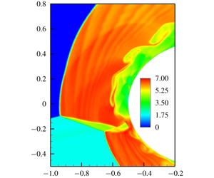
Section 5 provides two numerical examples, a low Mach flow with interaction of two co-rotating Gaussian vortices and a complex hypersonic flow with type IV shock/shock interactions, to demonstrate our theoretical findings and explain the interactions of different modes. Concluding remarks are presented in § 6, followed by two mathematical appendices.
2 Background and orientation
2.1 Fundamental equations
We consider the general motion of compressible viscous flows of a calorically perfect gas, without external addition of mass, body force and heat. By its state equation  $p=\unicode[STIX]{x1D70C}RT$, where
 $R$ is the gas constant, and the thermodynamic relation
 $$\begin{eqnarray}Tds=de+p\,d\left(\frac{1}{\unicode[STIX]{x1D70C}}\right)=dh-\frac{1}{\unicode[STIX]{x1D70C}}\,dp,\end{eqnarray}$$
where  $e$ is the internal energy, it is known that the specific entropy
 $s$ is alternatively expressible as
 $$\begin{eqnarray}\frac{ds}{c_{v}}=d(\ln p)-\unicode[STIX]{x1D6FE}\,d(\ln \unicode[STIX]{x1D70C})=d(\ln h)-(\unicode[STIX]{x1D6FE}-1)\,d(\ln \unicode[STIX]{x1D70C}),\end{eqnarray}$$
where  $\unicode[STIX]{x1D6FE}=c_{p}/c_{v}$ is the ratio of constant specific heats at constant volume and pressure. The square of the sound speed is also known as
 $$\begin{eqnarray}c^{2}=\unicode[STIX]{x1D6FE}RT=(\unicode[STIX]{x1D6FE}-1)h=\frac{\unicode[STIX]{x1D6FE}p}{\unicode[STIX]{x1D70C}}.\end{eqnarray}$$
Denoting  $D=D/Dt=\unicode[STIX]{x2202}_{t}+\boldsymbol{u}\boldsymbol{\cdot }\unicode[STIX]{x1D735}$ as the material time-rate operator, by (2.2), the continuity equation can be written in terms of thermodynamic variables
 $$\begin{eqnarray}\unicode[STIX]{x1D717}=-D(\ln \unicode[STIX]{x1D70C})=-\frac{1}{\unicode[STIX]{x1D6FE}}D(\ln p-s/c_{v})=-\frac{1}{\unicode[STIX]{x1D6FE}-1}D(\ln h-s/c_{v}),\end{eqnarray}$$
or in terms of  $c^{2}$
 $$\begin{eqnarray}c^{2}\unicode[STIX]{x1D717}=-Dh+\unicode[STIX]{x1D6FE}TDs.\end{eqnarray}$$
Then, the momentum equation is
 $$\begin{eqnarray}D\boldsymbol{u}=-\unicode[STIX]{x1D735}h+\boldsymbol{f},\quad \boldsymbol{f}\equiv T\unicode[STIX]{x1D735}s+\boldsymbol{\unicode[STIX]{x1D702}},\end{eqnarray}$$
where  $\boldsymbol{\unicode[STIX]{x1D702}}\equiv \unicode[STIX]{x1D708}_{\unicode[STIX]{x1D703}}\unicode[STIX]{x1D735}\unicode[STIX]{x1D717}-\unicode[STIX]{x1D708}\unicode[STIX]{x1D735}\times \unicode[STIX]{x1D74E}$ is the viscous force, with
 $\unicode[STIX]{x1D708}_{\unicode[STIX]{x1D703}}=(\unicode[STIX]{x1D706}+2\unicode[STIX]{x1D707})/\unicode[STIX]{x1D70C}$ and
 $\unicode[STIX]{x1D708}=\unicode[STIX]{x1D707}/\unicode[STIX]{x1D70C}$ being the kinematic longitudinal and transverse viscosities, respectively. The energy balance can be expressed by the entropy equation
 $$\begin{eqnarray}\unicode[STIX]{x1D70C}TDs=\unicode[STIX]{x1D6F7}-\unicode[STIX]{x1D735}\boldsymbol{\cdot }\boldsymbol{q},\end{eqnarray}$$
where  $\unicode[STIX]{x1D6F7}$ is the dissipation function,
 $\boldsymbol{q}=-k\unicode[STIX]{x1D735}T$ is the heat flux with
 $k$ being the heat conductivity.
Throughout the theoretical development in this paper we adopt the linear diffusion approximation introduced by Lighthill (Reference Lighthill, Batchelor and Davies1956) in developing a unified analytical theory for a viscous sound wave of finite amplitude, its Riemann invariants and weak shock structure, by which  $\unicode[STIX]{x1D708},\unicode[STIX]{x1D708}_{\unicode[STIX]{x1D703}}$ and
 $k$ simply take their constant values. This is not an a priori hypothesis; rather, by careful scale analysis, Lighthill proved that, if
 $\unicode[STIX]{x1D708}f(\boldsymbol{x},t)$ is any viscous function in the above fundamental equations, then for polytropic gas and in a flow region without a strong shock the estimate
 $$\begin{eqnarray}\frac{|\unicode[STIX]{x1D708}f-\unicode[STIX]{x1D708}_{0}f|}{|\unicode[STIX]{x1D708}_{0}f|}\ll 1\end{eqnarray}$$
is indeed true, and similarly for  $\unicode[STIX]{x1D708}_{\unicode[STIX]{x1D703}}f$ or
 $kf$. Of course this approximation is invalid when
 $\unicode[STIX]{x1D707}$ strongly depends on
 $T$; but in our study shock layers are mainly resolved by CFD, see § 5. There, the above fundamental equations formulated by the
 $D$ operator have been transformed into conservative form, along with temperature-dependent variable
 $\unicode[STIX]{x1D708}(T)$. Moreover, while the linear diffusion approximation does not require
 $\unicode[STIX]{x1D708}$ itself to be small, our main concern is nevertheless advection-dominated flows at large Reynolds numbers, of which a formal introduction is of course the non-dimensionalization of the above equations as shown by, e.g. Lagerstrom (Reference Lagerstrom and Moore1964) (pp. 151–153). Here, we continue using dimensional notations for neatness, but whenever we talk about a large Reynolds number or small viscosity we shall say that in dimensionless form the viscous effect is of
 $O(\unicode[STIX]{x1D716})$ with
 $\unicode[STIX]{x1D716}=Re^{-1}\ll 1$.
Finally, as mentioned in § 1, we extend (2.6) to a tensor form in terms of the velocity-gradient tensor  $\unicode[STIX]{x1D735}\boldsymbol{u}=\unicode[STIX]{x1D63C}$, of which the time evolution following fluid particles is given by the gradient of (2.6),
 $$\begin{eqnarray}D\unicode[STIX]{x1D63C}+\unicode[STIX]{x1D63C}^{2}=-\boldsymbol{H}_{h}+\unicode[STIX]{x1D735}\boldsymbol{f},\end{eqnarray}$$
where  $\boldsymbol{H}_{h}\equiv \unicode[STIX]{x1D735}\unicode[STIX]{x1D735}h$ is the Hessian of enthalpy. Like the pressure Hessian
 $\unicode[STIX]{x1D735}\unicode[STIX]{x1D735}p(\equiv \boldsymbol{H}_{p})$ for incompressible flow,
 $\boldsymbol{H}_{h}$ is expected to be responsible for non-local interactions in compressible flow.
2.2 Causality mechanisms in governing equations
As said in § 1, the choices of characteristic variables of SLP along with their governing equations and sources are not unique. This situation underscores the crucial importance of identifying the causal relationship among different variables and nonlinear terms in the relevant equations. In so doing, we may well focus on an inviscid flow model first. Then, the cause and effect in an equation of the type  $DF=G$, say, can be easily identified, since integrating this equation following a fluid particle with respect to
 $t$ can surely update
 $F$ as the effect, with
 $G$ being the cause. Equations (2.4), (2.6) or (2.9), and (2.7) are all of this type. For example, consider a solid body that starts to move at
 $t=0$ in a fluid otherwise at rest. Owing to the fluidity, the fluid yields to the body by generating an
 $\unicode[STIX]{x1D63C}$ field kinematically, including its isotropic part
 $\unicode[STIX]{x1D717}$. Then, by (2.4), a fluid particle will gain disturbances of
 $\unicode[STIX]{x1D70C},p$ and
 $h$ isentropically at
 $t>0$ from none. In turn, these generated variables will cause a dynamic change of
 $\unicode[STIX]{x1D63C}$ by (2.9) along with a newly created
 $\unicode[STIX]{x1D717}$-field. Therefore, the kinematic–kinetic processes governed by (2.4) and (2.9) make the causality chain a closed loop. Obviously, the loop may also start from a given initial field of
 $(\unicode[STIX]{x1D70C},p,h)$ that produces the
 $(\unicode[STIX]{x1D63C},\unicode[STIX]{x1D717})$-field by (2.9), and ends with a newly produced field of
 $(\unicode[STIX]{x1D70C},p,h)$ via (2.4). In any case, this loop repeats as time goes on and creates the rich world of flows. Evidently, for sound propagation relative to a non-uniformly moving fluid, we have another type of equation, say
 $(D^{2}-c^{2}\unicode[STIX]{x1D6FB}^{2})P=Q$, for which the causality is also easily identified.
Viscous and heat-conducting effects appear in real flows, which cause the entropy production and also affect the evolution of  $\unicode[STIX]{x1D63C}$, especially in the shock region and the long-time evolution problem. But these effects do not alter the basic cause-and-effect identification inferred for inviscid flow. By gas kinetic theory, they occur during molecular drifting to new positions from one equilibrium
 $(p,\unicode[STIX]{x1D70C})$ state to another, and hence slightly lag behind (Lighthill Reference Lighthill, Batchelor and Davies1956).
2.3 On the source identification for scalar longitudinal process
The above cause-and-effect identification provides an objective basis for defining the physical source of SLP in the interior of the fluid. In this regard, the entropy mode governed by (2.7) is free from any ambiguity; Serrin (Reference Serrin, Flugge and Truesdell1959) has clearly explained why  $\unicode[STIX]{x1D6F7}-\unicode[STIX]{x1D735}\boldsymbol{\cdot }\boldsymbol{q}$ is the true physical source by the original entropy definition
 $\text{d}s=\text{d}Q/T$. Thus, we focus on the sound mode below and just make a couple of remarks on the entropy mode in § 3.2. In general, for different evolution equations involving more than one variable, their nonlinear terms can be classified into three types as defined by Mao et al. (Reference Mao, Shi, Xuan, Su and Wu2011): the self-nonlinearity; the cross-modulation by which a variable modifies another that already exists; the source that can produce a variable from none as time goes on. Therefore, we use the word ‘source’ as the synonym of a cause in the causality chain of a process. It will be seen that, although the choice of the characteristic sound-mode variables and their governing equations can vary, and hence the sources of SLP may take varying forms, they are just different faces of the same physical origin that can well be identified.
It should be stressed, however, that this source identification still has only limited clarity. Although ideally the source of a specific mode should be fully independent of the characteristic variables of this mode, in practice, one can rarely achieve such a pure goal due to the following reasons.
Firstly, the source identification depends on the specific theoretical mode splitting, which itself can hardly be ideally ‘clean’. For example, across a curved shock one says that the baroclinic effect  $\unicode[STIX]{x1D735}T\times \unicode[STIX]{x1D735}s$ is a source of vorticity (see the next subsection), but ignores the reaction of the newly generated vorticity field to the shock – it may be too weak or its analysis hardly feasible. In other words, in the study of vorticity evolution one does not consider the influence of the vorticity field on the temperature or entropy, which are assumed known from the thermodynamic process.
Secondly, in certain fields of the sound mode such as aeroacoustics, the flow field often needs to be further decomposed into a weak acoustic fluctuations generated and propagated in the mean flow field although the mean flow also contains SLP. Some nonlinear terms would be further split into a linearized propagation term and a Reynolds-stress-like source term for the fluctuation equation. But in this paper we are confined to the SLP behaviour of the whole flow without making such a distinction. Consequently, the general results of source identification to be presented below may differ from those in aeroacoustics.
Thirdly, yet very importantly, an ideally thorough longitudinal–transverse splitting requires a decomposition of velocity  $\boldsymbol{u}$
 $$\begin{eqnarray}\boldsymbol{u}=\unicode[STIX]{x1D735}\unicode[STIX]{x1D719}+\unicode[STIX]{x1D735}\times \unicode[STIX]{x1D74D}=\boldsymbol{u}_{\unicode[STIX]{x1D719}}+\boldsymbol{u}_{\unicode[STIX]{x1D713}},\quad \unicode[STIX]{x1D6FB}^{2}\unicode[STIX]{x1D719}=\unicode[STIX]{x1D717},\quad \unicode[STIX]{x1D6FB}^{2}\unicode[STIX]{x1D74D}=-\unicode[STIX]{x1D74E},\end{eqnarray}$$
where  $\boldsymbol{u}_{\unicode[STIX]{x1D719}}$ and
 $\boldsymbol{u}_{\unicode[STIX]{x1D713}}$ are the longitudinal and transverse parts of
 $\boldsymbol{u}$, induced non-locally by
 $\unicode[STIX]{x1D717}$ and
 $\unicode[STIX]{x1D74E}$, respectively (this non-locality has nothing to do with causality and should be distinguished from the non-local interactions implied by
 $\boldsymbol{H}_{p}$ or
 $\boldsymbol{H}_{h}$). The acceleration
 $\boldsymbol{a}=D\boldsymbol{u}$ should also be accordingly decomposed. However, if we substitute (2.10) into (2.9) and operator
 $D$, the resulting equation for
 $\unicode[STIX]{x1D719}$ will be formidably complicated as observed by Mao et al. (Reference Mao, Shi, Xuan, Su and Wu2011). Although the multi-valueness and/or singularity of
 $\unicode[STIX]{x1D719}$ and
 $\unicode[STIX]{x1D74D}$ are directly and universally responsible for the total lift and drag on a body in steady flow, they are not physically testable but merely auxiliary variables (Liu Reference Liu2018). In this paper, we only work on real physical quantities and shall take
 $\boldsymbol{u}$ and
 $\boldsymbol{a}$ as a whole, and tolerate some ambiguity in the splitting of VTP and SLP, as pointed out by Mao et al. (Reference Mao, Shi, Xuan, Su and Wu2011). For example, in the vortex-sound theory it suffices to say that
 $\unicode[STIX]{x1D735}\boldsymbol{\cdot }(\unicode[STIX]{x1D74E}\times \boldsymbol{u})$ is the source of sound without splitting of
 $\boldsymbol{u}$.
2.4 Vector transverse process or vorticity mode
To be self-containing and for comparison, we now briefly review a couple of known results for VTP. In contrast to taking the curl of (2.6) in the conventional formulation, in tensor formulation VTP follows from taking the antisymmetric part of (2.9) by its contraction with the permutation tensor  $\boldsymbol{E}=\boldsymbol{e}_{i}\boldsymbol{e}_{j}\boldsymbol{e}_{k}\unicode[STIX]{x1D716}_{ijk}$. This yields the vorticity dynamics equation
 $$\begin{eqnarray}D\unicode[STIX]{x1D74E}+(\unicode[STIX]{x1D717}\unicode[STIX]{x1D644}-\unicode[STIX]{x1D63F})\boldsymbol{\cdot }\unicode[STIX]{x1D74E}=\unicode[STIX]{x1D735}\times \boldsymbol{f}=\unicode[STIX]{x1D735}T\times \unicode[STIX]{x1D735}s+\unicode[STIX]{x1D708}\unicode[STIX]{x1D6FB}^{2}\unicode[STIX]{x1D74E},\end{eqnarray}$$
where  $\unicode[STIX]{x1D63F}$ is the strain rate tensor. This
 $D$-type equation has local
 $|\boldsymbol{u}|$ as its characteristic speed. Owing to the nonlinear term
 $\unicode[STIX]{x1D63C}^{2}$ in (2.9), the evolution of vorticity is modulated by the trace and symmetric part of
 $\unicode[STIX]{x1D63C}$,
 $(\unicode[STIX]{x1D717}\unicode[STIX]{x1D644}-\unicode[STIX]{x1D63F})$. The viscous term does not produce vorticity, but diffuses and dissipates the existing vorticity. The baroclinic term
 $\unicode[STIX]{x1D735}T\times \unicode[STIX]{x1D735}s$ is a familiar physical source of vorticity inside the flow field. In addition, although not seen from (2.11), it is well known that the vorticity is mainly and universally created at solid walls with the tangent pressure gradient thereon as the source (via the no-slip condition). This is a crucial longitudinal–transverse boundary coupling process, slightly lagging behind the establishment of the pressure distribution.
3 Longitudinal processes by thermodynamic variables
This and the next sections present our major theoretical development. We start from the contraction of (2.9) with unit tensor  $\unicode[STIX]{x1D644}$, or the divergence of (2.6), to obtain an evolution equation of SLP,
 $$\begin{eqnarray}D\unicode[STIX]{x1D717}+\text{tr}(\unicode[STIX]{x1D63C}^{2})=-\unicode[STIX]{x1D6FB}^{2}h+\unicode[STIX]{x1D735}\boldsymbol{\cdot }\boldsymbol{f},\end{eqnarray}$$
where  $\text{tr}(\unicode[STIX]{x1D63C}^{2})=u_{j,i}u_{i,j}$ is the trace of
 $\unicode[STIX]{x1D63C}^{2}$. In contrast to (2.11), (3.1) involves double longitudinal variables
 $\unicode[STIX]{x1D717}$ and
 $h$. A single-variable SLP equation follows from removing either one of them.
3.1 Sound mode in terms of thermodynamic variables
The dilatation  $\unicode[STIX]{x1D717}$ in (3.1) is related to thermodynamic variables by (2.4). Introduce dimensionless quantities describing the relative strength of disturbances of these variables, defined by
 $$\begin{eqnarray}\left.\begin{array}{@{}c@{}}\displaystyle {\mathcal{R}}\equiv \ln \left(\frac{\unicode[STIX]{x1D70C}}{\unicode[STIX]{x1D70C}_{0}}\right),\quad {\mathcal{P}}\equiv \frac{1}{\unicode[STIX]{x1D6FE}}\ln \left(\frac{p}{p_{0}}\right),\\ \displaystyle {\mathcal{H}}\equiv \frac{1}{\unicode[STIX]{x1D6FE}-1}\ln \left(\frac{h}{h_{0}}\right)=\frac{1}{\unicode[STIX]{x1D6FE}-1}\ln \left(\frac{T}{T_{0}}\right),\quad s^{\ast }\equiv \frac{s-s_{0}}{c_{p}},\end{array}\right\}\end{eqnarray}$$
such that for a small disturbance  $f^{\prime }=f-f_{0}$ with
 $|f^{\prime }|\ll \,f_{0}$ there will be
 $\ln (f/f_{0})\simeq \,f^{\prime }/f_{0}$. Then (2.2) yields
 $$\begin{eqnarray}\displaystyle ds^{\ast }=d({\mathcal{P}}-{\mathcal{R}})=(\unicode[STIX]{x1D6FE}-1)d({\mathcal{H}}-{\mathcal{P}})=\frac{\unicode[STIX]{x1D6FE}-1}{\unicode[STIX]{x1D6FE}}d({\mathcal{H}}-{\mathcal{R}}). & & \displaystyle\end{eqnarray}$$
Then, substituting (2.4), (3.2) into (3.1), and noticing that
 $$\begin{eqnarray}T\unicode[STIX]{x1D735}s=\frac{c^{2}}{\unicode[STIX]{x1D6FE}-1}\unicode[STIX]{x1D735}s^{\ast },\end{eqnarray}$$
we easily obtain a set of single-variable AH wave equations for  ${\mathcal{R}},{\mathcal{P}}$ and
 ${\mathcal{H}}$,
 $$\begin{eqnarray}\displaystyle & \displaystyle {\mathcal{W}}{\mathcal{R}}=[\text{tr}(\unicode[STIX]{x1D63C}^{2})-\unicode[STIX]{x1D708}_{\unicode[STIX]{x1D703}}\unicode[STIX]{x1D6FB}^{2}\unicode[STIX]{x1D717}]+\unicode[STIX]{x1D735}\boldsymbol{\cdot }(c^{2}\unicode[STIX]{x1D735}s^{\ast }), & \displaystyle\end{eqnarray}$$
 $$\begin{eqnarray}\displaystyle & \displaystyle {\mathcal{W}}{\mathcal{P}}=[\text{tr}(\unicode[STIX]{x1D63C}^{2})-\unicode[STIX]{x1D708}_{\unicode[STIX]{x1D703}}\unicode[STIX]{x1D6FB}^{2}\unicode[STIX]{x1D717}]+D^{2}s^{\ast }, & \displaystyle\end{eqnarray}$$
 $$\begin{eqnarray}\displaystyle & \displaystyle {\mathcal{W}}{\mathcal{H}}=[\text{tr}(\unicode[STIX]{x1D63C}^{2})-\unicode[STIX]{x1D708}_{\unicode[STIX]{x1D703}}\unicode[STIX]{x1D6FB}^{2}\unicode[STIX]{x1D717}]+\frac{\unicode[STIX]{x1D6FE}}{\unicode[STIX]{x1D6FE}-1}D^{2}s^{\ast }-\frac{1}{\unicode[STIX]{x1D6FE}-1}\unicode[STIX]{x1D735}\boldsymbol{\cdot }(c^{2}\unicode[STIX]{x1D735}s^{\ast }), & \displaystyle\end{eqnarray}$$
where
 $$\begin{eqnarray}{\mathcal{W}}f=D^{2}f-\unicode[STIX]{x1D735}\boldsymbol{\cdot }(c^{2}\unicode[STIX]{x1D735}f)\end{eqnarray}$$
is an AH wave operator for the logarithm  $f$ of any thermodynamic variable, with varying
 $c^{2}$ given by (2.3) as the characteristic speed. These are the standard and simplest nonlinear AH equations. Since in triple-mode interactions
 $s^{\ast }$ should be one independent variable, for the above equations only one is independent. In particular, equation (3.6) is just the well-known equation derived by Phillips (Reference Phillips1960) which, after separating the acoustic disturbance from the mean flow, has led to the famous Lilley (Reference Lilley1974) equation for the noise generated by a turbulent jet.
On the right-hand side of the above sound-mode equations, there are two common terms: the kinematic nonlinearity  $\text{tr}(\unicode[STIX]{x1D63C}^{2})$ that exists universally, and the viscous term
 $-\unicode[STIX]{x1D708}_{\unicode[STIX]{x1D703}}\unicode[STIX]{x1D6FB}^{2}\unicode[STIX]{x1D717}$. The latter is not a real source, since in (3.5), for example, it leads to a term
 $\unicode[STIX]{x1D708}_{\unicode[STIX]{x1D703}}\unicode[STIX]{x1D6FB}^{2}D{\mathcal{R}}$, implying that the AH wave equation for
 ${\mathcal{R}}$ is changed to a third-order advective diffusion equation. The only difference among
 ${\mathcal{R}}$,
 ${\mathcal{P}}$ and
 ${\mathcal{H}}$ comes from the entropy-related sources: the time rate of entropy production
 $D^{2}s^{\ast }$ (from continuity) and non-uniform entropy distribution
 $\unicode[STIX]{x1D735}\boldsymbol{\cdot }(c^{2}\unicode[STIX]{x1D735}s^{\ast })=(\unicode[STIX]{x1D6FE}-1)T\unicode[STIX]{x1D735}s$ (from momentum balance).
Phillips (Reference Phillips1960) remarks that for aeroacoustics problems both  $\unicode[STIX]{x1D708}_{\unicode[STIX]{x1D703}}\unicode[STIX]{x1D6FB}^{2}\unicode[STIX]{x1D717}$ and
 $D^{2}s^{\ast }$ in (3.6) can be ignored. Actually, a simple scale analysis in the near field of low Mach flow tells that, in (3.5)–(3.7) the magnitude of
 $\unicode[STIX]{x1D735}\boldsymbol{\cdot }(c^{2}\unicode[STIX]{x1D735})$ is always far larger than that of
 $D^{2}$. This is also true if
 $f=s^{\ast }$ in (3.8), despite the fact that
 $\unicode[STIX]{x1D735}\boldsymbol{\cdot }(c^{2}\unicode[STIX]{x1D735}s^{\ast })$ and
 $D^{2}s^{\ast }$ appear separately. Our numerical studies in § 5 below confirm this estimate. Therefore, although in principle (3.5) or (3.7) can play the same role as (3.6), the latter is least influenced by the entropy variation and, as Kovásznay (Reference Kovásznay1953) and Chu & Kovásznay (Reference Chu and Kovásznay1958) suggested, may serve as the primary equation for sound mode among those in terms of thermodynamic variables.
3.2 Remarks on the entropy mode
Since
 $$\begin{eqnarray}\frac{1}{T}\unicode[STIX]{x1D6FB}^{2}T=\unicode[STIX]{x1D6FB}^{2}\ln T+|\unicode[STIX]{x1D735}\ln T|^{2}=\unicode[STIX]{x1D6FB}^{2}\ln h+|\unicode[STIX]{x1D735}\ln h|^{2},\end{eqnarray}$$
equation (2.7) can be cast to a  $DF=G$ type entropy production equation for a perfect gas
 $$\begin{eqnarray}Ds^{\ast }=\frac{\unicode[STIX]{x1D6F7}}{\unicode[STIX]{x1D70C}h}+\unicode[STIX]{x1D701}(\unicode[STIX]{x1D6FB}^{2}\ln T+|\unicode[STIX]{x1D735}\ln T|^{2}),\quad \unicode[STIX]{x1D701}\equiv \frac{\unicode[STIX]{x1D708}}{Pr},\end{eqnarray}$$
with the right-hand side being the physical sources of  $s^{\ast }$ due to dissipation and heat transfer. The characteristic speed is
 $|\boldsymbol{u}|$. The linearized version of (3.9),
 $$\begin{eqnarray}\unicode[STIX]{x2202}_{t}s^{\ast }\simeq \unicode[STIX]{x1D701}\unicode[STIX]{x1D6FB}^{2}\frac{T^{\prime }}{T_{0}},\end{eqnarray}$$
was used by Kovásznay (Reference Kovásznay1953) and Chu & Kovásznay (Reference Chu and Kovásznay1958) to analyse the entropy mode. Since they use the  $(p,s)$ pair as independent thermodynamic variables, they further presented a pressure–entropy equation
 $$\begin{eqnarray}(\unicode[STIX]{x2202}_{t}-\unicode[STIX]{x1D701}\unicode[STIX]{x1D6FB}^{2})s^{\ast }\simeq (\unicode[STIX]{x1D6FE}-1)\unicode[STIX]{x1D701}\unicode[STIX]{x1D6FB}^{2}\frac{p^{\prime }}{\unicode[STIX]{x1D6FE}p_{0}}\end{eqnarray}$$
to link the sound mode and entropy mode (of course,  $p^{\prime }/(\unicode[STIX]{x1D6FE}p_{0})$ can be replaced by
 $\unicode[STIX]{x1D70C}^{\prime }/\unicode[STIX]{x1D70C}_{0}$). This implies that an AH wave of the sound mode can result in the same kind of waves in the entropy mode. Note that the structure of (3.11) has been changed from the
 $\unicode[STIX]{x2202}_{t}F=G$ type of (3.10) to a diffusion type due to the extra appearance of
 $ds^{\ast }$ in the variable transformation via (3.3).
On the Chu–Kovásznay equation (3.11), we make two remarks. First, for real high Mach number complex flows, entropy is not just passively advected as with other variables. High peaks of  $\unicode[STIX]{x1D717}^{2}$ and
 $\unicode[STIX]{x1D714}^{2}$ must appear in strong shock layers and the viscous core of strong vortices, respectively. They may cause the peaks of nonlinear dissipation
 $\unicode[STIX]{x1D6F7}$, which evolve following the motion of shocks and vortices, making the entropy evolution deviate from simple AH waves. The relative strengths of
 $\unicode[STIX]{x1D6F7}$ and
 $\unicode[STIX]{x1D701}\unicode[STIX]{x1D6FB}^{2}\ln T$ should be carefully examined case-by-case by CFD/EFD. The nonlinear terms in (3.9) are also essential for understanding entropy cascade in compressible turbulence (Eyink & Drivas Reference Eyink and Drivas2018).
Second, the pressure–entropy equation is a vivid example on how the continuity equation (2.4) and thermodynamic relations lead to bifurcations to multi-variable formulations for SLP. The fully nonlinear version of this bifurcation from (3.9) can be similarly obtained for either  ${\mathcal{P}}$ or
 ${\mathcal{R}}$, also of advection–diffusion type, but is much more complicated. The form of these bifurcated equations could tempt one to view
 $p^{\prime }$ and
 $\unicode[STIX]{x1D70C}^{\prime }$ as the sources of
 $s^{\ast }$ too, but caution is necessary. The true entropy source can only be those in (2.7) or (3.9). In a closed system, heat transfer must cause entropy change; while a pressure fluctuation has to cause an entropy fluctuation through its associated temperature fluctuation only if the latter appears. We thus call (3.11) and its nonlinear extension the entropy–pressure coupling equations. As will be seen later, in certain cases this coupling can be quite strong.
It is of interest to recall that, far before the 1950s, the formulation bifurcation via the continuity equation had already appeared in the vorticity equation for VTP: in (2.11), replacing  $\unicode[STIX]{x1D717}$ by
 $-D\ln \unicode[STIX]{x1D70C}$ yields the well-known Beltrami equation
 $$\begin{eqnarray}D\left(\frac{\unicode[STIX]{x1D74E}}{\unicode[STIX]{x1D70C}}\right)-\unicode[STIX]{x1D63F}\boldsymbol{\cdot }\left(\frac{\unicode[STIX]{x1D74E}}{\unicode[STIX]{x1D70C}}\right)=\frac{1}{\unicode[STIX]{x1D70C}}(\unicode[STIX]{x1D735}T\times \unicode[STIX]{x1D735}s+\unicode[STIX]{x1D708}\unicode[STIX]{x1D6FB}^{2}\unicode[STIX]{x1D74E})\end{eqnarray}$$
as an alternative expression of the VTP–SLP coupling (cross-modulation). But this equation is convenient only if the right-hand side vanishes. Obviously, one might also replace  $\unicode[STIX]{x1D717}$ in (2.11) by other thermodynamic variables to get more bifurcations; however, no one does that since then the entropy must artificially enter the left-hand side of the equation. This observation exemplifies that, of the various possible bifurcations permitted by the continuity equation and thermodynamic relations, only a few make sense.
This observation also implies that the entropy–pressure coupling equation (3.11) is mainly of historic value. In the pre-computer era, it was necessary to stick to the two chosen independent thermodynamic variables for measurement or analytical solutions. Today, with advanced CFD/EFD techniques, one may infer all physical variables from the measured/computed velocity field  $\boldsymbol{u}(\boldsymbol{x},t)$ through fundamental equations, if their initial distributions are given. Therefore, it is no longer necessary to work on equations like (3.11) with extra entropy terms
 $\unicode[STIX]{x1D701}\unicode[STIX]{x1D6FB}^{2}s^{\ast }$, nor their nonlinear generalization. One may easily switch from the sound mode with the
 $(p,\unicode[STIX]{x1D70C})$ pair to the entropy mode with
 $(T,s)$ pair.
3.3 The kinematic source and its concentration
Before proceeding, it is necessary to discuss in more detail the kinematic source of the sound mode,
 $$\begin{eqnarray}\text{tr}(\unicode[STIX]{x1D63C}^{2})=\unicode[STIX]{x1D735}\boldsymbol{u}:\unicode[STIX]{x1D735}\boldsymbol{u}=\unicode[STIX]{x1D735}\boldsymbol{\cdot }(\boldsymbol{u}\boldsymbol{\cdot }\unicode[STIX]{x1D735}\boldsymbol{u})-\boldsymbol{u}\boldsymbol{\cdot }\unicode[STIX]{x1D735}\unicode[STIX]{x1D717},\end{eqnarray}$$
which does not belong to any one of the three modes but is a modified expression for the divergence of the nonlinear advective acceleration in the Euler description. This source is absent in VTP but its incompressible version is very familiar in the Poisson equation for pressure
 $$\begin{eqnarray}\frac{1}{\unicode[STIX]{x1D70C}_{0}}\unicode[STIX]{x1D6FB}^{2}p=-\text{tr}(\unicode[STIX]{x1D63C}^{2})=-\unicode[STIX]{x1D735}\boldsymbol{\cdot }(\unicode[STIX]{x1D74E}\times \boldsymbol{u}+\unicode[STIX]{x1D735}K),\quad K\equiv \frac{1}{2}|\boldsymbol{u}|^{2},\end{eqnarray}$$
as directly follows from (2.6). Here,  $\unicode[STIX]{x1D735}\boldsymbol{\cdot }(\unicode[STIX]{x1D74E}\times \boldsymbol{u})$ and
 $\unicode[STIX]{x1D6FB}^{2}K$ have been known as the main sources of sound at low Mach numbers in Lighthill’s acoustic analogy, behaving as dipole and quadruple in the far field, respectively. But the extra compressibility term
 $-\boldsymbol{u}\boldsymbol{\cdot }\unicode[STIX]{x1D735}\unicode[STIX]{x1D717}=-D\unicode[STIX]{x1D717}+\unicode[STIX]{x2202}_{t}\unicode[STIX]{x1D717}$ is hard to understand within the conventional vector–scalar formulation.
Actually,  $\text{tr}(\unicode[STIX]{x1D63C}^{2})$ contains more information than necessary to be a source of sound. According to our definition of source (§ 2.3), a source should be something outside a process but can produce it from none, but
 $\unicode[STIX]{x1D63C}$ contains
 $\unicode[STIX]{x1D717}\unicode[STIX]{x1D644}$ as its isotropic part, which is inside the sound mode. Thus, we propose to remove
 $\unicode[STIX]{x1D717}\unicode[STIX]{x1D644}$ from
 $\unicode[STIX]{x1D63C}$ by introducing the surface deformation tensor
 $\unicode[STIX]{x1D63D}$ defined by
 $$\begin{eqnarray}\unicode[STIX]{x1D63D}\equiv \unicode[STIX]{x1D717}\unicode[STIX]{x1D644}-\unicode[STIX]{x1D63C}^{T},\quad \unicode[STIX]{x1D735}\boldsymbol{\cdot }\unicode[STIX]{x1D63D}=\mathbf{0},\end{eqnarray}$$
by which the traces of  $\unicode[STIX]{x1D63C},\unicode[STIX]{x1D63C}^{2}$ and
 $\unicode[STIX]{x1D63C}^{3}$ are related to those of
 $\unicode[STIX]{x1D63D},\unicode[STIX]{x1D63D}^{2}$ and
 $\unicode[STIX]{x1D63D}^{3}$ by
 $$\begin{eqnarray}\displaystyle & \displaystyle \text{tr}(\unicode[STIX]{x1D63C})=\unicode[STIX]{x1D717}=\frac{1}{n-1}\text{tr}(\unicode[STIX]{x1D63D}), & \displaystyle\end{eqnarray}$$
 $$\begin{eqnarray}\displaystyle & \displaystyle \text{tr}(\unicode[STIX]{x1D63C}^{2})=-(n-2)\unicode[STIX]{x1D717}^{2}+\text{tr}(\unicode[STIX]{x1D63D}^{2})=\unicode[STIX]{x1D717}^{2}-\unicode[STIX]{x1D6FD}, & \displaystyle\end{eqnarray}$$
 $$\begin{eqnarray}\displaystyle \text{tr}(\unicode[STIX]{x1D63C}^{3}) & = & \displaystyle 3(\unicode[STIX]{x1D717}^{3}-\unicode[STIX]{x1D717}\unicode[STIX]{x1D6FD})-\text{tr}(\unicode[STIX]{x1D63D}^{3}),\quad \text{if}~n=3,\nonumber\\ \displaystyle & = & \displaystyle \unicode[STIX]{x1D717}^{3}-{\textstyle \frac{3}{2}}\unicode[STIX]{x1D6FD}\unicode[STIX]{x1D717},\quad \text{if}~n=2,\end{eqnarray}$$
 $n$ is the spatial dimension. The basic physics of tensor
 $\unicode[STIX]{x1D63D}$ is reviewed in appendix A. There, it is also shown that
 $\unicode[STIX]{x1D63D}$ can play most of the roles of
 $\unicode[STIX]{x1D63C}$ and lead to a more concentrated sound source
 $$\begin{eqnarray}\unicode[STIX]{x1D6FD}\equiv \unicode[STIX]{x1D735}\boldsymbol{\cdot }(\unicode[STIX]{x1D63D}\boldsymbol{\cdot }\boldsymbol{u})=\unicode[STIX]{x1D63D}:\unicode[STIX]{x1D63C}^{T}=\lim _{{\mathcal{V}}\rightarrow 0}\left(\frac{1}{{\mathcal{V}}}\int _{\unicode[STIX]{x2202}{\mathcal{V}}}\boldsymbol{n}\boldsymbol{\cdot }\unicode[STIX]{x1D63D}\boldsymbol{\cdot }\boldsymbol{u}\,dS\right),\end{eqnarray}$$
which measures a pseudo ‘inviscid work rate’ done or absorbed by the nonlinear inertial force associated with SDP over the boundary of  $\unicode[STIX]{x1D6FF}{\mathcal{V}}$ of unit mass. The indefinite sign of
 $\unicode[STIX]{x1D6FD}$ is the very nature of the surface deformation mechanism (SDM for short): it may deform actively to add energy to the fluid, or passively to absorb energy from the fluid by surface deformation. If a deforming surface of normal
 $\boldsymbol{n}$ does positive work on a fluid element on its plus side, it must do an equal amount of negative work to a neighbouring fluid element on its minus side. Obviously, by (3.17), (3.13), and (3.14),
 $\unicode[STIX]{x1D6FD}$ contains all the known kinematic sources of SLP in a homentropic inviscid flow. But, as exemplified in appendix A, the net effects of those sources are concentrated to a single elementary mechanism in
 $\unicode[STIX]{x1D6FD}$.
As an example of a  $D$-form equation with kinematic source
 $\unicode[STIX]{x1D6FD}$, equation (3.5) is modified to
 $$\begin{eqnarray}D^{2}{\mathcal{R}}-(D{\mathcal{R}})^{2}-\unicode[STIX]{x1D735}\boldsymbol{\cdot }(c^{2}\unicode[STIX]{x1D735}{\mathcal{R}})-\unicode[STIX]{x1D708}_{\unicode[STIX]{x1D703}}\unicode[STIX]{x1D6FB}^{2}D{\mathcal{R}}=-\unicode[STIX]{x1D6FD}+\unicode[STIX]{x1D735}\boldsymbol{\cdot }(c^{2}\unicode[STIX]{x1D735}s^{\ast }).\end{eqnarray}$$
Compared with (3.5), the concentration of the kinematic source is at the expense of less apparent neatness. Actually, the quadratic of the first-order time-rate term  $(D{\mathcal{R}})^{2}=\unicode[STIX]{x1D717}^{2}$ on the left is significant only in the shock region and may be neglected in smooth flow zones. In particular, when the domain size of interest is of the same order as the sound wavelength, or when the disturbance
 ${\mathcal{R}}$ has extremely high frequency or small period such that in a scale analysis all terms containing the period are negligible, from (3.18) or (3.6) re-expressed by
 $\unicode[STIX]{x1D6FD}$, at low Mach numbers (3.14) should be replaced by
 $$\begin{eqnarray}(\unicode[STIX]{x1D6FB}^{2}-c_{0}^{-2}\unicode[STIX]{x2202}_{t}^{2})p^{\prime }=\unicode[STIX]{x1D70C}_{0}\unicode[STIX]{x1D6FD},\end{eqnarray}$$
which returns to (3.14) as  $M\rightarrow 0$. Note that a proof of (3.19) is given in appendix B. Therefore, the non-local interaction found in incompressible flow is actually produced by
 $\unicode[STIX]{x1D6FD}$ and propagated by sound.
Note that  $\unicode[STIX]{x1D6FD}$ is a source of not only the sound mode but also the entropy mode, namely, it is a common source of the entire SLP. The surface deformation is also accompanied by a viscous resistance
 $\boldsymbol{t}_{s}=-2\unicode[STIX]{x1D707}\boldsymbol{n}\boldsymbol{\cdot }\unicode[STIX]{x1D63D}$ that does work
 $-2\unicode[STIX]{x1D707}\unicode[STIX]{x1D6FD}$, which, however, never alters the fluid kinetic energy
 $K$ but is directly transformed to internal energy and dissipation (Wu, Zhou & Fan Reference Wu, Zhou and Fan1999). Indeed, by the kinematic identity (Truesdell Reference Truesdell1954)
 $$\begin{eqnarray}\unicode[STIX]{x1D63F}:\unicode[STIX]{x1D63F}=\unicode[STIX]{x1D717}^{2}+{\textstyle \frac{1}{2}}\unicode[STIX]{x1D714}^{2}-\unicode[STIX]{x1D735}\boldsymbol{\cdot }(\unicode[STIX]{x1D63D}\boldsymbol{\cdot }\boldsymbol{u}),\end{eqnarray}$$
the work done by surface deformation appears explicitly in the triple decomposition of the dissipation function
 $$\begin{eqnarray}\displaystyle \unicode[STIX]{x1D6F7} & = & \displaystyle \unicode[STIX]{x1D706}\unicode[STIX]{x1D717}^{2}+2\unicode[STIX]{x1D707}\unicode[STIX]{x1D63F}:\unicode[STIX]{x1D63F}\end{eqnarray}$$
 $$\begin{eqnarray}\displaystyle & = & \displaystyle \unicode[STIX]{x1D707}_{\unicode[STIX]{x1D703}}\unicode[STIX]{x1D717}^{2}+\unicode[STIX]{x1D707}\unicode[STIX]{x1D714}^{2}-2\unicode[STIX]{x1D707}\unicode[STIX]{x1D6FD},\end{eqnarray}$$
 $\unicode[STIX]{x1D714}^{2}$ and
 $\unicode[STIX]{x1D717}^{2}$ come from VTP and SLP, respectively. Unlike these two,
 $\unicode[STIX]{x1D6FD}$ integrates to zero over an unbounded space with the fluid at rest at infinity. The
 $2\unicode[STIX]{x1D707}\unicode[STIX]{x1D6FD}$ term does not change the total dissipation over all space, but will adjust the dissipation field. Compared with (3.20a), (3.20b) exhibits the sources of
 $\unicode[STIX]{x1D6F7}$ more intuitively. However, as indicated in appendix A, the three sources of
 $\unicode[STIX]{x1D6F7}$ are not fully decoupled. A rigidly rotating region of the fluid (say the core of a Rankine vortex) has no contribution to
 $\unicode[STIX]{x1D6F7}$, since its positive work done by
 $\unicode[STIX]{x1D707}\unicode[STIX]{x1D714}^{2}$ is exactly cancelled by and the negative work done by
 $2\unicode[STIX]{x1D707}\unicode[STIX]{x1D6FD}$.
4 Longitudinal process by dilatation
In the preceding section, by replacing  $\unicode[STIX]{x1D717}$ in (3.1) by
 $D\ln \unicode[STIX]{x1D70C}$ etc., we saw how a variety of equations for the sound mode and entropy mode are brought about due to the multiple choices of SLP variables from (2.4). We have also found there a universal and concentrated kinematic source
 $\unicode[STIX]{x1D6FD}$ for both modes. The opposite job, i.e. reducing the number of characteristic variables of SLP to just one, can be done by raising the order of (3.1) by one. This approach was pioneered by Howe (Reference Howe1975) who obtained an AH wave equation for the total enthalpy
 $H=h+q^{2}/2$. Alternatively and more naturally, Mao et al. (Reference Mao, Shi, Xuan, Su and Wu2011) showed that the same goal is achievable by eliminating
 $h$ from (3.1) to obtain an AH wave equation for the kinematic variable
 $\unicode[STIX]{x1D717}$, which we recall is the common generator of the former, as shown by (2.4).
Of course, reducing the multiplicity of variables and governing equations for SLP is not the sole reason for studying the dilatation equation. Once developed, it is a perfect counterpart to the vorticity equation for VTP, and may have a wide range of applications beyond the study of the sound mode. For example, as indicated by (3.20b),  $\unicode[STIX]{x1D717}^{2}$ is also a direct cause of dissipation, of which the crucial role in hypersonic boundary layer transition and aerodynamic heating has recently been clearly identified (e.g. Zhu et al. Reference Zhu, Chen, Wu, Chen, Lee and Gad-el Hak2018). Recently, González et al. (Reference González, Speth, Gaitonde and Lewis2016) showed that the dilatation contours are a surrogate for the time rates of the pressure and density gradient, and hence are the basis of schlieren in the sound visualization. These authors also conjectured the close link between dilatation and the finite-time Lyapunov exponent, a method pioneered by Haller (Reference Haller2001) for tracking the Lagrangian evolution of turbulent coherent structures. This conjecture has been rigorously proved by Han, Luo & Zhang (Reference Han, Luo and Zhang2019). This natural preference of the dilatation for the Lagrangian description adds some more weight to our investigation of the
 $D$-form dilatation equation.
Since  $D$ is a nonlinear operator, however, raising the order of (3.1) to reach the AH wave equation for
 $\unicode[STIX]{x1D717}$ inevitably brings quite many complicated nonlinear and non-advective mechanisms into the equation for viscous and non-homentropic flows, which ‘pollute’ the neat form of the AH wave operator on the left-hand side and imply extra sources on the right. Thus, the detailed formulation of the
 $D$-form equation is given in appendix C, and here we focus on the main result and its implications. However, before entering the
 $D$-form equation, we shall first visit the
 $\unicode[STIX]{x2202}_{t}$-form equation as a good contrast, which is simpler in both form and its derivation because the linear operators
 $\unicode[STIX]{x2202}_{t}$ and
 $\unicode[STIX]{x1D735}$ are exchangeable.
4.1 Dilatation equations of  $\unicode[STIX]{x2202}_{t}$-form

By (3.16), equation (3.1) can be cast as
 $$\begin{eqnarray}D\unicode[STIX]{x1D717}+\unicode[STIX]{x1D717}^{2}=\unicode[STIX]{x1D6FD}-\unicode[STIX]{x1D6FB}^{2}h+\unicode[STIX]{x1D735}\boldsymbol{\cdot }\boldsymbol{f}.\end{eqnarray}$$
Since (2.5) implies
 $$\begin{eqnarray}\unicode[STIX]{x2202}_{t}h+\boldsymbol{u}\boldsymbol{\cdot }\unicode[STIX]{x1D735}h=-c^{2}\unicode[STIX]{x1D717}+\unicode[STIX]{x1D6FE}TDs,\end{eqnarray}$$
from (4.1),
 $$\begin{eqnarray}\unicode[STIX]{x2202}_{t}(D\unicode[STIX]{x1D717}+\unicode[STIX]{x1D717}^{2})=\unicode[STIX]{x2202}_{t}\unicode[STIX]{x1D6FD}+\unicode[STIX]{x1D6FB}^{2}(c^{2}\unicode[STIX]{x1D717}-\unicode[STIX]{x1D6FE}TDs+\boldsymbol{u}\boldsymbol{\cdot }\boldsymbol{f}-DK)+\unicode[STIX]{x2202}_{t}(\unicode[STIX]{x1D735}\boldsymbol{\cdot }\boldsymbol{f}),\quad K\equiv |\boldsymbol{u}|^{2}/2.\end{eqnarray}$$
Substituting  $\boldsymbol{f}=T\unicode[STIX]{x1D735}s+\unicode[STIX]{x1D708}_{\unicode[STIX]{x1D703}}\unicode[STIX]{x1D735}\unicode[STIX]{x1D717}-\unicode[STIX]{x1D708}\unicode[STIX]{x1D735}\times \unicode[STIX]{x1D74E}$ into this equation and sorting terms, we obtain
 $$\begin{eqnarray}\displaystyle & & \displaystyle \unicode[STIX]{x2202}_{t}^{2}\unicode[STIX]{x1D717}-\unicode[STIX]{x1D6FB}^{2}(c^{2}\unicode[STIX]{x1D717}+\unicode[STIX]{x1D708}_{\unicode[STIX]{x1D703}}D\unicode[STIX]{x1D717})+\unicode[STIX]{x1D735}\boldsymbol{\cdot }\unicode[STIX]{x2202}_{t}(\boldsymbol{u}\unicode[STIX]{x1D717})\nonumber\\ \displaystyle & & \displaystyle \qquad =\unicode[STIX]{x2202}_{t}\unicode[STIX]{x1D6FD}+\unicode[STIX]{x1D735}\boldsymbol{\cdot }\boldsymbol{J}-\unicode[STIX]{x1D6FB}^{2}[\unicode[STIX]{x1D708}\boldsymbol{u}\boldsymbol{\cdot }(\unicode[STIX]{x1D735}\times \unicode[STIX]{x1D74E})]-\unicode[STIX]{x1D6FB}^{2}[(\unicode[STIX]{x1D6FE}-1)TDs+DK].\end{eqnarray}$$
Here, the term  $\unicode[STIX]{x1D708}_{\unicode[STIX]{x1D703}}\unicode[STIX]{x1D6FB}^{2}(D\unicode[STIX]{x1D717})$ implies (4.3) becomes a third-order diffusion equation; while on the right-hand side,
 $$\begin{eqnarray}\boldsymbol{J}\equiv \unicode[STIX]{x2202}_{t}T\unicode[STIX]{x1D735}s-\unicode[STIX]{x1D735}T\unicode[STIX]{x2202}_{t}s\end{eqnarray}$$
is the baroclinic source that vanishes if the flow is barotropic or steady; the first term is the universal kinematic source, the third term is from VTP and the term  $-(\unicode[STIX]{x1D6FE}-1)\unicode[STIX]{x1D6FB}^{2}(TDs)$ implies the transfer of kinetic energy to internal energy by entropy production and will be treated later. The term
 $-\unicode[STIX]{x1D6FB}^{2}(DK)$ makes an inevitable appearance in
 $\unicode[STIX]{x2202}_{t}$-form, but can hardly be identified as a physical source. Rather, for inviscid flow the kinetic-energy equation reads
 $DK=-\boldsymbol{u}\boldsymbol{\cdot }\unicode[STIX]{x1D735}h$ where, since
 $\unicode[STIX]{x1D735}h=h\unicode[STIX]{x1D735}\ln h=c^{2}\unicode[STIX]{x1D735}\ln \unicode[STIX]{x1D70C}$, there is
 $$\begin{eqnarray}DK=c^{2}(\unicode[STIX]{x1D717}+\unicode[STIX]{x2202}_{t}\ln \unicode[STIX]{x1D70C}),\end{eqnarray}$$
indicating that  $DK$ is inherently related to a key term
 $c^{2}\unicode[STIX]{x1D717}$ in the wave operator.
The form of (4.3) is not unique. For example, one of the variants of (4.3) reads
 $$\begin{eqnarray}\displaystyle \unicode[STIX]{x2202}_{t}^{2}\unicode[STIX]{x1D717}-\unicode[STIX]{x1D6FB}^{2}(c^{2}\unicode[STIX]{x1D717}+\unicode[STIX]{x1D708}_{\unicode[STIX]{x1D703}}D\unicode[STIX]{x1D717}) & = & \displaystyle \unicode[STIX]{x1D735}\boldsymbol{\cdot }[\boldsymbol{J}-\unicode[STIX]{x2202}_{t}(\unicode[STIX]{x1D74E}\times \boldsymbol{u})]\nonumber\\ \displaystyle & & \displaystyle -\,\unicode[STIX]{x1D6FB}^{2}[\unicode[STIX]{x1D708}\boldsymbol{u}\boldsymbol{\cdot }(\unicode[STIX]{x1D735}\times \unicode[STIX]{x1D74E})+(\unicode[STIX]{x1D6FE}-1)TDs+(D+\unicode[STIX]{x2202}_{t})K],\end{eqnarray}$$
which has a neater wave operator but more suspicious ‘sources’ with  $\unicode[STIX]{x2202}_{t}\unicode[STIX]{x1D6FD}$ being absorbed. In a broad sense, various SLP equations of
 $\unicode[STIX]{x2202}_{t}$-form fall into the same framework as Lighthill’s acoustic analogy theory. They can be mutually transformed to each other. For example, Mao et al. (Reference Mao, Shi, Xuan, Su and Wu2011) have demonstrated that these
 $\unicode[STIX]{x2202}_{t}$-form equations can be cast to a form with a linear wave operator and quadruple source, which can be roughly viewed as the result of replacing
 $\unicode[STIX]{x2202}_{t}\unicode[STIX]{x1D70C}$ by
 $-\unicode[STIX]{x1D717}$ in Lighthill’s original equation. For the acoustic analogy, the operator on the left-hand side should be kept simple to permit an analytical solution; but different choices of characteristic variables which are linearly equivalent to each other, say
 $\unicode[STIX]{x1D712}$, will still lead to different forms of the ‘source’ (say
 $S$) on the right-hand side. The best choice would be that
 $S$ is least affected by
 $\unicode[STIX]{x1D712}$. This is all one can do when seeking the sources of SLP in the
 $\unicode[STIX]{x2202}_{t}$-formulation, and is obviously unsatisfactory according to our strategy based on physical causality in the
 $D$-formulation.
Nevertheless, owing to its relative neatness and ease for performing CFD compared with the  $D$-form equation to be explored below, as well as its wide natural links to various fields using the Eulerian formulation as Mao et al. (Reference Mao, Shi, Xuan, Su and Wu2011), the
 $\unicode[STIX]{x2202}_{t}$-form still has advantages over the
 $D$-form. For example, for steady flow (4.3) can be integrated twice to yield a viscous extension of the scalar velocity equation familiar to classic gas dynamics (Liepmann & Roshko Reference Liepmann and Roshko1957; Mao et al. Reference Mao, Shi, Xuan, Su and Wu2011), while for barotropic and irrotational flow, equation (4.6) can be simplified to a viscous and nonlinear wave equation for the velocity potential
 $\unicode[STIX]{x1D719}$, to be explored in § 4.4. Due to the nonlinearity of the
 $D$ operator, however, these simplifications cannot be easily deduced from a
 $D$-form equation such as (4.8) below. Actually, the respective strengths and weaknesses of the
 $\unicode[STIX]{x2202}_{t}$-form and
 $D$-form equations are just opposite to each other.
4.2 Dilatation equation of $D$-form for inviscid flow

To derive the AH wave equation for dilatation, we apply  $D$ to (4.1) and
 $\unicode[STIX]{x1D6FB}^{2}$ to (2.5), and then combine the results to remove
 $h$. In so doing, the non-commutative rules of relevant operators play a key role
 $$\begin{eqnarray}\unicode[STIX]{x1D735}D-D\unicode[STIX]{x1D735}=\unicode[STIX]{x1D63C}\boldsymbol{\cdot }\unicode[STIX]{x1D735},\quad \unicode[STIX]{x1D6FB}^{2}D-D\unicode[STIX]{x1D6FB}^{2}=2\unicode[STIX]{x1D63C}:\unicode[STIX]{x1D735}\unicode[STIX]{x1D735}+\unicode[STIX]{x1D6FB}^{2}\boldsymbol{u}\boldsymbol{\cdot }\unicode[STIX]{x1D735},\end{eqnarray}$$
where the right-hand sides indicate inherent extra complications brought in by the nonlinearity of  $D$. Then, we apply the operator
 $D$ to both sides of (4.1) and notice
 $\unicode[STIX]{x1D735}h=\boldsymbol{f}-\boldsymbol{a}$ where, since we are following the fluid motion, the acceleration
 $\boldsymbol{a}$ should be kept as a whole kinematic quantity. This leads to
 $$\begin{eqnarray}\displaystyle {\mathcal{W}}_{0}\unicode[STIX]{x1D717} & \equiv & \displaystyle (D^{2}+\boldsymbol{a}\boldsymbol{\cdot }\unicode[STIX]{x1D735})\unicode[STIX]{x1D717}-\unicode[STIX]{x1D6FB}^{2}(c^{2}\unicode[STIX]{x1D717})\nonumber\\ \displaystyle & = & \displaystyle Q_{0}+D(\unicode[STIX]{x1D735}\boldsymbol{\cdot }\boldsymbol{f})+2\unicode[STIX]{x1D63C}:\unicode[STIX]{x1D735}\boldsymbol{f}+\unicode[STIX]{x1D6FB}^{2}\boldsymbol{u}\boldsymbol{\cdot }\boldsymbol{f}-\unicode[STIX]{x1D6FE}\unicode[STIX]{x1D6FB}^{2}(TDs),\end{eqnarray}$$
 $$\begin{eqnarray}Q_{0}\equiv -2D\,\text{tr}(\unicode[STIX]{x1D63C}^{2})-2\,\text{tr}(\unicode[STIX]{x1D63C}^{3})+\boldsymbol{a}\boldsymbol{\cdot }(\unicode[STIX]{x1D735}\times \unicode[STIX]{x1D74E}).\end{eqnarray}$$
For inviscid flow we simply have  ${\mathcal{W}}_{0}\unicode[STIX]{x1D717}=Q_{0}$.
Compared with the neat AH operator  ${\mathcal{W}}$ in (3.8) for thermodynamic variables, the operator
 ${\mathcal{W}}_{0}$ contains only one extra term
 $\boldsymbol{a}\boldsymbol{\cdot }\unicode[STIX]{x1D735}\unicode[STIX]{x1D717}$. The structure and neatness of (4.8) is similar to that of Howe’s (Reference Howe1975) equation, which, under the same condition, reads
 $$\begin{eqnarray}\left[\frac{D}{Dt}\left(\frac{1}{c^{2}}\frac{D}{Dt}\right)+\frac{\boldsymbol{a}}{c^{2}}-\unicode[STIX]{x1D6FB}^{2}\right]H=\left(\unicode[STIX]{x1D735}-\frac{\boldsymbol{a}}{c^{2}}\right)\boldsymbol{\cdot }(\unicode[STIX]{x1D74E}\times \boldsymbol{u}).\end{eqnarray}$$
However, while evidently (4.8) has a natural logic link to those AH wave equations of § 3.1 so that they are all under the same roof, equation (4.10) does not; for example the universal sources in (4.8), the traces of  $\unicode[STIX]{x1D63C}^{2}$ and
 $\unicode[STIX]{x1D63C}^{3}$, are absent from (4.10).
On the other hand, equation (4.8) is not finalized yet, because those traces of  $\unicode[STIX]{x1D63C}^{2}$ and
 $\unicode[STIX]{x1D63C}^{3}$ still contain
 $\unicode[STIX]{x1D717}$. Once we express them by the traces of
 $\unicode[STIX]{x1D63D}^{2}$ and
 $\unicode[STIX]{x1D63D}^{3}$ via (3.16), there will appear different structures of
 ${\mathcal{W}}_{0}$ and
 $Q_{0}$ for two-dimensional and three-dimensional flows due to the dependence of
 $\text{tr}(\unicode[STIX]{x1D63C}^{3})$ on the spatial dimension, which is a good physical property. Namely, for the inviscid and isentropic flow there will be
 $$\begin{eqnarray}\displaystyle & \displaystyle 2D:{\mathcal{W}}_{0}\unicode[STIX]{x1D717}+2(D\unicode[STIX]{x1D717}^{2}+\unicode[STIX]{x1D717}^{3})-3\unicode[STIX]{x1D6FD}\unicode[STIX]{x1D717}=2D\unicode[STIX]{x1D6FD}+\boldsymbol{a}\boldsymbol{\cdot }(\unicode[STIX]{x1D735}\times \unicode[STIX]{x1D74E}), & \displaystyle\end{eqnarray}$$
 $$\begin{eqnarray}\displaystyle & \displaystyle 3D:{\mathcal{W}}_{0}\unicode[STIX]{x1D717}+2(D\unicode[STIX]{x1D717}^{2}+3\unicode[STIX]{x1D717}^{3})-6\unicode[STIX]{x1D6FD}\unicode[STIX]{x1D717}=2D\unicode[STIX]{x1D6FD}+2\,\text{tr}(\unicode[STIX]{x1D63D}^{3})+\boldsymbol{a}\boldsymbol{\cdot }(\unicode[STIX]{x1D735}\times \unicode[STIX]{x1D74E}). & \displaystyle\end{eqnarray}$$
4.3 Viscous and non-homentropic effects
For viscous and non-homentropic flow (viscous flow for short), we have to work out terms containing  $\boldsymbol{f}$ in (4.8), expressing them by relevant physical mechanisms. Evidently, these
 $\boldsymbol{f}$-terms are much more complicated than those in (4.2), for which the detailed algebra is given in appendix C. There, it is shown that the
 $D$-form dilatation equation for viscous flow finally reads
 $$\begin{eqnarray}D^{2}\unicode[STIX]{x1D717}+(\boldsymbol{a}+\unicode[STIX]{x1D708}\unicode[STIX]{x1D735}\times \unicode[STIX]{x1D74E})\boldsymbol{\cdot }\unicode[STIX]{x1D735}\unicode[STIX]{x1D717}-\unicode[STIX]{x1D6FB}^{2}(c^{2}\unicode[STIX]{x1D717}+\unicode[STIX]{x1D708}_{\unicode[STIX]{x1D703}}D\unicode[STIX]{x1D717})=Q_{0}+Q^{\unicode[STIX]{x1D716}},\end{eqnarray}$$
where the superscript  $\unicode[STIX]{x1D716}$ reminds us of the viscous and non-homentropic root of the source; in dimensionless form
 $Q^{\unicode[STIX]{x1D716}}$ is nominally of the order of
 $O(\unicode[STIX]{x1D716})$, but a larger order of magnitude is still possible. Specifically,
 $$\begin{eqnarray}Q^{\unicode[STIX]{x1D716}}=Q_{en}^{\unicode[STIX]{x1D716}}+Q_{coup}^{\unicode[STIX]{x1D716}}+Q_{vis}^{\unicode[STIX]{x1D716}}\end{eqnarray}$$
has three kinds of constituents
 $$\begin{eqnarray}\displaystyle & \displaystyle Q_{en}^{\unicode[STIX]{x1D716}}=\unicode[STIX]{x1D735}\boldsymbol{\cdot }(DT\unicode[STIX]{x1D735}s-\unicode[STIX]{x1D735}TDs)-(\unicode[STIX]{x1D6FE}-1)\unicode[STIX]{x1D6FB}^{2}(TDs), & \displaystyle\end{eqnarray}$$
 $$\begin{eqnarray}\displaystyle & \displaystyle Q_{coup}^{\unicode[STIX]{x1D716}}=\unicode[STIX]{x1D74E}\boldsymbol{\cdot }(\unicode[STIX]{x1D735}s\times \unicode[STIX]{x1D735}T)+2\unicode[STIX]{x1D708}\unicode[STIX]{x1D63D}:\unicode[STIX]{x1D735}(\unicode[STIX]{x1D735}\times \unicode[STIX]{x1D74E}), & \displaystyle\end{eqnarray}$$
 $$\begin{eqnarray}\displaystyle & \displaystyle Q_{vis}^{\unicode[STIX]{x1D716}}=+\unicode[STIX]{x1D708}|\unicode[STIX]{x1D735}\times \unicode[STIX]{x1D74E}|^{2}-\unicode[STIX]{x1D708}\unicode[STIX]{x1D6FB}^{2}\unicode[STIX]{x1D714}^{2}+2\unicode[STIX]{x1D708}\unicode[STIX]{x1D735}\unicode[STIX]{x1D74E}:(\unicode[STIX]{x1D735}\unicode[STIX]{x1D74E})^{T}. & \displaystyle\end{eqnarray}$$
 $Q_{en}^{\unicode[STIX]{x1D716}}$ takes care of the source due to baroclinicity and entropy production, and has perfect correspondence with those effects in (4.3);
 $Q_{coup}^{\unicode[STIX]{x1D716}}$ is from the nonlinear coupling of the vorticity mode with entropy non-uniformity and surface deformation; and
 $Q_{vis}^{\unicode[STIX]{x1D716}}$ collects explicitly viscous sources (or sinks), all from the vorticity mode. Notice that the first term of
 $Q_{coup}^{\unicode[STIX]{x1D716}}$ comes from a counteraction of enstrophy production by baroclinicity. In fact, let
 $\boldsymbol{n}$ be the unit vector of a thin vorticity tube such that
 $\unicode[STIX]{x1D74E}=\boldsymbol{n}\unicode[STIX]{x1D714}$ therein and
 $\unicode[STIX]{x1D709}=\boldsymbol{n}\boldsymbol{\cdot }\unicode[STIX]{x1D63D}$ is the rate of change of the cross-sectional area of the tube, by (2.11) we have
 $$\begin{eqnarray}\unicode[STIX]{x1D74E}\boldsymbol{\cdot }(\unicode[STIX]{x1D735}s\times \unicode[STIX]{x1D735}T)=-(D+2\unicode[STIX]{x1D709}-\unicode[STIX]{x1D708}\unicode[STIX]{x1D6FB}^{2})(\unicode[STIX]{x1D714}^{2}/2)-\unicode[STIX]{x1D708}\unicode[STIX]{x1D735}\unicode[STIX]{x1D74E}:(\unicode[STIX]{x1D735}\unicode[STIX]{x1D74E})^{T},\end{eqnarray}$$
indicating that this source of  $\unicode[STIX]{x1D717}$ is associated with an enstrophy reduction.
Equation (4.13) is for the first time a complete list of all extra dilatation modulation mechanisms and sources due to viscosity, yet still within the linear diffusion approximation and without the splitting of the velocity  $\boldsymbol{u}$ and acceleration
 $\boldsymbol{a}$. The large number of terms in
 $Q^{\unicode[STIX]{x1D716}}$ is in sharp contrast not only to VTP, where no surface deformation is involved and the internal source of
 $\unicode[STIX]{x1D74E}$ comes solely from
 $\unicode[STIX]{x1D735}T\times \unicode[STIX]{x1D735}s$, but also to the lower-order equations for
 ${\mathcal{R}},{\mathcal{P}}$ and
 ${\mathcal{H}}$ from which most mechanisms in (4.13) cannot be seen, and for which the reason has been stated in the context of (4.7). A physical interpretation of this extra complexity is in order here.
The thermodynamic or kinematic variable  $F(\boldsymbol{x};t)$ carried by fluid particles satisfies
 $DF=G$. Here, the variable’s longitudinal wave is governed by
 $(D^{2}-c^{2}\unicode[STIX]{x1D6FB}^{2})F=Q$, say, because the wave propagation involves not only a single fluid particle but also its neighbouring ones. In other words,
 $\unicode[STIX]{x1D735}F$ and
 $\unicode[STIX]{x1D6FB}^{2}F$ no longer have simple causality as
 $F$ and
 $G$ do. However, once established at a space–time point
 $(\boldsymbol{x},t)$, the former will also be advected by
 $D$ to encounter different
 $\unicode[STIX]{x1D735}$ and
 $\unicode[STIX]{x1D6FB}^{2}$ at
 $(\boldsymbol{x}+\unicode[STIX]{x1D6FF}\boldsymbol{x},t+\unicode[STIX]{x1D6FF}t)$. This dual property of the evolution of
 $\unicode[STIX]{x1D735}F$ and
 $\unicode[STIX]{x1D6FB}^{2}F$, etc., is symbolically reflected in the non-commutability of operators
 $D$ and
 $\unicode[STIX]{x1D735},\unicode[STIX]{x1D6FB}^{2}$ shown in (4.7). It is an inevitable expanse as long as we insist on tracing the physical causes of SLP. Note that the equations for
 ${\mathcal{R}},{\mathcal{P}}$ and
 ${\mathcal{H}}$ do not have this complexity because the order of
 $D$ is not raised. Actually, this kind of extra complexity is not new. It has happened as we go from the
 $D\boldsymbol{u}$-equation (2.6) to the
 $\unicode[STIX]{x1D63C}$-equation (2.9), that leads to the extra nonlinear term
 $\unicode[STIX]{x1D63C}^{2}$; and much earlier than this, as we go from (2.6) to the vorticity equation (2.11) that reveals the kinematic mechanism of vorticity tube stretching and tilting as well as the dynamic mechanism of vorticity production by baroclinicity.
Evidently, the VTP or vorticity mode plays a very active role in affecting the dilatation evolution, which further confirms the concept of ‘vortex sound’. But now the effect of  $\unicode[STIX]{x1D74E}$ is broken down into various specific kinds. Once we leave the compact vortical-flow region, equation (4.12) is significantly reduced to
 $$\begin{eqnarray}\displaystyle & & \displaystyle D^{2}\unicode[STIX]{x1D717}+\boldsymbol{a}\boldsymbol{\cdot }\unicode[STIX]{x1D735}\unicode[STIX]{x1D717}-\unicode[STIX]{x1D6FB}^{2}(c^{2}\unicode[STIX]{x1D717}+\unicode[STIX]{x1D708}_{\unicode[STIX]{x1D703}}D\unicode[STIX]{x1D717})\nonumber\\ \displaystyle & & \displaystyle \qquad =-2D\,\text{tr}(\unicode[STIX]{x1D63C}^{2})-2\,\text{tr}(\unicode[STIX]{x1D63C}^{3})+\unicode[STIX]{x1D735}\boldsymbol{\cdot }(DT\unicode[STIX]{x1D735}s-\unicode[STIX]{x1D735}TDs)-(\unicode[STIX]{x1D6FE}-1)\unicode[STIX]{x1D6FB}^{2}(TDs).\end{eqnarray}$$
More discussion of this kind of flow will be given in the next subsection.
Owing to the multiple nonlinear couplings caused by the  $D$-operator, it is evident that (4.12) is not a good basis for seeking a numerical solution of the dilatation field. Rather, equations (4.12) and (4.13) should be a powerful tool in pinpointing various sources of
 $\unicode[STIX]{x1D717}$ from available flow-field data. The key observation is: although most of the extra terms may be small and negligible in many specific flows, one cannot simply ignore all the viscous effects at the very beginning of the analysis. The raising of the order of the
 $D$-operator creates higher-order derivatives, some can even strongly amplify certain viscous effects. For example, at large Reynolds number and in the boundary layer adjacent to a solid wall, after non-dimensionalization there can be
 $\unicode[STIX]{x1D708}\unicode[STIX]{x1D6FB}^{2}\unicode[STIX]{x1D714}^{2}\simeq \unicode[STIX]{x1D708}\unicode[STIX]{x2202}_{n}^{2}\unicode[STIX]{x1D714}^{2}=O(Re)$, a significant local viscous source of SLP that cannot be seen from the inviscid flow model.
In this regard, we mention that, in Howe’s equation (4.10) for viscous and non-homentropic flow, see e.g. Howe (Reference Howe1998), one still has to keep the viscous force  $\boldsymbol{\unicode[STIX]{x1D702}}=\unicode[STIX]{x1D708}_{\unicode[STIX]{x1D703}}\unicode[STIX]{x1D717}-\unicode[STIX]{x1D708}\unicode[STIX]{x1D735}\times \unicode[STIX]{x1D74E}$ as a whole without extracting the dilatation therein, for if
 $\unicode[STIX]{x1D708}_{\unicode[STIX]{x1D703}}\unicode[STIX]{x1D717}$ is to be expressed by the total enthalpy then the resulting equation would be hopelessly complicated.
4.4 A unified longitudinal field equation
So far, the theoretical development of the SLP equation has used (2.5) and (2.6), but not (2.7), indicating that the theory is specified to the sound mode. A more comprehensive SLP theory can follow from substituting (2.7) into (4.3), (4.6) or (4.12) by the following simple algebra.
Denoting the dissipation per unit mass by  $\hat{\unicode[STIX]{x1D6F7}}(=\unicode[STIX]{x1D708}_{\unicode[STIX]{x1D703}}\unicode[STIX]{x1D717}^{2}+\unicode[STIX]{x1D708}\unicode[STIX]{x1D714}^{2}-2\unicode[STIX]{x1D708}\unicode[STIX]{x1D6FD})$ and
 $$\begin{eqnarray}\unicode[STIX]{x1D6FC}\equiv \frac{\unicode[STIX]{x1D6FE}-1}{\unicode[STIX]{x1D6FE}}\unicode[STIX]{x1D705}=(\unicode[STIX]{x1D6FE}-1)\frac{k}{c_{p}}=O(\unicode[STIX]{x1D716}),\end{eqnarray}$$
equation (2.7) can be written as
 $$\begin{eqnarray}TDs=\hat{\unicode[STIX]{x1D6F7}}+\frac{\unicode[STIX]{x1D705}}{\unicode[STIX]{x1D6FE}}\unicode[STIX]{x1D6FB}^{2}h,\quad \unicode[STIX]{x1D705}=\frac{k}{\unicode[STIX]{x1D70C}c_{v}},\end{eqnarray}$$
which in combination with (4.1) casts the entropy production as
 $$\begin{eqnarray}-(\unicode[STIX]{x1D6FE}-1)TDs=-(\unicode[STIX]{x1D6FE}-1)\hat{\unicode[STIX]{x1D6F7}}+\unicode[STIX]{x1D6FC}(D\unicode[STIX]{x1D717}+\unicode[STIX]{x1D717}^{2}-\unicode[STIX]{x1D6FD})+O(\unicode[STIX]{x1D716}^{2}),\end{eqnarray}$$
which can be substituted into either (4.8) or any of the  $\unicode[STIX]{x2202}_{t}$-forms. For example, it casts (4.6) into
 $$\begin{eqnarray}\displaystyle & & \displaystyle \unicode[STIX]{x2202}_{t}^{2}\unicode[STIX]{x1D717}-\unicode[STIX]{x1D6FB}^{2}(c^{2}\unicode[STIX]{x1D717}+bD\unicode[STIX]{x1D717}+\unicode[STIX]{x1D6FC}\unicode[STIX]{x1D717}^{2})\nonumber\\ \displaystyle & & \displaystyle \qquad =-\unicode[STIX]{x1D6FC}\unicode[STIX]{x1D6FB}^{2}\unicode[STIX]{x1D6FD}+\unicode[STIX]{x1D735}\boldsymbol{\cdot }[\boldsymbol{J}-\unicode[STIX]{x2202}_{t}(\unicode[STIX]{x1D74E}\times \boldsymbol{u})]\nonumber\\ \displaystyle & & \displaystyle \qquad \quad -\,\unicode[STIX]{x1D6FB}^{2}[(\unicode[STIX]{x1D6FE}-1)\hat{\unicode[STIX]{x1D6F7}}_{comb}+\unicode[STIX]{x1D708}\unicode[STIX]{x1D735}\boldsymbol{\cdot }(\unicode[STIX]{x1D74E}\times \boldsymbol{u})+(D+\unicode[STIX]{x2202}_{t})K]\end{eqnarray}$$
in which
 $$\begin{eqnarray}b\equiv \unicode[STIX]{x1D708}_{\unicode[STIX]{x1D703}}+\unicode[STIX]{x1D6FC}=\unicode[STIX]{x1D708}_{\unicode[STIX]{x1D703}}+(\unicode[STIX]{x1D6FE}-1)\frac{\unicode[STIX]{x1D6FE}}{c_{p}}\end{eqnarray}$$
is the sound diffusivity (Lighthill Reference Lighthill, Batchelor and Davies1956), and
 $$\begin{eqnarray}\hat{\unicode[STIX]{x1D6F7}}_{comb}\equiv \left(\unicode[STIX]{x1D708}_{\unicode[STIX]{x1D703}}-\frac{\unicode[STIX]{x1D705}}{\unicode[STIX]{x1D6FE}}\right)\unicode[STIX]{x1D717}^{2}+\frac{\unicode[STIX]{x1D6FE}}{\unicode[STIX]{x1D6FE}-1}\unicode[STIX]{x1D708}\unicode[STIX]{x1D714}^{2}-\left(2\unicode[STIX]{x1D708}-\frac{\unicode[STIX]{x1D705}}{\unicode[STIX]{x1D6FE}}\right)\unicode[STIX]{x1D6FD}\end{eqnarray}$$
is a linear combination of dissipations from the VTP, STP and surface deformation revised from (3.20b), serving as a ‘sink’. If we set  $\unicode[STIX]{x1D708}_{\unicode[STIX]{x1D703}}=4\unicode[STIX]{x1D708}/3$,
 $Pr=3/4$ and
 $k=1.4$, then the coefficients of the three terms of
 $\hat{\unicode[STIX]{x1D6F7}}$ have ratios
 $4/3:1:-2$, while those of
 $\hat{\unicode[STIX]{x1D6F7}}_{comb}$ become
 $0:7/2:-2/3$, indicating that the dilatation-caused dissipation is nullified, while the vorticity-caused dissipation is more dominant.
The combination of the sound-mode theory and entropy production implies a certain unification of these two longitudinal modes, for which the boarder is diluted. The transfer from kinetic energy to internal energy has been taken care of by the appearance of  $\hat{\unicode[STIX]{x1D719}}_{comb}$, so that our attention to the effect of entropy can be focused on its non-uniformity. Another remarkable effect is that the coefficient
 $\unicode[STIX]{x1D708}_{\unicode[STIX]{x1D703}}$ of the highest order is replaced by
 $b$, indicating that heat conduction enters the operator.
A great simplification of the dilatation equations occurs for barotropic and irrotational flow with  $\boldsymbol{J}=\mathbf{0}$ and
 $\unicode[STIX]{x1D74E}=\mathbf{0}$, such that
 $\boldsymbol{u}=\unicode[STIX]{x1D735}\unicode[STIX]{x1D719}$. While (4.15) can only be slightly simplified, now (4.19) can be remarkably reduced to
 $$\begin{eqnarray}[\unicode[STIX]{x2202}_{t}^{2}-(c^{2}+bD)]\unicode[STIX]{x1D6FB}^{2}\unicode[STIX]{x1D719}+\unicode[STIX]{x2202}_{t}|\unicode[STIX]{x1D735}\unicode[STIX]{x1D719}|^{2}+\unicode[STIX]{x1D735}\unicode[STIX]{x1D719}\boldsymbol{\cdot }\unicode[STIX]{x1D735}\unicode[STIX]{x1D735}\unicode[STIX]{x1D719}\boldsymbol{\cdot }\unicode[STIX]{x1D735}\unicode[STIX]{x1D719}=-\unicode[STIX]{x1D6FC}\unicode[STIX]{x1D6FD}-(\unicode[STIX]{x1D6FE}-1)\hat{\unicode[STIX]{x1D6F7}}_{comb},\end{eqnarray}$$
in which  $D=\unicode[STIX]{x2202}_{t}+\unicode[STIX]{x1D735}\unicode[STIX]{x1D719}\boldsymbol{\cdot }\unicode[STIX]{x1D735}$ and
 $$\begin{eqnarray}c^{2}=(1-\unicode[STIX]{x1D6FE})\left(\unicode[STIX]{x2202}_{t}\unicode[STIX]{x1D719}+{\textstyle \frac{1}{2}}|\unicode[STIX]{x1D735}\unicode[STIX]{x1D719}|^{2}\right)+1.\end{eqnarray}$$
For potential flow,  $\unicode[STIX]{x1D6FC}\unicode[STIX]{x1D6FD}$ and the combined dissipation
 $\hat{\unicode[STIX]{x1D6F7}}_{comb}$ are very weak and locally negligible, making the homogeneous version of (4.22) a good approximation.
This result has some interesting implications. First, the linearized version of (4.19) degenerates into
 $$\begin{eqnarray}\unicode[STIX]{x2202}_{t}^{2}\unicode[STIX]{x1D719}-(c_{0}^{2}+b\unicode[STIX]{x2202}_{t})\unicode[STIX]{x1D6FB}^{2}\unicode[STIX]{x1D719}=0,\end{eqnarray}$$
which holds also for other SLP variables and governs the far-field annihilation of sound, and of which the analytical solution has been found by Liu (Reference Liu2018). Second, and more importantly, the homogeneous version of (4.22) has served as the basis of so-called nonlinear acoustics as discussed by Mao et al. (Reference Mao, Shi, Xuan, Su and Wu2011). In particular, a unidirectional plane wave depending solely on  $(x,t)$ falls into this category since the flow is surely barotropic and irrotational. Then (4.19) is further reduced to
 $$\begin{eqnarray}\unicode[STIX]{x1D719}_{tt}+(u^{2}-c^{2})u_{x}+(u^{2})_{t}=bDu_{x}.\end{eqnarray}$$
This equation and (4.23) are exactly equivalent to a pair of equations for a viscous nonlinear plane wave
 $$\begin{eqnarray}u_{t}+uu_{x}+\frac{2}{\unicode[STIX]{x1D6FE}-1}cc_{x}=bu_{xx},\quad c_{t}+uc_{x}+\frac{\unicode[STIX]{x1D6FE}-1}{2}cu_{x}=0,\end{eqnarray}$$
which is the very basis for Lighthill (Reference Lighthill, Batchelor and Davies1956) to pioneer his unified theory of viscous Riemann invariants and weak shock-layer structure. Therefore, the present work can well serve as a generalization of Lighthill’s theory of viscous propagation of sound of finite amplitude from one-dimensional flow to two- and three-dimensional flows, and from the source-free case to those including inhomogeneous physical sources.
5 Numerical demonstration of longitudinal processes and interactions
In this section we demonstrate the theories developed in the preceding sections by two case studies: a low Mach number flow with the interaction of two co-rotating Gaussian vortices, and an unsteady type IV shock/shock interaction.
5.1 The interaction of two co-rotating Gaussian vortices
The sound generation by the merging of two co-rotating Gaussian vortices has been studied by many researchers (Colonius, Lele & Moin Reference Colonius, Lele and Moin1994; Mitchell, Lele & Moin Reference Mitchell, Lele and Moin1995; Eldredge, Colonius & Leonard Reference Eldredge, Colonius and Leonard2002; Zhang et al. Reference Zhang, Li, Liu, Zhang and Shu2013) using the flow model sketched in figure 1 at the same initial condition. The two vortices are initially separated by distance  $2R$, and each vortex achieves a maximum Mach number
 $M_{0}=U_{0}/c_{0}=0.56$ at radius
 $r_{0}=0.15R$ with a Reynolds number based on the circulation of each,
 $Re=\unicode[STIX]{x1D6E4}_{0}/\unicode[STIX]{x1D708}=7500$. The initial distribution of circulation
 $\unicode[STIX]{x1D6E4}_{0}$ and circumferential velocity
 $u_{\unicode[STIX]{x1D703}}(r)$ are given by
 $$\begin{eqnarray}\unicode[STIX]{x1D6E4}_{0}=\frac{2\unicode[STIX]{x03C0}U_{0}r_{0}}{\unicode[STIX]{x1D70E}},\quad u_{\unicode[STIX]{x1D703}}(r)=\frac{\unicode[STIX]{x1D6E4}_{0}}{2\unicode[STIX]{x03C0}r}(1-\text{e}^{-\unicode[STIX]{x1D6FC}(r/r_{0})^{2}}),\end{eqnarray}$$
where  $\unicode[STIX]{x1D70E}=0.7$,
 $\unicode[STIX]{x1D6FC}=1.25$. The wavelength of the far-field disturbance
 $\unicode[STIX]{x1D706}$ is 52.5. In our numerical simulation, the length, time, velocity, density, pressure, temperature and viscosity are normalized by
 $R$,
 $R/c_{0}$,
 $c_{0}$,
 $\unicode[STIX]{x1D70C}_{0}$,
 $\unicode[STIX]{x1D70C}_{0}c_{0}^{2}$,
 $T_{0}$ and
 $\unicode[STIX]{x1D707}_{0}$, respectively. The computational domain is
 $[-120,120]\times [-120,120]$. After a mesh convergence check for sufficient revolution, the grid density
 $500\times 500$ with exponential distribution was chosen to simulate the evolution of this interaction process. For more computational details see Zhang et al. (Reference Zhang, Li, Liu, Zhang and Shu2013).
Schematic diagram of flow configuration for the interaction of two Gaussian vortices and the evolution of vorticity  $\unicode[STIX]{x1D714}$ (normalized by
 $c_{0}/R$) at
 $t=(a)~460$, (b) 500, (c) 540, and (d) 600.

5.1.1 The $\unicode[STIX]{x1D6FD}$-distribution and its contribution to dissipation

The two vortices shown in figure 1 start to rotate around the origin of coordinates at  $t=0$. After a long time rotating about each other, the vortices start to coalesce at approximately
 $t=460$ and then quickly merge into a single vortex. Figure 2 shows the time evolution of the dissipation for this flow. At this low Mach number, the magnitude of longitudinal dissipation
 $\unicode[STIX]{x1D6F7}_{1}~(=\unicode[STIX]{x1D707}_{\unicode[STIX]{x1D703}}\unicode[STIX]{x1D717}^{2})$ is much smaller compared with
 $\unicode[STIX]{x1D6F7}_{2}~(=\unicode[STIX]{x1D707}\unicode[STIX]{x1D714}^{2})$ and
 $\unicode[STIX]{x1D6F7}_{3}~(=-2\unicode[STIX]{x1D707}\unicode[STIX]{x1D6FD})$. The contribution of the longitudinal process to dissipation
 $\unicode[STIX]{x1D6F7}_{1}$ is negligible. In appendix A, we use an axisymmetric swirling vortex model to predict analytically that
 $\unicode[STIX]{x1D6FD}>0$ at the vortex core where rotation dominates, and becomes negative where shear dominates. According to figures 2(c,g,k), it is clear that
 $\unicode[STIX]{x1D6FD}~(=-\unicode[STIX]{x1D6F7}_{3}/(2\unicode[STIX]{x1D707}))$ remains positive at the vortex core(s) where rotation dominates even through the vortex deformation is large, outside of which
 $\unicode[STIX]{x1D6FD}$ becomes negative where shear dominates, which confirms this prediction in appendix A.
The evolution of the dissipation (3.20b):  $\unicode[STIX]{x1D6F7}~(=\unicode[STIX]{x1D6F7}_{1}+\unicode[STIX]{x1D6F7}_{2}+\unicode[STIX]{x1D6F7}_{3})$ (d,h,l) and its decomposition
 $\unicode[STIX]{x1D6F7}_{1}~(=\unicode[STIX]{x1D707}_{\unicode[STIX]{x1D703}}\unicode[STIX]{x1D717}^{2}/(\unicode[STIX]{x1D707}_{0}c_{0}^{2}/R^{2}))$ (a,e,i),
 $\unicode[STIX]{x1D6F7}_{2}~(=\unicode[STIX]{x1D707}\unicode[STIX]{x1D714}^{2}/(\unicode[STIX]{x1D707}_{0}c_{0}^{2}/R^{2}))$ (b,f, j) and
 $\unicode[STIX]{x1D6F7}_{3}=-2\unicode[STIX]{x1D707}\unicode[STIX]{x1D6FD}/(\unicode[STIX]{x1D707}_{0}c_{0}^{2}/R^{2})$ (c,g,k) at
 $t=460$ (a–d), 540 (e–h) and 600 (i–l).

In this numerical example, the integral of vorticity scaled by  $(c_{0}/R)$ remains constant over time due to its compactness, which is
 $(-1.475888\pm 0.000002)$ in the
 $|\boldsymbol{x}|\leqslant 10$ integral domain. The integral of
 $\unicode[STIX]{x1D6FD}$ scaled by
 $(c_{0}/R)^{2}$ is found to be
 $(2.844\pm 0.001)\times 10^{-3}$ in the same integral domain, which is almost unchanged. Recall (3.19) for the acoustic equation at low Mach numbers, the present result suggests that a small fraction of the energy in the near field travels out to form a sound wave. The magnitude of the far-field pressure wave, which is approximately
 $O(10^{-5})$ at
 $|\boldsymbol{x}|\sim O(\unicode[STIX]{x1D706})$ (figure not shown here), is much smaller than that of the pressure disturbance in the near field. In turn, we can estimate the compactness of
 $\unicode[STIX]{x1D6FD}$-field by the far-field pressure wave. For low Mach number flow, if the domain
 ${\mathcal{V}}$ is big enough to contain all the vorticity, the integral of
 $\unicode[STIX]{x1D6FD}$ over
 ${\mathcal{V}}$ can be approximated by the integral of normal pressure gradient over the domain boundary
 $$\begin{eqnarray}\int _{{\mathcal{V}}}\unicode[STIX]{x1D6FD}\,\text{d}V\simeq \frac{1}{\unicode[STIX]{x1D70C}_{0}}\int _{\unicode[STIX]{x2202}{\mathcal{V}}}\frac{\unicode[STIX]{x2202}p}{\unicode[STIX]{x2202}n}\,\text{d}S,\end{eqnarray}$$
thus the magnitude of the disturbance of the  $\unicode[STIX]{x1D6FD}$-integral is almost of the same order as the pressure wave in the far field.
Since in the rigid-like cores of the vortices there should be no dissipation, the  $\unicode[STIX]{x1D714}^{2}$ and
 $-2\unicode[STIX]{x1D6FD}$ there must be cancelled. This is clearly seen in figure 2: both
 $\unicode[STIX]{x1D6F7}_{2}$ and
 $\unicode[STIX]{x1D6F7}_{3}$ have very large magnitudes but opposite signs in the rigid-like vortex core, so the resulting dissipation
 $\unicode[STIX]{x1D6F7}$ occurs mainly in the vicinity of the regions where
 $\unicode[STIX]{x1D6FD}<0$.
5.1.2 The evolution of the sound mode and entropy mode
To observe the characters of the entropy mode and sound mode as well as their mutual relations, figure 3 shows the time evolution of  ${\mathcal{R}},{\mathcal{P}},{\mathcal{H}},\unicode[STIX]{x1D717},s$ and
 $\unicode[STIX]{x1D714}$. These thermodynamic variables all evolve consistently with the vorticity evolution at a spatially fixed test point
 $(0,1.2R)$ in the near field in figure 3(a). The entropy disturbance in the near field also varies synchronously with vorticity. But since in (3.5)–(3.7) the entropy terms are different, the relative disturbance amplitudes of
 ${\mathcal{R}},{\mathcal{P}}$ and
 ${\mathcal{H}}$ are also different. These amplitudes in the near field are much bigger than that of dilatation for this low Mach number flow. Figure 3(b) shows the situation as the test point moves to
 $(0,\unicode[STIX]{x1D706}/2)$, far from the vortical structures. There, the entropy disturbance becomes much smaller than that of the sound mode, so the evolution of
 ${\mathcal{R}}$,
 ${\mathcal{P}}$ and
 ${\mathcal{H}}$ coincide perfectly and travel as a sound wave, which is the same as the prediction of small disturbance analysis. Also note that the entropy fluctuations increase with time due to the accumulation of dissipation.
Time evolution of  ${\mathcal{R}}$,
 ${\mathcal{P}}$,
 ${\mathcal{H}}$,
 $\unicode[STIX]{x1D717}/(c_{0}/R)$,
 $s/c_{v}$ and
 $\unicode[STIX]{x1D714}/(c_{0}/R)$ at near-field fixed point
 $(0,1.2R)$ (a) and far-field fixed point
 $(0,\unicode[STIX]{x1D706}/2)$ (b).

The source terms of the sound mode characterized by  ${\mathcal{R}}$,
 ${\mathcal{P}}$ and
 ${\mathcal{H}}$ are compared in figure 4. In this example, the main sources of sound are the kinematic term
 $\unicode[STIX]{x1D6FD}$ and entropy term
 $\unicode[STIX]{x1D735}\boldsymbol{\cdot }(c^{2}\unicode[STIX]{x1D735}s^{\ast })$, and the entropy source
 $D^{2}(s^{\ast })$ can be ignored, which is mainly distributed in regions of strong shear. This behaviour conforms to the scale analysis given in §§ 3.1 and 3.2. Of course the operator comparison there also holds for
 $D^{2}{\mathcal{P}}$ and
 $\unicode[STIX]{x1D735}\boldsymbol{\cdot }(c^{2}\unicode[STIX]{x1D735}{\mathcal{P}})$, which is confirmed in figure 5(a). Consequently, by (3.5)–(3.7) and comparison with
 ${\mathcal{R}}$ and
 ${\mathcal{H}}$,
 ${\mathcal{P}}$ is the least affected by the entropy mode. Later, in § 5.2, we find this conclusion is also applicable to the case of unsteady type IV shock/shock interaction (figure 8 below). Therefore, as stated in § 3.1, we choose
 ${\mathcal{P}}$ as the primary thermodynamic variable for the sound mode. Note, however, that, although the entropy source
 $\unicode[STIX]{x1D735}\boldsymbol{\cdot }(c^{2}\unicode[STIX]{x1D735}s^{\ast })$ causes obvious differences of
 ${\mathcal{R}}$,
 ${\mathcal{P}}$ and
 ${\mathcal{H}}$ in the near field, its near-field integral has no effect on the far-field disturbance of those variables.
Source terms of (3.5)–(3.7) at  $t=460$: (a)
 $\unicode[STIX]{x1D6FD}\sim [-0.152,~0.588]$, (b)
 $\unicode[STIX]{x1D717}^{2}\sim [0,~8.09\times 10^{-6}]$, (c)
 $\unicode[STIX]{x1D735}\boldsymbol{\cdot }(T\unicode[STIX]{x1D735}s)=\unicode[STIX]{x1D735}\boldsymbol{\cdot }(c^{2}\unicode[STIX]{x1D735}s^{\ast })/(\unicode[STIX]{x1D6FE}-1)\sim [-0.716,~0.625]$, (d)
 $D^{2}(s/c_{p})=D^{2}s^{\ast }\sim [-2.34\times 10^{-5},~3.62\times 10^{-5}]$. The terms are normalized by
 $(c_{0}/R)^{2}$.

We now compare the sound-mode equation (3.6) in terms of pressure disturbance and (4.12) and (4.13) in terms of dilatation. The evolution of the dominant terms of these equations are displayed in figures 5 and 6, respectively. As predicted in § 3.3, at the near-field test point the flow behaves nearly incompressibly and the sound mode satisfies  $\unicode[STIX]{x1D6FB}^{2}p=\unicode[STIX]{x1D70C}_{0}\unicode[STIX]{x1D6FD}$. In contrast, the dominant source in (4.11a) comes from
 $2D\unicode[STIX]{x1D6FD}$ and
 $\boldsymbol{a}\boldsymbol{\cdot }(\unicode[STIX]{x1D735}\times \unicode[STIX]{x1D714})$. At the test point
 $(0,~\unicode[STIX]{x1D706}/2)$,
 $\unicode[STIX]{x1D6FD}$ still has a non-negligible contribution in (3.6), as shown in figure 5(b), which will decrease as the test point moves away (figure not shown). By comparing figures 5(b) and 6(b), we find
 $\unicode[STIX]{x1D717}$ as the kinematic variable of the sound mode degenerates to a source-free wave motion faster than
 ${\mathcal{P}}$ as the test point moves far away.
(a) Values of  $D^{2}{\mathcal{P}}$ (——),
 $\unicode[STIX]{x1D735}\boldsymbol{\cdot }(c^{2}\unicode[STIX]{x1D735}{\mathcal{P}})$ (——, red),
 $\unicode[STIX]{x1D6FD}$ (— ⋅ —, green) at (a)
 $(0,1.2R)$ and (b)
 $(0,\unicode[STIX]{x1D706}/2)$. The terms are normalized by
 $(c_{0}/R)^{2}$.

(a) Values of  $(0,~1.2R)$, (b)
 $(0,~\unicode[STIX]{x1D706}/2)$:
 $D^{2}\unicode[STIX]{x1D717}$ (——),
 $\unicode[STIX]{x1D735}\boldsymbol{\cdot }(c^{2}\unicode[STIX]{x1D735}\unicode[STIX]{x1D717})$ (——, red),
 $2D\unicode[STIX]{x1D6FD}$ (——, blue),
 $\boldsymbol{a}\boldsymbol{\cdot }(\unicode[STIX]{x1D735}\times \unicode[STIX]{x1D74E})$ (——, green). The terms are normalized by
 $(c_{0}/R)^{3}$.

The evolution of the  $D$-form entropy equation (3.9) is also analysed in this numerical example (figure not shown). It is found that the evolution of (3.9) is dominated by all terms except the nonlinear term
 $\unicode[STIX]{x1D701}(\unicode[STIX]{x1D6FE}-1)^{2}|\unicode[STIX]{x1D735}{\mathcal{H}}|^{2}$ in both the near field and far field. In the near field, all dominant terms of (3.9) evolve consistently with the vorticity evolution.
5.2 Unsteady type IV shock/shock interaction
Characteristics of unsteady type IV shock/shock interaction of hypersonic blunt body flows are studied by Chu & Lu (Reference Chu and Lu2012) by solving the Navier–Stokes equations with high-order numerical methods. The flow structures and dynamic processes, e.g. jet bow shock oscillation and instantaneous heating, shock/boundary layer interaction, vortex/boundary layer interaction and the feedback mechanism of inherent unsteadiness, are analysed to provide a physical insight into the understanding of the mechanisms relevant to this complex flow. Based on these analyses of the physical characters of flow phenomena, an in-depth analysis of this complex flow problem with our theoretical results about the sound mode and entropy mode is conducted.
A direct numerical simulation (DNS) of a hypersonic flow past a circular cylinder is performed to investigate type IV shock/shock interaction by solving the two-dimensional laminar compressible Navier–Stokes equations, which are non-dimensionalized by the free-stream variables including the density  $\unicode[STIX]{x1D70C}_{\infty }$, the flow speed
 $U_{\infty }$, the temperature
 $T_{\infty }$ and the diameter of the circular cylinder
 $\unicode[STIX]{x1D711}$ used as the characteristic scale. The pressure is normalized by
 $\unicode[STIX]{x1D70C}_{\infty }U_{\infty }^{2}$, time by
 $\unicode[STIX]{x1D711}/U_{\infty }$ and viscosity by
 $\unicode[STIX]{x1D707}_{\infty }$. The equations are numerically approximated by a fifth-order weighted essentially non-oscillatory scheme for the convection terms (Jiang & Shu Reference Jiang and Shu1996), a sixth-order central difference scheme for the viscous terms and a three-step Runge–Kutta method for time discretization. The domain is discretized with a grid size of
 $800\times 400$ and the length of the first cell over the surface in the normal direction is
 $1.2\times 10^{-6}\unicode[STIX]{x1D711}$. The free-stream Mach number is 8.03 and the Reynolds number based on the diameter of the cylinder is
 $5.15\times 10^{5}$. An impinging shock is introduced into the converged solution by the Rankine–Hugoniot relation. The impinging shock angle is
 $18.1114^{\circ }$ and the impinging shock is located at the point
 $(-1.1667,-0.1742)$. No-slip and isothermal conditions are used on the surface. Non-reflecting boundary conditions are employed at the inlet and outlet boundaries. Detailed descriptions of the computational overview and validation have been given in our previous paper (Chu & Lu Reference Chu and Lu2012).
The instantaneous flow structure at  $t=6.2916$. (a) Dilatation
 $\unicode[STIX]{x1D717}/(U_{\infty }/\unicode[STIX]{x1D711})\sim [-353.5,~66.8]$, (b) vorticity
 $\unicode[STIX]{x1D714}/(U_{\infty }/\unicode[STIX]{x1D711})\sim [-5846.4,~3267.0]$ and (c) entropy
 $s/(\unicode[STIX]{x1D6FE}M_{\infty }^{2}R)\sim [0,~0.055]$.

We first review the evolution characteristics of three modes in unsteady flow. As shown in figure 7, due to the interactions between the vorticity mode, sound mode and entropy mode, there are rich flow phenomena in this case, e.g. perturbation propagation such as vortical wave, entropy wave and compression wave, interactions between shock waves and shear layers, shock wave and shear layer deformation and so on. Figure 7(a) shows the instantaneous distribution of dilatation ( $\unicode[STIX]{x1D717}$), which is negative in the shock region with scattered positive value in the expansion region. Disturbances near the wall surface propagate outward as compression waves. Figure 7(b,c) shows the contours of vorticity (
 $\unicode[STIX]{x1D714}$) and entropy (
 $s$). The banded vorticity and entropy field are generated after the strong bow shock and move downstream. Due to the unsteady movement of the jet shock near the cylinder, there is also free vorticity generated outside the boundary layer and moving towards both ends.
5.2.1 Sound mode and its source
Figure 8 shows the instantaneous distribution of  ${\mathcal{R}}$,
 ${\mathcal{P}}$ and
 ${\mathcal{H}}$. As previously mentioned, the entropy source is the only difference of (3.5)–(3.7). By comparing figures 8(a–c), we can find that the entropy source plays an important role, which causes an obvious difference between the evolutions of
 ${\mathcal{R}}$,
 ${\mathcal{P}}$ and
 ${\mathcal{H}}$. The pressure disturbance
 ${\mathcal{P}}$ propagates consistently with a compression wave, which means the effect of the entropy source
 $D^{2}s^{\ast }$ is not significant compared with
 $\unicode[STIX]{x1D735}\boldsymbol{\cdot }(c^{2}\unicode[STIX]{x1D735}s^{\ast })$, which is confirmed in figure 9. As shown in figure 8, the density disturbance
 ${\mathcal{R}}$ propagates in the mode of a compression wave in region
 $A$ and in the mode of an entropy wave in region
 $B$, which means the entropy source
 $\unicode[STIX]{x1D735}\boldsymbol{\cdot }(c^{2}\unicode[STIX]{x1D735}s^{\ast })$ is a main source. The evolution of the enthalpy (or temperature) disturbance
 ${\mathcal{H}}$ is inconsistent with the entropy mode. Combined with the analysis of § 5.1.2, we can conclude that the thermodynamic variable
 ${\mathcal{H}}$ (or
 $T$) has the property of a sound mode and an entropy mode, which dominate in low Mach flow and high Mach flow, respectively. Based on the above analysis, we take
 ${\mathcal{P}}$ as the characteristic variable of the sound mode.
The instantaneous contours of (a)  ${\mathcal{R}}\sim [-0.269,5.528]$, (b)
 ${\mathcal{P}}\sim [-0.004,~4.649]$ and (c)
 ${\mathcal{H}}\sim [-0.010,~6.939]$ at
 $t=6.2916$.

The instantaneous entropy source of the vorticity mode (see (2.11)) and sound mode (see (3.5)–(3.7)) at  $t=6.2916$: (a)
 $\unicode[STIX]{x1D735}T\times \unicode[STIX]{x1D735}s=\unicode[STIX]{x1D735}c^{2}\times \unicode[STIX]{x1D735}s^{\ast }/(\unicode[STIX]{x1D6FE}-1)\sim [-2.89\times 10^{5},1.65\times 10^{5}]$, (b)
 $\unicode[STIX]{x1D735}\boldsymbol{\cdot }(T\unicode[STIX]{x1D735}s)=\unicode[STIX]{x1D735}\boldsymbol{\cdot }(c^{2}\unicode[STIX]{x1D735}s^{\ast })/(\unicode[STIX]{x1D6FE}-1)\sim [-6.84\times 10^{7},1.13\times 10^{7}]$, (c)
 $D^{2}s/c_{p}=D^{2}s^{\ast }\sim [-6.57\times 10^{5},9.56\times 10^{5}]$. Every term is normalized by
 $(U_{\infty }^{2}/\unicode[STIX]{x1D711}^{2})$.

Figure 9 compares the entropy source of the vorticity mode in (2.11) and that of the sound mode in (3.5)–(3.7). Figure 9(a) shows that the source of vorticity  $\unicode[STIX]{x1D735}T\times \unicode[STIX]{x1D735}s(=\unicode[STIX]{x1D735}c^{2}\times \unicode[STIX]{x1D735}s^{\ast }/(\unicode[STIX]{x1D6FE}-1))$ is not distributed continuously with the typical flow structure but shows a positive and negative cross-distribution. This is because
 $\unicode[STIX]{x1D735}c^{2}\times \unicode[STIX]{x1D735}s^{\ast }=h\unicode[STIX]{x1D735}{\mathcal{P}}\times \unicode[STIX]{x1D735}s^{\ast }$ is the cross-product of the sound mode and entropy mode, the directions of evolution of which are different. Comparing figure 9(a–c), we can find that
 $\unicode[STIX]{x1D735}\boldsymbol{\cdot }(c^{2}\unicode[STIX]{x1D735}s^{\ast })$ is much larger than
 $\unicode[STIX]{x1D735}c^{2}\times \unicode[STIX]{x1D735}s^{\ast }$ and
 $D^{2}s^{\ast }$, and the distribution of
 $\unicode[STIX]{x1D735}\boldsymbol{\cdot }(c^{2}\unicode[STIX]{x1D735}s^{\ast })$ behaves as a two-layer structure.
As mentioned before, the thermodynamic variable  $T$ (or
 $c^{2}$) mainly exhibits the characteristic of the entropy mode in high Mach flow, accordingly, we decompose the source
 $\unicode[STIX]{x1D735}\boldsymbol{\cdot }(T\unicode[STIX]{x1D735}s)$ into the self-nonlinear term
 $T(\unicode[STIX]{x1D735}s\boldsymbol{\cdot }\unicode[STIX]{x1D735}s)/c_{p}$, the cross-modulation term of the sound mode and entropy mode
 $(\unicode[STIX]{x1D6FE}-1)T\unicode[STIX]{x1D735}{\mathcal{P}}\boldsymbol{\cdot }\unicode[STIX]{x1D735}s$ and the entropy diffusion term
 $T\unicode[STIX]{x1D6FB}^{2}s$. The results show that the magnitude of
 $(\unicode[STIX]{x1D6FE}-1)T\unicode[STIX]{x1D735}{\mathcal{P}}\boldsymbol{\cdot }\unicode[STIX]{x1D735}s$ is much smaller than the other terms, which confirms the entropy mode characteristic of
 $T$. By comparing figures 9(a) and 10(c), we find that the distributions of
 $T\unicode[STIX]{x1D735}{\mathcal{P}}\boldsymbol{\cdot }\unicode[STIX]{x1D735}s$ and
 $T\unicode[STIX]{x1D735}{\mathcal{P}}\times \unicode[STIX]{x1D735}s$ are similar due to the directions of propagation of the sound mode and entropy mode.
The instantaneous contours of the decompositions of source  $\unicode[STIX]{x1D735}\boldsymbol{\cdot }(T\unicode[STIX]{x1D735}s)$ at
 $t=6.2916$: (a)
 $T\unicode[STIX]{x1D735}s\boldsymbol{\cdot }\unicode[STIX]{x1D735}s/c_{p}/(U_{\infty }^{2}/\unicode[STIX]{x1D711}^{2})$; (b)
 $T\unicode[STIX]{x1D6FB}^{2}s/(U_{\infty }^{2}/\unicode[STIX]{x1D711}^{2})$; (c)
 $(\unicode[STIX]{x1D6FE}-1)T\unicode[STIX]{x1D735}{\mathcal{P}}\boldsymbol{\cdot }\unicode[STIX]{x1D735}s/(U_{\infty }^{2}/\unicode[STIX]{x1D711}^{2})$.

The decomposition of the kinematic source of the sound mode  $\text{tr}(\unicode[STIX]{x1D63C}^{2})(=\unicode[STIX]{x1D717}^{2}-\unicode[STIX]{x1D6FD})$ is exhibited in figure 11. In the shock region,
 $\unicode[STIX]{x1D717}^{2}$ is larger than
 $\unicode[STIX]{x1D6FD}$. In other flow structures,
 $\unicode[STIX]{x1D6FD}$ dominates as a kinematic source, the distribution of which is analysed in detail in § 5.2.2. By comparing with figure 9(b), we find that the magnitude of the kinematic source is the same as that of the entropy source, which is also the cause of the different evolutions of
 ${\mathcal{R}}$,
 ${\mathcal{P}}$ and
 ${\mathcal{H}}$.
The instantaneous contours of kinematic source  $\text{Tr}(\unicode[STIX]{x1D63C}^{2})$ and its decomposition: (a)
 $\unicode[STIX]{x1D717}^{2}/(U_{\infty }^{2}/\unicode[STIX]{x1D711}^{2})$, (b)
 $\unicode[STIX]{x1D6FD}/(U_{\infty }^{2}/\unicode[STIX]{x1D711}^{2})$, (c)
 $\text{Tr}(\unicode[STIX]{x1D63C}^{2})/(U_{\infty }^{2}/\unicode[STIX]{x1D711}^{2})$ at
 $t=6.2916$.

5.2.2 The $\unicode[STIX]{x1D6FD}$-distribution and its contribution to dissipation

Figure 12 exhibits the decomposition of  $\unicode[STIX]{x1D6F7}$ in (3.20b). The value of
 $\unicode[STIX]{x1D6F7}_{3}$ can be positive or negative. The magnitude of
 $\unicode[STIX]{x1D6F7}_{3}(=-2\unicode[STIX]{x1D707}\unicode[STIX]{x1D6FD})$ is comparable to but smaller than
 $\unicode[STIX]{x1D6F7}_{1}(=\unicode[STIX]{x1D707}_{\unicode[STIX]{x1D703}}\unicode[STIX]{x1D717}^{2})$ and
 $\unicode[STIX]{x1D6F7}_{2}(=\unicode[STIX]{x1D707}\unicode[STIX]{x1D714}^{2})$ in the shock region and vortical region, respectively, which causes a non-negative dissipation everywhere.
The instantaneous contours of the decomposition of  $\unicode[STIX]{x1D6F7}=\unicode[STIX]{x1D6F7}_{1}+\unicode[STIX]{x1D6F7}_{2}+\unicode[STIX]{x1D6F7}_{3}$ (3.20b) at
 $t=6.2916$ (a)
 $\unicode[STIX]{x1D6F7}_{1}=\unicode[STIX]{x1D707}_{\unicode[STIX]{x1D703}}\unicode[STIX]{x1D717}^{2}$, (b)
 $\unicode[STIX]{x1D6F7}_{2}=\unicode[STIX]{x1D707}\unicode[STIX]{x1D714}^{2}$, (c)
 $\unicode[STIX]{x1D6F7}_{3}=-2\unicode[STIX]{x1D707}\unicode[STIX]{x1D6FD}$ and (d)
 $\unicode[STIX]{x1D6F7}$. Every term is normalized by
 $\unicode[STIX]{x1D707}_{\infty }U_{\infty }^{2}/\unicode[STIX]{x1D711}^{2}$.

Partial enlargement of figure 12(c).

To further analyse the distribution of  $\unicode[STIX]{x1D6F7}_{3}$ or
 $\unicode[STIX]{x1D6FD}$, we zoom into figure 12(c) in several special flow structure regions, as shown in figure 13. In area
 $A$,
 $\unicode[STIX]{x1D6F7}_{3}$ is positive in the bow shock region and the vorticity wave, but becomes negative when intersecting with a compression wave. In area
 $B$,
 $\unicode[STIX]{x1D6F7}_{3}$ is negative in the shear layer, but when intersecting with a compression wave,
 $\unicode[STIX]{x1D6F7}_{3}$ will obtain the positive value of the compression wave. In area
 $C$, as we see in other cases which are not shown here, for strongly flattened vortices,
 $\unicode[STIX]{x1D6F7}_{3}$ is negative at both ends and weakly positive or negative in between.
6 Concluding remarks
As a continuation of the work of Mao et al. (Reference Mao, Shi, Xuan, Su and Wu2011), this paper studies the scalar longitudinal process (SLP) of fluid motion in viscous compressible flow, focusing on the sound mode and its nonlinear couplings with other modes as well as surface deformation. The main findings summarized below have been tested by the numerical examples of two typical complex flows.
(i) Within the limitation stated in § 3.3, the long-standing controversy on sound-mode source identification can be maximally clarified by the causality inherent in various dynamic equations of the scalar longitudinal process, where the sources of a mode are defined as its physical causes. This identification requires working on the  $D/Dt$ form of the sound-mode equations. The nonlinear kinematic source from the traces of the velocity-gradient tensor exists universally, which can be concentrated to the pseudo-work rate done or absorbed by surface deformation.
(ii) In addition to the conventional level where the equations are expressed in terms of thermodynamic variables, the sound-mode equation is also examined at a higher-order level in terms of dilatation, which is the perfect counterpart of vorticity in a vector transversal process, the natural basis in the schlieren visualization of sound and the common generator of thermodynamic variables via the continuity equation. Due to the multiple characteristic variables for the sound mode at two levels, the identified sources based on causality still vary from one variable to another and from the first level to the second. In particular, only at the second level can one see rich kinds of dilatation sources, mostly from viscosity and non-uniform entropy. This unique feature comes from the dual nature of these effects: they are of diffusion type involving interaction of neighbouring fluid elements, but are also advected with the fluid by the material derivative  $D/Dt$.
(iii) The entropy mode was separated from the sound mode mainly because it has a different type of production equation, which, however, can be absorbed into the sound-mode equation to yield a unified longitudinal-process equation that automatically satisfies the second law of thermodynamics. Then the entropy manifests only by its non-uniform distribution. Meanwhile, in the unified equation the highest-order viscous term has the sound diffusivity as the coefficient, which is a linear combination of the longitudinal viscosity and heat diffusivity. Accordingly, the effective dissipation of the longitudinal process appears as a linear combination of the triple sources of the conventional dissipation function. The one-dimensional version of the unified equation is equivalent to Lighthill’s nonlinear sound-wave theory (Lighthill Reference Lighthill, Batchelor and Davies1956).
The above findings extend the concept and theory of Kovásznay (Reference Kovásznay1953) and Chu & Kovásznay (Reference Chu and Kovásznay1958) on process/mode splitting to the fully nonlinear regime (yet still under a linear diffusion approximation). This extension enables generalizing of Lighthill’s viscous and finite-amplitude sound theory (Lighthill Reference Lighthill, Batchelor and Davies1956) to multi-dimensional flow, and the nonlinear acoustic theory to rotational flow.
Therefore, the present study may provide a new clue toward a unified longitudinal-process theory. What remain to be further pursued are, among others, a thorough understanding of the viscous couplings of the sound mode and other processes/modes at a solid boundary, and extensive case studies.
Acknowledgements
The authors are very grateful to Professor S. H. Zhang at China Aerodynamics Research and Development Center and Professor C. W. Shu at Brown University for providing the WENO code and to Professor Z. L. Xiao for providing computational resources. The authors would like to thank Professor X. Huang and Dr S. F. Zou for valuable discussions. In particular, we owe much to the anonymous referees of an early version of the paper whose pertinent comments were very valuable for improving the quality of the paper. The project leading to these results has received funding from the National Natural Science Foundation of China (grant nos 11472016, 11572312 and 11621202) and Science Challenge Project (no. TZ2016001).
Declaration of interests
The authors report no conflict of interest.
Appendix A. Surface deformation tensor and its work rate
The surface deformation tensor is defined as
 $$\begin{eqnarray}\unicode[STIX]{x1D63D}=\unicode[STIX]{x1D717}\unicode[STIX]{x1D644}-\unicode[STIX]{x1D63C}^{T},\end{eqnarray}$$
such that for the material rate of change of a fluid surface element of unit normal  $\boldsymbol{n}$,
 $\text{d}\boldsymbol{S}=\boldsymbol{n}\,\text{d}S$,
 $$\begin{eqnarray}\frac{1}{\text{d}S}D(\text{d}\boldsymbol{S})=D\boldsymbol{n}+\boldsymbol{n}D(\ln \text{d}S)=\boldsymbol{n}\boldsymbol{\cdot }\unicode[STIX]{x1D63D}.\end{eqnarray}$$
Here,  $\unicode[STIX]{x1D63D}$ is linearly dependent on
 $\unicode[STIX]{x1D63C}$ and
 $\unicode[STIX]{x1D717}\unicode[STIX]{x1D644}$ that govern the rate of change of line element
 $\text{d}\boldsymbol{x}$ and volume element
 $\text{d}V$, respectively.
Since
 $$\begin{eqnarray}{\textstyle \frac{1}{2}}(\unicode[STIX]{x1D63D}+\unicode[STIX]{x1D63D}^{T})=\unicode[STIX]{x1D717}\unicode[STIX]{x1D644}-\unicode[STIX]{x1D63F},\quad {\textstyle \frac{1}{2}}(\unicode[STIX]{x1D63D}-\unicode[STIX]{x1D63D}^{T})=\unicode[STIX]{x1D734},\end{eqnarray}$$
many of the roles of  $\unicode[STIX]{x1D63C}$ can be played by
 $\unicode[STIX]{x1D63D}$. For example, in the VTP equation (2.11),
 $\unicode[STIX]{x1D717}\unicode[STIX]{x1D644}-\unicode[STIX]{x1D63F}$ can well be replaced by a single
 $\unicode[STIX]{x1D63D}$. For incompressible flow
 $\unicode[STIX]{x1D63D}$ is just an alternative expression of
 $\unicode[STIX]{x1D63C}$; while for compressible flow
 $\unicode[STIX]{x1D63D}$ concentrates apparently different mechanisms in
 $\unicode[STIX]{x1D63C}$ to a single elementary kinematic mechanism, which is physically more intuitive. However, due to its divergence-free property,
 $\unicode[STIX]{x1D63D}$ is not seen in the differential or integral form of the NS equations. It surfaces only after one’s vision is broadened from vector momentum balance (2.6) to its tensor extension (2.9).
To exemplify how  $\unicode[STIX]{x1D6FD}$ is a ‘condensed’ representation of the source, consider a family of incompressible and axisymmetric swirling vortices. In cylindrical coordinates
 $(r,\unicode[STIX]{x1D703},z)$ with velocity components
 $(u,v,w)$, these vortices have similarity solutions
 $\boldsymbol{u}=(u,v,w)$ and
 $\unicode[STIX]{x1D74E}=(0,0,\unicode[STIX]{x1D714})$, where
 $$\begin{eqnarray}\displaystyle \left.\begin{array}{@{}c@{}}u=-{\textstyle \frac{1}{2}}\unicode[STIX]{x1D6FE}r,\quad v=v(r),\quad w=\unicode[STIX]{x1D6FE}z,\quad \unicode[STIX]{x1D6FE}>0,\\ \unicode[STIX]{x1D714}={\displaystyle \frac{1}{r}}\unicode[STIX]{x2202}_{r}(rv)={\displaystyle \frac{v}{r}}+\unicode[STIX]{x2202}_{r}v.\end{array}\right\} & & \displaystyle\end{eqnarray}$$
Then, we find that in (3.14)
 $$\begin{eqnarray}-\unicode[STIX]{x1D735}\boldsymbol{\cdot }(\unicode[STIX]{x1D74E}\times \boldsymbol{u})=\frac{1}{r}\unicode[STIX]{x2202}_{r}v^{2}+\frac{1}{2r}\unicode[STIX]{x2202}_{r}(r\unicode[STIX]{x2202}_{r}v^{2}),\quad -\unicode[STIX]{x1D6FB}^{2}K=-\frac{3}{2}\unicode[STIX]{x1D6FE}^{2}-\frac{1}{2r}\unicode[STIX]{x2202}_{r}(r\unicode[STIX]{x2202}_{r}v^{2}),\end{eqnarray}$$
but as the net effect of these two sources we simply have
 $$\begin{eqnarray}\unicode[STIX]{x1D6FD}=\unicode[STIX]{x1D735}\boldsymbol{\cdot }(\unicode[STIX]{x1D63D}\boldsymbol{\cdot }\boldsymbol{u})=-\frac{3}{2}\unicode[STIX]{x1D6FE}^{2}+\frac{1}{r}\unicode[STIX]{x2202}_{r}v^{2}.\end{eqnarray}$$
Therefore, due to the cancellation of the cumbersome terms in the two previously known sources, equation (A 6) is recovered as a concentrated single source of simple mechanism. However, the physics of the sign change of  $\unicode[STIX]{x1D6FD}$ can now be explained by the competition of the two constituents of
 $\unicode[STIX]{x1D6FD}$: in a vortex core where rotation dominates,
 $\unicode[STIX]{x1D6FD}$ is dominated by
 $-\unicode[STIX]{x1D735}\boldsymbol{\cdot }(\unicode[STIX]{x1D74E}\times \boldsymbol{u})$ and remains positive; while outside the core with
 $\unicode[STIX]{x1D714}\simeq 0$ it is dominated by
 $-\unicode[STIX]{x1D6FB}^{2}K$ (a pure shear) and becomes negative, because, when
 $rv\simeq \unicode[STIX]{x1D6E4}_{\infty }$,
 $$\begin{eqnarray}-\frac{1}{2r}\unicode[STIX]{x2202}_{r}(r\unicode[STIX]{x2202}_{r}v^{2})\simeq -\frac{2\unicode[STIX]{x1D6E4}_{\infty }^{2}}{r^{3}}.\end{eqnarray}$$
Namely, for any isolated vortex,  $\unicode[STIX]{x1D6FD}$ appears generically as a positive core surrounded by a negative ring-like zone.
Then, from (3.15a,b)
 $$\begin{eqnarray}\text{tr}(\unicode[STIX]{x1D63D}^{3})=-\text{tr}(\unicode[STIX]{x1D63C}^{3})=-\frac{3}{2}\unicode[STIX]{x1D6FE}\left(\frac{1}{2}\unicode[STIX]{x1D6FE}^{2}+\frac{1}{r}\unicode[STIX]{x2202}_{r}v^{2}\right)=\unicode[STIX]{x1D6FE}\left(\frac{1}{2}\unicode[STIX]{x1D6FD}-\frac{2}{r}\unicode[STIX]{x2202}_{r}v^{2}\right),\end{eqnarray}$$
which is a pure three-dimensional effect governed by vortex stretching. It can be similarly shown that (A 7) is also the most concentrated expression of  $-\text{tr}(\unicode[STIX]{x1D63C}^{3})$, not achievable by classic double decomposition of
 $\unicode[STIX]{x1D63C}$.
Appendix B. A proof of equation (3.19)
Equation (3.6) can be rewritten as
 $$\begin{eqnarray}\displaystyle & & \displaystyle \unicode[STIX]{x2202}_{t}^{2}{\mathcal{H}}+\unicode[STIX]{x2202}_{t}(\boldsymbol{u}\boldsymbol{\cdot }\unicode[STIX]{x1D735}{\mathcal{H}})+\boldsymbol{u}\boldsymbol{\cdot }\unicode[STIX]{x1D735}(\unicode[STIX]{x2202}_{t}{\mathcal{H}})+\boldsymbol{u}\boldsymbol{\cdot }\unicode[STIX]{x1D735}(\boldsymbol{u}\boldsymbol{\cdot }\unicode[STIX]{x1D735}{\mathcal{H}})+\unicode[STIX]{x1D735}\boldsymbol{\cdot }(c^{2}\unicode[STIX]{x1D735}{\mathcal{H}})\nonumber\\ \displaystyle & & \displaystyle \qquad =-\unicode[STIX]{x1D6FD}+\unicode[STIX]{x1D717}^{2}-\unicode[STIX]{x1D708}_{\unicode[STIX]{x1D703}}\unicode[STIX]{x1D6FB}^{2}\unicode[STIX]{x1D717}+D^{2}s^{\ast }.\end{eqnarray}$$
For low Mach number flow, the last two terms can usually be ignored.
The characteristic velocity, length, velocity of sound, frequency and Mach number are denoted by  $v$,
 $l$,
 $c_{0}$,
 $f$ and
 $v/c_{0}$, respectively. Then we have
 $$\begin{eqnarray}\displaystyle & \displaystyle \unicode[STIX]{x2202}_{t}^{2}{\mathcal{H}}\sim O(f^{2}(d{\mathcal{H}})),\quad \unicode[STIX]{x2202}_{t}(\boldsymbol{u}\boldsymbol{\cdot }\unicode[STIX]{x1D735}{\mathcal{H}})\sim \boldsymbol{u}\boldsymbol{\cdot }\unicode[STIX]{x1D735}(\unicode[STIX]{x2202}_{t}{\mathcal{H}})\sim O\left(f\left(\frac{v}{l}\right)(d{\mathcal{H}})\right), & \displaystyle \nonumber\\ \displaystyle & \displaystyle \unicode[STIX]{x1D735}\boldsymbol{\cdot }(c^{2}\unicode[STIX]{x1D735}{\mathcal{H}})\sim O\left(\left(\frac{v}{l}\right)^{2}\frac{1}{M^{2}}(d{\mathcal{H}})\right),\quad -\unicode[STIX]{x1D6FD}\sim O\left(\left(\frac{v}{l}\right)^{2}\right). & \displaystyle \nonumber\end{eqnarray}$$
For low Mach number flow, in the near field,
 $$\begin{eqnarray}\displaystyle & \displaystyle \unicode[STIX]{x1D717}^{2}\ll O\left(\frac{v}{l}\right), & \displaystyle \nonumber\\ \displaystyle & \displaystyle \frac{p^{\prime }}{p_{0}}\sim O(M^{2}), & \displaystyle \nonumber\\ \displaystyle & \displaystyle \text{d}{\mathcal{H}}=\frac{1}{\unicode[STIX]{x1D6FE}-1}\text{d}\left(\ln \frac{p}{p_{0}}\right)=\frac{1}{\unicode[STIX]{x1D6FE}-1}\frac{\text{d}p}{p}=\frac{1}{\unicode[STIX]{x1D6FE}-1}\frac{\text{d}p}{p_{0}}\frac{1}{(1+p^{\prime }/p_{0})}\sim O(M^{2}), & \displaystyle \nonumber\end{eqnarray}$$
usually, the characteristic frequency is  $f=v/l$, then (B 1) reduces to the incompressible approximation
 $$\begin{eqnarray}\unicode[STIX]{x1D735}\boldsymbol{\cdot }(c^{2}\unicode[STIX]{x1D735}{\mathcal{H}})=\unicode[STIX]{x1D6FD},\quad \text{or}\quad \unicode[STIX]{x1D6FB}^{2}p=\unicode[STIX]{x1D70C}_{0}\unicode[STIX]{x1D6FD}.\end{eqnarray}$$
But, if the frequency is extremely high such that  $f\sim (1/M)(v/l)$, then (B 1) reduces to
 $$\begin{eqnarray}\unicode[STIX]{x2202}_{t}^{2}{\mathcal{H}}-\unicode[STIX]{x1D735}\boldsymbol{\cdot }(c^{2}\unicode[STIX]{x1D735}{\mathcal{H}})=-\unicode[STIX]{x1D6FD}\quad \text{or}\quad (\unicode[STIX]{x1D6FB}^{2}-c_{0}^{-2}\unicode[STIX]{x2202}_{t}^{2})p=\unicode[STIX]{x1D70C}_{0}\unicode[STIX]{x1D6FD}.\end{eqnarray}$$
Appendix C. Viscous effects of the $D$-form dilatation equation

The transformation of viscous terms in (4.8) involves tedious but elementary tensor algebra. Firstly,
 $$\begin{eqnarray}D(\unicode[STIX]{x1D735}\boldsymbol{\cdot }\boldsymbol{f})=D\unicode[STIX]{x1D735}\boldsymbol{\cdot }(T\unicode[STIX]{x1D735}s)+\unicode[STIX]{x1D708}_{\unicode[STIX]{x1D703}}(\unicode[STIX]{x1D6FB}^{2}D\unicode[STIX]{x1D717}-2\unicode[STIX]{x1D63C}\boldsymbol{ : }\unicode[STIX]{x1D735}\unicode[STIX]{x1D735}\unicode[STIX]{x1D717}-\unicode[STIX]{x1D6FB}^{2}\boldsymbol{u}\boldsymbol{\cdot }\unicode[STIX]{x1D735}\unicode[STIX]{x1D717}),\end{eqnarray}$$
in which the first term has to be further transformed:
 $$\begin{eqnarray}D\unicode[STIX]{x1D735}\boldsymbol{\cdot }(T\unicode[STIX]{x1D735}s)=\unicode[STIX]{x1D735}\boldsymbol{\cdot }[D(T\unicode[STIX]{x1D735}s)]-\unicode[STIX]{x1D63C}\boldsymbol{\cdot }\unicode[STIX]{x1D735}\boldsymbol{\cdot }(T\unicode[STIX]{x1D735}s),\end{eqnarray}$$
where
 $$\begin{eqnarray}D(T\unicode[STIX]{x1D735}s)=DT\unicode[STIX]{x1D735}s+TD\unicode[STIX]{x1D735}s=DT\unicode[STIX]{x1D735}s+\unicode[STIX]{x1D735}(TDs)-\unicode[STIX]{x1D735}TDs-T\unicode[STIX]{x1D63C}\boldsymbol{\cdot }\unicode[STIX]{x1D735}s.\end{eqnarray}$$
Hence,
 $$\begin{eqnarray}D\unicode[STIX]{x1D735}\boldsymbol{\cdot }(T\unicode[STIX]{x1D735}s)=\unicode[STIX]{x1D735}\boldsymbol{\cdot }(DT\unicode[STIX]{x1D735}s-\unicode[STIX]{x1D735}TDs)+\unicode[STIX]{x1D6FB}^{2}(TDs)-\unicode[STIX]{x1D735}\boldsymbol{\cdot }(T\unicode[STIX]{x1D63C}\boldsymbol{\cdot }\unicode[STIX]{x1D735}s)-(\unicode[STIX]{x1D63C}\boldsymbol{\cdot }\unicode[STIX]{x1D735})\boldsymbol{\cdot }(T\unicode[STIX]{x1D735}s),\end{eqnarray}$$
of which the last two terms are
 $$\begin{eqnarray}\displaystyle -[\unicode[STIX]{x1D735}\boldsymbol{\cdot }(T\unicode[STIX]{x1D63C}\boldsymbol{\cdot }\unicode[STIX]{x1D735}s)+(\unicode[STIX]{x1D63C}\boldsymbol{\cdot }\unicode[STIX]{x1D735})\boldsymbol{\cdot }(T\unicode[STIX]{x1D735}s)] & = & \displaystyle -[\unicode[STIX]{x1D6FB}^{2}\boldsymbol{u}\boldsymbol{\cdot }(T\unicode[STIX]{x1D735}s)+2\unicode[STIX]{x1D63F}\boldsymbol{ : }\unicode[STIX]{x1D735}(T\unicode[STIX]{x1D735}s)]\nonumber\\ \displaystyle & = & \displaystyle -[\unicode[STIX]{x1D6FB}^{2}\boldsymbol{u}\boldsymbol{\cdot }(T\unicode[STIX]{x1D735}s)+2\unicode[STIX]{x1D735}T\boldsymbol{\cdot }\unicode[STIX]{x1D63F}\boldsymbol{\cdot }\unicode[STIX]{x1D735}s+2T\unicode[STIX]{x1D63F}\boldsymbol{ : }\unicode[STIX]{x1D735}\unicode[STIX]{x1D735}s],\nonumber\end{eqnarray}$$
where
 $$\begin{eqnarray}-\unicode[STIX]{x1D6FB}^{2}\boldsymbol{u}\boldsymbol{\cdot }(T\unicode[STIX]{x1D735}s)=T(\unicode[STIX]{x1D735}\times \unicode[STIX]{x1D74E}-\unicode[STIX]{x1D735}\unicode[STIX]{x1D717})\boldsymbol{\cdot }\unicode[STIX]{x1D735}s,\quad -\unicode[STIX]{x1D708}_{\unicode[STIX]{x1D703}}\unicode[STIX]{x1D6FB}^{2}\boldsymbol{u}\boldsymbol{\cdot }\unicode[STIX]{x1D735}\unicode[STIX]{x1D717}=\unicode[STIX]{x1D708}_{\unicode[STIX]{x1D703}}(\unicode[STIX]{x1D735}\times \unicode[STIX]{x1D74E}-\unicode[STIX]{x1D735}\unicode[STIX]{x1D717})\boldsymbol{\cdot }\unicode[STIX]{x1D735}\unicode[STIX]{x1D717}.\end{eqnarray}$$
Thus, we obtain
 $$\begin{eqnarray}\displaystyle D(\unicode[STIX]{x1D735}\boldsymbol{\cdot }\boldsymbol{f}) & = & \displaystyle \unicode[STIX]{x1D735}\boldsymbol{\cdot }(DT\unicode[STIX]{x1D735}s-\unicode[STIX]{x1D735}TDs)+\unicode[STIX]{x1D6FB}^{2}(TDs)\nonumber\\ \displaystyle & & \displaystyle +\,T(\unicode[STIX]{x1D735}\times \unicode[STIX]{x1D74E}-\unicode[STIX]{x1D735}\unicode[STIX]{x1D717})\boldsymbol{\cdot }\unicode[STIX]{x1D735}s-2\unicode[STIX]{x1D735}s\boldsymbol{\cdot }\unicode[STIX]{x1D63F}\boldsymbol{\cdot }\unicode[STIX]{x1D735}T-2T\unicode[STIX]{x1D63F}\boldsymbol{ : }\unicode[STIX]{x1D735}\unicode[STIX]{x1D735}s\nonumber\\ \displaystyle & & \displaystyle +\,\unicode[STIX]{x1D708}_{\unicode[STIX]{x1D703}}(\!\unicode[STIX]{x1D6FB}^{2}D\unicode[STIX]{x1D717}-2\unicode[STIX]{x1D63F}\boldsymbol{ : }\unicode[STIX]{x1D735}\unicode[STIX]{x1D735}\unicode[STIX]{x1D717}+\unicode[STIX]{x1D708}_{\unicode[STIX]{x1D703}}(\unicode[STIX]{x1D735}\times \unicode[STIX]{x1D74E}-\unicode[STIX]{x1D735}\unicode[STIX]{x1D717})\boldsymbol{\cdot }\unicode[STIX]{x1D735}\unicode[STIX]{x1D717}.\end{eqnarray}$$
Secondly, we have
 $$\begin{eqnarray}\displaystyle 2\unicode[STIX]{x1D63C}\boldsymbol{ : }\unicode[STIX]{x1D735}\boldsymbol{f} & = & \displaystyle 2\unicode[STIX]{x1D63C}\boldsymbol{ : }(\unicode[STIX]{x1D735}T\unicode[STIX]{x1D735}s+T\unicode[STIX]{x1D735}\unicode[STIX]{x1D735}s+\unicode[STIX]{x1D708}_{\unicode[STIX]{x1D703}}\unicode[STIX]{x1D735}\unicode[STIX]{x1D735}\unicode[STIX]{x1D717}-\unicode[STIX]{x1D708}\unicode[STIX]{x1D735}\unicode[STIX]{x1D735}\times \unicode[STIX]{x1D74E})\nonumber\\ \displaystyle & = & \displaystyle 2\unicode[STIX]{x1D735}s\boldsymbol{\cdot }\unicode[STIX]{x1D63C}\boldsymbol{\cdot }\unicode[STIX]{x1D735}T+2\unicode[STIX]{x1D63F}\boldsymbol{ : }(\unicode[STIX]{x1D708}_{\unicode[STIX]{x1D703}}\unicode[STIX]{x1D735}\unicode[STIX]{x1D735}\unicode[STIX]{x1D717}+T\unicode[STIX]{x1D735}\unicode[STIX]{x1D735}s)-2\unicode[STIX]{x1D708}\unicode[STIX]{x1D63C}\boldsymbol{ : }\unicode[STIX]{x1D735}(\unicode[STIX]{x1D735}\times \unicode[STIX]{x1D74E}),\nonumber\end{eqnarray}$$
where since  $\unicode[STIX]{x1D63C}=\unicode[STIX]{x1D63F}+\unicode[STIX]{x1D734}=\unicode[STIX]{x1D717}\unicode[STIX]{x1D644}+2\unicode[STIX]{x1D734}-\unicode[STIX]{x1D63D}$:
 $$\begin{eqnarray}-2\unicode[STIX]{x1D708}\unicode[STIX]{x1D63C}\boldsymbol{ : }\unicode[STIX]{x1D735}(\unicode[STIX]{x1D735}\times \unicode[STIX]{x1D74E})=2\unicode[STIX]{x1D708}\unicode[STIX]{x1D63D}\boldsymbol{ : }\unicode[STIX]{x1D735}(\unicode[STIX]{x1D735}\times \unicode[STIX]{x1D74E})-4\unicode[STIX]{x1D708}\unicode[STIX]{x1D734}\boldsymbol{ : }\unicode[STIX]{x1D735}(\unicode[STIX]{x1D735}\times \unicode[STIX]{x1D74E}),\end{eqnarray}$$
in which
 $$\begin{eqnarray}-4\unicode[STIX]{x1D708}\unicode[STIX]{x1D734}\boldsymbol{ : }\unicode[STIX]{x1D735}(\unicode[STIX]{x1D735}\times \unicode[STIX]{x1D74E})=-2\unicode[STIX]{x1D708}\unicode[STIX]{x1D74E}\boldsymbol{\cdot }\unicode[STIX]{x1D6FB}^{2}\unicode[STIX]{x1D74E}=-2\unicode[STIX]{x1D708}\unicode[STIX]{x1D6FB}^{2}(\unicode[STIX]{x1D714}^{2}/2)+2\unicode[STIX]{x1D735}\unicode[STIX]{x1D74E}\boldsymbol{ : }(\unicode[STIX]{x1D735}\unicode[STIX]{x1D74E})^{T}.\end{eqnarray}$$
Thus,
 $$\begin{eqnarray}\displaystyle 2\unicode[STIX]{x1D63C}\boldsymbol{ : }\unicode[STIX]{x1D735}\boldsymbol{f} & = & \displaystyle 2\unicode[STIX]{x1D708}\unicode[STIX]{x1D63D}\boldsymbol{ : }\unicode[STIX]{x1D735}(\unicode[STIX]{x1D735}\times \unicode[STIX]{x1D74E})+2\unicode[STIX]{x1D735}s\boldsymbol{\cdot }\unicode[STIX]{x1D63C}\boldsymbol{\cdot }\unicode[STIX]{x1D735}T+2\unicode[STIX]{x1D63F}\boldsymbol{ : }(\unicode[STIX]{x1D708}_{\unicode[STIX]{x1D703}}\unicode[STIX]{x1D63F}\boldsymbol{ : }\unicode[STIX]{x1D735}\unicode[STIX]{x1D735}\unicode[STIX]{x1D717}+T\unicode[STIX]{x1D735}\unicode[STIX]{x1D735}s)\nonumber\\ \displaystyle & & \displaystyle -\,\unicode[STIX]{x1D708}\unicode[STIX]{x1D6FB}^{2}\unicode[STIX]{x1D714}^{2}+2\unicode[STIX]{x1D708}\unicode[STIX]{x1D735}\unicode[STIX]{x1D74E}\boldsymbol{ : }(\unicode[STIX]{x1D735}\unicode[STIX]{x1D74E})^{T}.\end{eqnarray}$$
Thirdly,
 $$\begin{eqnarray}\displaystyle \unicode[STIX]{x1D6FB}^{2}\boldsymbol{u}\boldsymbol{\cdot }\boldsymbol{f} & = & \displaystyle (\unicode[STIX]{x1D735}\unicode[STIX]{x1D717}-\unicode[STIX]{x1D735}\times \unicode[STIX]{x1D74E})\boldsymbol{\cdot }(T\unicode[STIX]{x1D735}s+\unicode[STIX]{x1D708}_{\unicode[STIX]{x1D703}}\unicode[STIX]{x1D735}\unicode[STIX]{x1D717}-\unicode[STIX]{x1D708}\unicode[STIX]{x1D735}\times \unicode[STIX]{x1D74E})\nonumber\\ \displaystyle & = & \displaystyle [T\unicode[STIX]{x1D735}s-(\unicode[STIX]{x1D708}+\unicode[STIX]{x1D708}_{\unicode[STIX]{x1D703}})\unicode[STIX]{x1D735}\times \unicode[STIX]{x1D74E}]\boldsymbol{\cdot }\unicode[STIX]{x1D735}\unicode[STIX]{x1D717}\nonumber\\ \displaystyle & & \displaystyle +\,\unicode[STIX]{x1D708}_{\unicode[STIX]{x1D703}}|\unicode[STIX]{x1D735}\unicode[STIX]{x1D717}|^{2}+\unicode[STIX]{x1D708}|\unicode[STIX]{x1D735}\times \unicode[STIX]{x1D74E}|^{2}-T(\unicode[STIX]{x1D735}\times \unicode[STIX]{x1D74E})\boldsymbol{\cdot }\unicode[STIX]{x1D735}s.\end{eqnarray}$$
Therefore, since
 $$\begin{eqnarray}2\unicode[STIX]{x1D735}s\boldsymbol{\cdot }(\unicode[STIX]{x1D63C}-\unicode[STIX]{x1D63F})\boldsymbol{\cdot }\unicode[STIX]{x1D735}T=\unicode[STIX]{x1D74E}\boldsymbol{\cdot }(\unicode[STIX]{x1D735}s\times \unicode[STIX]{x1D735}T),\end{eqnarray}$$
we finally obtain
 $$\begin{eqnarray}\displaystyle & & \displaystyle D(\unicode[STIX]{x1D735}\boldsymbol{\cdot }\boldsymbol{f})+2\unicode[STIX]{x1D63C}\boldsymbol{ : }\unicode[STIX]{x1D735}\boldsymbol{f}+\unicode[STIX]{x1D6FB}^{2}\boldsymbol{u}\boldsymbol{\cdot }\boldsymbol{f}=\unicode[STIX]{x1D708}_{\unicode[STIX]{x1D703}}\unicode[STIX]{x1D6FB}^{2}(D\unicode[STIX]{x1D717})-\unicode[STIX]{x1D708}(\unicode[STIX]{x1D735}\times \unicode[STIX]{x1D74E})\boldsymbol{\cdot }\unicode[STIX]{x1D735}\unicode[STIX]{x1D717}\nonumber\\ \displaystyle & & \displaystyle \qquad +\,\unicode[STIX]{x1D735}\boldsymbol{\cdot }(DT\unicode[STIX]{x1D735}s-\unicode[STIX]{x1D735}TDs)+\unicode[STIX]{x1D6FB}^{2}(TDs)\nonumber\\ \displaystyle & & \displaystyle \qquad +\,\unicode[STIX]{x1D74E}\boldsymbol{\cdot }(\unicode[STIX]{x1D735}s\times \unicode[STIX]{x1D735}T)+2\unicode[STIX]{x1D708}\unicode[STIX]{x1D63D}\boldsymbol{ : }\unicode[STIX]{x1D735}(\unicode[STIX]{x1D735}\times \unicode[STIX]{x1D74E})\nonumber\\ \displaystyle & & \displaystyle \qquad -\,2\unicode[STIX]{x1D708}\unicode[STIX]{x1D6FB}^{2}(\unicode[STIX]{x1D714}^{2}/2)+2\unicode[STIX]{x1D708}\unicode[STIX]{x1D735}\unicode[STIX]{x1D74E}\boldsymbol{ : }(\unicode[STIX]{x1D735}\unicode[STIX]{x1D74E})^{T}+\unicode[STIX]{x1D708}|\unicode[STIX]{x1D735}\times \unicode[STIX]{x1D74E}|^{2}.\end{eqnarray}$$
Consequently, for viscous flow we obtain (4.12) with detailed extra sources given in (4.13).



