1 Introduction
Let
 $f(X)\in \mathbb{F}_{q}[X]$
and define the iterates
 $f^{j}(X)$
by setting
 $f^{0}(X)=X$
and
 $f^{j+1}(X)=f(f^{j}(X))$
. Let
 $m\in \mathbb{F}_{q}$
and consider the sequence of values
 $f^{0}(m),f^{1}(m),f^{2}(m),\ldots .$
Since the field
 $\mathbb{F}_{q}$
is finite, the sequence eventually recurs and one enters a closed cycle. We are interested in the questions: how long is it before one enters the cycle? How long is the cycle? In general we can construct a directed graph
 $\unicode[STIX]{x1D6E4}_{f}=\unicode[STIX]{x1D6E4}_{f}(\mathbb{F}_{q})$
, whose vertices are the elements
 $m$
of
 $\mathbb{F}_{q}$
and with edges
 $(m,f(m))$
. The trajectory
 $f^{0}(m),f^{1}(m),f^{2}(m),\ldots$
then consists of a pre-cyclic “tail”, followed by a cycle.
Linear polynomials are easily handled. When
 $f(X)=X+b$
, one has
 $f^{j}(X)=X+bj$
, so that if
 $b=0$
the cycles are singleton sets and, if
 $b\not =0$
, then
 $\unicode[STIX]{x1D6E4}_{f}$
is a union of cycles of length
 $p$
, the characteristic of the field. For linear polynomials
 $f(X)=aX+b$
with
 $a\not =0,1$
, one finds that
 $$\begin{eqnarray}f^{j}(X)=a^{j}\{X+b(a-1)^{-1}\}-b(a-1)^{-1}.\end{eqnarray}$$
Thus,
 $\unicode[STIX]{x1D6E4}_{f}$
consists of cycles of length ord
 $(a)$
together with a cycle
 $\{-b(a-10^{-1})\}$
of length 1.
The situation is much more interesting for higher degree polynomials and forms the basis for Pollard’s famous “rho algorithm” for integer factorization [Reference Pollard4]. If one wishes to factor
 $N$
, the algorithm calculates successive iterates
 $f^{j}(m)$
and
 $f^{2j}(m)$
modulo
 $N$
, until reaching a value for which
 $\text{g.c.d.}(f^{j}(m)-f^{2j}(m),N)>1$
. If this highest common factor is different from
 $N$
, then one has obtained a non-trivial factor of
 $N$
. When
 $p$
is a prime divisor of
 $N$
, the sequence of iterates modulo
 $p$
will have an initial segment of length
 $t$
, say (the “tail” of the letter rho), followed by a cycle of length
 $c$
, say. Thus,
 $p\mid f^{j}(m)-f^{2j}(m)$
when
 $j$
is the smallest multiple of
 $c$
for which
 $j>t$
. In particular, the first such
 $j$
is at most
 $t+c$
. If
 $p^{\prime }$
is some other prime divisor of
 $N$
, there will be a corresponding value
 $j^{\prime }$
for which
 $p\mid f^{j^{\prime }}(m)-f^{2j^{\prime }}(m)$
. Unless the two values
 $j$
and
 $j^{\prime }$
are the same, the method will produce a non-trivial divisor
 $\text{g.c.d.}(f^{j}(m)-f^{2j}(m),N)$
of
 $N$
. The efficiency of the algorithm depends on
 $t$
and
 $c$
being small.
A crude probabilistic argument predicts that, over the field
 $\mathbb{F}_{q}$
, the sequence
 $f^{0}(m),f^{1}(m),f^{2}(m),\ldots$
is likely to complete a cycle after roughly
 $O(q^{1/2})$
steps. This is a version of the “birthday paradox”. Specifically, if one imagines the sequence as taking values in
 $\mathbb{F}_{q}$
independently and uniformly at random, then the chance of having a repetition within
 $N$
steps, say, is
 $$\begin{eqnarray}1-\mathop{\prod }_{j=0}^{N-1}\biggl(1-\frac{j}{q}\biggr)\end{eqnarray}$$
and, when
 $N$
is of order
 $\sqrt{q}$
, this is roughly
 $1-\exp \{N^{2}/2q\}$
. Thus, there is a positive probability of a repetition as soon as
 $N\gg \sqrt{q}$
.
Unfortunately there are examples in which this heuristic clearly fails. Thus, if
 $f(X)=X^{2}$
, one has
 $f^{j}(m)=m^{2^{j}}$
and, if
 $m$
has odd order
 $r$
, one gets a pure cycle of length
 $l$
, where
 $l$
is the order of 2 modulo
 $r$
. Thus, if
 $q$
is a prime of the shape
 $2r+1$
, with
 $r$
a prime for which 2 is a primitive root, then the cycle length will be
 $r-1=(q-3)/2$
whenever
 $m$
has order
 $r$
modulo
 $q$
. While it is not known that infinitely many such primes
 $q$
exist, it is certainly conjectured to be so. Thus, we will expect to get cycles of length
 $\gg q$
for a positive proportion of initial values
 $m$
.
A second example is provided by the polynomial
 $f(X)=X^{2}-2$
. If
 $m=a+a^{-1}$
for some
 $a\in \mathbb{F}_{q}$
, then
 $f^{j}(m)=a^{2^{j}}+a^{-2^{j}}$
and we have a situation similar to that described above. If
 $q=2r+1$
with
 $r$
a prime for which 2 is a primitive root, then again we will have cycles of length
 $\gg q$
for a positive proportion of initial values
 $m$
.
Thirdly one can consider polynomials of the shape
 $f(X)=X^{3}+c$
, in the case in which
 $q$
is a prime with
 $q\equiv 2\;(\text{mod}\;3)$
. Here one sees that
 $f$
induces a permutation of
 $\mathbb{F}_{q}$
, since
 $X^{3}=a$
has a unique solution in
 $\mathbb{F}_{q}$
, for every
 $a\in \mathbb{F}_{q}$
. If
 $m\in \mathbb{F}_{q}$
is given, the trajectory
 $f^{0}(m),f^{1}(m),\ldots$
is therefore completely cyclic and our question merely concerns the length of the cycle. However, the proportion of permutations in the symmetric group
 $S_{q}$
for which
 $m$
belongs to a cycle of given length
 $k$
is exactly
 $q^{-1}$
. Thus, one might expect all cycle lengths to occur equally often, and that one should get a cycle of length at least
 $q/2$
, say, with probability around
 ${\textstyle \frac{1}{2}}$
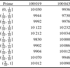
. The numerical evidence seems to support this. For a given prime
 $p\equiv 2\;(\text{mod}\;3)$
and every
 $c=1,\ldots ,p-1$
we compute the length,
 $l(c,p)$
, say, of the cycle which starts at
 $m=0$
. We then see for how many values of
 $c$
the scaled cycle length
 $p^{-1}l(c,p)$
falls into each of the intervals
 $((k-1)/10,k/10]$
for
 $k=1,\ldots ,10$
. If the permutations induced by the various polynomials
 $X^{3}+c$
were genuinely random, we would expect roughly the same number of scaled cycle lengths in each such interval. The data for the first two primes
 $p\equiv 2\;(\text{mod}\;3)$
beyond
 $10^{5}$
are presented in Table 1. The figures appear to support the random permutation model well.
Distribution of scaled cycle lengths.

However, the random permutation model would predict that one has four or more fixed points in a positive proportion of cases, while a polynomial
 $X^{3}+c$
can have at most three fixed points.
The main goal of the present paper is to describe a quite different theory for the iterates of quadratic polynomials in odd characteristic, in which it is clear why the anomalous cases above must be excluded. In contrast to the situation with
 $f(X)=X^{3}+1$
, when
 $f(X)=aX^{2}+bX+c$
, the equation
 $f(x)=s$
typically has either two solutions or none at all, the latter case holding for roughly half of the possible values of
 $s$
(those for which
 $b^{2}-4a(c-s)$
is a non-square). When
 $f(x)=s$
has two solutions
 $x=t_{1}$
and
 $x=t_{2}$
, the equations
 $f(x)=t_{1}$
and
 $f(x)=t_{2}$
will again typically have either two solutions or none. In this way, considering solutions of
 $f^{r}(x)=m$
, one sees that
 $\unicode[STIX]{x1D6E4}_{f}$
is potentially much more complicated than a series of cycles.
Our main result demonstrates this distinction clearly.
Theorem 1. Let
 $\mathbb{F}_{q}$
be a finite field of characteristic
 $p\not =2$
and let
 $f(X)=aX^{2}+c\in \mathbb{F}_{q}[X]$
, with
 $a\not =0$
. Suppose that
 $f^{i}(0)\not =f^{j}(0)$
for
 $0\leqslant i<j\leqslant r$
. Then
 $$\begin{eqnarray}\#f^{r}(\mathbb{F}_{q})=\unicode[STIX]{x1D707}_{r}q+O(2^{4^{r}}\sqrt{q})\end{eqnarray}$$
uniformly in
 $a$
and
 $c$
, where the constant
 $\unicode[STIX]{x1D707}_{r}$
is defined recursively by taking
 $\unicode[STIX]{x1D707}_{0}=1$
and
 $$\begin{eqnarray}\unicode[STIX]{x1D707}_{r+1}=\unicode[STIX]{x1D707}_{r}-{\textstyle \frac{1}{2}}\unicode[STIX]{x1D707}_{r}^{2}.\end{eqnarray}$$
Moreover, we have
 $\unicode[STIX]{x1D707}_{r}\sim 2/r$
as
 $r\rightarrow \infty$
.
At this point we should mention some closely related work. Shao [Reference Shao5, Theorem 1.6] handled the case
 $f(X)=X^{2}+1$
by a method which generalizes readily to other quadratics. The condition in his theorem is stronger than ours (that
 $f^{i}(0)\not =f^{j}(0)$
for
 $0\leqslant i<j\leqslant r$
) but an examination of the proof shows that he only needs something like our condition. His result does not include an explicit dependence on
 $r$
. Juul et al [Reference Juul, Kurlberg, Madhu and Tucker3] handled general rational functions rather than restricting to quadratic polynomials. Their emphasis is on the reductions of a given rational function
 $\unicode[STIX]{x1D719}(X)\in \mathbb{Q}(X)$
modulo different primes, but they showed under quite general conditions that the sum of all cycle lengths is
 $o(p)$
as
 $p\rightarrow \infty$
. (See Corollary 2 below.)
Before discussing the implications of the theorem, let us examine the condition that
 $f^{i}(0)\not =f^{j}(0)$
for
 $0\leqslant i<j\leqslant r$
. The critical points of a polynomial
 $f(X)$
are the roots
 $\unicode[STIX]{x1D709}$
of
 $f^{\prime }(X)$
, and
 $f$
is said to be “post-critically finite” if the iterates
 $f^{j}(\unicode[STIX]{x1D709})$
eventually enter a cycle for every critical point
 $\unicode[STIX]{x1D709}$
. In dynamics in general post-critically finite maps are a very important subclass. Of course, over a finite field every polynomial is post-critically finite. However, our condition can be viewed as saying that, in an approximate sense,
 $f$
fails to be post-critically finite. (When
 $f(X)=aX^{2}+c$
, the only critical point is
 $\unicode[STIX]{x1D709}=0$
.)
Certainly the condition that
 $f^{i}(0)\not =f^{j}(0)$
for
 $0\leqslant i<j\leqslant r$
fails for the polynomials
 $f(X)=X^{2}$
and
 $f(X)=X^{2}-2$
, with
 $i=0,j=1$
and
 $i=2,j=3$
, respectively. Suppose next that
 $f$
is the reduction of a polynomial
 $F(X)=AX^{2}+C\in \mathbb{Z}[X]$
, with
 $A,C>0$
; then the sequence
 $F^{0}(0),F^{1}(0),F^{2}(0),\ldots$
is strictly monotonic, with
 $F^{j}(0)\leqslant (A+C)^{2^{j}-1}$
. Thus, if
 $p\geqslant (A+C)^{2^{r}}$
, we cannot have
 $p\mid F^{j}(0)-F^{i}(0)$
, with
 $0\leqslant i<j\leqslant r$
. The condition of the theorem will therefore hold when
 $$\begin{eqnarray}r\leqslant \frac{\log \log p}{\log 2}-\frac{\log \log (A+C)}{\log 2}.\end{eqnarray}$$
In following this paper, the reader may wish to bear in mind the archetypal example
 $f(X)=X^{2}+1$
, for which
 $r\leqslant {\textstyle \frac{1}{2}}\log \log p$
suffices.
Our main theorem above has the following immediate consequences.
Corollary 1. Let
 $\mathbb{F}_{q}$
be a finite field of characteristic
 $p\not =2$
and let
 $f(X)=aX^{2}+c\in \mathbb{F}_{q}[X]$
, with
 $a\not =0$
. Then
 $f^{i}(0)=f^{j}(0)$
for some
 $i,j$
with
 $$\begin{eqnarray}i<j\ll \frac{q}{\log \log q}.\end{eqnarray}$$
Corollary 2. Let
 $\mathbb{F}_{p}$
be a finite field with
 $p>2$
prime and let
 $f(X)=aX^{2}+c\in \mathbb{F}_{p}[X]$
be the reduction of
 $AX^{2}+C\in \mathbb{Z}[X]$
, where
 $A,C>0$
. Then the sum of all the cycle lengths in
 $\unicode[STIX]{x1D6E4}_{f}$
will be
 $O_{A,C}(p(\log \log p)^{-1})$
. Similarly, the length of any pre-cyclic path in
 $\unicode[STIX]{x1D6E4}_{f}$
will be
 $O_{A,C}(p(\log \log p)^{-1})$
.
The first corollary gives an unconditional bound
 $o(q)$
for the first recurrence in the sequence
 $f^{0}(0),f^{1}(0),f^{2}(0),\ldots .$
The second corollary proves a similar result for arbitrary initial values for the reductions of fixed positive-definite quadratic polynomials
 $AX^{2}+C$
. Moreover, it highlights the difference in behaviour between such polynomials and the cubic case
 $f(X)=X^{3}+1$
, where the cycle lengths can sum to
 $q$
.
To prove Corollary 1, we choose
 $r=[(\log \log q)/(\log 4)]-1$
, so that
 $2^{4^{r}}\sqrt{q}\ll q/r$
. Then, according to Theorem 1, we have either
 $f^{i}(0)=f^{j}(0)$
for some
 $i<j\leqslant r$
or
 $\#f^{r}(\mathbb{F}_{q})\ll q/r$
. Writing the latter bound as
 $\#f^{r}(\mathbb{F}_{q})\leqslant Cq/r$
for an appropriate constant
 $C$
, we deduce in the latter case that if
 $k=[Cq/r]$
then the values
 $f^{r}(0),f^{r+1}(0),\ldots ,f^{r+k}(0)$
cannot be distinct, since they all lie in
 $f^{r}(\mathbb{F}_{q})$
and
 $k+1>Cq/r$
. In either case there must therefore be acceptable values
 $i<j\leqslant r+k$
. The claim then follows.
For Corollary 2, we observe as above that the condition of the theorem holds under the assumption (3). The choice
 $r=[(\log \log p)/(\log 4)]-1$
will satisfy (3) when
 $p\gg _{A,C}1$
and the theorem then yields
 $\#f^{r}(\mathbb{F}_{p})\ll p/r$
. All cycles lie inside
 $f^{r}(\mathbb{F}_{p})$
, giving the first assertion of the corollary. Moreover, if
 $f^{0}(m),\ldots ,f^{t}(m)$
is a pre-cyclic path, then
 $f^{r}(m),\ldots ,f^{t}(m)$
are distinct elements in
 $f^{r}(\mathbb{F}_{p})$
, so that
 $t-r\ll p/r$
. We then see that
 $t\ll r+p/r$
, from which the second assertion follows.
We should explain the restriction to polynomials
 $aX^{2}+c$
. For an arbitrary polynomial
 $f$
, if we define
 $g(X):=f(X+d)-d$
, then we will have
 $g^{j}(X)=f^{j}(X+d)-d$
. Thus,
 $\unicode[STIX]{x1D6E4}_{g}$
may be obtained from
 $\unicode[STIX]{x1D6E4}_{f}$
by relabelling each vertex
 $m$
as
 $m-d$
. Since the two graphs are isomorphic in this sense, it suffices to study
 $f(X+d)-d$
for a suitably chosen
 $d$
. In the case in which
 $f(X)=aX^{2}+bX+c$
(and
 $\mathbb{F}_{q}$
has odd characteristic), we can choose
 $d=-b/(2a)$
to produce a polynomial
 $g(X)$
of the shape
 $aX^{2}+c^{\prime }$
. Thus, we may translate our results into statements about general quadratic polynomials as follows.
Corollary 3. Let
 $\mathbb{F}_{q}$
be a finite field of characteristic
 $p\not =2$
and let
 $f(X)=aX^{2}+bX+c\in \mathbb{F}_{q}[X]$
, with
 $a\not =0$
. Suppose that
 $f^{i}(-b/(2a))\not =f^{j}(-b/(2a))$
for
 $0\leqslant i<j\leqslant r$
. Then
 $$\begin{eqnarray}\#f^{r}(\mathbb{F}_{q})=\unicode[STIX]{x1D707}_{r}q+O(2^{4^{r}}\sqrt{q})\end{eqnarray}$$
uniformly in
 $a,b$
and
 $c$
, with the same
 $\unicode[STIX]{x1D707}_{r}$
as before.
In particular,
 $f^{i}(-b/(2a))=f^{j}(-b/(2a))$
for some
 $i,j$
, with
 $$\begin{eqnarray}i<j\ll \frac{q}{\log \log q}.\end{eqnarray}$$
If
 $q$
is prime and
 $f$
is the reduction of a positive-definite quadratic polynomial
 $AX^{2}+BX+C\in \mathbb{Z}[X]$
, then the sum of all the cycle lengths in
 $\unicode[STIX]{x1D6E4}_{f}$
will be
 $O_{A,B,C}(q(\log \log q)^{-1})$
. Similarly, the length of any pre-cyclic path in
 $\unicode[STIX]{x1D6E4}_{f}$
will be
 $O_{A,B,C}(q(\log \log q)^{-1})$
.
In much the same way one can show that it would suffice to prove our theorem for polynomials
 $f(X)=X^{2}+d$
. One could then deduce the corresponding result for
 $aX^{2}+d/a$
by considering iterates of
 $g(X):=a^{-1}f(aX)$
.
Theorem 1 gives us an asymptotic formula
 $\#f^{r}(\mathbb{F}_{q})\sim \unicode[STIX]{x1D707}_{r}q$
. We proceed to give a probabilistic argument showing why one might expect this and how the recurrence relation (2) arises. When
 $r=0$
, we have
 $\#f^{0}(\mathbb{F}_{q})=q$
, so that
 $\unicode[STIX]{x1D707}_{0}=1$
. Suppose now that we have a relation
 $\#f^{r}(\mathbb{F}_{q})\sim \unicode[STIX]{x1D707}_{r}q$
. We will use an inductive argument to produce the corresponding result for
 $f^{r+1}$
.
To have
 $m\in f^{r+1}(\mathbb{F}_{q})$
, it is necessary and sufficient that
 $m\in f(\mathbb{F}_{q})$
and that
 $n\in f^{r}(\mathbb{F}_{q})$
for at least one solution
 $n$
of
 $f(x)=m$
. Since
 $\mathbb{F}_{q}$
contains
 $(q+1)/2$
squares, one has
 $m\in f(\mathbb{F}_{q})$
in exactly
 $(q+1)/2$
cases and, except for the value
 $m=f(0)$
, there will then be precisely two possible values of
 $n$
. Let these be
 $n_{1}$
and
 $n_{2}$
. If the probability of these lying in
 $f^{r}(\mathbb{F}_{q})$
were
 $\unicode[STIX]{x1D707}_{r}$
each, independently, one might expect that the probability of at least one being in
 $f^{r}(\mathbb{F}_{q})$
should be
 $2\unicode[STIX]{x1D707}_{r}-\unicode[STIX]{x1D707}_{r}^{2}$
, by the inclusion–exclusion principle. It would then follow that
 $m$
belongs to
 $f^{r+1}(\mathbb{F}_{q})$
with probability around
 ${\textstyle \frac{1}{2}}(2\unicode[STIX]{x1D707}_{r}-\unicode[STIX]{x1D707}_{r}^{2})$
. One would therefore produce an asymptotic expression
 $\#f^{r+1}(\mathbb{F}_{q})\sim \unicode[STIX]{x1D707}_{r+1}q$
, with
 $\unicode[STIX]{x1D707}_{r+1}$
as in (2).
We next explain why
 $\unicode[STIX]{x1D707}_{r}\sim 2r^{-1}$
, as claimed in Theorem 1. Writing
 $\unicode[STIX]{x1D708}_{r}=2/\unicode[STIX]{x1D707}_{r}$
, we see that
 $\unicode[STIX]{x1D708}_{0}=2$
and
 $$\begin{eqnarray}\unicode[STIX]{x1D708}_{r+1}=\unicode[STIX]{x1D708}_{r}+1+\frac{1}{\unicode[STIX]{x1D708}_{r}-1}.\end{eqnarray}$$
An easy induction then shows that
 $\unicode[STIX]{x1D708}_{r}\geqslant r+2$
for all
 $r\geqslant 0$
, whence
 $\unicode[STIX]{x1D708}_{r+1}\leqslant \unicode[STIX]{x1D708}_{r}+1+1/(r+1)$
. Another induction shows that
 $$\begin{eqnarray}\unicode[STIX]{x1D708}_{r}\leqslant r+2+\mathop{\sum }_{j=1}^{r}j^{-1},\quad (r\geqslant 1),\end{eqnarray}$$
so that
 $\unicode[STIX]{x1D708}_{r}\leqslant r+3+\log r$
for
 $r\geqslant 1$
. Together with the lower bound
 $\unicode[STIX]{x1D708}_{r}\geqslant r+2$
, this shows that
 $\unicode[STIX]{x1D708}_{r}\sim r$
and hence
 $\unicode[STIX]{x1D707}_{r}\sim 2/r$
.
2 A second moment calculation
Fundamental to our treatment of Theorem 1 will be moments of the functions
 $$\begin{eqnarray}\unicode[STIX]{x1D70C}_{r}(m)=\#\{x\in \mathbb{F}_{q}:f^{r}(x)=m\}.\end{eqnarray}$$
Our first task is to estimate the moments
 $$\begin{eqnarray}N(r;k):=\mathop{\sum }_{m\in \mathbb{F}_{q}}\unicode[STIX]{x1D70C}_{r}(m)^{k}\end{eqnarray}$$
for
 $r=0,1,2,\ldots$
and
 $k=1,2,\ldots .$
Trivially we have
 $\unicode[STIX]{x1D70C}_{0}(m)=1$
for all
 $m$
, so that
 $N(0;k)=q$
for every
 $k$
. Moreover, it is also clear that
 $N(r;1)=q$
for every
 $r$
.
Before moving to the general situation, it may be helpful to think first about the case
 $k=2$
, for which
 $$\begin{eqnarray}N(r;2)=\#\{(x,y)\in \mathbb{F}_{q}^{2}:f^{r}(x)=f^{r}(y)\}.\end{eqnarray}$$
The equation
 $f^{r}(X)-f^{r}(Y)=0$
defines a curve in
 $\mathbb{A}^{2}$
. An absolutely irreducible curve
 $C$
over
 $\mathbb{F}_{q}$
will have
 $q+O_{C}(\sqrt{q})$
points, by Weil’s “Riemann hypothesis”. However, our curve is far from being irreducible.
Indeed,
 $$\begin{eqnarray}f^{r}(X)-f^{r}(Y)=a(f^{r-1}(X)+f^{r-1}(Y))(f^{r-1}(X)-f^{r-1}(Y)),\end{eqnarray}$$
whence a trivial induction produces
 $$\begin{eqnarray}f^{r}(X)-f^{r}(Y)=a^{r}(X-Y)\mathop{\prod }_{j=0}^{r-1}(f^{j}(X)+f^{j}(Y)).\end{eqnarray}$$
Thus, we obtain
 $r+1$
factors. However, it is not immediately clear when polynomials of the form
 $f^{j}(X)+f^{j}(Y)$
are absolutely irreducible over
 $\mathbb{F}_{q}$
.
In general, suppose that
 $\unicode[STIX]{x1D719}(X,Y)$
is a polynomial of degree
 $D$
, over a field
 $K$
, and let
 $\unicode[STIX]{x1D6F7}(U,V,W)=W^{D}\unicode[STIX]{x1D719}(U/W,V/W)$
be the corresponding form. If
 $\unicode[STIX]{x1D6F7}$
factors as
 $\unicode[STIX]{x1D6F7}_{1}\unicode[STIX]{x1D6F7}_{2}$
over the algebraic completion
 $\overline{K}$
, then there will necessarily be a triple
 $(u,v,w)\not =(0,0,0)\in \overline{K}^{3}$
such that
 $\unicode[STIX]{x1D6F7}_{1}(u,v,w)=\unicode[STIX]{x1D6F7}_{2}(u,v,w)=0$
. For any such triple, we then have
 $\unicode[STIX]{x1D6FB}\unicode[STIX]{x1D6F7}=\unicode[STIX]{x1D6F7}_{1}\unicode[STIX]{x1D6FB}\unicode[STIX]{x1D6F7}_{2}+\unicode[STIX]{x1D6F7}_{2}\unicode[STIX]{x1D6FB}\unicode[STIX]{x1D6F7}_{1}=\mathbf{0}$
. This gives us a simple criterion for absolute irreducibility, which is sufficient, though not necessary: if
 $\unicode[STIX]{x1D6FB}\unicode[STIX]{x1D6F7}$
vanishes only at the origin in
 $\overline{K}^{3}$
, then
 $\unicode[STIX]{x1D6F7}$
must be absolutely irreducible.
We apply this criterion to
 $f^{j}(X)+f^{j}(Y)$
. Writing
 $D=2^{j}$
for convenience, and
 $$\begin{eqnarray}F^{j}(U,W)=W^{D}f^{j}(U/W),\end{eqnarray}$$
we have
 $$\begin{eqnarray}\displaystyle & & \displaystyle \unicode[STIX]{x1D6FB}(F^{j}(U,W)+F^{j}(V,W))\nonumber\\ \displaystyle & & \displaystyle ~~=\biggl(\!W^{D-1}(f^{j})^{\prime }(U/W),W^{D-1}(f^{j})^{\prime }(V/W),\frac{\unicode[STIX]{x2202}}{\unicode[STIX]{x2202}W}(F^{j}(U,W)+F^{j}(V,W))\!\biggr).\nonumber\end{eqnarray}$$
If
 $f(X)=aX^{2}+c$
, then
 $(f^{j})^{\prime }(X)=2af^{j-1}(X)(f^{j-1})^{\prime }(X)$
. It then follows by induction that
 $$\begin{eqnarray}W^{D-1}(f^{j})^{\prime }(U/W)=(2a)^{j}\mathop{\prod }_{s=0}^{j-1}F^{s}(U,W).\end{eqnarray}$$
In particular, if
 $\unicode[STIX]{x1D6FB}(F^{j}(u,w)+F^{j}(v,w))$
vanishes, then there are indices
 $s,t\leqslant j-1$
for which
 $F^{s}(u,w)=F^{t}(v,w)=0$
. Since
 $$\begin{eqnarray}F^{s}(u,0)=a^{2^{s}-1}u^{2^{s}}\quad \text{and}\quad F^{t}(v,0)=a^{2^{t}-1}v^{2^{t}},\end{eqnarray}$$
we see that
 $w=0$
would imply
 $u=v=w=0$
, which is excluded. We then see that we would have
 $f^{s}(x)=f^{t}(y)=0$
for some values
 $x,y\in \overline{K}$
such that
 $f^{j}(x)+f^{j}(y)=0$
. However,
 $f^{j}(x)=f^{j-s}(f^{s}(x))=f^{j-s}(0)$
and similarly for
 $f^{j}(y)$
. It follows that if
 $f^{j}(X)+f^{j}(Y)$
fails to be absolutely irreducible, then
 $f^{j-s}(0)+f^{j-t}(0)=0$
for some pair of non-negative integers
 $s,t\leqslant j-1$
. If
 $s=t$
, then, since
 $\mathbb{F}_{q}$
has odd characteristic, we have
 $f^{j-s}(0)=0=f^{0}(0)$
, with
 $1\leqslant j-s\leqslant j$
. Otherwise
 $f^{j-s+1}(0)=f^{j-t+1}(0)$
, with distinct positive integers
 $j-s+1,j-t+1\leqslant j+1$
. Since Theorem 1 assumes that the values
 $f^{0}(0),f^{1}(0),\ldots ,f^{r}(0)$
are distinct, we therefore conclude that the polynomial
 $f^{j}(X)+f^{j}(Y)$
is irreducible over the algebraic completion
 $\overline{\mathbb{F}_{q}}$
for every
 $j<r$
.
We are now ready to estimate
 $N(r;2)$
. In view of (4) and (5), we have
 $$\begin{eqnarray}N(r;2)\leqslant q+\mathop{\sum }_{j=0}^{r-1}\#\{(x,y)\in \mathbb{F}_{q}^{2}:f^{j}(x)+f^{j}(y)=0\},\end{eqnarray}$$
there being
 $q$
solutions to
 $x-y=0$
. To get a corresponding lower bound, we may use the inclusion–exclusion principle to show that
 $N(r;2)$
is at least
 $$\begin{eqnarray}q+\mathop{\sum }_{j=0}^{r-1}\#\{(x,y)\in \mathbb{F}_{q}^{2}:f^{j}(x)+f^{j}(y)=0\}-\mathop{\sum }_{0\leqslant j\leqslant r-1}A_{j}-\mathop{\sum }_{0\leqslant i<j\leqslant r-1}B_{ij},\end{eqnarray}$$
where
 $A_{j}$
is the number of common solutions to
 $$\begin{eqnarray}X-Y=0\quad \text{and}\quad f^{j}(X)+f^{j}(Y)=0\end{eqnarray}$$
and
 $B_{ij}$
is the number of common solutions to
 $$\begin{eqnarray}f^{i}(X)+f^{i}(Y)=0\quad \text{and}\quad f^{j}(X)+f^{j}(Y)=0.\end{eqnarray}$$
However, if
 $f^{j}(x)+f^{j}(y)=0$
, with
 $x=y$
, then
 $f^{j}(x)=0$
, which has at most
 $2^{j}$
solutions. Thus,
 $A_{j}\leqslant 2^{j}$
. Similarly, if
 $(x,y)$
were to lie on two distinct curves
 $f^{j}(X)+f^{j}(Y)=0$
and
 $f^{i}(X)+f^{i}(Y)=0$
, with
 $0\leqslant i<j\leqslant r-1$
, then
 $$\begin{eqnarray}f^{j}(y)=f^{j-i}(f^{i}(y))=f^{j-i}(-f^{i}(x))=f^{j}(x),\end{eqnarray}$$
since
 $f^{j-i}$
is an even polynomial. We would then have
 $2f^{j}(x)=0$
, so that
 $x$
, and similarly
 $y$
, would be a root of
 $f^{j}$
. There are therefore at most
 $2^{j}$
choices for
 $x$
and, since
 $y$
then satisfies
 $f^{i}(y)=-f^{i}(x)$
, there are at most
 $2^{i}$
choices of
 $y$
for each possible
 $x$
. Thus,
 $B_{ij}\leqslant 2^{j+i}$
. It follows that
 $$\begin{eqnarray}\mathop{\sum }_{0\leqslant j\leqslant r-1}A_{j}\leqslant 2^{r}\quad \text{and}\quad \mathop{\sum }_{0\leqslant i<j\leqslant r-1}B_{ij}\leqslant 2^{2r}.\end{eqnarray}$$
We therefore conclude that
 $$\begin{eqnarray}N(r;2)=q+\mathop{\sum }_{j=0}^{r-1}\#\{(x,y)\in \mathbb{F}_{q}^{2}:f^{j}(x)+f^{j}(y)=0\}+O(4^{r}).\end{eqnarray}$$
It remains to count points on the curves
 $f^{j}(X)+f^{j}(Y)=0$
. We have already shown that these are absolutely irreducible, and indeed non-singular, under the assumptions of Theorem 1. If we write
 $N_{r}$
for the number of projective points on the curve, and
 $D=2^{j}$
for its degree, then Weil’s “Riemann hypothesis” tells us that
 $$\begin{eqnarray}|N_{r}-(q+1)|\leqslant (D-1)(D-2)\sqrt{q}.\end{eqnarray}$$
There are at most
 $D$
points at infinity, so that
 $$\begin{eqnarray}|\#\{(x,y)\in \mathbb{F}_{q}^{2}:f^{j}(x)+f^{j}(y)=0\}-q|\leqslant D^{2}\sqrt{q}.\end{eqnarray}$$
Finally, summing for
 $0\leqslant j\leqslant r-1$
, we find that
 $$\begin{eqnarray}\mathop{\sum }_{j=0}^{r-1}\#\{(x,y)\in \mathbb{F}_{q}^{2}:f^{j}(x)+f^{j}(y)=0\}=rq+O(4^{r}\sqrt{q}).\end{eqnarray}$$
We may therefore summarize the conclusions of this section as follows.
Lemma 1. Under the assumptions of Theorem 1, we have
 $$\begin{eqnarray}N(r;2):=\mathop{\sum }_{m\in \mathbb{F}_{q}}\unicode[STIX]{x1D70C}_{r}(m)^{2}=(r+1)q+O(4^{r}\sqrt{q}).\end{eqnarray}$$
3 Higher moments—irreducible curves
We now develop the ideas of the previous section to estimate
 $N(r;k)$
for
 $k\geqslant 3$
. Here
 $N(r;k)$
is the number of solutions of
 $$\begin{eqnarray}f^{r}(x_{1})=\cdots =f^{r}(x_{k})\end{eqnarray}$$
in
 $\mathbb{F}_{q}$
. These equations define a curve, but, as in the previous section, it is far from being an irreducible curve. Our task in this section is to identify the absolutely irreducible components and to show that they are all defined over
 $F_{q}$
.
In view of (5), for any solution of (7) and any pair of distinct indices
 $1\leqslant i,j\leqslant k$
, there is a corresponding
 $$\begin{eqnarray}d=d(i,j)=d(j,i)\in \{-1,0,1,\ldots ,r-1\}\end{eqnarray}$$
such that
 $\unicode[STIX]{x1D719}(x_{i},x_{j};d)=0$
, where
 $$\begin{eqnarray}\unicode[STIX]{x1D719}(X,Y;d)=\left\{\begin{array}{@{}ll@{}}f^{d}(X)+f^{d}(Y), & d\geqslant 0,\\ X-Y, & d=-1.\end{array}\right.\end{eqnarray}$$
If there is more than one choice for
 $d(i,j)$
, we choose the smallest.
We now make the following definition.
Definition 1. A “
 $(D,k)$
-graph” is a weighted graph on
 $k$
vertices for which any edge
 $ij$
has integral weight in the range
 $[-1,D]$
. If some edge has weight equal to
 $D$
, we say that we have a “strict
 $(D,k)$
-graph”. If there is an edge between every pair of vertices, we say that we have a “complete
 $(D,k)$
-graph”.
Thus, each solution of (7) produces a complete
 $(D,k)$
-weighted graph. We now introduce the following further definition.
Definition 2. Let
 $G$
be a complete
 $(D,k)$
-graph. Then we say that
 $G$
is “proper” if, whenever
 $a,b,c$
are distinct vertices, with
 $d(a,b)\leqslant d(a,c)$
 ${\leqslant}d(b,c)$
, then either
 $d(a,b)=d(a,c)=d(b,c)=-1$
or
 $d(a,b)<$
 $d(a,c)=d(b,c)$
.
We then have the following lemma.
Lemma 2. The graph associated to a solution of (7) is proper.
To prove the claim, observe firstly that if
 $d(a,b)=d(a,c)=-1$
, then
 $x_{a}=x_{b}$
and
 $x_{a}=x_{c}$
, whence
 $x_{a}=x_{c}$
, so that
 $d(b,c)=-1$
. Next we show that one cannot have
 $d(a,b)=d(a,c)\geqslant 0$
. Writing
 $d=d(a,b)=d(a,c)$
, this would imply
 $f^{d}(x_{a})=-f^{d}(x_{b})$
and
 $f^{d}(x_{a})=-f^{d}(x_{c})$
, whence
 $$\begin{eqnarray}f^{d}(x_{b})-f^{d}(x_{c})=0.\end{eqnarray}$$
The factorization (5) would then show that
 $\unicode[STIX]{x1D719}(x_{b},x_{c};e)=0$
for some
 $e<d\leqslant d(b,c)$
. This however is impossible, since
 $d(b,c)$
was chosen minimally.
To complete the proof of the claim, we show that if
 $$\begin{eqnarray}d(a,b)<d(a,c)\leqslant d(b,c),\end{eqnarray}$$
then
 $d(a,c)=d(b,c)$
. In view of (5), the relation
 $\unicode[STIX]{x1D719}(x_{a},x_{b};d(a,b))=0$
would imply
 $f^{d(a,c)}(X_{a})-f^{d(a,c)}(X_{b})=0$
. Since
 $$\begin{eqnarray}\unicode[STIX]{x1D719}(X_{a},X_{c};d(a,c))=f^{d(a,c)}(X_{a})+f^{d(a,c)}(X_{c})=0,\end{eqnarray}$$
this would show that
 $f^{d(a,c)}(X_{b})+f^{d(a,c)}(X_{c})=0$
and the minimal choice of
 $d(b,c)$
then produces
 $d(b,c)\leqslant d(a,c)$
, giving the required conclusion. This now establishes the lemma in full.
Thus, each solution of (7) is associated to a unique proper weighted graph such that
 $$\begin{eqnarray}\unicode[STIX]{x1D719}(x_{i},x_{j};d(i,j))=0\quad (1\leqslant i\not =j\leqslant k).\end{eqnarray}$$
However, there is considerable redundancy in the equations (8). To investigate this, we begin with the following result.
Lemma 3. Let
 $G$
be a proper strict
 $(D,k)$
-graph, with
 $D\geqslant 0$
. Then there is a unique partition
 $\{1,\ldots ,k\}=A\cup B$
into non-empty sets
 $A$
and
 $B$
such that
 $d(a,b)=D$
when
 $a\in A$
and
 $b\in B$
, while
 $d(i,j)<D$
whenever
 $i,j\in A$
or
 $i,j\in B$
.
Firstly it is easy to see that such a partition must be unique. For, if
 $A^{\prime }\cup B^{\prime }$
were a different partition, then, after relabelling if necessary, we could find indices
 $i,j\in A$
, with
 $i\in A^{\prime }$
and
 $j\in B^{\prime }$
. We would then have both
 $d(i,j)<D$
(because
 $i,j\in A$
) and
 $d(i,j)=D$
(because
 $i\in A^{\prime }$
and
 $j\in B^{\prime }$
). This contradiction shows that such partitions are unique.
In order to show the existence of a suitable partition, we fix a pair
 $i_{0},j_{0}$
, with
 $d(i_{0},j_{0})=D$
, and let
 $$\begin{eqnarray}A=\cup \{i:d(i,j_{0})=D\},\qquad B=\{j:d(j,i_{0})=D\}.\end{eqnarray}$$
Then
 $i_{0}\in A$
and
 $j_{0}\in B$
, so that neither set is empty. If
 $a$
, say, were in
 $A\cap B$
, then
 $$\begin{eqnarray}d(a,j_{0})=d(a,i_{0})=d(i_{0},j_{0})=D\geqslant 0,\end{eqnarray}$$
contradicting Definition 2. For any
 $a\in \{1,\ldots ,k\}$
, Definition 2 shows that we must have either
 $d(a,i_{0})=D$
or
 $d(a,j_{0})=D$
, so that
 $A\cup B$
is a partition of
 $\{1,\ldots ,k\}$
.
If
 $a_{1},a_{2}\in A$
had
 $d(a_{1},a_{2})=D$
, then the triple
 $a_{1},a_{2},j_{0}$
would contradict Definition 2. Thus,
 $d(a_{1},a_{2})<D$
and similarly
 $d(b_{1},b_{2})<D$
when
 $b_{1},b_{2}\in B$
. Finally, if
 $a_{1}\in A$
, then
 $d(a_{1},j_{0})=D$
if
 $a_{1}=i_{0}$
. Otherwise Definition 2 applied to the triple
 $a_{1},i_{0},j_{0}$
shows one that
 $d(a_{1},j_{0})=D$
, since
 $d(a_{1},i_{0})<D$
. Thus,
 $d(a,j_{0})=D$
for all
 $a\in A$
. Now, if
 $b\in B$
, with
 $b\not =j_{0}$
, Definition 2 applied to the triple
 $a,b,j_{0}$
shows that
 $d(a,b)=D$
, since
 $d(b,j_{0})<D$
. Hence,
 $d(a,b)=D$
whenever
 $a\in A$
and
 $b\in B$
. This completes the proof of the lemma.
We now show how a complete
 $(D,k)$
-graph can be generated by a smaller graph.
Definition 3. Let
 $G$
be a complete
 $(D,k)$
-graph and suppose that
 $G_{0}$
is a subgraph of
 $G$
with the same set of vertices but fewer edges. We then say that
 $G_{0}$
“generates”
 $G$
if
 $G=G_{n}$
for some
 $n$
, where
 $G_{h+1}$
is obtained from
 $G_{h}$
by the following procedure.
Take three distinct vertices
 $a,b,c$
for which the edges
 $ab$
and
 $bc$
belong to
 $G_{h}$
but
 $ac$
does not, and for which either
 $d(a,b)=d(b,c)=-1$
or
 $d(a,b)<d(b,c)$
. Then
 $G_{h+1}$
is obtained from
 $G_{h}$
by adding the edge
 $ac$
with weight
 $d(a,c)=d(b,c)$
.
For our purposes it is not necessary to know whether, using a different sequence of edge additions,
 $G_{0}$
might generate two different complete
 $(D,k)$
-graphs. All we need to know is whether there exists some sequence of edge additions resulting in
 $G$
.
To motivate the definition, we consider the ideal
 $I_{h}\subseteq \mathbb{F}_{q}[X_{1},\ldots ,X_{k}]$
generated by those polynomials
 $\unicode[STIX]{x1D719}(X_{i},X_{j};d(i,j))$
for which the edge
 $ij$
is in
 $G_{h}$
. Then trivially we have
 $I_{h}\subseteq I_{h+1}$
, since
 $I_{h+1}$
is formed from
 $I_{h}$
by the addition of one further generator
 $\unicode[STIX]{x1D719}(X_{a},X_{c},d(a,c))$
. If
 $d(a,b)=d(b,c)=-1$
in the procedure in Definition 3, we have
 $$\begin{eqnarray}\unicode[STIX]{x1D719}(X_{a},X_{b},d(a,b))=X_{a}-X_{b}\end{eqnarray}$$
and
 $$\begin{eqnarray}\unicode[STIX]{x1D719}(X_{b},X_{c},d(b,c))=X_{b}-X_{c}.\end{eqnarray}$$
Hence, if
 $d(a,c)=-1$
, then
 $$\begin{eqnarray}\unicode[STIX]{x1D719}(X_{a},X_{c},d(a,c))=X_{a}-X_{c}=\unicode[STIX]{x1D719}(X_{a},X_{b},d(a,b))+\unicode[STIX]{x1D719}(X_{b},X_{c},d(b,c)),\end{eqnarray}$$
so that
 $I_{h+1}=I_{h}$
. Alternatively, if
 $d(a,c)=d(b,c)>d(a,b)$
in the procedure in Definition 3, we have
 $$\begin{eqnarray}\displaystyle \unicode[STIX]{x1D719}(X_{a},X_{c},d(a,c)) & = & \displaystyle \unicode[STIX]{x1D719}(X_{a},X_{c},d(b,c))\nonumber\\ \displaystyle & = & \displaystyle f^{d(b,c)}(X_{a})+f^{d(b,c)}(X_{c})\nonumber\\ \displaystyle & = & \displaystyle (f^{d(b,c)}(X_{a})-f^{d(b,c)}(X_{b}))+\unicode[STIX]{x1D719}(X_{b},X_{c}:d(b,c)).\nonumber\end{eqnarray}$$
Here we have
 $\unicode[STIX]{x1D719}(X_{a},X_{b};d(a,b))\mid f^{d(b,c)}(X_{a})-f^{d(b,c)}(X_{b})$
by (5), since
 $d(a,b)<d(b,c)$
. Hence,
 $\unicode[STIX]{x1D719}(X_{a},X_{c},d(a,c))$
belongs to the ideal generated by
 $\unicode[STIX]{x1D719}(X_{a},X_{b},d(a,b))$
and
 $\unicode[STIX]{x1D719}(X_{b},X_{c},d(b,c))$
. We therefore see again that
 $I_{h+1}=I_{h}$
. It follows that if
 $G$
is the proper complete
 $(D,k)$
-graph associated to a system of equation (8), and
 $G$
is generated by
 $G_{0}$
, then the system (8) has the same solutions as the smaller system
 $$\begin{eqnarray}\unicode[STIX]{x1D719}(x_{i},x_{j};d(i,j))=0\quad (ij\text{ is an edge of }G_{0}).\end{eqnarray}$$
We now introduce the small graphs we shall use.
Definition 4. A
 $(D,k)$
-graph is said to be a “chain” if there is an ordering
 $i_{1},i_{2},\ldots$
of the vertices such that the edges are precisely the
 $k-1$
pairs
 $$\begin{eqnarray}(i_{1},i_{2}),(i_{2},i_{3}),\ldots ,(i_{k-1},i_{k})\end{eqnarray}$$
and, for any
 $s<t\leqslant k-1$
, the maximum of
 $$\begin{eqnarray}d(i_{s},i_{s+1}),\quad d(i_{s+1},i_{s+2}),\ldots ,d(i_{t},i_{t+1})\end{eqnarray}$$
is either
 $-1$
or is attained at only one point.
We then have the following result.
Lemma 4. For any proper
 $(D,k)$
-graph
 $G$
, there is a chain
 $(D,k)$
-graph
 $G_{0}$
which generates
 $G$
.
We prove this by induction on
 $D$
. If
 $D=-1$
, we may take
 $G_{0}$
to consist of the edges
 $(1,2),\ldots ,(k-1,k)$
, with weights
 $-1$
, which clearly generates
 $G$
. Now assume that the result is true for complete
 $(d,k)$
graphs, with
 $d\leqslant D-1$
. If
 $G$
is not a strict
 $(D,k)$
-graph, the conclusion is immediate from the induction hypothesis.
Thus, we assume that
 $G$
is a strict complete
 $(D,k)$
graph, with
 $D\geqslant 0$
, so that Lemma 3 applies. Let
 $G_{A}$
be the restriction of
 $G$
to the vertices in
 $A$
, so that
 $G_{A}$
is a complete
 $(D-1,m)$
-graph, where
 $m=\#A$
. The induction hypothesis then shows that there is a chain graph
 $G_{1}$
, say, which generates
 $G_{A}$
, in which one re-orders the vertices in
 $A$
as
 $i_{1},\ldots ,i_{m}$
so as to satisfy the chain property in Definition 4. Similarly, if
 $G_{B}$
is the restriction of
 $G$
to the vertices in
 $B$
, we can obtain a subgraph
 $G_{2}$
of
 $G_{B}$
which is a chain and which generates
 $G_{B}$
. If
 $n=\#B$
, there will again be an appropriate ordering
 $j_{1},\ldots ,j_{n}$
of the indices in
 $B$
.
We then take
 $G_{0}$
to be the graph with vertices
 $1,\ldots ,k$
whose edges are the edges of
 $G_{A}$
, the edges of
 $G_{B}$
and the additional edge
 $i_{m},j_{1}$
. Moreover, we permute the vertices into the order
 $i_{1},\ldots ,i_{m},j_{1},\ldots ,j_{n}$
. We claim firstly that this ordering makes
 $G_{0}$
a chain and secondly that
 $G_{0}$
generates
 $G$
.
To verify that
 $G_{0}$
is a chain, we consider a sequence of consecutive pairs of the vertices from the sequence
 $i_{1},\ldots ,i_{m},j_{1},\ldots ,j_{n}$
. If the sequence is entirely contained in the first
 $m$
terms, the required chain property follows from that for
 $G_{1}$
, and similarly if all the elements are taken from the last
 $n$
terms. However, if one of the pairs is the edge
 $i_{m},j_{1}$
it suffices to note that this edge has weight
 $D$
while all other edges have weight at most
 $D-1$
.
To check that
 $G_{0}$
generates
 $G$
, we note that
 $G_{1}$
generates
 $G_{A}$
and
 $G_{2}$
generates
 $G_{B}$
. Thus,
 $G_{0}$
certainly generates the graph
 $G^{\ast }$
containing the edges of
 $G_{A}$
, the edges of
 $G_{B}$
and the edge
 $i_{m},j_{1}$
. Hence, it suffices to show that
 $G^{\ast }$
generates
 $G$
. Let
 $ij$
be an edge of
 $G$
which is not already an edge in
 $G^{\ast }$
. Then, according to Lemma 3, we may assume that
 $i\in A$
and
 $j\in B$
and that
 $d(i,j)=D$
. Applying the procedure in Definition 3 to the triple
 $i,i_{m},j_{1}$
, we see that the edge
 $i,i_{m}$
is in
 $G^{\ast }$
, since
 $i,i_{m}\in A$
, and the edge
 $i_{m},j_{1}$
is also in
 $G^{\ast }$
, by definition. Moreover,
 $d(i,i_{m})<D=d(i_{m},j_{1})$
. Thus, the edge
 $i,j_{1}$
can be generated from
 $G^{\ast }$
, with weight
 $d(i,j_{1})=d(i_{m},j_{1})=D$
. We may then apply the procedure in Definition 3 to the triple
 $j,j_{1},i$
. This time the edge
 $j,j_{1}$
is in
 $G^{\ast }$
, since
 $j,j_{1}\in B$
, and the edge
 $j_{1},i$
can be generated from
 $G^{\ast }$
, as we have just shown. Moreover, we have
 $d(j,j_{1})<D=d(j_{1},i)$
, so that the edge
 $ji$
can also be generated from
 $G^{\ast }$
, and is given weight
 $D$
, as required. This completes the proof of the lemma.
As an immediate consequence of Lemma 4, we have the following.
Lemma 5. After a suitable relabelling of the variables, any solution to the equations (7) satisfies some system of equations of the type
 $$\begin{eqnarray}\unicode[STIX]{x1D719}(X_{i},X_{i+1};d_{i})=0\quad (1\leqslant i\leqslant k-1),\end{eqnarray}$$
with
 $-1\leqslant d_{i}\leqslant k-1$
. Moreover, if
 $1\leqslant i<j\leqslant k-1$
, then the maximum of
 $d_{i},\ldots ,d_{j}$
is either
 $-1$
or occurs at only one point.
We call a system of equations of the above type a “chain system”. The system defines a variety in
 $\mathbb{A}^{k}$
. We set
 $\unicode[STIX]{x1D6F7}(X,Y,Z;-1)=X-Y$
and
 $$\begin{eqnarray}\unicode[STIX]{x1D6F7}(X,Y,Z;d)=Z^{2^{d}}\unicode[STIX]{x1D719}(X/X,Y/Z;d)\quad (d\geqslant 0),\end{eqnarray}$$
so that the corresponding projective variety is given by
 $$\begin{eqnarray}{\mathcal{C}}:\unicode[STIX]{x1D6F7}(X_{i},X_{i+1},X_{0};d_{i})=0\quad (1\leqslant i\leqslant k-1).\end{eqnarray}$$
The importance of the chain property is demonstrated by the following result.
Lemma 6. Suppose that
 $f^{i}(0)\not =f^{j}(0)$
for
 $0\leqslant i<j\leqslant r$
. Then, for a chain system, the variety
 ${\mathcal{C}}$
is a non-singular complete intersection. Hence,
 ${\mathcal{C}}$
is an absolutely irreducible curve over
 $\mathbb{F}_{q}$
, with degree at most
 $2^{(k-1)(r-1)}$
.
To prove that
 ${\mathcal{C}}$
is a non-singular complete intersection, we need to show that the vectors
 $\unicode[STIX]{x1D6FB}\unicode[STIX]{x1D6F7}(x_{i},x_{i+1},x_{0};d_{i})$
are linearly independent at any point of
 ${\mathcal{C}}$
. Suppose to the contrary that
 $$\begin{eqnarray}\mathop{\sum }_{i=1}^{k-1}c_{i}\unicode[STIX]{x1D6FB}\unicode[STIX]{x1D6F7}(x_{i},x_{i+1},x_{0};d_{i})=\mathbf{0}.\end{eqnarray}$$
If the
 $c_{i}$
are not all zero, we take
 $s$
to be the smallest index with
 $c_{s}\not =0$
, and
 $t$
to be the largest index with
 $c_{t}\not =0$
, so that
 $$\begin{eqnarray}\mathop{\sum }_{i=s}^{t}c_{i}\unicode[STIX]{x1D6FB}\unicode[STIX]{x1D6F7}(x_{i},x_{i+1},x_{0};d_{i})=\mathbf{0}.\end{eqnarray}$$
The entries of this vector are labelled by the variables
 $X_{0},\ldots ,X_{k}$
, and one sees that the entry corresponding to
 $X_{s}$
is just
 $c_{s}(\unicode[STIX]{x2202}/\unicode[STIX]{x2202}x_{s})\unicode[STIX]{x1D6F7}(x_{s},x_{s+1},x_{0};d_{s})$
. We therefore conclude that
 $(\unicode[STIX]{x2202}/\unicode[STIX]{x2202}x_{s})\unicode[STIX]{x1D6F7}(x_{s},x_{s+1},x_{0};d_{s})=0$
and similarly that
 $(\unicode[STIX]{x2202}/\unicode[STIX]{x2202}x_{t+1})\unicode[STIX]{x1D6F7}(x_{t},x_{t+1},x_{0};d_{t})=0$
. In particular, we must have
 $d_{s},d_{t}\geqslant 1$
. However,
 $$\begin{eqnarray}\frac{\unicode[STIX]{x2202}}{\unicode[STIX]{x2202}x}\unicode[STIX]{x1D6F7}(x,y,z;d)=(2a)^{d}\mathop{\prod }_{i=0}^{d-1}F^{i}(x,z)\quad (d\geqslant 0)\end{eqnarray}$$
in the notation (6). We therefore see that
 $F^{i}(x_{s},x_{0})=0$
for some index
 $i$
in the range
 $0\leqslant i\leqslant d_{s}-1$
, and similarly
 $F^{j}(x_{t+1},x_{0})=0$
for some
 $j$
with
 $0\leqslant j\leqslant d_{t}-1$
.
We next show that
 $x_{0}$
cannot vanish. If, on the contrary, we had
 $x_{0}=0$
, then the relation
 $F^{i}(x_{s},x_{0})=0$
would yield
 $x_{s}=0$
. In general, if we have
 $x_{i}=x_{0}=0$
, then the relation
 $\unicode[STIX]{x1D6F7}(x_{i},x_{i+1},x_{0};d_{i})=0$
implies
 $x_{i+1}=0$
, while
 $\unicode[STIX]{x1D6F7}(x_{i-1},x_{i},x_{0};d_{i-1})=0$
implies
 $x_{i-1}=0$
. Thus, using both forwards and backwards induction, we would have
 $x_{i}=0$
for all
 $i$
, which is impossible.
We may therefore assume that
 $x_{0}=1$
, taking us back to the affine situation. Thus, we have
 $f^{i}(x_{s})=0$
and
 $f^{j}(x_{t+1})=0$
, with
 $0\leqslant i<d_{s}$
and
 $0\leqslant j<d_{t}$
. Since
 $d_{s}\geqslant 1$
, the chain property shows that the maximum of
 $d_{s},d_{s+1},\ldots ,d_{t}$
occurs at only one point,
 $d_{u}=D$
, say. Since
 $i<d_{s}\leqslant D$
, we have
 $f^{D}(x_{s})=f^{D-i}(f^{i}(x_{s}))=f^{D-i}(0)$
. Similarly, we have
 $f^{D}(x_{t+1})=f^{D-j}(0)$
. If
 $s\leqslant h<u$
, then
 $d_{h}<D$
, whence
 $\unicode[STIX]{x1D719}(X,Y;d_{h})\mid f^{D}(X)-f^{D}(Y)$
. Thus,
 $f^{D}(x_{h})=f^{D}(x_{h+1})$
for
 $s\leqslant h<u$
. It follows that
 $f^{D}(x_{u})=f^{D}(x_{s})=f^{D-i}(0)$
. Similarly, when
 $u<h\leqslant t$
, we have
 $f^{D}(x_{h})=f^{D}(x_{h+1})$
, whence
 $f^{D}(x_{u+1})=f^{D}(x_{t+1})=f^{D-j}(0)$
. However,
 $\unicode[STIX]{x1D719}(x_{u},x_{u+1};D)=0$
, with
 $D\geqslant 1$
, whence
 $f^{D}(x_{u})+f^{D}(x_{u+1})=0$
. As in the previous section, we therefore conclude that
 $f^{D-i}(0)+f^{D-j}(0)=0$
for some pair of non-negative integers
 $i,j<D$
. This leads either to
 $f^{D-i}(0)=0$
(if
 $i=j$
) or
 $f^{r}(0)=f^{r+i-j}(0)$
(if
 $i<j$
, say). In either case we contradict the assumption of Theorem 1, since
 $D\leqslant r$
. This completes the proof that
 ${\mathcal{C}}$
is a non-singular complete intersection.
The remainder of the lemma is now straightforward. In general a non-singular complete intersection is necessarily absolutely irreducible, with degree equal to the product of the degrees of the defining forms; see Browning and Heath-Brown [Reference Browning and Heath-Brown1, Lemma 3.2] for details. In our case
 $\unicode[STIX]{x1D6F7}(X_{i},X_{i+1},X_{0};d_{i})$
has degree at most
 $2^{r-1}$
, since
 $d_{i}\leqslant r-1$
, and the result follows.
4 Higher moments—counting points and counting curves
In this section we will firstly estimate the number of points on each curve
 ${\mathcal{C}}$
and then compute the number of such curves that the variety given by (7) produces. Putting these results together will give us an asymptotic formula for
 $N(r;k)$
.
Since
 ${\mathcal{C}}$
is an absolutely irreducible curve defined over
 $\mathbb{F}_{q}$
, Weil’s “Riemann hypothesis” yields
 $$\begin{eqnarray}|\#{\mathcal{C}}(\mathbb{F}_{q})-(q+1)|\leqslant 2g\sqrt{q},\end{eqnarray}$$
where
 $g$
is the genus of
 ${\mathcal{C}}$
. In general, if
 ${\mathcal{C}}$
is an irreducible non-degenerate curve of degree
 $d$
in
 $\mathbb{P}^{k}$
(with
 $k\geqslant 2$
), then, according to the Castelnuovo genus bound [Reference Castelnuovo2], one has
 $$\begin{eqnarray}g\leqslant (k-1)m(m-1)/2+m\unicode[STIX]{x1D700},\end{eqnarray}$$
where
 $d-1=m(k-1)+\unicode[STIX]{x1D700}$
, with
 $0\leqslant \unicode[STIX]{x1D700}<k-1$
. This implies in particular
 $g\leqslant (d-1)(d-2)/2$
irrespective of the degree of the ambient space in which
 ${\mathcal{C}}$
lies. We therefore deduce that
 $$\begin{eqnarray}|\#{\mathcal{C}}(\mathbb{F}_{q})-(q+1)|\leqslant 4^{kr}\sqrt{q},\end{eqnarray}$$
since
 ${\mathcal{C}}$
has degree at most
 $2^{kr}$
.
By inclusion–exclusion, and allowing for points at infinity, we see that
 $$\begin{eqnarray}\mathop{\sum }_{{\mathcal{C}}}(\#{\mathcal{C}}-2^{kr})(\mathbb{F}_{q})-\frac{1}{2}\mathop{\sum }_{{\mathcal{C}}_{1}\not ={\mathcal{C}}_{2}}\#({\mathcal{C}}_{1}\cap {\mathcal{C}}_{2})(\mathbb{F}_{q})\leqslant N(r;k)\leqslant \mathop{\sum }_{{\mathcal{C}}}\#{\mathcal{C}}(\mathbb{F}_{q}).\end{eqnarray}$$
For distinct curves of degree at most
 $2^{kr}$
, we have
 $$\begin{eqnarray}\#({\mathcal{C}}_{1}\cap {\mathcal{C}}_{2})(\mathbb{F}_{q})\leqslant 4^{kr},\end{eqnarray}$$
by Bézout’s theorem. Hence, if there are
 ${\mathcal{N}}(r;k)$
different curves
 ${\mathcal{C}}$
, we see that
 $$\begin{eqnarray}\biggl|N(r;k)-\mathop{\sum }_{{\mathcal{C}}}\#{\mathcal{C}}(\mathbb{F}_{q})\biggr|\leqslant {\mathcal{N}}(r;k)^{2}4^{kr}.\end{eqnarray}$$
We can get a crude bound for
 ${\mathcal{N}}(r;k)$
by observing that there are
 $k!$
possible permutations describing a chain system and, for each of the
 $k-1$
edges, one has
 $-1\leqslant d(\unicode[STIX]{x1D70E}(i),\unicode[STIX]{x1D70E}(i+1))\leqslant r-1$
. Thus, if
 $r\geqslant 1$
, we have
 $$\begin{eqnarray}{\mathcal{N}}(r;k)\leqslant k!(r+1)^{k-1}\leqslant k!(2r)^{k-1}\leqslant (rk)^{k}\leqslant (2^{r}k)^{k}.\end{eqnarray}$$
Applying (10), we then deduce the following result.
Lemma 7. If there are
 ${\mathcal{N}}(r;k)$
different curves
 ${\mathcal{C}}$
, then
 $$\begin{eqnarray}N(r;k)={\mathcal{N}}(r;k)(q+1)+O(2^{4kr}k^{2k}\sqrt{q}).\end{eqnarray}$$
Our task now is to investigate the number
 ${\mathcal{N}}(r;k)$
. We have seen that each curve
 ${\mathcal{C}}$
arises from a proper
 $(r-1,k)$
-graph. We proceed to show that different graphs
 $G,G^{\prime }$
cannot produce the same curve
 ${\mathcal{C}}$
. The graphs
 $G$
and
 $G^{\prime }$
must differ on at least one edge. Thus, for example, one would have both
 $\unicode[STIX]{x1D719}(X_{i},X_{j};d)=0$
and
 $\unicode[STIX]{x1D719}(X_{i},X_{j};d^{\prime })=0$
on
 ${\mathcal{C}}$
. If
 $d>d^{\prime }$
, say, then
 $f^{d}(X_{i})+f^{d}(X_{j})=0$
and
 $f^{d}(X_{i})-f^{d}(X_{j})=0$
, whence
 $f^{d}(X_{i})=0$
for all points on the curve. It then follows that
 $f^{r}(X_{i})=f^{r-d}(0)$
. However,
 ${\mathcal{C}}$
is an irreducible component of the curve (7), whence
 $f^{r}(X_{h})=f^{r}(X_{i})=f^{r-d}(0)$
for every index
 $h$
. This gives us a contradiction since it would imply that
 ${\mathcal{C}}$
has dimension zero.
We therefore need to count proper
 $(r-1,k)$
-graphs. For a proper strict
 $(D,k)$
-graph, Lemma 3 produces a unique partition
 $A\cup B$
, where the corresponding graphs
 $G_{A}$
and
 $G_{B}$
will be proper
 $(D-1,k)$
-graphs. There are
 ${\mathcal{N}}(r;k)-{\mathcal{N}}(r-1;k)$
proper strict
 $(r-1,k)$
-graphs. Moreover, the number of partitions
 $\{1,\ldots ,k\}=A\cup B$
with
 $a=\#A<\#B=b$
is
 $$\begin{eqnarray}\left(\begin{array}{@{}c@{}}k\\ a\end{array}\right),\end{eqnarray}$$
while, for even
 $k$
, the number with
 $a=b=k/2$
is
 $$\begin{eqnarray}\frac{1}{2}\left(\begin{array}{@{}c@{}}k\\ k/2\end{array}\right).\end{eqnarray}$$
We then see that
 $$\begin{eqnarray}{\mathcal{N}}(r;k)-{\mathcal{N}}(r-1;k)=\frac{1}{2}\mathop{\sum }_{a=1}^{k-1}\left(\begin{array}{@{}c@{}}k\\ a\end{array}\right){\mathcal{N}}(r-1;a){\mathcal{N}}(r-1;k-a)\end{eqnarray}$$
for
 $r\geqslant 1$
and
 $k\geqslant 2$
. Indeed, since
 ${\mathcal{N}}(r;1)=1$
for every
 $r$
, we see that this holds for
 $k=1$
too. If we now define
 ${\mathcal{N}}(r;0)=1$
for all
 $r\geqslant 0$
, the above formula simplifies to give
 $$\begin{eqnarray}{\mathcal{N}}(r;k)=\frac{1}{2}\mathop{\sum }_{a=0}^{k}\left(\begin{array}{@{}c@{}}k\\ a\end{array}\right){\mathcal{N}}(r-1;a){\mathcal{N}}(r-1;k-a)\quad (r,k\geqslant 1).\end{eqnarray}$$
We therefore define power series
 $$\begin{eqnarray}E(X;r):=\mathop{\sum }_{k=0}^{\infty }\frac{{\mathcal{N}}(r;k)}{k!}X^{k}\end{eqnarray}$$
for each
 $r\geqslant 1$
. Since (11) yields
 ${\mathcal{N}}(r;k)/k!\leqslant (r+1)^{k}$
, we see that this converges absolutely for
 $|X|<(r+1)^{-1}$
. Now, after checking that we have the correct coefficient for
 $X^{0}$
, we arrive at
 $$\begin{eqnarray}E(X;r)=\frac{1+E(X;r-1)^{2}}{2}\quad (r\geqslant 1).\end{eqnarray}$$
Since
 ${\mathcal{N}}(0;k)=1$
for all
 $k$
, we have
 $E(X;0)=\exp (X)$
, so that the coefficients
 ${\mathcal{N}}(r;k)$
can easily be calculated in general. Moreover, it is clear by induction that
 $$\begin{eqnarray}E(X;r)=\mathop{\sum }_{m=0}^{2^{r}}\unicode[STIX]{x1D708}(r;m)\text{e}^{mX},\end{eqnarray}$$
with non-negative real coefficients
 $\unicode[STIX]{x1D708}(r;m)$
summing to 1. We then see that
 $$\begin{eqnarray}E(X;r)=\mathop{\sum }_{m=0}^{2^{r}}\unicode[STIX]{x1D708}(r;m)\mathop{\sum }_{k=0}^{\infty }\frac{(mX)^{k}}{k!}.\end{eqnarray}$$
We clearly have have absolute convergence for small
 $X$
and we may rearrange to get
 $$\begin{eqnarray}E(X;r)=\mathop{\sum }_{k=0}^{\infty }\biggl(\mathop{\sum }_{m=0}^{2^{r}}\unicode[STIX]{x1D708}(r;m)m^{k}\biggr)\frac{X^{k}}{k!}.\end{eqnarray}$$
We therefore deduce that
 $$\begin{eqnarray}{\mathcal{N}}(r;k)=\mathop{\sum }_{m=0}^{2^{r}}\unicode[STIX]{x1D708}(r;m)m^{k}.\end{eqnarray}$$
We also see that the coefficient
 $\unicode[STIX]{x1D708}(r;0)$
satisfies the recurrence
 $$\begin{eqnarray}\unicode[STIX]{x1D708}(r;0)=\frac{1+\unicode[STIX]{x1D708}(r-1;0)^{2}}{2}\end{eqnarray}$$
for
 $r\geqslant 1$
, with
 $\unicode[STIX]{x1D708}(0;0)=0$
. We can then check that
 $\unicode[STIX]{x1D707}_{r}=1-\unicode[STIX]{x1D708}(r;0)$
has the initial value
 $\unicode[STIX]{x1D707}_{0}=1$
and satisfies the recurrence
 $\unicode[STIX]{x1D707}_{r}=\unicode[STIX]{x1D707}_{r-1}-\unicode[STIX]{x1D707}_{r-1}^{2}/2$
described in Theorem 1.
Recall that our goal is to estimate
 $$\begin{eqnarray}\#f^{r}(\mathbb{F}_{q})=q-\#\{m\in \mathbb{F}_{q}:\unicode[STIX]{x1D70C}_{r}(m)=0\}.\end{eqnarray}$$
Since the equation
 $f^{r}(x)=m$
has at most
 $2^{r}$
solutions, we will always have
 $0\leqslant \unicode[STIX]{x1D70C}_{r}(m)\leqslant 2^{r}$
, whence
 $$\begin{eqnarray}\frac{1}{2^{r}!}\mathop{\prod }_{j=1}^{2^{r}}(j-\unicode[STIX]{x1D70C}_{r}(m))=\left\{\begin{array}{@{}ll@{}}1, & \unicode[STIX]{x1D70C}_{r}(m)=0,\\ 0, & \unicode[STIX]{x1D70C}_{r}(m)>0.\end{array}\right.\end{eqnarray}$$
Setting
 $$\begin{eqnarray}\frac{1}{2^{r}!}\mathop{\prod }_{j=1}^{2^{r}}(j-T)=\mathop{\sum }_{k=0}^{2^{r}}C_{r,k}T^{k},\end{eqnarray}$$
we then have
 $$\begin{eqnarray}\#\{m\in \mathbb{F}_{q}:\unicode[STIX]{x1D70C}_{r}(m)=0\}=\mathop{\sum }_{k=0}^{2^{r}}C_{r,k}N(r;k).\end{eqnarray}$$
Our plan is to substitute the approximate value for
 $N(k;r)$
given by Lemma 7.
We first investigate the contribution from the main term
 ${\mathcal{N}}(k,r)(q+1)$
. This produces
 $$\begin{eqnarray}\displaystyle (q+1)\mathop{\sum }_{k=0}^{2^{r}}C_{r,k}{\mathcal{N}}(r;k) & = & \displaystyle (q+1)\mathop{\sum }_{k=0}^{2^{r}}C_{r,k}\mathop{\sum }_{m=0}^{2^{r}}\unicode[STIX]{x1D708}(r;m)m^{k}\nonumber\\ \displaystyle & = & \displaystyle (q+1)\mathop{\sum }_{m=0}^{2^{r}}\unicode[STIX]{x1D708}(r;m)\mathop{\sum }_{k=0}^{2^{r}}C_{r,k}m^{k}.\nonumber\end{eqnarray}$$
However, the identity (12) shows that the inner sum vanishes for
 $1\leqslant m\leqslant 2^{r}$
and takes the value 1 for
 $m=0$
. Thus, the main term for (13) is just
 $\unicode[STIX]{x1D708}(r;0)(q+1)=(1-\unicode[STIX]{x1D707}_{r})(q+1)$
, producing the leading term
 $\unicode[STIX]{x1D707}_{r}q$
in (1).
For the proof of Theorem 1, it remains to handle the contribution to (13) arising from the error term in Lemma 7, which will be
 $$\begin{eqnarray}\ll \sqrt{q}\mathop{\sum }_{k=0}^{2^{r}}|C_{r,k}|4^{kr}k^{2k}\leqslant \sqrt{q}\mathop{\sum }_{k=0}^{2^{r}}|C_{r,k}|16^{kr}=\sqrt{q}G_{r}(16^{r}),\end{eqnarray}$$
with
 $$\begin{eqnarray}G_{r}(T):=\mathop{\sum }_{k=0}^{2^{r}}|C_{r,k}|T^{k}.\end{eqnarray}$$
However, it is clear from (12) that
 $$\begin{eqnarray}G_{r}(T)\leqslant \frac{1}{2^{r}!}\mathop{\prod }_{j=1}^{2^{r}}(j+T)\leqslant \max (2^{r},T)^{2^{r}}\end{eqnarray}$$
if
 $T\geqslant 0$
, so that
 $$\begin{eqnarray}G_{r}(16^{r})\leqslant \{16^{r}\}^{2^{r}}\ll 2^{4^{r}},\end{eqnarray}$$
say. This suffices for Theorem 1.
Acknowledgements
The author would particularly like to extend his thanks to Giacomo Micheli for a number of interesting conversations introducing the author to the subject of polynomial iteration. Joe Silverman also provided a number of helpful comments. Thanks are also due to Tim Browning for elucidating a technical point in §3, to Maksym Radziwiłł for some preliminary computational results and to Ben Green, Rafe Jones, Tom Tucker and Michael Zieve for some useful references.