1 Introduction
A vesicle is a sac of fluid enclosed by an inextensible, lipid-bilayer membrane that admits resistance to bending deformation. When freely suspended in a mean flow, vesicles deform and produce a velocity disturbance that influences nearby vesicles and bounding surfaces (Kantsler & Steinberg Reference Kantsler and Steinberg2006; Misbah Reference Misbah2006; Danker et al. Reference Danker, Biben, Podgorski, Verdier and Misbah2007; Vlahovska & Gracia Reference Vlahovska and Gracia2007; Vitkova et al. Reference Vitkova, Mader, Polack, Misbah and Podgorski2008; Bagchi & Kalluri Reference Bagchi and Kalluri2010, Reference Bagchi and Kalluri2011; Zhao & Shaqfeh Reference Zhao and Shaqfeh2011; Zhao, Spann & Shaqfeh Reference Zhao, Spann and Shaqfeh2011). In bulk shear flow, pairwise ‘dipole’ interactions have a pronounced effect on the apparent shear viscosity and normal stress differences of a vesicle suspension (Kantsler, Segre & Steinberg Reference Kantsler, Segre and Steinberg2008b ; Zhao & Shaqfeh Reference Zhao and Shaqfeh2013a ). These hydrodynamic quantities depend on the vesicle shape, volume fraction, viscosity contrast, and membrane bending modulus, which together comprise a rich parameter space for vesicle suspension rheology.
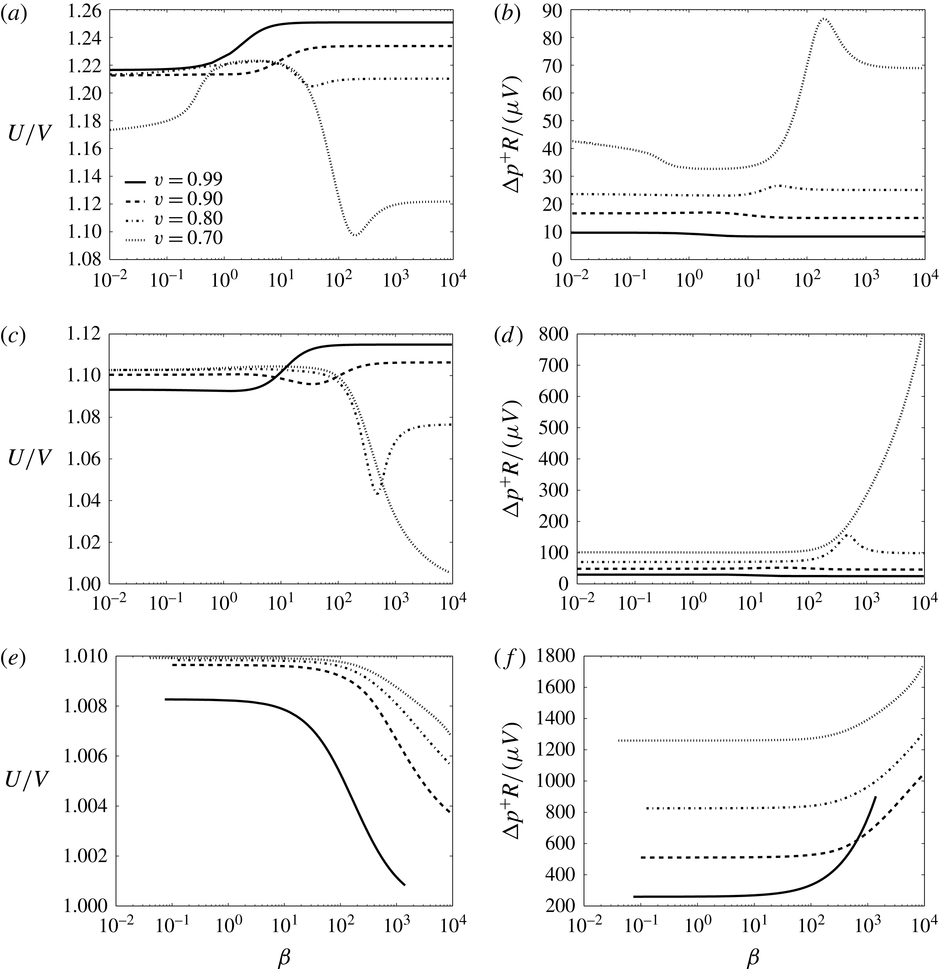
Less has been reported on the hydrodynamics of vesicles in bounded Poiseuille flows, in which particle interactions are screened by the conduit walls to produce an exponentially decaying velocity disturbance (Sonshine & Brenner Reference Sonshine and Brenner1966; Liron & Shahar Reference Liron and Shahar1978). In circular Poiseuille flow with tube radius
 $R$
and suspending medium viscosity
 $\unicode[STIX]{x1D707}$
, a freely suspended vesicle samples only a portion of the velocity field and translates with an axial velocity
 $U$
that is different from the mean fluid velocity
 $V$
in the far field. The relative velocity
 $U/V$
thus measures the vesicle mobility in comparison to the mean flow. The velocity disturbance produced by the suspended vesicle enhances the viscous traction on the tube wall, resulting in a pressure drop
 $\unicode[STIX]{x0394}p^{+}$
in excess of the vesicle-free flow (Brenner Reference Brenner1970). The dimensionless extra pressure drop
 $\unicode[STIX]{x0394}p^{+}R/(\unicode[STIX]{x1D707}V)$
is important, for example, in the determination of the effective viscosity of a vesicle suspension in conduit flow. Since vesicles can deform in response to flow (unlike rigid particles), the dimensionless groups
 $U/V$
and
 $\unicode[STIX]{x0394}p^{+}R/(\unicode[STIX]{x1D707}V)$
are nonlinearly coupled.
To date, the only experimental study of vesicle motion in capillary flow is due to Vitkova, Mader & Podgorski (Reference Vitkova, Mader and Podgorski2004). In their study, the authors reported axisymmetric shapes and measured the effect of capillary confinement on the relative velocity
 $U/V$
. They showed that capillary confinement reduces the mobility, but did not highlight the effect of shape deformation on the mobility nor did they measure the dimensionless extra pressure drop
 $\unicode[STIX]{x0394}p^{+}R/(\unicode[STIX]{x1D707}V)$
. Recent advances in the numerical simulation of vesicles in viscous flows motivates theoretical investigation of bounded vesicle suspensions. Such problems are of the ‘free boundary type’, meaning that the hydrodynamical calculation is coupled to determination of the vesicle shape for a particular flow geometry.
Recently, Barakat & Shaqfeh (Reference Barakat and Shaqfeh2018) developed a rigorous theory using the method of matched asymptotic expansions for the motion of a vesicle in a bounded Poiseuille flow in the limit where the ratio of the vesicle radius to the tube radius
 $\unicode[STIX]{x1D706}=R_{0}/R$
approaches a critical value
 $\unicode[STIX]{x1D706}_{c}$
(here,
 $R_{0}=\sqrt{A_{0}/(4\unicode[STIX]{x03C0})}$
is defined with respect to the vesicle surface area
 $A_{0}$
). The critical radius ratio
 $\unicode[STIX]{x1D706}_{c}$
is related to the vesicle reduced volume
 $\unicode[STIX]{x1D710}=\unicode[STIX]{x1D6FA}_{0}/((4/3)\unicode[STIX]{x03C0}R_{0}^{3})$
(
 $\unicode[STIX]{x1D6FA}_{0}$
being the vesicle volume) by the equation for a spherocylinder,
 $$\begin{eqnarray}2\unicode[STIX]{x1D710}{\unicode[STIX]{x1D706}_{c}}^{3}-3{\unicode[STIX]{x1D706}_{c}}^{2}+1=0.\end{eqnarray}$$
For
 $\unicode[STIX]{x1D706}>\unicode[STIX]{x1D706}_{c}$
, the vesicle cannot pass through the tube cleanly without rupturing. In the limit as
 $\unicode[STIX]{x1D706}\rightarrow \unicode[STIX]{x1D706}_{c}$
, the thin film separating the vesicle membrane from the tube wall becomes vanishingly small compared to the tube radius. The asymptotic theory of Barakat & Shaqfeh (Reference Barakat and Shaqfeh2018) produced the following predictions for the relative velocity
 $U/V$
and dimensionless extra pressure drop
 $\unicode[STIX]{x0394}p^{+}R/(\unicode[STIX]{x1D707}V)$
as
 $\unicode[STIX]{x1D706}\rightarrow \unicode[STIX]{x1D706}_{c}$
(equations (8.8) and (8.9) in their paper):
 $$\begin{eqnarray}\displaystyle & \displaystyle \frac{U}{V}=1+\frac{4}{3}\left(\frac{3\unicode[STIX]{x1D706}_{c}^{2}-2}{4\unicode[STIX]{x1D706}_{c}^{2}-3}\right)\left(1-\frac{\unicode[STIX]{x1D706}}{\unicode[STIX]{x1D706}_{c}}\right)+O\left[\left(1-\frac{\unicode[STIX]{x1D706}}{\unicode[STIX]{x1D706}_{c}}\right)^{2}\right], & \displaystyle\end{eqnarray}$$
 $$\begin{eqnarray}\displaystyle & \displaystyle \frac{\unicode[STIX]{x0394}p^{+}R}{\unicode[STIX]{x1D707}V}=4(\unicode[STIX]{x1D706}_{c}^{2}-1)\left(1-\frac{\unicode[STIX]{x1D706}}{\unicode[STIX]{x1D706}_{c}}\right)^{-1}+\left(\frac{4\sqrt{2}\unicode[STIX]{x03C0}}{4\unicode[STIX]{x1D706}_{c}^{2}-3}\right)\left(1-\frac{\unicode[STIX]{x1D706}}{\unicode[STIX]{x1D706}_{c}}\right)^{-1/2}+O(1). & \displaystyle\end{eqnarray}$$
 $\unicode[STIX]{x1D706}_{c}$
, spanning ‘sphere-like’ vesicles (
 $\unicode[STIX]{x1D706}_{c}=1$
) to ‘spherocylinder-like’ vesicles (
 $\unicode[STIX]{x1D706}_{c}>1$
). The effect of membrane bending elasticity, which can become relevant at low flow rates and for highly aspherical vesicles, is neglected in (1.2). Although the theory of Barakat & Shaqfeh (Reference Barakat and Shaqfeh2018) is asymptotic in the limit
 $\unicode[STIX]{x1D706}/\unicode[STIX]{x1D706}_{c}\rightarrow 1$
, the radius of convergence of the asymptotic series for
 $\unicode[STIX]{x0394}p^{+}R/(\unicode[STIX]{x1D707}V)$
is extremely small due to the stress singularity at maximal confinement. As such, their theory cannot yield quantitative results for the pressure drop when the ratio
 $\unicode[STIX]{x1D706}/\unicode[STIX]{x1D706}_{c}$
is sufficiently less than unity. Although some analytical progress is possible in the opposite limit (
 $\unicode[STIX]{x1D706}/\unicode[STIX]{x1D706}_{c}\rightarrow 0$
) via small-deformation theory (Danker, Vlahovska & Misbah Reference Danker, Vlahovska and Misbah2009; Farutin & Misbah Reference Farutin and Misbah2011), the resulting predictions are limited to nearly spherical vesicles and cannot be used to study a large shape configuration space. Therefore, direct numerical methods are vital to supply accurate predictions in the regime
 $0<\unicode[STIX]{x1D706}/\unicode[STIX]{x1D706}_{c}<1$
.
Unfortunately, the three-dimensional (3D) computation of vesicle motion in conduit flow has proven to be a difficult task, mainly for two reasons. Firstly, vesicles that are suspended in a viscous flow are prone to shape transitions (Kantsler & Steinberg Reference Kantsler and Steinberg2006; Deschamps, Kantsler & Steinberg Reference Deschamps, Kantsler and Steinberg2009; Zhao & Shaqfeh Reference Zhao and Shaqfeh2011; Farutin & Misbah Reference Farutin and Misbah2012) and shape instabilities (Kantsler, Segre & Steinberg Reference Kantsler, Segre and Steinberg2008a ; Zhao & Shaqfeh Reference Zhao and Shaqfeh2013b ; Narsimhan, Spann & Shaqfeh Reference Narsimhan, Spann and Shaqfeh2014, Reference Narsimhan, Spann and Shaqfeh2015) due to nonlinearities associated with vesicle membrane incompressibility. These phenomena are further convoluted by the various numerical instabilities that can arise in a hydrodynamical computation, which are sometimes difficult to differentiate from actual ‘physical instabilities’. Secondly, bounded fluid-flow calculations typically require highly refined grids in order to resolve the hydrodynamic interaction between the vesicle surface and the wall boundary. As a result, these calculations can become computationally expensive. The latter issue is a general facet of all bounded suspension calculations. For example, Janssen et al. (Reference Janssen, Baron, Anderson, Blawzdziewicz, Loewenberg and Wajnryb2012) reported that the collective motion of droplets and rigid particles between two parallel plates could take up to months to resolve (very long residence times) using the boundary element method (BEM). Particle motion in conduit flow represents an even more challenging task due to enhanced particle–wall interactions, which result in an exponential decay of the velocity disturbance as a function of distance from the source. By contrast, the disturbance field in a parallel-plate geometry decays algebraically, as shown by Liron & Mochon (Reference Liron and Mochon1976).
Due to the aforementioned challenges, previous numerical studies on bounded vesicle suspensions have mainly focused on two-dimensional (2D) or axisymmetric geometries, specifically examining morphological (i.e., shape) changes due to confinement. As pointed out in an appendix by Thiebaud & Misbah (Reference Thiebaud and Misbah2013), the velocity disturbance produced in a 2D Poiseuille flow decays exponentially and, therefore, is somewhat analogous to the particle–wall interaction of a particle suspended in 3D circular Poiseuille flow. Kaoui et al. (Reference Kaoui, Tahiri, Biben, Ez-Zahraouy, Benyoussef, Biros and Misbah2011) reported a theoretical phase diagram of shapes for 2D vesicles in bounded channel flow. Although these authors reported some results for 3D vesicles (including evidence for asymmetric shapes), they concluded that the equivalent 3D calculations were ‘too time consuming’ for systematic study. Aouane et al. (Reference Aouane, Farutin, Thiébaud, Benyoussef, Wagner and Misbah2017) examined the hydrodynamic interaction for a pair of vesicles, also focusing on a 2D geometry. Trozzo et al. (Reference Trozzo, Boedec, Leonetti and Jaeger2015) reported axisymmetric Stokes-flow simulations of vesicles in circular tubes, reproducing several of the shapes observed experimentally by Vitkova et al. (Reference Vitkova, Mader and Podgorski2004). Their method relies on the axisymmetric Green’s function of Tözeren (Reference Tözeren1984) and thus does not require discretization of the channel wall. However, in light of the asymmetric shapes reported by Kaoui et al. (Reference Kaoui, Tahiri, Biben, Ez-Zahraouy, Benyoussef, Biros and Misbah2011) and others, it is unclear that the axisymmetric geometry is an accurate reflection of the actual 3D motion of vesicles in tubes.
In the present study, the motion of vesicle trains in a circular tube is simulated using a previously reported Stokes-flow boundary integral equation method (Zhao, Shaqfeh & Narsimhan Reference Zhao, Shaqfeh and Narsimhan2012; Zhao & Shaqfeh Reference Zhao and Shaqfeh2013a ). Although the present work focuses on circular tubes, the numerical method is amenable to conduits of arbitrary cross-section. The principal goal of this study is to examine the influence of the relevant dimensionless parameters on vesicle shape deformation and hydrodynamics in the confined geometry. A periodic arrangement of identical vesicles, initially placed on the channel centreline with uniform spacing in the axial direction, is assumed a priori. This configuration is an idealization of vesicle suspension flow through a conduit. In reality, the suspension configuration will depend on both the concentration and polydispersity of the suspension. Such effects are not the focus of the present work, nor is the stability of the assumed arrangement with respect to fluctuations in concentration.
Under moderate confinement, the numerical simulation technique presented herein accurately and efficiently solves the Stokes-flow problem for a wide variety of conditions. As confinement increases, regions of the fluid film become thin, demanding the use of sufficiently refined meshes to accurately capture the lubrication interaction. 3D numerical simulation techniques become impractical in this regime due to the high computational cost, even with the speedup gained by using fast, matrix-free iterative solvers. It is for this reason that a lubrication theory is also developed herein in order to predict the vesicle motion under high confinement. It is shown that this theory accurately predicts the (most confined) BEM calculations and achieves the correct asymptotic behaviour reported by Barakat & Shaqfeh (Reference Barakat and Shaqfeh2018).
Although the focus of the present work is on the steady-state motion, it is demonstrated herein that the nonlinear evolution of the vesicle shape introduces temporal dynamics and symmetry breaking. These temporal variations in vesicle shape morphology typically result in only minor changes to the relative velocity
 $U/V$
and dimensionless extra pressure drop
 $\unicode[STIX]{x0394}p^{+}R/(\unicode[STIX]{x1D707}V)$
. Consequently, while it is a rather laborious task to systematically map out the long-time dynamics of vesicle shape morphology in conduit flow, it is comparatively easier (and useful) to quantify the hydrodynamics over a wide parameter space with acceptable accuracy. Furthermore, it is shown that when vesicles are highly confined, their motion is steady and well described by lubrication theory.
This paper is organized as follows. In § 2, the governing equations for the Stokes-flow calculation are presented as an initial-boundary-value problem. The numerical method using the boundary integral formulation is discussed in § 3. An axisymmetric lubrication theory is developed in § 4 for a single vesicle. A discussion of the numerical results is presented in § 5. Concluding remarks are given in § 6.
2 Governing equations
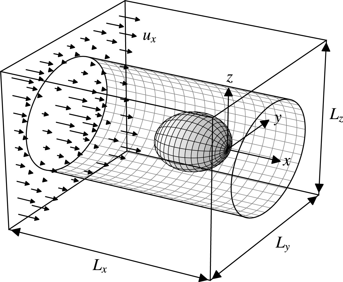
A schematic of the domain is shown in figure 1 with Cartesian axes
 $(x,y,z)=(x_{1},x_{2},x_{3})$
. A periodic train of identical vesicles is placed along the axis of a circular tube of radius
 $R$
. The vesicles are oriented so that their initial configuration at time
 $t=0$
is symmetric about the
 $x$
-axis with spacing
 $L_{x}$
between their centroids (here, the vesicle–vesicle separation distance
 $L_{x}$
supplants the suspension concentration as an independent parameter, due to the assumed configuration). The exterior fluid volume is denoted by
 $\unicode[STIX]{x1D6FA}$
, the interior fluid volume by
 $\unicode[STIX]{x1D6FA}_{0}$
, the wall surface by
 $W$
, and the vesicle surface by
 $M$
.
Schematic of a periodic train of identical vesicles in a circular tube. Only the
 $z=0$
plane is shown. The system is symmetric about the
 $x$
-axis at
 $t=0$
.

In the creeping flow regime, the fluid velocity
 $\boldsymbol{u}$
and stress
 $\unicode[STIX]{x1D64E}$
satisfy the Stokes equations (written below in Einstein notation),
 $$\begin{eqnarray}\displaystyle \left.\begin{array}{@{}c@{}}\displaystyle \frac{\unicode[STIX]{x2202}u_{j}}{\unicode[STIX]{x2202}x_{j}}=0,\\ \displaystyle \frac{\unicode[STIX]{x2202}S_{ij}}{\unicode[STIX]{x2202}x_{j}}=-\frac{\unicode[STIX]{x2202}p}{\unicode[STIX]{x2202}x_{i}}+\unicode[STIX]{x1D707}\unicode[STIX]{x1D6FB}^{2}u_{i}=0,\end{array}\right\}\quad \boldsymbol{x}\in \unicode[STIX]{x1D6FA}\backslash \unicode[STIX]{x1D6FA}_{0}, & & \displaystyle\end{eqnarray}$$
 $$\begin{eqnarray}\displaystyle \left.\begin{array}{@{}c@{}}\displaystyle \frac{\unicode[STIX]{x2202}u_{j}}{\unicode[STIX]{x2202}x_{j}}=0,\\ \displaystyle \frac{\unicode[STIX]{x2202}S_{ij}}{\unicode[STIX]{x2202}x_{j}}=-\frac{\unicode[STIX]{x2202}p}{\unicode[STIX]{x2202}x_{i}}+\hat{\unicode[STIX]{x1D707}}\unicode[STIX]{x1D6FB}^{2}u_{i}=0,\end{array}\right\}\quad \boldsymbol{x}\in \unicode[STIX]{x1D6FA}_{0}, & & \displaystyle\end{eqnarray}$$
 $\unicode[STIX]{x1D707}$
is the exterior fluid viscosity,
 $\hat{\unicode[STIX]{x1D707}}$
is the interior fluid viscosity and
 $p$
is the fluid pressure (a Lagrange field that enforces volume incompressibility). On the tube wall, the velocity
 $\boldsymbol{u}$
is subject to the ‘no-slip condition’,
 $$\begin{eqnarray}u_{i}=0,\quad \boldsymbol{x}\in W.\end{eqnarray}$$
The vesicle train is forced into motion by a mean flow:
 $$\begin{eqnarray}\displaystyle & \displaystyle u_{i}=\langle u_{i}\rangle +u_{pi},\quad \langle u_{pi}\rangle =0, & \displaystyle\end{eqnarray}$$
 $$\begin{eqnarray}\displaystyle & \displaystyle S_{ij}=-x_{k}\left\langle \frac{\unicode[STIX]{x2202}p}{\unicode[STIX]{x2202}x_{k}}\right\rangle \unicode[STIX]{x1D6FF}_{ij}+S_{pij},\quad \langle S_{pij}\rangle =0, & \displaystyle\end{eqnarray}$$
where
 $\boldsymbol{u}_{p}$
and
 $\unicode[STIX]{x1D64E}_{p}$
are periodic and
 $\langle \,\cdot \,\rangle \equiv (1/\unicode[STIX]{x1D6FA}_{p})\int _{\unicode[STIX]{x1D6FA}_{p}}(\,\cdot \,)\,\text{d}^{3}\boldsymbol{x}$
denotes the appropriate average over a periodic volume
 $\unicode[STIX]{x1D6FA}_{p}$
. The volume-averaged velocity
 $\langle \boldsymbol{u}\rangle$
is specified a priori, with the average pressure gradient
 $\langle \unicode[STIX]{x1D735}p\rangle$
uniquely determined by a force balance (Zhao et al.
Reference Zhao, Isfahani, Olson and Freund2010),
 $$\begin{eqnarray}\left\langle \frac{\unicode[STIX]{x2202}p}{\unicode[STIX]{x2202}x_{i}}\right\rangle =-\frac{1}{\unicode[STIX]{x1D6FA}_{p}}\int _{W}f_{i}\,\text{d}S(\boldsymbol{x}),\end{eqnarray}$$
where
 $\boldsymbol{f}=\unicode[STIX]{x1D64E}\boldsymbol{\cdot }\boldsymbol{n}$
is the fluid traction and
 $\boldsymbol{n}$
is the unit normal of the surface. The imposed mean flow results in a mean tube velocity,
 $$\begin{eqnarray}V=\frac{1}{\unicode[STIX]{x03C0}R^{2}}\int _{S}u_{1}\,\text{d}S(\boldsymbol{x}),\end{eqnarray}$$
where
 $S$
denotes a tube cross-sectional surface of constant
 $x$
. The (axial component of the) translational velocity of any vesicle in the train is given by,
 $$\begin{eqnarray}\displaystyle U & = & \displaystyle \frac{1}{\unicode[STIX]{x1D6FA}_{0}}\int _{\unicode[STIX]{x1D6FA}_{0}}u_{1}\,\text{d}^{3}\boldsymbol{x},\nonumber\\ \displaystyle & = & \displaystyle \frac{1}{\unicode[STIX]{x1D6FA}_{0}}\int _{M}x_{1}u_{i}n_{i}\,\text{d}S(\boldsymbol{x}),\end{eqnarray}$$
where to the second line the divergence theorem and the continuity condition have been applied. Here,
 $\unicode[STIX]{x1D6FA}_{0}$
denotes the vesicle volume.
The vesicle membrane is treated as an internally fluid, incompressible surface with a bending stiffness
 $B$
. The bending energy of the bilayer governed by the Helfrich energy functional (Helfrich Reference Helfrich1973),
 $$\begin{eqnarray}E=2B\int _{M}H^{2}\,\text{d}S(\boldsymbol{x}),\end{eqnarray}$$
where
 $H$
is the mean curvature. By applying the principle of virtual work to (2.8) (subject to the constraint that membrane surface area be conserved locally), one derives the membrane force density that balances the net traction exerted on the membrane by the bulk fluids (Jenkins Reference Jenkins1977; Zhong-can & Helfrich Reference Zhong-can and Helfrich1989). Thus, the jump conditions for
 $\boldsymbol{u}$
and
 $\unicode[STIX]{x1D64E}$
on
 $M$
are found to be
 $$\begin{eqnarray}\left.\begin{array}{@{}c@{}}\unicode[STIX]{x27E6}u_{i}\unicode[STIX]{x27E7}=0,\\ \displaystyle n_{i}\unicode[STIX]{x27E6}f_{i}\unicode[STIX]{x27E7}=-2H\unicode[STIX]{x1D70F}+2B\left[P_{ij}\frac{\unicode[STIX]{x2202}}{\unicode[STIX]{x2202}x_{j}}\left(P_{ik}\frac{\unicode[STIX]{x2202}H}{\unicode[STIX]{x2202}x_{k}}\right)+2(H^{2}-K)H\right],\\ \displaystyle P_{ij}\unicode[STIX]{x27E6}f_{j}\unicode[STIX]{x27E7}=-P_{ij}\frac{\unicode[STIX]{x2202}\unicode[STIX]{x1D70F}}{\unicode[STIX]{x2202}x_{j}},\end{array}\right\}\quad \boldsymbol{x}\in M,\end{eqnarray}$$
where
 $\unicode[STIX]{x27E6}\,\cdot \,\unicode[STIX]{x27E7}$
is the ‘jump’ operator,
 $\unicode[STIX]{x1D64B}=\unicode[STIX]{x1D644}-\boldsymbol{n}\boldsymbol{n}$
is the surface projection tensor,
 $K$
is the Gaussian curvature, and
 $\unicode[STIX]{x1D70F}$
is the membrane tension (a Lagrange field that enforces surface-area incompressibility on
 $M$
). The curvature invariants
 $H$
and
 $K$
are related to
 $\boldsymbol{n}$
by the relations
 $$\begin{eqnarray}2H=-\frac{\unicode[STIX]{x2202}n_{j}}{\unicode[STIX]{x2202}x_{j}},\quad 2K=\frac{\unicode[STIX]{x2202}n_{i}}{\unicode[STIX]{x2202}x_{j}}\frac{\unicode[STIX]{x2202}n_{j}}{\unicode[STIX]{x2202}x_{i}}-\left(\frac{\unicode[STIX]{x2202}n_{j}}{\unicode[STIX]{x2202}x_{j}}\right)^{2},\quad \boldsymbol{x}\in M.\end{eqnarray}$$
Just as the fluid pressure
 $p$
guarantees satisfaction of the incompressibility conditions in the bulk fluid (requiring that
 $\boldsymbol{u}$
be solenoidal), the membrane tension
 $\unicode[STIX]{x1D70F}$
enforces the surface incompressibility condition,
 $$\begin{eqnarray}P_{ij}\frac{\unicode[STIX]{x2202}u_{i}}{\unicode[STIX]{x2202}x_{j}}=0,\quad \boldsymbol{x}\in M.\end{eqnarray}$$
This equation stipulates that
 $\boldsymbol{u}$
be solenoidal (in the two-dimensional sense) on
 $M$
.
Since
 $M$
is a free surface, the kinematic condition further requires that the membrane translate with the local fluid velocity,
 $$\begin{eqnarray}\frac{\text{D}x_{si}}{\text{D}t}=\frac{\unicode[STIX]{x2202}x_{si}}{\unicode[STIX]{x2202}t}+u_{j}\frac{\unicode[STIX]{x2202}x_{si}}{\unicode[STIX]{x2202}x_{j}}=u_{i},\quad \boldsymbol{x}\in M,\end{eqnarray}$$
where
 $\text{D}/\text{D}t$
is the material derivative and
 $\boldsymbol{x}_{s}$
denotes the position of a point on the membrane. The unit normal
 $\boldsymbol{n}$
can be related to
 $\boldsymbol{x}_{s}$
via standard relations from differential geometry (Kreyszig Reference Kreyszig1959).
Although the governing Stokes equations are steady, the boundary-value problem is time-dependent through the kinematic condition (2.12). Thus, the system is evolved starting from some initial configuration for the vesicle shape. At the initial time point, the total vesicle volume
 $\unicode[STIX]{x1D6FA}_{0}$
and surface area
 $A_{0}$
are prescribed:
 $$\begin{eqnarray}\text{at}~t=0:\quad \int _{\unicode[STIX]{x1D6FA}_{0}}\text{d}^{3}\boldsymbol{x}=\unicode[STIX]{x1D6FA}_{0},\quad \int _{\unicode[STIX]{x2202}\unicode[STIX]{x1D6FA}_{0}}\,\text{d}S=A_{0}.\end{eqnarray}$$
Thus,
 $\unicode[STIX]{x1D6FA}_{0}$
and
 $A_{0}$
take the role of parameters in the initial-boundary-value problem. Surface-area- and volume-incompressibility require that
 $\unicode[STIX]{x1D6FA}_{0}$
and
 $A_{0}$
be time-invariant in the Lagrangian sense,
 $$\begin{eqnarray}\frac{\text{D}\unicode[STIX]{x1D6FA}_{0}}{\text{D}t}=0,\quad \frac{\text{D}A_{0}}{\text{D}t}=0.\end{eqnarray}$$
To recast the problem in dimensionless form, all length scales are rendered dimensionless by
 $R$
, fluid velocity
 $\boldsymbol{u}$
by
 $V$
, fluid pressure
 $p$
by
 $\unicode[STIX]{x1D707}V/R$
, and membrane tension
 $\unicode[STIX]{x1D70F}$
by
 $\unicode[STIX]{x1D707}V$
. The solution for these fields is parametrized by five dimensionless groups: the viscosity ratio
 $\unicode[STIX]{x1D705}=\hat{\unicode[STIX]{x1D707}}/\unicode[STIX]{x1D707}$
, bending parameter
 $\unicode[STIX]{x1D6FD}=B/(\unicode[STIX]{x1D707}VR^{2})$
, radius ratio
 $\unicode[STIX]{x1D706}=R_{0}/R$
, reduced volume
 $\unicode[STIX]{x1D710}=\unicode[STIX]{x1D6FA}_{0}/((4/3)\unicode[STIX]{x03C0}R_{0}^{3})$
, and the vesicle–vesicle separation parameter
 $\unicode[STIX]{x1D6FF}=L_{x}/R$
. Here,
 $R_{0}=\sqrt{A_{0}/(4\unicode[STIX]{x03C0})}$
is the effective vesicle radius based on surface area.
3 Boundary element method (BEM)
The Stokes-flow problem described in § 2 is solved using a previously reported boundary integral equation method (Zhao et al.
Reference Zhao, Shaqfeh and Narsimhan2012; Zhao & Shaqfeh Reference Zhao and Shaqfeh2013a
). A summary of the method is outlined below. First, by use of Green’s theorem, the fluid velocity inside a test volume
 $\unicode[STIX]{x1D6FA}^{\ast }$
can be represented by a convolution of point forces and point force dipoles distributed over the bounding surface
 $\unicode[STIX]{x2202}\unicode[STIX]{x1D6FA}^{\ast }$
(Pozrikidis Reference Pozrikidis1992):
 $$\begin{eqnarray}\displaystyle & & \displaystyle -\frac{1}{8\unicode[STIX]{x03C0}\unicode[STIX]{x1D707}}\int _{\unicode[STIX]{x2202}\unicode[STIX]{x1D6FA}^{\ast }}f_{i}(\boldsymbol{x})G_{ij}(\boldsymbol{x},\boldsymbol{x}_{0})\,\text{d}S(\boldsymbol{x})+\frac{1}{8\unicode[STIX]{x03C0}}\int _{\unicode[STIX]{x2202}\unicode[STIX]{x1D6FA}^{\ast }}u_{i}(\boldsymbol{x})T_{ijk}(\boldsymbol{x},\boldsymbol{x}_{0})n_{k}(\boldsymbol{x})\,\text{d}S(\boldsymbol{x})\nonumber\\ \displaystyle & & \displaystyle \quad =\left\{\begin{array}{@{}ll@{}}0,\quad & \boldsymbol{x}_{0}\not \in \unicode[STIX]{x1D6FA}^{\ast },\\ u_{j}(\boldsymbol{x}_{0}),\quad & \boldsymbol{x}_{0}\in \unicode[STIX]{x1D6FA}^{\ast }\backslash \unicode[STIX]{x2202}\unicode[STIX]{x1D6FA}^{\ast },\\ {\textstyle \frac{1}{2}}K_{jk}(\boldsymbol{x}_{0})u_{k}(\boldsymbol{x}_{0}),\quad & \boldsymbol{x}_{0}\in \unicode[STIX]{x2202}\unicode[STIX]{x1D6FA}^{\ast },\end{array}\right.\end{eqnarray}$$
where
 $\unicode[STIX]{x1D642}$
and
 $\unicode[STIX]{x1D64F}$
are the Green’s functions of Hasimoto (Reference Hasimoto1959) and
 $\unicode[STIX]{x1D646}$
is the principal-value tensor. (If the field point
 $\boldsymbol{x}_{0}$
lies on a Lyapunov smooth surface, then
 $\unicode[STIX]{x1D646}=\unicode[STIX]{x1D644}$
.) The Green’s functions
 $\unicode[STIX]{x1D642}$
and
 $\unicode[STIX]{x1D64F}$
are periodic in the
 $x$
,
 $y$
and
 $z$
directions with the lattice vector
 $\boldsymbol{L}=(L_{x},L_{y},L_{z})$
, as shown in figure 2. Since the tube wall is a no-slip surface, the addition of periodic boundary conditions in the
 $y$
and
 $z$
directions is inconsequential to the flow field inside the tube so long as
 $L_{y}>R$
and
 $L_{z}>R$
. (Verification tests were performed to ensure that the numerical results were insensitive to the box dimensions in the
 $y$
and
 $z$
directions.) Numerically, there is an advantage to using fully periodic boundary conditions in that the Green’s functions may be rapidly computed by use of the smooth particle mesh Ewald (SPME) algorithm (Saintillan, Darve & Shaqfeh Reference Saintillan, Darve and Shaqfeh2005; Zhao et al.
Reference Zhao, Isfahani, Olson and Freund2010).
Schematic of the basic cell used in the 3D BEM simulations. The cell is periodically replicated in the
 $x$
,
 $y$
and
 $z$
directions.

By taking the limit as the field point
 $\boldsymbol{x}_{0}$
approaches the boundary points
 $\boldsymbol{x}_{0}^{M}\in M$
and
 $\boldsymbol{x}_{0}^{W}\in W$
, a system of boundary integral equations for the membrane velocity
 $\boldsymbol{u}^{M}=\boldsymbol{u}(\boldsymbol{x}\in M)$
and wall traction jump
 $\boldsymbol{f}^{W}=\unicode[STIX]{x27E6}\,\boldsymbol{f}(\boldsymbol{x}\in W)\unicode[STIX]{x27E7}$
may be derived from (3.1). The result, expressed in matrix-vector form, is
 $$\begin{eqnarray}\left[\begin{array}{@{}cc@{}}\displaystyle \int _{M}A_{ij}(\boldsymbol{x},\boldsymbol{x}_{0}^{M}) & \displaystyle \int _{W}B_{ij}(\boldsymbol{x},\boldsymbol{x}_{0}^{M})\\ \displaystyle \int _{M}C_{ij}(\boldsymbol{x},\boldsymbol{x}_{0}^{W}) & \displaystyle \int _{W}D_{ij}(\boldsymbol{x},\boldsymbol{x}_{0}^{W})\end{array}\right]\left[\begin{array}{@{}c@{}}u_{i}^{M}(\boldsymbol{x})\\ \,f_{i}^{W}(\boldsymbol{x})\end{array}\right]\text{d}S(\boldsymbol{x})=\left[\begin{array}{@{}c@{}}b_{j}(\boldsymbol{x}_{0}^{M})\\ b_{j}(\boldsymbol{x}_{0}^{W})\end{array}\right],\end{eqnarray}$$
where
 $$\begin{eqnarray}\displaystyle & \displaystyle A_{ij}(\boldsymbol{x},\boldsymbol{x}_{0})=\frac{1+\unicode[STIX]{x1D705}}{2}\unicode[STIX]{x1D6FF}(\boldsymbol{x}-\boldsymbol{x}_{0})K_{ij}(\boldsymbol{x})-\frac{1-\unicode[STIX]{x1D705}}{8\unicode[STIX]{x03C0}}T_{ijk}(\boldsymbol{x},\boldsymbol{x}_{0})n_{k}(\boldsymbol{x}), & \displaystyle\end{eqnarray}$$
 $$\begin{eqnarray}\displaystyle & \displaystyle B_{ij}(\boldsymbol{x},\boldsymbol{x}_{0})=\frac{1}{8\unicode[STIX]{x03C0}\unicode[STIX]{x1D707}}G_{ij}(\boldsymbol{x},\boldsymbol{x}_{0}), & \displaystyle\end{eqnarray}$$
 $$\begin{eqnarray}\displaystyle & \displaystyle C_{ij}(\boldsymbol{x},\boldsymbol{x}_{0})=-\frac{1-\unicode[STIX]{x1D705}}{8\unicode[STIX]{x03C0}}T_{ijk}(\boldsymbol{x},\boldsymbol{x}_{0})n_{k}(\boldsymbol{x}), & \displaystyle\end{eqnarray}$$
 $$\begin{eqnarray}\displaystyle & \displaystyle D_{ij}(\boldsymbol{x},\boldsymbol{x}_{0})=\frac{1}{8\unicode[STIX]{x03C0}\unicode[STIX]{x1D707}}G_{ij}(\boldsymbol{x},\boldsymbol{x}_{0}) & \displaystyle\end{eqnarray}$$
are the kernels and
 $$\begin{eqnarray}b_{j}(\boldsymbol{x}_{0})=-\frac{1}{8\unicode[STIX]{x03C0}\unicode[STIX]{x1D707}}\int _{M}f_{i}^{M}(\boldsymbol{x})G_{ij}(\boldsymbol{x},\boldsymbol{x}_{0})\,\text{d}S(\boldsymbol{x})+\langle u_{j}\rangle\end{eqnarray}$$
is the source. Here,
 $\boldsymbol{f}^{M}=\unicode[STIX]{x27E6}\,\boldsymbol{f}(\boldsymbol{x}\in M)\unicode[STIX]{x27E7}$
is the membrane traction jump. The volume-averaged velocity
 $\langle \boldsymbol{u}\rangle$
naturally appears in the source as a direct consequence of applying the divergence theorem to the surface integrals over the bounding surface of the periodic cell.
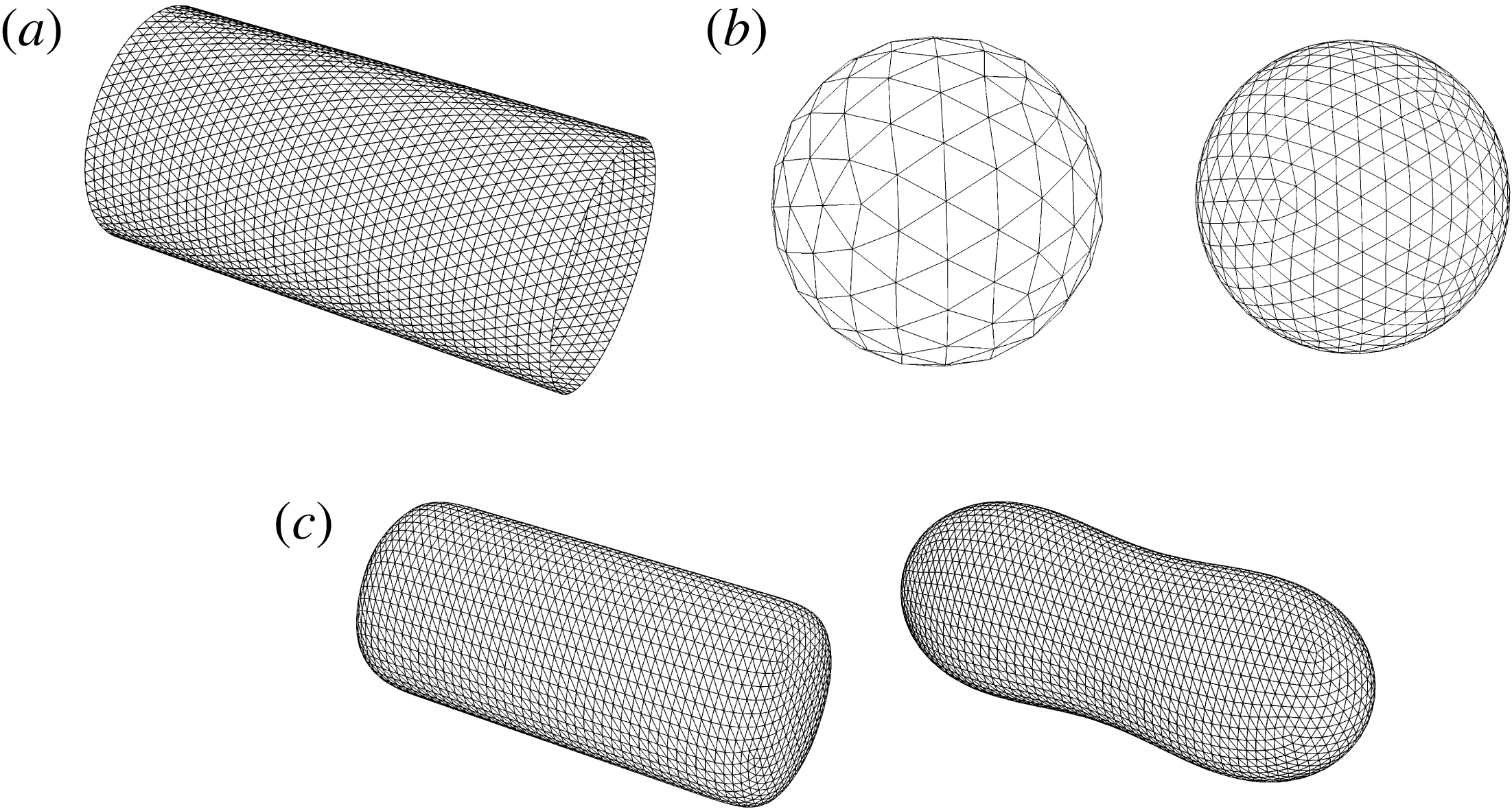
Unstructured meshes. (a) Tube wall surface
 $W$
of length
 $L_{x}=4R$
discretized into
 $N^{W}=5\,796$
triangular elements. (b) Vesicle surface
 $M$
discretized into
 $N^{M}=162$
(left) and 642 (right) triangular elements by successively subdividing an icosahedron four and eight times, respectively. This type of mesh is appropriate if the reduced volume
 $\unicode[STIX]{x1D710}$
is close to unity. (c) Vesicle surface
 $M$
discretized into
 $N^{M}=5\,376$
triangular elements by first Loop subdividing a cylindrical surface (left) and subsequently relaxing the mesh in a Stokes-flow BEM simulation with
 $\langle \boldsymbol{u}\rangle =\mathbf{0}$
(right). This type of mesh is appropriate if the reduced volume
 $\unicode[STIX]{x1D710}$
is far from unity.

The boundary integral equations (3.2) are solved for the membrane velocity
 $\boldsymbol{u}^{M}$
and wall traction jump
 $\boldsymbol{f}^{W}$
via the collocation method (Youngren & Acrivos Reference Youngren and Acrivos1975; Pozrikidis Reference Pozrikidis1992). Collocation points are placed at the vertices of unstructured, triangulated meshes approximating the surfaces
 $M$
and
 $W$
. Some of the unstructured meshes used in the presently reported simulations are shown in figure 3. The wall mesh is discretized into
 $N^{W}$
equally sized triangles. The vesicle mesh is discretized into
 $N^{M}$
triangles either by successive subdivision of an icosahedron (appropriate for nearly spherical vesicles, for which the reduced volume
 $\unicode[STIX]{x1D710}$
is close to unity) or by Loop subdivision of a cylindrical surface and subsequent mesh relaxation in a Stokes-flow simulation (for ‘deflated’ vesicles of reduced volume
 $\unicode[STIX]{x1D710}<1$
). The smooth subdivision method of Loop (Reference Loop1987) allows for high-fidelity calculation of membrane curvature for vesicles that are highly aspherical, which is necessary in order to accurately compute the membrane traction jump
 $\boldsymbol{f}^{M}$
(Spann, Zhao & Shaqfeh Reference Spann, Zhao and Shaqfeh2014). The latter is evaluated by a virtual work principle – i.e., by discretely evaluating the variational derivative of (2.8) with respect to a virtual displacement – as described in the appendix of Zhao et al. (Reference Zhao, Spann and Shaqfeh2011).
The unknown density fields
 $\boldsymbol{u}^{M}$
and
 $\boldsymbol{f}^{W}$
are approximated by piecewise linear interpolants on the discretized surfaces
 $M$
and
 $W$
, respectively. The Green’s functions
 $\unicode[STIX]{x1D642}$
and
 $\unicode[STIX]{x1D64F}$
are evaluated by the SPME method using a commercially available fast Fourier transform package. Numerical integration was carried out using a standard three-point quadrature (for regular kernels) or Duffy quadrature (for singular kernels) (Duffy Reference Duffy1982). The discrete form of (3.2) (evaluated at the mesh vertices) is then solved using a matrix-free generalized minimal residual (GMRES) solver on distributed memory parallel computer architectures.
The membrane tension
 $\unicode[STIX]{x1D70F}$
is determined by satisfying (2.11), which requires that the area of a local surface patch on
 $M$
remain time-invariant in the Lagrangian sense. Owing to numerical errors, the instantaneous membrane surface area
 $A_{0}^{\ast }$
will evolve over time and is in general not exactly equal to the target value
 $A_{0}$
(Zhao & Shaqfeh Reference Zhao and Shaqfeh2013b
). The error in the total surface area is controlled by adding a source term
 $\dot{\unicode[STIX]{x1D700}}_{area}=(A_{0}/A_{0}^{\ast }-1)/t_{relax}$
to the right-hand side of (2.11),
 $$\begin{eqnarray}P_{ij}\frac{\unicode[STIX]{x2202}u_{i}^{M}}{\unicode[STIX]{x2202}x_{j}}=\dot{\unicode[STIX]{x1D700}}_{area},\end{eqnarray}$$
where
 $t_{relax}$
is a relaxation time chosen to control the relative change in surface area. If
 $A_{0}^{\ast }=A_{0}$
, then
 $\dot{\unicode[STIX]{x1D700}}_{area}=0$
and the membrane velocity
 $\boldsymbol{u}^{M}$
is divergence-free (in the two-dimensional sense) on
 $M$
. A predictor–corrector method is used to update the membrane velocity
 $\boldsymbol{u}^{M}$
and tension
 $\unicode[STIX]{x1D70F}$
such that (3.2) and (3.8) are both satisfied (Zhao et al.
Reference Zhao, Spann and Shaqfeh2011; Zhao & Shaqfeh Reference Zhao and Shaqfeh2013a
). The bending contribution to the membrane traction jump
 $\boldsymbol{f}^{M}$
is computed implicitly via finite differences during the prediction step in order to preserve numerical stability (Knoll & Keys Reference Knoll and Keys2004). In all of the simulations reported herein, the relative error
 $|A_{0}/A_{0}^{\ast }-1|$
was constrained to within
 $10^{-4}$
by using
 $t_{relax}V/R=1$
.
Once a converged solution of (3.2)–(3.8) is obtained, the Lagrangian surface mesh is evolved in time using the discrete form of the kinematic condition (2.12). To formulate the right-hand side of (2.12), the vesicle translational velocity
 $\boldsymbol{U}$
is first subtracted from the membrane velocity
 $\boldsymbol{u}^{M}$
and the difference is subsequently projected into the local normal and tangent of each vertex. The tangential components of
 $\boldsymbol{u}^{M}$
are adjusted by a mesh relaxation velocity
 $\boldsymbol{v}$
in order to correct local distortion of the mesh elements due to in-plane shear, à la Loewenberg & Hinch (Reference Loewenberg and Hinch1996). This adjustment is necessary to keep a close-to-uniform distribution of vertices in the surface mesh. Thus, (2.12) is modified to read,
 $$\begin{eqnarray}\frac{\text{D}x_{si}}{\text{D}t}=U_{i}+n_{i}n_{j}(u_{j}^{M}-U_{j})+P_{ij}(u_{j}^{M}-U_{j}+v_{j}).\end{eqnarray}$$
The surface positions
 $\boldsymbol{x}_{s}$
are advected using forward Euler timestepping. After the surface is advanced in time, the mesh points are adjusted so that the instantaneous vesicle volume
 $\unicode[STIX]{x1D6FA}_{0}^{\ast }$
does not change by more than 1 %. In practice, the relative error
 $|\unicode[STIX]{x1D6FA}_{0}/\unicode[STIX]{x1D6FA}_{0}^{\ast }-1|$
is negligibly small.
Additional mesh control procedures, such as re-meshing or edge-swapping, were found to be unnecessary to preserve a high-quality mesh for the results shown herein. Numerical instabilities can develop in regions of high curvature (as is common for ‘weakly confined’ vesicles at low reduced volumes
 $\unicode[STIX]{x1D710}\lesssim 0.85$
) if the bending parameter
 $\unicode[STIX]{x1D6FD}$
is small. In such cases, it is necessary to maintain a sufficient number of mesh points in regions of high curvature in order to stabilize high-wavenumber shape fluctuations.
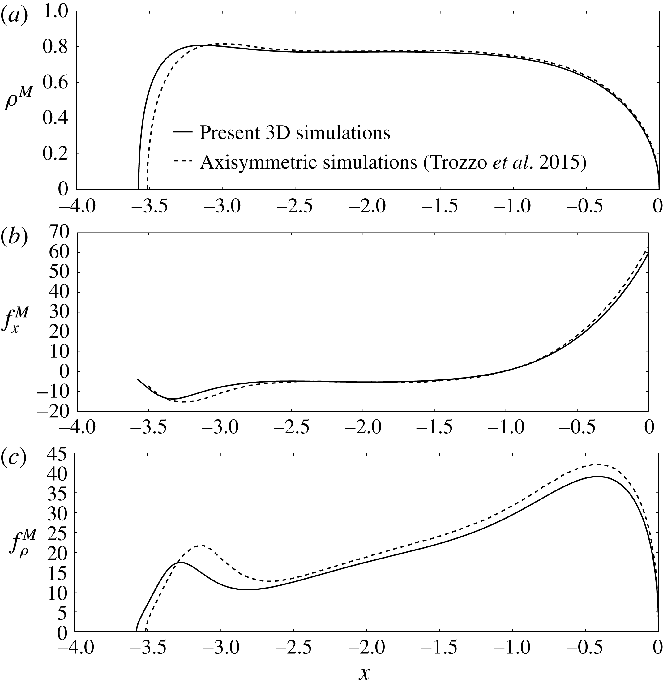
Comparison of the present 3D BEM simulations with the axisymmetric BEM simulations of Trozzo et al. (Reference Trozzo, Boedec, Leonetti and Jaeger2015), figure 15(a) (
 $\unicode[STIX]{x1D710}=0.84$
,
 $\unicode[STIX]{x1D706}=1.2$
,
 $\unicode[STIX]{x1D6FD}=0.01$
,
 $\unicode[STIX]{x1D705}=1$
,
 $\unicode[STIX]{x1D6FF}=10$
). (a) Membrane radius
 $\unicode[STIX]{x1D70C}^{M}=\sqrt{y^{2}+z^{2}}$
. (b) Axial membrane traction jump
 $f_{x}^{M}$
. (c) Radial membrane traction jump
 $f_{\unicode[STIX]{x1D70C}}^{M}$
.

The extra pressure drop is computed as
 $\unicode[STIX]{x0394}p^{+}=-\langle \unicode[STIX]{x2202}p/\unicode[STIX]{x2202}x\rangle /(L_{y}L_{z})-8\unicode[STIX]{x1D707}VL_{x}/R^{2}$
. The vesicle translational velocity
 $U$
is obtained by evaluating the first moment of the normal velocity distribution over the discretized vesicle surface
 $M$
and taking the axial component (cf. (2.7)). In the simulation, the volume-averaged velocity
 $\langle \boldsymbol{u}\rangle$
is prescribed and the mean channel velocity
 $V$
is obtained by assigning ‘probes’ over a channel cross-sectional surface of constant
 $x$
and subsequently performing the weighted average of the axial velocity distribution over that surface (cf. (2.6)). Since
 $\langle \boldsymbol{u}\rangle$
is prescribed in the simulation (rather than the mean velocity
 $V$
), one has to adjust
 $\langle \boldsymbol{u}\rangle$
at each time step in order to maintain
 $V$
at a steady value.
The present 3D BEM simulations were compared to the axisymmetric simulations of Trozzo et al. (Reference Trozzo, Boedec, Leonetti and Jaeger2015) in order to verify that the vesicle shape and membrane traction jump
 $\boldsymbol{f}^{M}$
are accurately resolved. The comparison in figure 4 shows excellent agreement. The slight discrepancy between the two simulations is due to aforementioned numerical errors in discretely satisfying surface-area incompressibility at each time step. Additional numerical experiments (not shown) were conducted in order to ensure that the relative velocity
 $U/V$
and dimensionless extra pressure drop
 $\unicode[STIX]{x0394}p^{+}R/(\unicode[STIX]{x1D707}V)$
were accurately computed using previously reported results for trains of rigid spheres in circular tubes (Wang & Skalak Reference Wang and Skalak1969).
4 Axisymmetric lubrication theory
The boundary integral equations (3.2) become numerically stiff when the gap thickness separating the vesicle membrane and the tube wall becomes small. The high number of mesh elements
 $N^{M}$
and
 $N^{W}$
required to accurately resolve the fluid flow in the thin gap renders the full simulation method computationally expensive due to the density of the BEM matrix. Recently, Barakat & Shaqfeh (Reference Barakat and Shaqfeh2018) developed a small-gap theory for the motion of a single vesicle in a circular tube for
 $(1-\unicode[STIX]{x1D706}/\unicode[STIX]{x1D706}_{c})\ll 1$
, in view of the computational difficulties encountered in this regime. Unfortunately, the radius of convergence for their perturbative solution is very small, owing to the singular nature of the limit
 $\unicode[STIX]{x1D706}/\unicode[STIX]{x1D706}_{c}\rightarrow 1$
.
An alternative approach, which was used by Secomb et al. (Reference Secomb, Skalak, Oozkaya and Gross1986) to study red blood cells in capillary flow, is to assume that the fluid flow near the vesicle surface is steady, axisymmetric, and nearly parallel, the latter of which implies that all velocity components transverse to the flow axis can be neglected (and in turn all velocity gradients along the flow axis are vanishingly small). This approximation is appropriate if the gap thickness is small relative to the vesicle length
 $L$
(but not necessarily small relative to the channel radius
 $R$
). Under conditions of axisymmetry, the surface position vector
 $\boldsymbol{x}_{s}$
has the Eulerian representation,
 $$\begin{eqnarray}x_{si}(\unicode[STIX]{x1D719},x)=x\unicode[STIX]{x1D6FF}_{1i}+\unicode[STIX]{x1D70C}_{s}(x)\cos \unicode[STIX]{x1D719}\,\unicode[STIX]{x1D6FF}_{2i}+\unicode[STIX]{x1D70C}_{s}(x)\sin \unicode[STIX]{x1D719}\,\unicode[STIX]{x1D6FF}_{3i},\end{eqnarray}$$
where
 $\unicode[STIX]{x1D70C}=\sqrt{y^{2}+z^{2}}$
is the radius of a cylinder,
 $\unicode[STIX]{x1D719}=\arctan (z/y)$
is the azimuthal angle, and
 $\unicode[STIX]{x1D70C}=\unicode[STIX]{x1D70C}_{s}(x)\equiv \unicode[STIX]{x1D70C}^{M}$
defines the location of the vesicle membrane in space. The curvature invariants
 $H$
and
 $K$
can be written entirely in terms of
 $\unicode[STIX]{x1D70C}_{s}(x)$
and its derivatives:
 $$\begin{eqnarray}2H=\frac{\unicode[STIX]{x1D70C}_{s}^{3}}{G_{s}^{3}}\frac{\text{d}^{2}\unicode[STIX]{x1D70C}_{s}}{\text{d}x^{2}}-\frac{1}{G_{s}},\quad K=-\frac{\unicode[STIX]{x1D70C}_{s}^{3}}{G_{s}^{4}}\frac{\text{d}^{2}\unicode[STIX]{x1D70C}_{s}}{\text{d}x^{2}},\end{eqnarray}$$
where
 $G_{s}=\unicode[STIX]{x1D70C}_{s}\sqrt{1+(\text{d}\unicode[STIX]{x1D70C}_{s}/\text{d}x)^{2}}$
is the surface metric.
Due to the assumed symmetry, the only admissible solution of (2.11) is a uniform velocity on the membrane. Hence, the vesicle behaves like a rigid body with velocity
 $U$
whose shape must be determined from the membrane stress condition. In the lubrication approximation, the axial velocity field
 $u_{x}$
is governed by the boundary-value problem,
 $$\begin{eqnarray}\frac{1}{\unicode[STIX]{x1D70C}}\frac{\unicode[STIX]{x2202}}{\unicode[STIX]{x2202}\unicode[STIX]{x1D70C}}\left(\unicode[STIX]{x1D70C}\frac{\unicode[STIX]{x2202}u_{x}}{\unicode[STIX]{x2202}\unicode[STIX]{x1D70C}}\right)=\frac{1}{\unicode[STIX]{x1D707}}\frac{\text{d}p}{\text{d}x},\end{eqnarray}$$
 $$\begin{eqnarray}\displaystyle & u_{x}=0\quad \text{at}~\unicode[STIX]{x1D70C}=R, & \displaystyle\end{eqnarray}$$
 $$\begin{eqnarray}\displaystyle & u_{x}=U\quad \text{at}~\unicode[STIX]{x1D70C}=\unicode[STIX]{x1D70C}_{s}(x), & \displaystyle\end{eqnarray}$$
 $$\begin{eqnarray}\int _{\unicode[STIX]{x1D70C}_{s}(x)}^{R}2\unicode[STIX]{x03C0}\unicode[STIX]{x1D70C}(u_{x}-U)\,\text{d}\unicode[STIX]{x1D70C}=\unicode[STIX]{x03C0}R^{2}(V-U).\end{eqnarray}$$
Here, the axial velocity
 $u_{x}$
depends parametrically on
 $x$
only through variations in the membrane shape
 $\unicode[STIX]{x1D70C}_{s}(x)$
. Variations in
 $p$
with respect to
 $\unicode[STIX]{x1D70C}$
are also neglected. Equations (4.3)–(4.5) may be directly solved to yield the Reynolds lubrication equation (Hochmuth & Sutera Reference Hochmuth and Sutera1970),
 $$\begin{eqnarray}\frac{\text{d}p}{\text{d}x}=-\frac{8\unicode[STIX]{x1D707}}{R^{2}-\unicode[STIX]{x1D70C}_{s}^{2}}\left[R^{2}V+\left(\frac{R^{2}-\unicode[STIX]{x1D70C}_{s}^{2}}{2\log (\unicode[STIX]{x1D70C}_{s}/R)}\right)U\right]\left[R^{2}+\unicode[STIX]{x1D70C}_{s}^{2}+\frac{R^{2}-\unicode[STIX]{x1D70C}_{s}^{2}}{\log (\unicode[STIX]{x1D70C}_{s}/R)}\right]^{-1}.\end{eqnarray}$$
This expression governs the pressure gradient in the gap separating the membrane from the tube wall. The pressure inside the vesicle is of no consequence, and one may equivalently define
 $p$
with respect to this pressure. Approximating the normal traction on the membrane by
 $-p$
and the shear traction by
 $\unicode[STIX]{x1D707}(\unicode[STIX]{x2202}u_{x}/\unicode[STIX]{x2202}\unicode[STIX]{x1D70C})$
(due to flow in the suspending fluid), the stress conditions at
 $\unicode[STIX]{x1D70C}=\unicode[STIX]{x1D70C}_{s}(x)$
reduce to a coupled system of ordinary differential equations with respect to the axial coordinate
 $x$
:
 $$\begin{eqnarray}\displaystyle & \displaystyle 2B\left[\frac{1}{G_{s}}\frac{\text{d}}{\text{d}x}\left(\frac{\unicode[STIX]{x1D70C}_{s}^{2}}{G_{s}}\frac{\text{d}H}{\text{d}x}\right)+2(H^{2}-K)H\right]=2H\unicode[STIX]{x1D70F}-p, & \displaystyle\end{eqnarray}$$
 $$\begin{eqnarray}\displaystyle & \displaystyle \frac{\unicode[STIX]{x1D70C}_{s}}{G_{s}}\frac{\text{d}\unicode[STIX]{x1D70F}}{\text{d}x}=\frac{1}{4}\frac{\text{d}p}{\text{d}x}\left(2\unicode[STIX]{x1D70C}_{s}+\frac{R^{2}-\unicode[STIX]{x1D70C}_{s}^{2}}{\unicode[STIX]{x1D70C}_{s}\log (\unicode[STIX]{x1D70C}_{s}/R)}\right)-\frac{\unicode[STIX]{x1D707}U}{\unicode[STIX]{x1D70C}_{s}\log (\unicode[STIX]{x1D70C}_{s}/R)}, & \displaystyle\end{eqnarray}$$
where
 $H(x)$
and
 $K(x)$
are related to
 $\unicode[STIX]{x1D70C}_{s}(x)$
according to (4.2) and
 $\text{d}p/\text{d}x$
is given by (4.6). It is worth noting that the normal stress condition (4.7) has been modified from the analogous expression in Secomb et al. (Reference Secomb, Skalak, Oozkaya and Gross1986) by (i) correcting the bending stress term, as described by Secomb (Reference Secomb1988) and Halpern & Secomb (Reference Halpern and Secomb1989), and (ii) neglecting membrane shear elasticity, which is not present for vesicles. The boundary conditions are the usual symmetry conditions at the poles:
 $$\begin{eqnarray}\displaystyle \text{at}~x=0:\quad \unicode[STIX]{x1D70C}_{s}=0,\quad \frac{\unicode[STIX]{x1D70C}_{s}}{G_{s}}\frac{\text{d}\unicode[STIX]{x1D70C}_{s}}{\text{d}x}=-1,\quad \frac{\unicode[STIX]{x1D70C}_{s}}{G_{s}}\frac{\text{d}H}{\text{d}x}=0,\end{eqnarray}$$
 $$\begin{eqnarray}\displaystyle \text{at}~x=-L:\quad \unicode[STIX]{x1D70C}_{s}=0,\quad \frac{\unicode[STIX]{x1D70C}_{s}}{G_{s}}\frac{\text{d}\unicode[STIX]{x1D70C}_{s}}{\text{d}x}=+1,\quad \frac{\unicode[STIX]{x1D70C}_{s}}{G_{s}}\frac{\text{d}H}{\text{d}x}=0,\end{eqnarray}$$
 $L$
is the axial length of the vesicle (a free boundary). To close the problem, the enclosed volume and surface area are prescribed as integral constraints on
 $\unicode[STIX]{x1D70C}_{s}(x)$
:
 $$\begin{eqnarray}\unicode[STIX]{x1D6FA}_{0}=\int _{-L}^{0}\unicode[STIX]{x03C0}\unicode[STIX]{x1D70C}_{s}^{2}\,\text{d}x,\quad A_{0}=\int _{-L}^{0}2\unicode[STIX]{x03C0}G_{s}\,\text{d}x.\end{eqnarray}$$
Equations (4.6)–(4.10) form a boundary-value problem for the pressure
 $p(x)$
, membrane tension
 $\unicode[STIX]{x1D70F}(x)$
, and membrane radius
 $\unicode[STIX]{x1D70C}_{s}(x)$
. The vesicle velocity
 $U$
and axial length
 $L$
are uniquely determined for specified values of
 $\unicode[STIX]{x1D707}$
,
 $R$
,
 $V$
,
 $B$
,
 $\unicode[STIX]{x1D6FA}_{0}$
and
 $A_{0}$
. The extra pressure drop
 $\unicode[STIX]{x0394}p^{+}$
is approximated as the extra pressure difference across the length of the vesicle,
 $\unicode[STIX]{x0394}p^{+}\approx p|_{x=-L}-p|_{x=0}-8\unicode[STIX]{x1D707}VL/R^{2}$
.
Solutions of (4.6)–(4.10) can be multivalued functions of
 $x$
when the rear tail of the vesicle develops concave curvature. Such situations are not uncommon for vesicles of low reduced volume. Multivalued solutions can be avoided by re-parametrizing the boundary-value problem in terms of the meridional arclength
 $s$
(Secomb et al.
Reference Secomb, Skalak, Oozkaya and Gross1986; Ratulowski & Chang Reference Ratulowski and Chang1989), which is related to
 $x$
by the differential relation,
 $$\begin{eqnarray}\unicode[STIX]{x1D70C}_{s}\,\text{d}s=G_{s}\,\text{d}x.\end{eqnarray}$$
Using
 $s$
instead of
 $x$
as the independent variable has the added benefit of regularizing the slope singularity at the poles
 $x=0,-L$
.
The axisymmetric lubrication equations (4.6)–(4.10) are expected to be good approximations if the membrane slope
 $|\text{d}\unicode[STIX]{x1D70C}_{s}/\text{d}x|$
is sufficiently small. However, since the suspending fluid pressure
 $p$
is typically large, these equations may be extended outside the ‘lubrication zone’ without incurring much error (Chen & Skalak Reference Chen and Skalak1970). The utility of this approximation is that the flow around the vesicle is completely specified in the lubrication approximation; the flow inside the vesicle is approximated as a rigid-body motion. Since the membrane traction is dominated by the relatively large lubrication stresses, the hydrodynamic interaction between vesicles in a periodic train is negligible. Thus, the originally formulated periodic problem reduces to the consideration of a single vesicle.
Equations (4.6)–(4.10) are recast in dimensionless form and integrated numerically using the multiple shooting method (Morrison, Riley & Zancanaro Reference Morrison, Riley and Zancanaro1962; Stoer & Bulirsch Reference Stoer and Bulirsch2002). In brief, the domain
 $-L\leqslant x\leqslant 0$
is divided into
 $O(10{-}100)$
segments separated by ‘shooting points’ at which continuity conditions are applied. At the poles
 $x=0$
and
 $-L$
, the surface is approximated by a spherical section in order to avoid polar coordinate singularities. Numerical integration is carried out over each segment using a fourth-order Runge–Kutta scheme. Newton iteration with line search and backtracking is used to enforce the boundary and continuity conditions at the shooting points. The iteration is truncated when the norm of the subsequent Newton step or the norm of the function to be zeroed falls below
 $10^{-12}$
. Since the integral conditions (4.10) are enforced during the Newton iteration procedure, the vesicle volume
 $\unicode[STIX]{x1D6FA}_{0}$
and surface area
 $A_{0}$
always converge to the target values. In order to avoid numerical errors associated with the behaviour of the solution near the boundaries, integration always proceeds away from the boundary points towards a ‘fitting point’ located at the centre of the domain. The solution is parametrized by the reduced volume
 $\unicode[STIX]{x1D710}$
, radius ratio
 $\unicode[STIX]{x1D706}$
and bending parameter
 $\unicode[STIX]{x1D6FD}$
. The special case
 $\unicode[STIX]{x1D6FD}=0$
(which is a singular limit only in cases where the membrane develops infinitely high curvature) reduces the order of the system by two. The viscosity ratio
 $\unicode[STIX]{x1D705}$
and separation parameter
 $\unicode[STIX]{x1D6FF}$
do not appear in the lubrication approximation. Once a solution for a particular triplet
 $(\unicode[STIX]{x1D710},\unicode[STIX]{x1D706},\unicode[STIX]{x1D6FD})$
is known, other solutions may be determined using the continuation method.
It is important to note the difference between the approach delineated in this section and that adopted by Barakat & Shaqfeh (Reference Barakat and Shaqfeh2018). In the latter work, a formal perturbation theory in terms of a small parameter (representing the ratio of a characteristic gap thickness to the tube radius) was developed in order to obtain asymptotic scalings for the vesicle shape, relative velocity, and extra pressure drop in the singular limit
 $\unicode[STIX]{x1D706}\rightarrow \unicode[STIX]{x1D706}_{c}$
. This procedure invoked the method of matched asymptotic expansions in order to unify an ‘outer solution’ in the bulk region, where viscous stresses are weak compared to membrane tension, to an ‘inner solution’ in the boundary-layer region, where lubrication theory accurately approximates the flow field. While this method gives the correct asymptotic behaviour, quantitative predictions are challenging due to the slow convergence of the perturbation series. Furthermore, higher-order corrections to the theory of Barakat & Shaqfeh (Reference Barakat and Shaqfeh2018) (in which two terms in the series were computed) are difficult to compute due to the emergence of viscous stresses in the bulk region. In essence, the next-order correction to the outer solution requires knowledge of an axisymmetric Stokes flow with a singular line forcing at the matching point. This problem is compounded by the laborious matching procedure required at each order of the perturbation theory.
By contrast, in the present work one need only approximate the velocity as a unidirectional field everywhere in the flow domain in order to develop a solution. This approximation effectively simplifies the Stokes-flow problem while leaving the full curvature terms in the normal stress condition for the eventual vesicle shape calculation. The axisymmetric lubrication theory has several advantages: (i) it resolves ‘all orders’ in the small-gap parameter, which in turn regularizes the perturbation series; (ii) it exhibits the same asymptotic behaviour as the small-gap theory in the limit
 $\unicode[STIX]{x1D706}\rightarrow \unicode[STIX]{x1D706}_{c}$
and, therefore, should approach the prediction of Barakat & Shaqfeh (Reference Barakat and Shaqfeh2018) in that limit; and (iii) the vesicle shape is more accurately resolved due to the inclusion of all curvature terms in the normal stress condition (4.7), which is important for ratios
 $\unicode[STIX]{x1D706}/\unicode[STIX]{x1D706}_{c}$
far from unity. Further discussion of the advantages of this method, as well as examples pertaining to rigid particles, red blood cells, and bubbles, can be found in earlier works (Chen & Skalak Reference Chen and Skalak1970; Secomb et al.
Reference Secomb, Skalak, Oozkaya and Gross1986; Ratulowski & Chang Reference Ratulowski and Chang1989).
5 Discussion of results
In the forthcoming discussion, the results of the 3D BEM simulations and axisymmetric lubrication theory are presented to give a cohesive picture of the effects of the dimensionless parameters on the flow fields, vesicle deformation, relative velocity, and extra pressure drop. Due to the large parameter space, it is instructive to focus on a specific regime. Particular attention is given here to cases where
 $\unicode[STIX]{x1D706}/\unicode[STIX]{x1D706}_{c}=O(1)$
, such that wall effects are significant to the vesicle deformation. For sufficiently large
 $\unicode[STIX]{x1D706}$
, the vesicle train attains an axisymmetric steady-state configuration at long times. Local surface-area incompressibility thus requires a uniform membrane velocity, so the vesicle train behaves as a line of rigid particles. This result implies that the viscosity contrast
 $\unicode[STIX]{x1D705}$
will have no observable effect on the configuration if it is very nearly axisymmetric. For this reason, all results presented below are for
 $\unicode[STIX]{x1D705}=1$
.
5.1 Flow fields
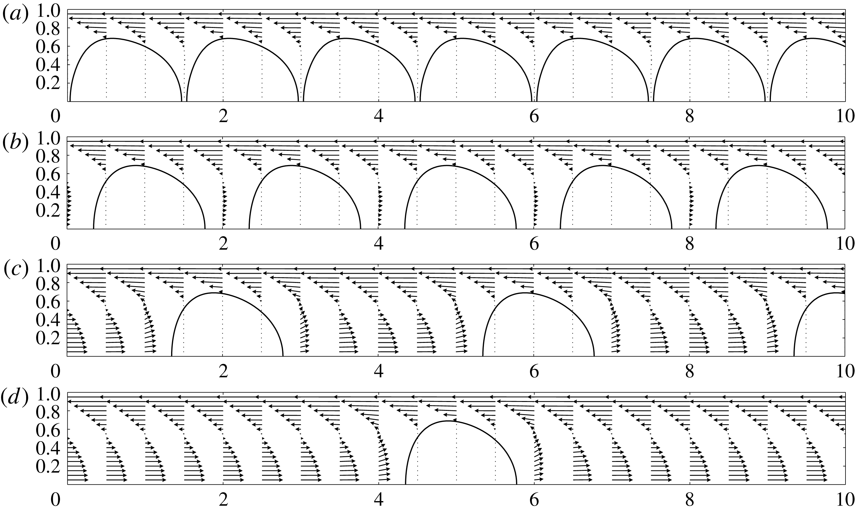
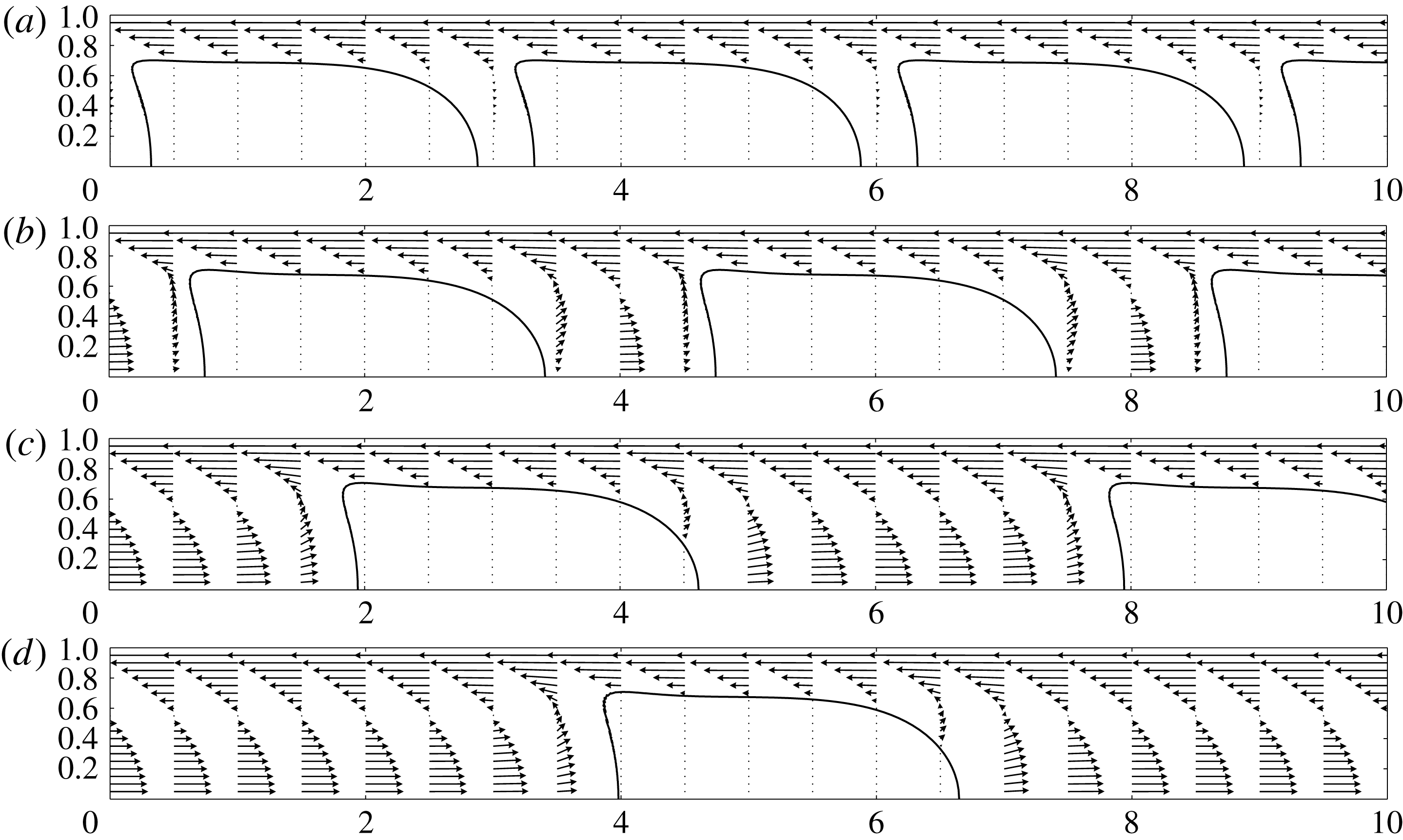
Representative flow fields are depicted in figure 5 for trains of ‘sphere-like’ vesicles under moderate confinement and various inter-vesicle spacings (
 $\unicode[STIX]{x1D710}=0.99$
,
 $\unicode[STIX]{x1D706}=0.7$
,
 $\unicode[STIX]{x1D706}/\unicode[STIX]{x1D706}_{c}=0.64$
,
 $\unicode[STIX]{x1D6FF}=1.5{-}10$
). Flow fields for more elongated vesicles at roughly the same confinement (
 $\unicode[STIX]{x1D710}=0.8$
,
 $\unicode[STIX]{x1D706}=1$
,
 $\unicode[STIX]{x1D706}/\unicode[STIX]{x1D706}_{c}=0.61$
,
 $\unicode[STIX]{x1D6FF}=3{-}10$
) are shown in figure 6. In these simulations,
 $\unicode[STIX]{x1D6FD}=0$
and
 $\unicode[STIX]{x1D705}=1$
. The velocity vectors are drawn in a reference frame moving with the vesicle train at steady velocity
 $U$
. As indicated previously, the interior fluid velocity is stagnant in the moving reference frame. Thus, the vesicle train resembles a line of rigid particles. The flow in the gap separating the vesicle membrane and the tube wall is a simple shear flow with a velocity gradient equal to the train velocity
 $U$
divided by the gap thickness. As the separation parameter
 $\unicode[STIX]{x1D6FF}$
decreases to the point at which neighbouring vesicles are closely spaced, the interstitial fluid between vesicles moves with the train velocity
 $U$
.
Velocity field from 3D BEM simulations. Results are shown for
 $\unicode[STIX]{x1D710}=0.99$
,
 $\unicode[STIX]{x1D706}=0.7$
,
 $\unicode[STIX]{x1D6FD}=0$
,
 $\unicode[STIX]{x1D705}=1$
: (a)
 $\unicode[STIX]{x1D6FF}=1.5$
, (b)
 $\unicode[STIX]{x1D6FF}=2$
, (c)
 $\unicode[STIX]{x1D6FF}=4$
and (d)
 $\unicode[STIX]{x1D6FF}=10$
.

Velocity field from 3D BEM simulations. Results are shown for
 $\unicode[STIX]{x1D710}=0.80$
,
 $\unicode[STIX]{x1D706}=1$
,
 $\unicode[STIX]{x1D6FD}=0$
,
 $\unicode[STIX]{x1D705}=1$
: (a)
 $\unicode[STIX]{x1D6FF}=3$
, (b)
 $\unicode[STIX]{x1D6FF}=4$
, (c)
 $\unicode[STIX]{x1D6FF}=6$
and (d)
 $\unicode[STIX]{x1D6FF}=10$
.

Previous studies of periodic trains of rigid particles in bounded Poiseuille flow have shown that the relative velocity
 $U/V$
is relatively insensitive to the value of the separation parameter
 $\unicode[STIX]{x1D6FF}$
(Wang & Skalak Reference Wang and Skalak1969; Chen & Skalak Reference Chen and Skalak1970). The present simulations verify this trend: vesicle trains in which the vesicles are either nearly touching (
 $\unicode[STIX]{x1D6FF}R\simeq L$
, where
 $L$
is the vesicle length) or well separated (
 $\unicode[STIX]{x1D6FF}R\gg L$
) exhibit as large as a 2 % difference in
 $U/V$
. The corresponding change to the dimensionless pressure drop
 $\unicode[STIX]{x0394}p^{+}R/(\unicode[STIX]{x1D707}V)$
is
 $O(1)$
, which is negligible compared to the relative change with confinement. The insensitivity of these parameters to changes in
 $\unicode[STIX]{x1D6FF}$
is attributable to the exponentially decaying velocity disturbance in conduit flow. Since the effect of
 $\unicode[STIX]{x1D6FF}$
on trains of rigid particles has already been studied extensively by other authors (Wang & Skalak Reference Wang and Skalak1969; Chen & Skalak Reference Chen and Skalak1970), it will not be discussed further in this work. The remainder of this paper is devoted to the parameter space that is unique to vesicles – namely, the interplay of confinement, reduced volume, and bending elasticity. Unless otherwise indicated, all simulations reported below are for
 $\unicode[STIX]{x1D6FF}=10$
(all vesicle lengths
 $L$
computed are smaller than
 $10R$
). In these cases, vesicle–vesicle interactions may be safely neglected and one need only consider a single vesicle.
5.2 Symmetry breaking and time-dependent states
In this section, some attention is given to the emergence of (rotationally) asymmetric and time-dependent states in the 3D BEM simulations. Such phenomena cannot be predicted using the lubrication approximation of § 4, as steadiness and axisymmetry are assumed a priori in that theory. These assumptions are justified by the fact that, when the ratio
 $\unicode[STIX]{x1D706}/\unicode[STIX]{x1D706}_{c}$
is sufficiently close to unity, cylindrical confinement suppresses the formation of asymmetric shape modes. However, when the reduced volume
 $\unicode[STIX]{x1D710}$
and radius ratio
 $\unicode[STIX]{x1D706}$
are small enough (criteria to be made more precise in due course), an initially axisymmetric vesicle may in fact break symmetry even though the imposed flow field is axisymmetric.
Before proceeding any further, it is instructive to review previously published studies of vesicle shape dynamics in Poiseuille flows. Danker et al. (Reference Danker, Vlahovska and Misbah2009) published the first small-deformation theory for vesicles in quadratic flow fields, focusing on the migration phenomenon when the vesicle is displaced from the flow centreline. In this situation, the flow field is dominated by the shear contribution and the quadratic part supplies only a weak correction. Farutin & Misbah (Reference Farutin and Misbah2011) later reported a phase diagram for vesicle shapes parametrized by the bending parameter
 $\unicode[STIX]{x1D6FD}$
(defined in their paper as the reciprocal of a ‘bending capillary number’), again using small-deformation theory. They reported only axisymmetric shapes when the vesicle is on the centreline and asymmetric shapes when off the centreline. The former results were later confirmed by experiments of Coupier et al. (Reference Coupier, Farutin, Minetti, Podgorski and Misbah2012). Later, Farutin & Misbah (Reference Farutin and Misbah2014) conducted 3D BEM simulations and reported symmetry-breaking vesicle shapes – including the so-called ‘croissant’ and ‘slipper’ shapes – at the centreline of unbounded, circular Poiseuille flow when the bending parameter
 $\unicode[STIX]{x1D6FD}$
is sufficiently large. As
 $\unicode[STIX]{x1D6FD}$
was decreased, the axisymmetric state was recovered in their simulations.
All of the aforementioned studies focused on vesicles of reduced volumes
 $\unicode[STIX]{x1D710}$
near unity. Kaoui et al. (Reference Kaoui, Tahiri, Biben, Ez-Zahraouy, Benyoussef, Biros and Misbah2011) and later Aouane et al. (Reference Aouane, Thiebaud, Benyoussef, Wagner and Misbah2014) employed the 2D boundary integral method to map out the vesicle shape configuration space for a wide range of the parameters
 $\unicode[STIX]{x1D710}$
,
 $\unicode[STIX]{x1D706}$
and
 $\unicode[STIX]{x1D6FD}$
in the 2D geometry. These authors uncovered a rich phase space containing a variety of vesicle shape morphologies. Among these, 2D asymmetric shapes were observed for concentrically positioned vesicles of low reduced volume, including the slipper shape. Kaoui et al. (Reference Kaoui, Tahiri, Biben, Ez-Zahraouy, Benyoussef, Biros and Misbah2011) also reported some preliminary 3D calculations for planar Poiseuille flow, but provided only a sparse discussion of their results.
As pointed out by Kaoui et al. (Reference Kaoui, Tahiri, Biben, Ez-Zahraouy, Benyoussef, Biros and Misbah2011), determination of the phase diagram for 3D vesicle shape morphologies in circular Poiseuille flow remains a computationally intensive task. 3D computations take significantly longer to complete than the analogous 2D computations. Moreover, circular Poiseuille flow is a more intensive calculation than planar Poiseuille flow due to the enhanced vesicle–wall interactions. Compounding this increase in computational time are three issues. Firstly, the phase space for the nonlinear dynamical problem is vast, spanning all possible values of
 $\unicode[STIX]{x1D710}$
,
 $\unicode[STIX]{x1D706}$
and
 $\unicode[STIX]{x1D6FD}$
(in addition to
 $\unicode[STIX]{x1D705}$
and
 $\unicode[STIX]{x1D6FF}$
). Secondly, the nonlinear shape evolution may be slow, requiring a prohibitively long time to reach steady state. Lastly, it is not clear a priori whether a steady state exists or if the vesicle shape will become unstable. This latter concern is supported by the vast literature documenting the onset of shape instabilities in the presence of a straining field (Kantsler et al.
Reference Kantsler, Segre and Steinberg2008a
; Zhao & Shaqfeh Reference Zhao and Shaqfeh2013b
; Narsimhan et al.
Reference Narsimhan, Spann and Shaqfeh2014, Reference Narsimhan, Spann and Shaqfeh2015).
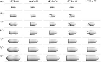
Time sequence of the vesicle shape evolved from an initially equilibrium configuration. Results were computed via 3D BEM for
 $\unicode[STIX]{x1D710}=0.8$
,
 $\unicode[STIX]{x1D705}=1$
,
 $\unicode[STIX]{x1D6FD}=0.02$
,
 $\unicode[STIX]{x1D6FF}=10$
, with values of
 $\unicode[STIX]{x1D706}$
: (a) 0.4, (b) 0.6, (c) 0.7, (d) 0.8, (e) 0.9, (f) 1 and (g) 1.2. At this reduced volume,
 $\unicode[STIX]{x1D706}_{c}=1.64$
. Vesicles for which
 $\unicode[STIX]{x1D706}<0.9$
transition to an asymmetric secondary shape at longer times.

As it is not the objective of this paper to map out the entire phase diagram for the 3D geometry, only some of the salient features of the shape dynamics in 3D are presented here. These include long-time shape transitions from axisymmetric to asymmetric states when
 $\unicode[STIX]{x1D710}\lesssim 0.85$
. A representative example is shown in figure 7 for
 $\unicode[STIX]{x1D710}=0.8$
,
 $\unicode[STIX]{x1D6FD}=0.02$
, and various values of
 $\unicode[STIX]{x1D706}$
. At this reduced volume, the vesicle remains in a steady, axisymmetric configuration (up to
 $tV/R=100$
) for
 $\unicode[STIX]{x1D706}>0.9$
(the so-called ‘parachute’ shape, shown in figure 7
e–g). However, once less confined the vesicle spontaneously breaks symmetry at later times, resulting in an asymmetric shape with two rear lobes that align along the local rate of extension (figure 7
b–d). The time at which this shape transition occurs depends on the degree of confinement. As can be seen from comparing figures 7(b), 7(c), and 7(d), increasing
 $\unicode[STIX]{x1D706}$
delays the onset of the transition. The existence of two ‘long-lived’ states for this particular parameter set lends evidence for multiple fixed points of the (nonlinear) evolution equation for the surface position
 $\boldsymbol{x}_{s}(\boldsymbol{x},t)$
(cf. (2.9)–(2.12)). Smaller vesicles (i.e., lower values of
 $\unicode[STIX]{x1D706}$
) exhibit different shape morphologies, including the slipper shape shown in figure 7(a). Similar observations were reported by Aouane et al. (Reference Aouane, Thiebaud, Benyoussef, Wagner and Misbah2014) in 2D.
It is not clear whether or not the latter-stage states shown in figure 7 for
 $\unicode[STIX]{x1D706}<0.9$
are steady. Literature precedent suggests that the rear lobes shown in figure 7(b–d) will feel a local extensional field and therefore should elongate over time. Membrane curvature gradients drive this elongation (akin to the Rayleigh–Plateau instability), whereas finite bending resistance will confer a stabilizing effect (Narsimhan et al.
Reference Narsimhan, Spann and Shaqfeh2014). As the local extensional field is relatively weak, the evolution of the secondary shape is slow (note, for instance, the small difference between time points
 $tV/R=54$
and 72 in figure 7
c). The evolution of the slipper shape shown in figure 7(a) is similarly slow (i.e., noticeable shape change occurs over 10–100
 $tV/R$
). In their 2D calculations, Aouane et al. (Reference Aouane, Thiebaud, Benyoussef, Wagner and Misbah2014) reported that the slipper shape moves like a spermatozoon and exhibits period-doubling dynamics. It is expected that the simulations reported in figure 7 would have to be continued for hundreds of dimensionless time points
 $tV/R$
in order to ascertain whether the system is steady or unstable (equivalent to weeks or months of computer time on a massively parallel supercomputer). In view of these possibilities, the term ‘long-lived state’ is preferred over ‘steady state’ to describe the latter-stage vesicle shapes in figure 7(a–d).
Time-dependent states and symmetry breaking are also observed at lower reduced volumes. For
 $\unicode[STIX]{x1D710}=0.7$
and
 $\unicode[STIX]{x1D6FD}=0.02$
, a slight asymmetry in the membrane velocity profile induces tank treading in the direction perpendicular to the flow axis when
 $\unicode[STIX]{x1D706}\lesssim 1.2$
. This in turn creates an ‘asymmetric parachute’ shape akin to those predicted by Zhao et al. (Reference Zhao, Isfahani, Olson and Freund2010) for red blood cells. The two-lobed shape is also observed at lower reduced volume, with the transition occurring around
 $\unicode[STIX]{x1D706}\simeq 1.1$
for
 $\unicode[STIX]{x1D710}=0.7$
(as compared to
 $\unicode[STIX]{x1D706}\simeq 0.8$
for
 $\unicode[STIX]{x1D710}=0.8$
, shown in figure 7
d). Further discussion of these cases, as well as an exhaustive parametric study of the dynamics of vesicles in 3D bounded Poiseuille flows, is beyond the scope of the present work.
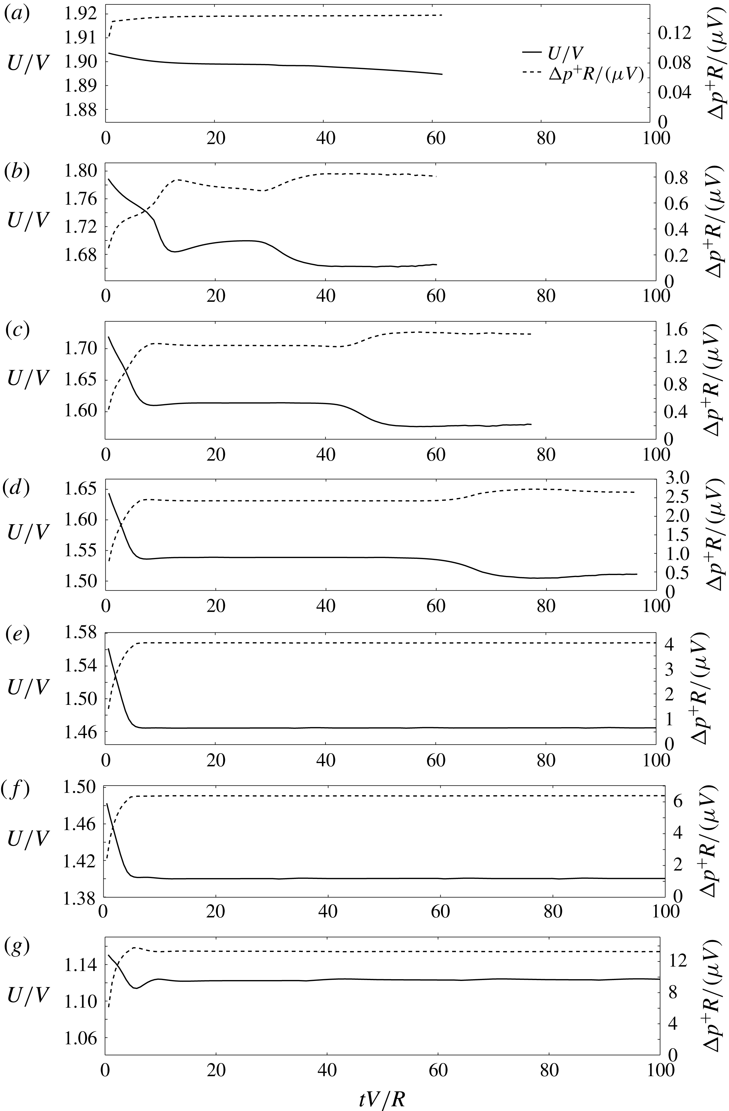
Time series of the relative velocity
 $U/V$
and dimensionless extra pressure drop
 $\unicode[STIX]{x0394}p^{+}R/(\unicode[STIX]{x1D707}V)$
for the 3D BEM simulations shown in figure 7.

In order to gauge how the shape transitions reported in figure 7 affect the Stokes disturbance field, the relative velocity
 $U/V$
and dimensionless extra pressure drop
 $\unicode[STIX]{x0394}p^{+}R/(\unicode[STIX]{x1D707}V)$
are plotted over time in figure 8. The time-dependent shape transitions induce a 2 %–3 % relative change in
 $U/V$
and up to a 70 % relative change in
 $\unicode[STIX]{x0394}p^{+}R/(\unicode[STIX]{x1D707}V)$
. However, it is worth emphasizing that these deviations are small compared to those incurred by increasing vesicle confinement. This is easily deduced by examining the scale of the ordinate in figure 8(a–g). The relative velocity
 $U/V$
decreases in proportion to
 $\unicode[STIX]{x1D706}$
at an
 $O(1)$
rate, while the dimensionless extra pressure drop
 $\unicode[STIX]{x0394}p^{+}R/(\unicode[STIX]{x1D707}V)$
increases precipitously (i.e., exponentially) with increasing
 $\unicode[STIX]{x1D706}$
.
From these observations, one may arrive at a rather intuitive conclusion: the detailed vesicle shape is less significant than its size in determining hydrodynamical figures of merit. Deviations in vesicle shape morphology induced by unsteadiness contribute relatively small corrections to
 $U/V$
and
 $\unicode[STIX]{x0394}p^{+}R/(\unicode[STIX]{x1D707}V)$
once the influence of the other dimensionless parameters are taken into account. Among these, the geometric parameters (
 $\unicode[STIX]{x1D710}$
and
 $\unicode[STIX]{x1D706}$
) are expected to have the greatest impact. A comprehensive discussion of the effects of these parameters is presented in the next section. The influence of the bending parameter
 $\unicode[STIX]{x1D6FD}$
is later examined in § 5.4.
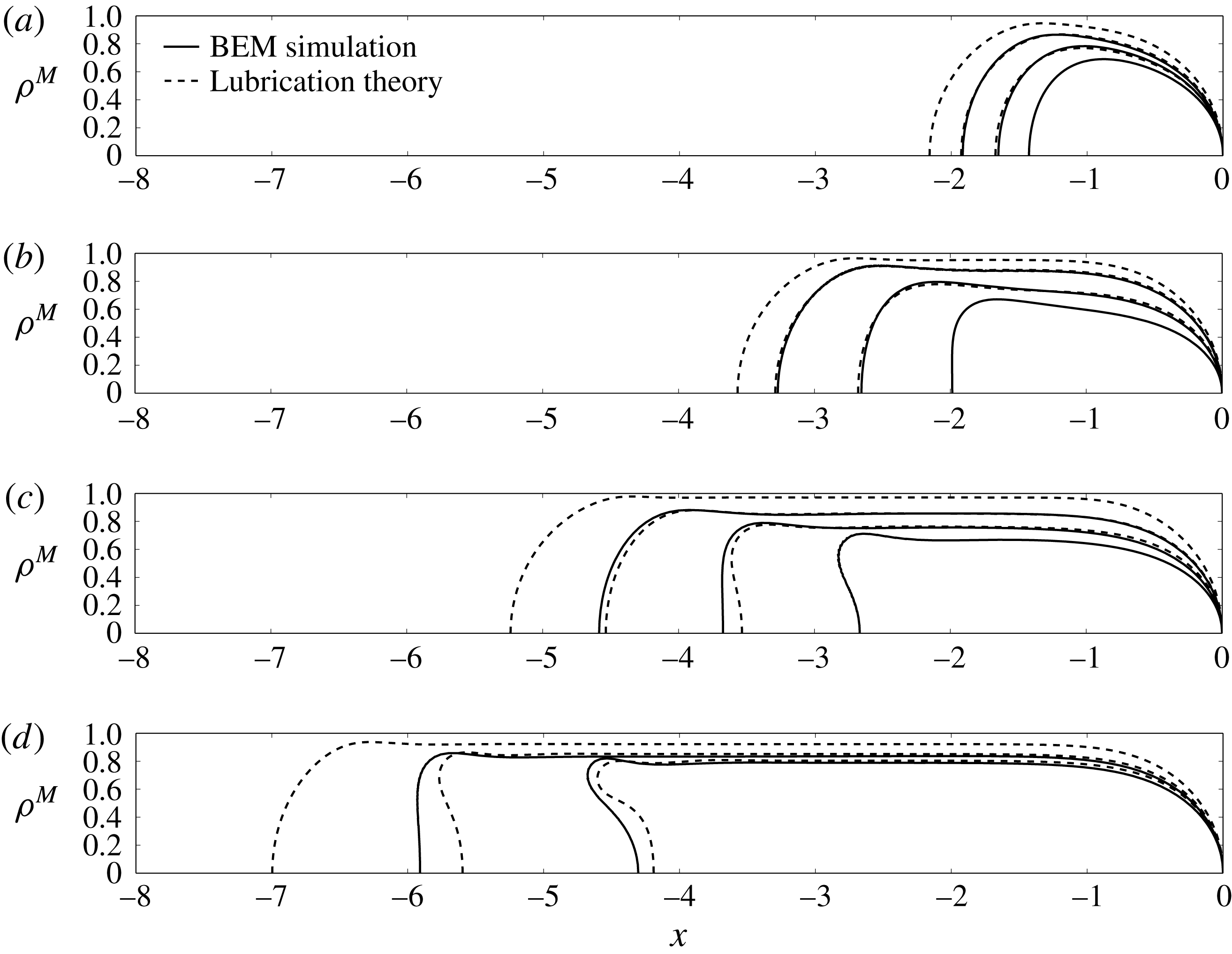
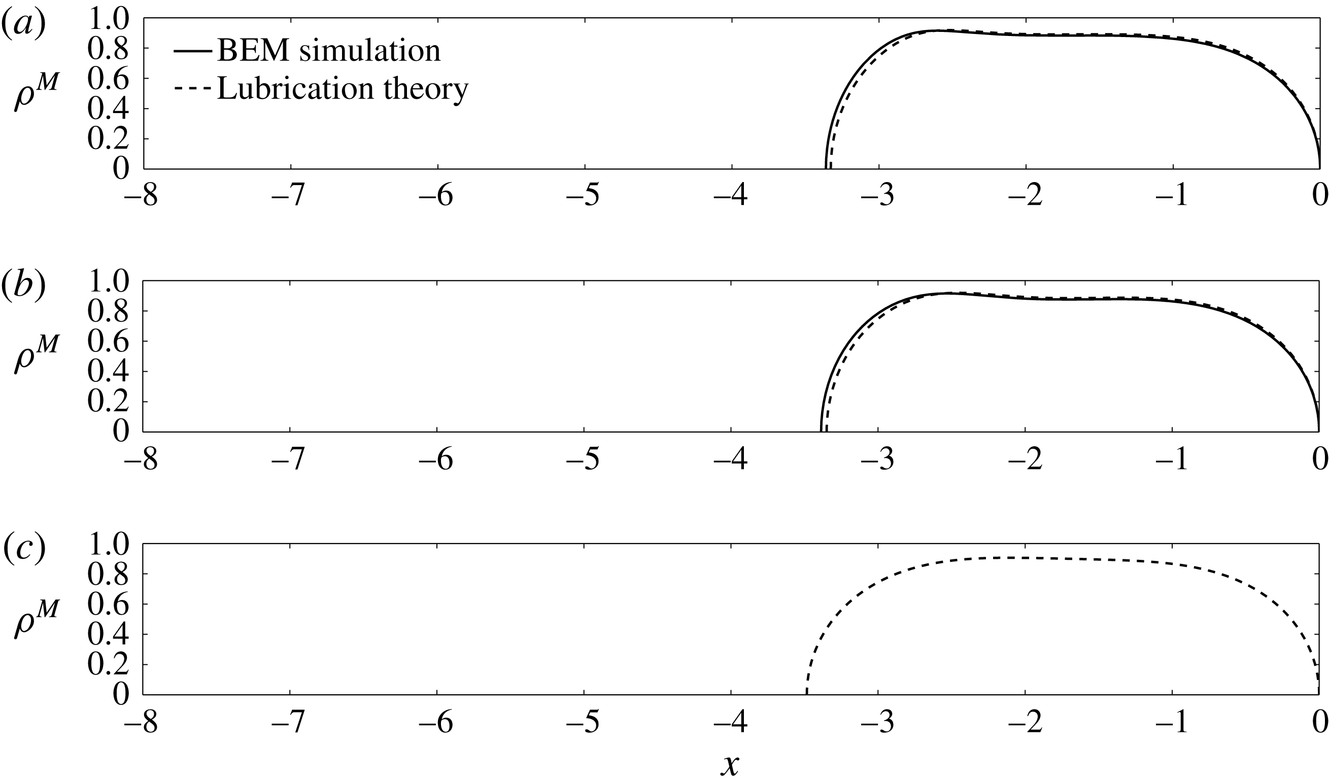
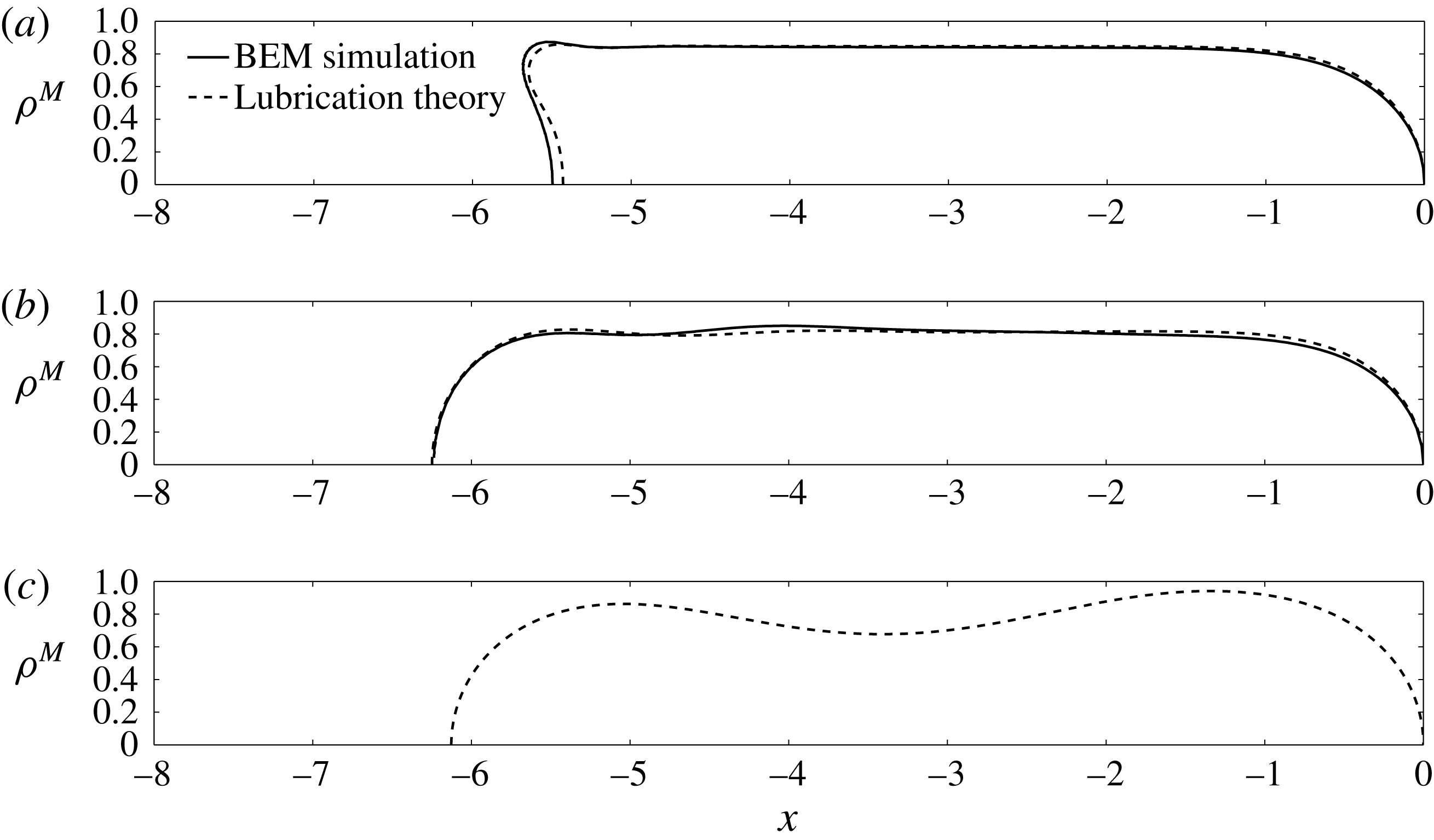
Vesicle shapes computed by 3D BEM simulation (solid lines) and axisymmetric lubrication theory (dashed lines) for
 $\unicode[STIX]{x1D705}=1$
,
 $\unicode[STIX]{x1D6FD}=0.02$
, and
 $\unicode[STIX]{x1D6FF}=10$
. (a)
 $\unicode[STIX]{x1D710}=0.99$
, BEM:
 $\unicode[STIX]{x1D706}=0.9$
, 0.8, 0.7; LT:
 $\unicode[STIX]{x1D706}=1$
, 0.9, 0.8. (b)
 $\unicode[STIX]{x1D710}=0.9$
, BEM:
 $\unicode[STIX]{x1D706}=1.2$
, 1, 0.8; LT:
 $\unicode[STIX]{x1D706}=1.3$
, 1.2, 1. (c)
 $\unicode[STIX]{x1D710}=0.8$
, BEM:
 $\unicode[STIX]{x1D706}=1.4$
, 1.2, 1; LT:
 $\unicode[STIX]{x1D706}=1.6$
, 1.4, 1.2. (d)
 $\unicode[STIX]{x1D710}=0.7$
, BEM:
 $\unicode[STIX]{x1D706}=1.6$
, 1.4; LT:
 $\unicode[STIX]{x1D706}=1.8$
, 1.6, 1.4.

5.3 Effect of confinement and reduced volume
Figure 9 shows steady, axisymmetric vesicle shapes in bounded tube flow as computed via 3D BEM simulation and axisymmetric lubrication theory. For the range of reduced volumes
 $\unicode[STIX]{x1D710}$
and radius ratios
 $\unicode[STIX]{x1D706}$
shown, no indications of unsteady behaviour are observed within the time frame of the simulation (up to
 $tV/R=100$
). The bending parameter is set to a small value
 $\unicode[STIX]{x1D6FD}=0.02$
to minimize the effect of bending elasticity while also avoiding numerical instabilities associated with high-wavenumber shape fluctuations. Reduced volumes near unity are ‘sphere-like’ and deform very little due to flow. As the reduced volume decreases at fixed confinement
 $\unicode[STIX]{x1D706}/\unicode[STIX]{x1D706}_{c}$
, the vesicle elongates and the rear tail of the vesicle can develop concave curvature. The lubrication theory does a remarkable job of reproducing the vesicle shape from the fully 3D BEM simulations. The error in the calculated shape increases as the reduced volume is decreased, with the maximum local error at the rear tail (as large as 5 % for
 $\unicode[STIX]{x1D710}=0.7$
). There are two sources of error that can explain the discrepancy. The first is the relative change in surface area during shape evolution in the BEM simulations, which can result in global changes to the vesicle shape for a target surface area
 $A_{0}$
. Second, the Stokes velocity field at the rear end of the vesicle is approximated by a quasi-parallel flow in the lubrication approximation, which is not strictly valid. As shown in figures 5 and 6, the flow near the front and rear ends is not exactly unidirectional. Non-parallel velocity components contribute additional normal and shear tractions (neglected in (4.7)–(4.8)), which in turn affect the membrane tension
 $\unicode[STIX]{x1D70F}$
, pressure
 $p$
, and vesicle shape. The error in neglecting these membrane tractions become increasingly significant as the rear tail develops concave curvature (typically, this occurs when
 $\unicode[STIX]{x1D710}\lesssim 0.85$
and
 $\unicode[STIX]{x1D706}/\unicode[STIX]{x1D706}_{c}\lesssim 0.85$
).
Relative velocity
 $U/V$
plotted against the radius ratio
 $\unicode[STIX]{x1D706}$
for a range of reduced volumes
 $\unicode[STIX]{x1D710}$
(
 $\unicode[STIX]{x1D705}=1$
,
 $\unicode[STIX]{x1D6FD}=0.02$
,
 $\unicode[STIX]{x1D6FF}=10$
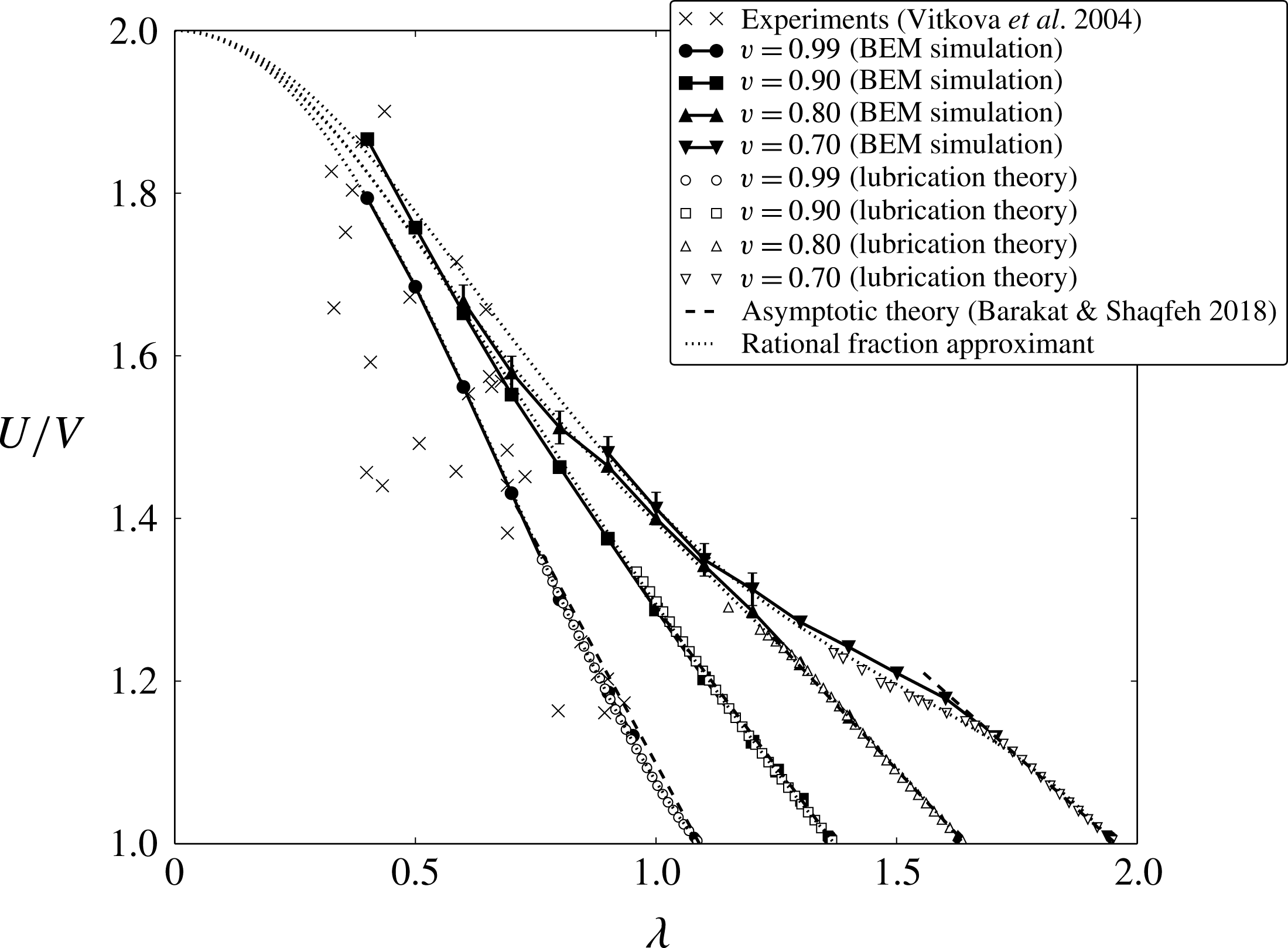
). Shown are the experimental measurements of Vitkova et al. (Reference Vitkova, Mader and Podgorski2004), calculations via 3D BEM simulation and axisymmetric lubrication theory, the correlation (1.2a
) of Barakat & Shaqfeh (Reference Barakat and Shaqfeh2018) (dashed curves), and the rational fraction approximant (5.2a
) (dotted curves). Where appropriate, error bars are used to quantify the maximum change observed after start-up in the BEM simulations.

The relative velocity
 $U/V$
is plotted against
 $\unicode[STIX]{x1D706}$
for several values of
 $\unicode[STIX]{x1D710}$
in figure 10. In addition to the simulations that reached steady state, unsteady results are plotted if the vesicle attains a ‘long-lived state’ (i.e., marginal shape change occurs over
 ${\sim}50~tV/R$
). In these latter cases, error bars are used to indicate the maximum change in the relative velocity over time after the initial start-up period. The bending parameter is again kept small (
 $\unicode[STIX]{x1D6FD}=0.02$
) so that bending elasticity has a negligible effect on the Stokes flow. The experimental measurements of Vitkova et al. (Reference Vitkova, Mader and Podgorski2004) are plotted for comparison and show excellent agreement with the simulation results for
 $\unicode[STIX]{x1D710}=0.9{-}0.99$
. Near
 $\unicode[STIX]{x1D706}=\unicode[STIX]{x1D706}_{c}$
, the enormous number of mesh elements required in order to resolve the lubrication interaction renders the BEM simulation computationally infeasible. Fortunately, the axisymmetric lubrication theory nicely interpolates the simulation data with the asymptotic correlation (1.2a
) of Barakat & Shaqfeh (Reference Barakat and Shaqfeh2018). Of particular note is the data for
 $\unicode[STIX]{x1D710}=0.70$
, wherein the lubrication theory accurately captures the transition from a ‘spherocylinder’ shape to a ‘parachute’ shape around
 $\unicode[STIX]{x1D706}=1.7$
(also shown in figure 9
d). This transition is accompanied by a sharp decrease in vesicle length and a comparably smaller change in the separation gap distance, which in turn decreases the rate of change of
 $U/V$
with respect to
 $\unicode[STIX]{x1D706}$
. The theory of Barakat & Shaqfeh (Reference Barakat and Shaqfeh2018), which assumes weak perturbations from the spherocylinder shape, cannot capture this shape transition.
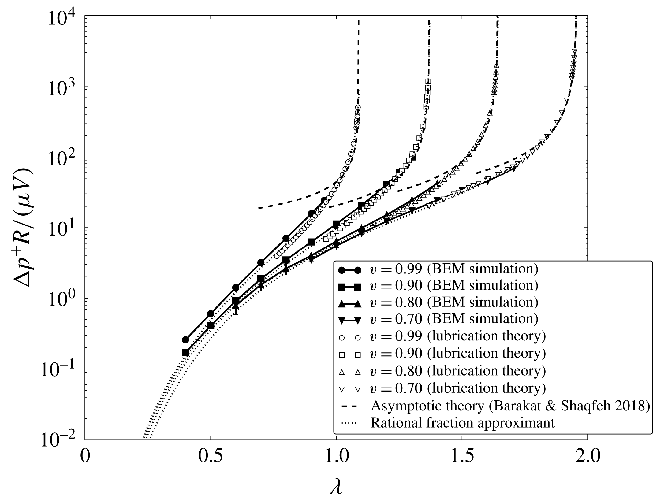
The dimensionless extra pressure drop
 $\unicode[STIX]{x0394}p^{+}R/(\unicode[STIX]{x1D707}V)$
is plotted against
 $\unicode[STIX]{x1D706}$
in figure 11 for the same set of conditions reported in figure 10. Again, error bars are used to quantify the maximum deviation after start-up when long-lived unsteadiness is observed in the BEM simulations. Unfortunately, no experimental results are available for this flow geometry. Again, the lubrication theory nicely interpolates the BEM simulation data with the asymptotic prediction (1.2b
) of Barakat & Shaqfeh (Reference Barakat and Shaqfeh2018). This is a crucial improvement, because the drag is singular in the limit as
 $\unicode[STIX]{x1D706}\rightarrow \unicode[STIX]{x1D706}_{c}$
. Consequently, the perturbative approximation (1.2b
) with respect to the small parameter
 $(1-\unicode[STIX]{x1D706}/\unicode[STIX]{x1D706}_{c})$
overestimates
 $\unicode[STIX]{x0394}p^{+}R/(\unicode[STIX]{x1D707}V)$
when
 $\unicode[STIX]{x1D706}$
is not close to
 $\unicode[STIX]{x1D706}_{c}$
. The present lubrication theory, which makes no assumptions about the smallness of
 $(1-\unicode[STIX]{x1D706}/\unicode[STIX]{x1D706}_{c})$
, introduces a negative correction.
Dimensionless extra pressure drop
 $\unicode[STIX]{x0394}p^{+}R/(\unicode[STIX]{x1D707}V)$
plotted against the radius ratio
 $\unicode[STIX]{x1D706}$
for a range of reduced volumes
 $\unicode[STIX]{x1D710}$
(
 $\unicode[STIX]{x1D705}=1$
,
 $\unicode[STIX]{x1D6FD}=0.02$
,
 $\unicode[STIX]{x1D6FF}=10$
). Shown are calculations from 3D BEM simulations, the axisymmetric lubrication theory, the correlation (1.2b
) of Barakat & Shaqfeh (Reference Barakat and Shaqfeh2018) (dashed curves), and the rational fraction approximant (5.2b
) (dotted curves). Where appropriate, error bars are used to quantify the maximum change observed after start-up in the BEM simulations.

Despite the wealth of numerical data presented in figures 10 and 11, it is desirable to unify these results by means of interpolation formulae. ‘Admissible’ interpolants are those which (i) follow the asymptotic prediction of Barakat & Shaqfeh (Reference Barakat and Shaqfeh2018) as
 $\unicode[STIX]{x1D706}/\unicode[STIX]{x1D706}_{c}\rightarrow 1$
; (ii) interpolate the numerical results from the 3D BEM simulations and axisymmetric lubrication theory; and (iii) exhibit the correct asymptotic behaviour as
 $\unicode[STIX]{x1D706}\rightarrow 0$
. The latter asymptote represents the physical situation of a freely suspended vesicle in a tube wherein the vesicle radius is small compared to the tube radius. Danker et al. (Reference Danker, Vlahovska and Misbah2009) studied this regime by means of small-deformation theory, but did not compute corrections to the relative velocity
 $U/V$
or dimensionless extra pressure drop
 $\unicode[STIX]{x0394}p^{+}R/(\unicode[STIX]{x1D707}V)$
as a result of deformation. As these corrections are expected to be relatively weak, as a first approximation one may replace the vesicle with a rigid sphere of the same diameter. Asymptotic approximations (in the limit
 $\unicode[STIX]{x1D706}\rightarrow 0$
) for rigid spheres in circular tubes are canonical (Wakiya Reference Wakiya1957; Brenner & Happel Reference Brenner and Happel1958; Brenner Reference Brenner1970); the most relevant results are
 $$\begin{eqnarray}\displaystyle & \displaystyle \frac{U}{V}=2-\frac{4}{3}(\unicode[STIX]{x1D710}^{1/3}\unicode[STIX]{x1D706})^{2}+O[(\unicode[STIX]{x1D710}^{1/3}\unicode[STIX]{x1D706})^{3}], & \displaystyle\end{eqnarray}$$
 $$\begin{eqnarray}\displaystyle & \displaystyle \frac{\unicode[STIX]{x0394}p^{+}R}{\unicode[STIX]{x1D707}V}=16(\unicode[STIX]{x1D710}^{1/3}\unicode[STIX]{x1D706})^{5}+O[(\unicode[STIX]{x1D710}^{1/3}\unicode[STIX]{x1D706})^{10}]. & \displaystyle\end{eqnarray}$$
 $\unicode[STIX]{x1D710}=1$
for spheres.) In (5.1), the small parameter
 $\unicode[STIX]{x1D706}$
has been ‘stretched’ by
 $\unicode[STIX]{x1D710}^{1/3}$
so that the dimensionless group
 $\unicode[STIX]{x1D710}^{1/3}\unicode[STIX]{x1D706}$
represents the ratio of the vesicle’s volumetric radius to the tube radius. The volumetric radius is defined here as the radius of a sphere with the same volume as the vesicle.
Taking (5.1) as the leading-order approximation for small
 $\unicode[STIX]{x1D706}$
, one may then utilize the BEM simulations, lubrication theory and asymptotic formulae (1.2) in order to construct approximate correlations for the whole range of
 $\unicode[STIX]{x1D706}$
. There are many ways in which one may construct such correlations – e.g., rational fraction (Padé) approximants are quite popular (Frost & Harper Reference Frost and Harper1976). The data shown in figures 10 and 11 are nicely interpolated by rational fractions of the form
 $$\begin{eqnarray}\displaystyle & \displaystyle \frac{U}{V}=2-\frac{4}{3}(\unicode[STIX]{x1D710}^{1/3}\unicode[STIX]{x1D706})^{2}\left[\frac{1+b_{1}\unicode[STIX]{x1D706}^{2}+b_{2}\unicode[STIX]{x1D706}^{4}+\cdots }{1+a_{1}\unicode[STIX]{x1D706}^{2}+a_{2}\unicode[STIX]{x1D706}^{4}+\cdots }\right], & \displaystyle\end{eqnarray}$$
 $$\begin{eqnarray}\displaystyle & \displaystyle \frac{\unicode[STIX]{x0394}p^{+}R}{\unicode[STIX]{x1D707}V}=16(\unicode[STIX]{x1D710}^{1/3}\unicode[STIX]{x1D706})^{5}\left[\frac{1+d_{1}\unicode[STIX]{x1D706}^{5}+d_{2}\unicode[STIX]{x1D706}^{6}+\cdots }{1+c_{1}\unicode[STIX]{x1D706}^{5}+c_{2}\unicode[STIX]{x1D706}^{6}+\cdots }\right], & \displaystyle\end{eqnarray}$$
 $a_{n}$
,
 $b_{n}$
,
 $c_{n}$
and
 $d_{n}$
are chosen to give the best fit to the data using nonlinear least-squares regression. These correlations are plotted as dotted curves in figures 10 and 11 using the parameters shown in table 1. The agreement with the numerical data is surprisingly good. It should be emphasized that the extrapolated predictions for small values of
 $\unicode[STIX]{x1D706}$
are only approximate; more detailed information about the lower asymptote is required to improve the predictions in this range.
Parameters
 $a_{n}$
,
 $b_{n}$
,
 $c_{n}$
and
 $d_{n}$
used in the rational fraction approximants (5.2) (plotted as dotted curves in figures 10 and 11), as determined by nonlinear least-squares regression. Also tabulated are the critical radius ratios
 $\unicode[STIX]{x1D706}_{c}$
for each reduced volume.

5.4 Effect of membrane bending elasticity
Barakat & Shaqfeh (Reference Barakat and Shaqfeh2018) noted that membrane bending elasticity – measured by the bending parameter
 $\unicode[STIX]{x1D6FD}$
– plays a minor role in disturbing the Stokes flow when
 $\unicode[STIX]{x1D706}/\unicode[STIX]{x1D706}_{c}$
is close to unity. The reason for this relative insensitivity to
 $\unicode[STIX]{x1D6FD}$
is that the available shape configuration space is restricted when the vesicle is near critical confinement. As
 $\unicode[STIX]{x1D706}$
decreases, it is expected that changing
 $\unicode[STIX]{x1D6FD}$
will have a more pronounced effect on the disturbance field produced by the vesicle, which in turn will affect the relative velocity and dimensionless extra pressure drop.
The numerical challenges associated with computing the membrane bending stresses in (2.9) are well documented (Guckenberger et al.
Reference Guckenberger, Schraml, Chen, Leonetti and Gekle2016). These challenges originate from the need to numerically compute high-order derivatives of the surface position
 $\boldsymbol{x}_{s}(\boldsymbol{x},t)$
in 3D. The scheme used in the present 3D BEM implementation relies on discretely evaluating the first variation of the Helfrich energy functional (2.8) using a smooth surrogate surface constructed by Loop subdivision (Loop Reference Loop1987; Zhao et al.
Reference Zhao, Spann and Shaqfeh2011), with an error that scales linearly with mesh size (Zhao & Shaqfeh Reference Zhao and Shaqfeh2013a
). It is possible to obtain accurate numerical simulations for
 $\unicode[STIX]{x1D6FD}=O(1)$
using this implementation. However, for large values of
 $\unicode[STIX]{x1D6FD}$
(the ‘weak-flow regime’), the numerical fidelity of the method breaks down as the system becomes dominated by membrane bending stresses. Large values of
 $\unicode[STIX]{x1D6FD}$
are therefore not accessible via 3D BEM. However, this latter regime is easily accessed using the aforementioned axisymmetric lubrication theory because the Laplace–Beltrami operator for the surface only requires computation of one-dimensional derivatives along the meridional contour. Since the full (axisymmetric) curvature operators are retained in (4.7), it is possible to resolve vesicle shapes very close to equilibrium. The limitation of this approach is that the accessible shape configuration space is now restricted to axisymmetric geometries. However, as shown previously, it is expected that the vesicle shape retains symmetry when it is highly confined. As this regime is of practical interest, the subsequent discussion will focus on confinement ratios
 $\unicode[STIX]{x1D706}/\unicode[STIX]{x1D706}_{c}$
near unity.
Vesicle shapes computed by 3D BEM simulation (solid lines) and axisymmetric lubrication theory (dashed lines) for
 $\unicode[STIX]{x1D710}=0.90$
,
 $\unicode[STIX]{x1D706}=1.22$
,
 $\unicode[STIX]{x1D705}=1$
, and
 $\unicode[STIX]{x1D6FF}=10$
(
 $\unicode[STIX]{x1D706}/\unicode[STIX]{x1D706}_{c}=0.89$
). (a)
 $\unicode[STIX]{x1D6FD}=0.02$
. (b)
 $\unicode[STIX]{x1D6FD}=2$
. (c)
 $\unicode[STIX]{x1D6FD}=200$
.

Vesicle shapes computed by 3D BEM simulation (solid lines) and axisymmetric lubrication theory (dashed lines) for
 $\unicode[STIX]{x1D710}=0.70$
,
 $\unicode[STIX]{x1D706}=1.58$
,
 $\unicode[STIX]{x1D705}=1$
, and
 $\unicode[STIX]{x1D6FF}=10$
(
 $\unicode[STIX]{x1D706}/\unicode[STIX]{x1D706}_{c}=0.81$
). (a)
 $\unicode[STIX]{x1D6FD}=0.02$
. (b)
 $\unicode[STIX]{x1D6FD}=2$
. (c)
 $\unicode[STIX]{x1D6FD}=200$
.

Figures 12 and 13 show the effect of membrane bending elasticity on the vesicle shape for two different reduced volumes (
 $\unicode[STIX]{x1D710}=0.90$
and 0.70) at high confinement. As the bending parameter
 $\unicode[STIX]{x1D6FD}$
increases, the vesicle is forced towards its ‘equilibrium’ configuration, which is both axisymmetric and mirror-plane symmetric. A full catalogue of equilibrium vesicle shapes has been documented by many authors, most notably by Seifert, Berndl & Lipowsky (Reference Seifert, Berndl and Lipowsky1991). As was previously shown in § 5.3, the accessible shape configuration space expands as the reduced volume
 $\unicode[STIX]{x1D710}$
is decreased. Consequently, the shape change with increasing
 $\unicode[STIX]{x1D6FD}$
illustrated in figure 13 is far more dramatic than in figure 12. Interestingly, the weak flow in figure 13(c) results in lobe swelling at the downstream end of the vesicle. This phenomenon is akin to the ‘slider block effect’, wherein a negative pressure created by flow into a wedge creates suction between two surfaces (Batchelor Reference Batchelor1967).
It is expected that the shape transformations described above have a marked effect on the disturbance field. In figure 14, the relative velocity
 $U/V$
and dimensionless extra pressure drop
 $\unicode[STIX]{x0394}p^{+}R/(\unicode[STIX]{x1D707}V)$
are plotted against the bending parameter
 $\unicode[STIX]{x1D6FD}$
for three different confinement ratios
 $\unicode[STIX]{x1D706}/\unicode[STIX]{x1D706}_{c}$
. All of the calculations presented in figure 14 are via axisymmetric lubrication theory, through which large data sets spanning many decades in
 $\unicode[STIX]{x1D6FD}$
can be obtained expeditiously. Clearly, the dependence of the hydrodynamic figures of merit on
 $\unicode[STIX]{x1D6FD}$
is highly complex, especially at low reduced volume. This complexity stems from the large family of shape configurations that the vesicle is able to access at low reduced volume. In the remainder of this section, special attention given to each of the cases shown in figure 14, with the aim of elucidating the competition between bending elasticity and viscous flow when vesicles are confined.
Relative velocity
 $U/V$
and dimensionless extra pressure drop
 $\unicode[STIX]{x0394}p^{+}R/(\unicode[STIX]{x1D707}V)$
plotted against the bending parameter
 $\unicode[STIX]{x1D6FD}$
for several values of
 $\unicode[STIX]{x1D710}$
and
 $\unicode[STIX]{x1D706}$
. All results shown were computed via axisymmetric lubrication theory. (a,d)
 $\unicode[STIX]{x1D706}/\unicode[STIX]{x1D706}_{c}=0.8$
. (b,e)
 $\unicode[STIX]{x1D706}/\unicode[STIX]{x1D706}_{c}=0.9$
. (c,f)
 $\unicode[STIX]{x1D706}/\unicode[STIX]{x1D706}_{c}=0.99$
.

At low to moderate confinement (figure 14
a–d), the vesicle shape undergoes a transition at some intermediate value of
 $\unicode[STIX]{x1D6FD}$
. The nature of this transition depends on the reduced volume
 $\unicode[STIX]{x1D710}$
. At high reduced volume (
 $\unicode[STIX]{x1D710}=0.99$
and 0.90), the transition is characterized by a modest enhancement of vesicle mobility (i.e., an increase in
 $U/V$
and decrease in
 $\unicode[STIX]{x0394}p^{+}R/(\unicode[STIX]{x1D707}V)$
). On examining figure 12, it becomes apparent that the vesicle shape near equilibrium (i.e., under weak flow) is more streamlined than the ‘pear’ shape that develops under stronger flow conditions. In the latter situation, the rear end of the vesicle occludes a greater portion of the tube cross-section, which in turn reduces its mobility.
At lower reduced volume (
 $\unicode[STIX]{x1D710}=0.80$
and 0.70), the transitions are much more complex due to the larger family of shapes that are accessible (as shown in figure 13). Still focusing for the time being on figure 14(a–d), it is apparent that increasing
 $\unicode[STIX]{x1D6FD}$
can result in either a reduction or an enhancement of vesicle mobility when
 $\unicode[STIX]{x1D710}$
is small. Typically, the ‘dumbbell’ shape characteristic of low-reduced-volume vesicles at equilibrium (
 $\unicode[STIX]{x1D6FD}\rightarrow \infty$
) is less streamlined than the ‘parachute’ shape that forms under strong flow conditions (
 $\unicode[STIX]{x1D6FD}\rightarrow 0$
). However, at some intermediate value of
 $\unicode[STIX]{x1D6FD}$
the vesicle can be forced into a shape that occludes nearly the entire tube cross-section, resulting in a local minimum value of
 $U/V$
and maximum value of
 $\unicode[STIX]{x0394}p^{+}R/(\unicode[STIX]{x1D707}V)$
. For a given reduced volume
 $\unicode[STIX]{x1D710}$
, the location of this extremum along the
 $\unicode[STIX]{x1D6FD}$
-axis is shifted to higher values with increasing confinement ratio
 $\unicode[STIX]{x1D706}/\unicode[STIX]{x1D706}_{c}$
.
At near-critical confinement (figure 14
e,f), the shape configuration space becomes highly restricted. Increasing
 $\unicode[STIX]{x1D6FD}$
in this regime forces the vesicle into a shape that is geometrically prohibited by the tube boundary, resulting in very narrow separation distances. That is to say, the ‘equilibrium shape’ that the vesicle would likely adopt in an unbounded, weak flow (as
 $\unicode[STIX]{x1D6FD}\rightarrow \infty$
) cannot be accessed. Thus, a local extremum with respect to
 $\unicode[STIX]{x1D6FD}$
is not observed for near-critical confinement. Rather, the vesicle mobility continues to drop with increasing
 $\unicode[STIX]{x1D6FD}$
, in accordance with predictions made by Barakat & Shaqfeh (Reference Barakat and Shaqfeh2018) (figure 8 of their paper).
6 Conclusions
The motion of vesicles in circular tubes has been studied using a combination of 3D BEM simulations and lubrication theory. The relative velocity
 $U/V$
and dimensionless extra pressure drop
 $\unicode[STIX]{x0394}p^{+}R/(\unicode[STIX]{x1D707}V)$
were computed as functions of reduced volume, confinement and membrane bending stiffness. It was shown that the reduced volume
 $\unicode[STIX]{x1D710}$
and radius ratio
 $\unicode[STIX]{x1D706}$
had the most pronounced impact on vesicle hydrodynamics. Decreasing
 $\unicode[STIX]{x1D710}$
tends to ‘streamline’ the vesicle body and hence increase
 $U/V$
. Increasing the vesicle size tends to enhance the wall friction force and hence
 $\unicode[STIX]{x0394}p^{+}R/(\unicode[STIX]{x1D707}V)$
. Rational fraction approximants for
 $U/V$
and
 $\unicode[STIX]{x0394}p^{+}R/(\unicode[STIX]{x1D707}V)$
were developed (cf. (5.2)) and extend a previous correlation given by Barakat & Shaqfeh (Reference Barakat and Shaqfeh2018), which is asymptotically valid in the limit as the confinement ratio
 $\unicode[STIX]{x1D706}/\unicode[STIX]{x1D706}_{c}\rightarrow 1$
. The latter correlation is appropriate when the vesicle shape is very nearly a spherocylinder.
At lower values of
 $\unicode[STIX]{x1D710}$
and
 $\unicode[STIX]{x1D706}$
, asymmetric vesicle shapes were observed. Some of these have no analogue in 2D and, to the best of the authors’ knowledge, have not been reported elsewhere. It was shown that asymmetric modes can be excited after the start-up period, with a time delay (ranging from
 $\unicode[STIX]{x0394}tV/R=1{-}10$
) that depends on the degree of confinement. Various shape morphologies were observed, including the ‘slipper’ shape and ‘two-lobed’ shape, and continue to evolve in time. Despite this unsteadiness, the relative changes to the vesicle velocity and extra pressure drop were small compared to geometrically induced changes (i.e., changing the confinement or reduced volume). Further study into vesicle symmetry breaking in quadratic flows remains an open and interesting area, though it is beyond the scope of the present work.
Changing the separation parameter
 $\unicode[STIX]{x1D6FF}$
had little effect on the morphology and hydrodynamics of the periodic train. By contrast, the bending parameter
 $\unicode[STIX]{x1D6FD}$
has a marked impact – by increasing
 $\unicode[STIX]{x1D6FD}$
, the vesicle tends to return to its ‘equilibrium shape’ and significantly alters the geometry. The effect of bending stiffness is highly nonlinear and qualitatively dependent on the other dimensionless groups, as the reduced volume
 $\unicode[STIX]{x1D710}$
and radius ratio
 $\unicode[STIX]{x1D706}$
effectively restricts the accessible shape configuration space. At high confinement (large
 $\unicode[STIX]{x1D706}$
), increasing
 $\unicode[STIX]{x1D6FD}$
tends to increase the dissipation in the thin fluid layer, thus enhancing the wall drag and decreasing vesicle mobility.
The results of this study can be used in capillary-flow experiments to correlate hydrodynamical figures of merit –
 $U/V$
and
 $\unicode[STIX]{x0394}p^{+}R/(\unicode[STIX]{x1D707}V)$
– to vesicle shape deformation. Specifically, the strong dependence of these quantities on the reduced volume
 $\unicode[STIX]{x1D710}$
and radius ratio
 $\unicode[STIX]{x1D706}$
suggests a means for accurately predicting
 $\unicode[STIX]{x1D710}$
and
 $\unicode[STIX]{x1D706}$
by simultaneously measuring
 $U/V$
and
 $\unicode[STIX]{x0394}p^{+}R/(\unicode[STIX]{x1D707}V)$
. Such measurements do not require advanced microscopy techniques and can be used in tandem with the results of this work – in particular, the correlations (5.2) – to extract important geometric information on a confined vesicle system. Uncertainties associated with shape asymmetries, unsteadiness, and membrane bending stiffness are also quantified in this work.
Acknowledgements
The authors acknowledge support from the National Science Foundation (CBET 1066263/1066334). J.M.B. was supported by a Graduate Research Fellowship from the National Science Foundation. J.M.B. would like to acknowledge several people: Dr A. Spann, for early development of the 3D BEM code; Dr J. Einarsson, for conversations that led to understanding vesicle hydrodynamics at low confinement; and Dr S. Vanapalli, for many fruitful discussions of practical microfluidic measurements.